From Data-Rich to Data-Scarce: Spatiotemporal Evaluation of a Hybrid Wavelet-Enhanced Deep Learning Model for Day-Ahead Wind Power Forecasting Across Greece

Abstract

Efficient wind power forecasting is critical in achieving large-scale integration of wind energy in modern electricity systems. On the other hand, limited availability of wealthy, long-term historical data of wind power generation for many sites of interest often challenges the training of tailored forecasting models, which, in turn, introduces uncertainty concerning the anticipated operational status of similar early-life, or even prospective, wind farm projects. To that end, this study puts forward a spatiotemporal, national-level forecasting exercise as a means of addressing wind power data scarcity in Greece. It does so by developing a hybrid wavelet-enhanced deep learning model that leverages long-term historical data from a reference site located in central Greece. The model is optimized for 24-h day-ahead forecasting, using a hybrid architecture that incorporates discrete wavelet transform for feature extraction, with deep neural networks for spatiotemporal learning. Accordingly, the model’s generalization is evaluated across a number of geographically distributed sites of different quality wind potential, each constrained to only one year of available data. The analysis compares forecasting performance between the original and target sites to assess spatiotemporal robustness of the model without site-specific retraining. Our results demonstrate that the developed model maintains competitive accuracy across data-scarce locations for the first 12 h of the day-ahead forecasting horizon, designating, at the same time, distinct performance patterns, dependent on the geographical and wind potential quality dimensions of the examined areas. Overall, this work underscores the feasibility of leveraging data-rich regions to inform forecasting in under-instrumented areas and contributes to the broader discourse on spatial generalization in renewable energy modeling and planning.

1. Introduction

The increasing penetration of wind energy into national power grids demands accurate and reliable forecasting tools to ensure grid stability, optimize dispatch, and reduce balancing costs [1,2,3,4]. Among the various forecasting horizons, day-ahead wind power prediction plays a crucial role in energy market participation and operational planning [5]. However, the accuracy of such forecasts strongly depends on the availability and quality of historical wind speed and wind power generation data, which is often limited or unevenly distributed across different regions. In many regions, wind resource monitoring networks are often concentrated in a few given areas, resulting in data-rich locations surrounded by data-scarce ones, while, at the same time, operational data from early-life wind farms are, by definition, limited. This spatial imbalance creates a significant challenge: building accurate forecasting models in areas with limited historical data, where conventional statistical or machine learning models may underperform due to insufficient training samples.

In the meantime, various methods have been developed for wind power forecasting [6,7,8]. These methods fall into three categories: physical models using numerical weather prediction (NWP); statistical models that analyze stochastic processes, comprising both traditional statistical methods and machine learning; and hybrid models, bringing together the two previous approaches [9]. Furthermore, and with regard to the forecasting horizon examined, we can identify three main categories of wind power forecasting models, with these including ultra-short-term forecasting (0–4 h), short-term forecasting (0–72 h) and medium- to long-term forecasting, spanning weeks to months. Similarly, and on the spatial end, models are also normally divided into three categories, with these capturing individual-level (a single wind turbine), wind farm-level, and regional-level forecasting of wind power [8]. Focusing on statistical models, and on machine learning specifically, a next-level categorization encompasses traditional ML models on the one hand, and deep learning models on the other, with the latter registering as more pivotal over the recent period in the field of wind power forecasting. Amongst deep learning models, and according to [8], spatial forecasting is normally addressed by convolutional neural networks (CNNs) [10] and deep belief networks (DBNs) [11], while the temporal forecasting dimension relies on the use of recurrent neural networks (RNNs) [12], long short-term memory (LSTM) networks [13,14], and gated recurrent units (GRUs) [15]. Finally, in an effort to achieve input optimization in wind power forecasting, signal decomposition is often applied, like with the integration of wavelet transform in CNNs [16].

Acknowledging the above, a hybrid CNN-LSTM model [16,17] was developed in the current study for short-term (day-ahead) wind power forecasting, integrating LSTM effectiveness within a wavelet-enhanced deep learning architecture. To that end, the main aim of this research is to evaluate the spatiotemporal generalization capability of such a model at the national level in Greece, with its training relying exclusively on a single, data-rich location of the Greek mainland (central Greece). Our hypothesis is that such a model—if properly designed and trained—can perform competitively in forecasting multi-step, day-ahead wind power at geographically distinct and data-scarce locations, without the need for location-specific retraining. To test this hypothesis, we trained the hybrid model—combining discrete wavelet transform (DWT) with a deep learning architecture—on 11 years of hourly wind data from the aforementioned reference location, and then evaluated its performance across different geographical locations in Greece, each with only one year of data available. The key contributions of this paper are as follows:

• We present a wavelet-enhanced deep learning model for day-ahead wind power forecasting, trained solely on one data-rich location.
• We systematically assess the spatiotemporal forecasting performance of this model across multiple data-scarce sites.
• We demonstrate the potential of such models to support national-scale wind forecasting and planning in regions with uneven data availability.

Overall, the results provide insight into the feasibility of reusing forecasting models which are trained on rich datasets for large-scale applications in the field of wind power forecasting. The remainder of this paper is organized as follows: In Section 2, we present input data for the study and the methodological framework developed. Next, in Section 3, we provide application results of our research, supported by a systematic analysis across different dimensions. Finally, in Section 4 of the paper, we discuss the implications of our research and lay down the main conclusions of this study.

2. Data and Methodology

2.1. Input Data

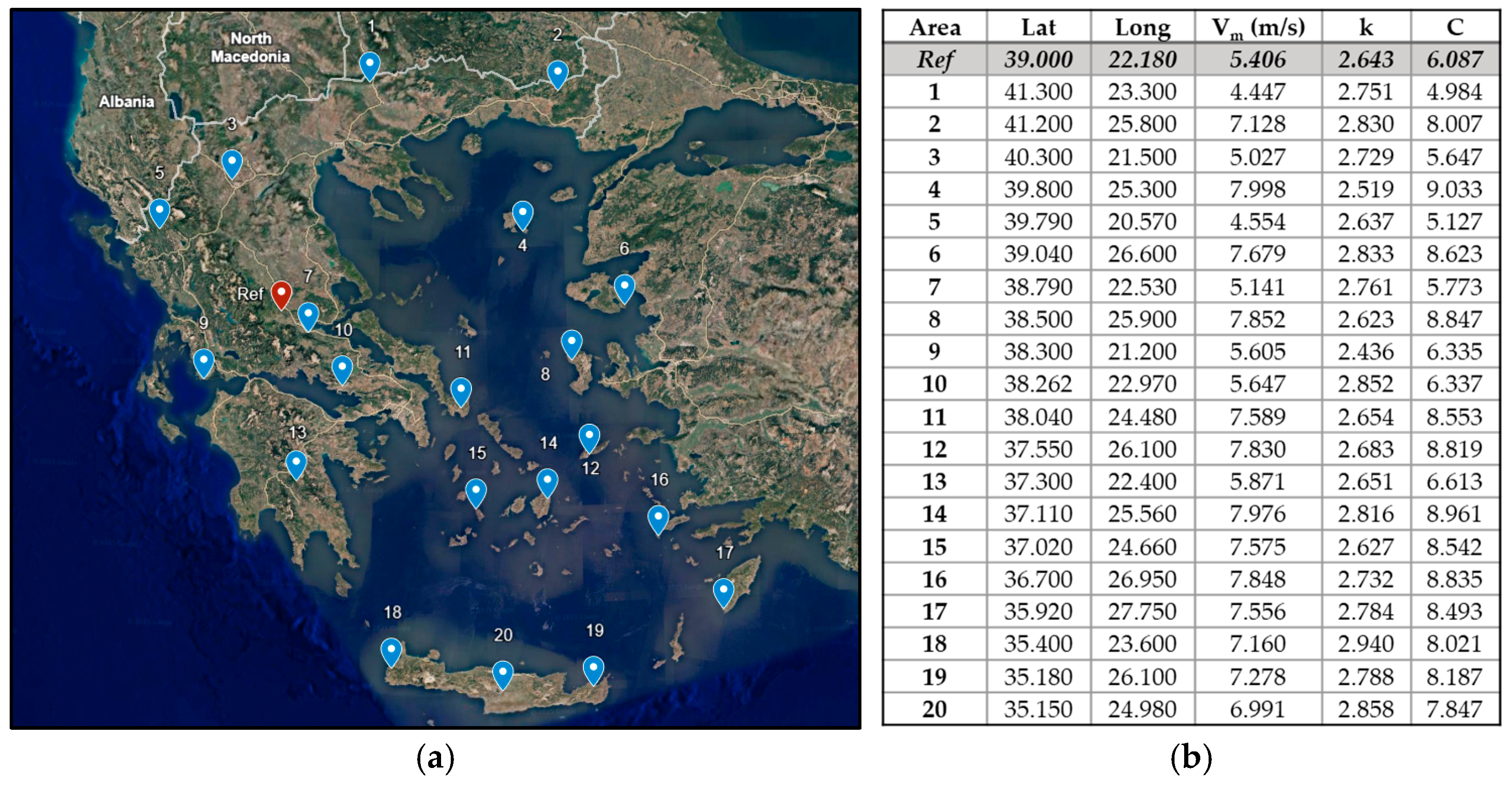
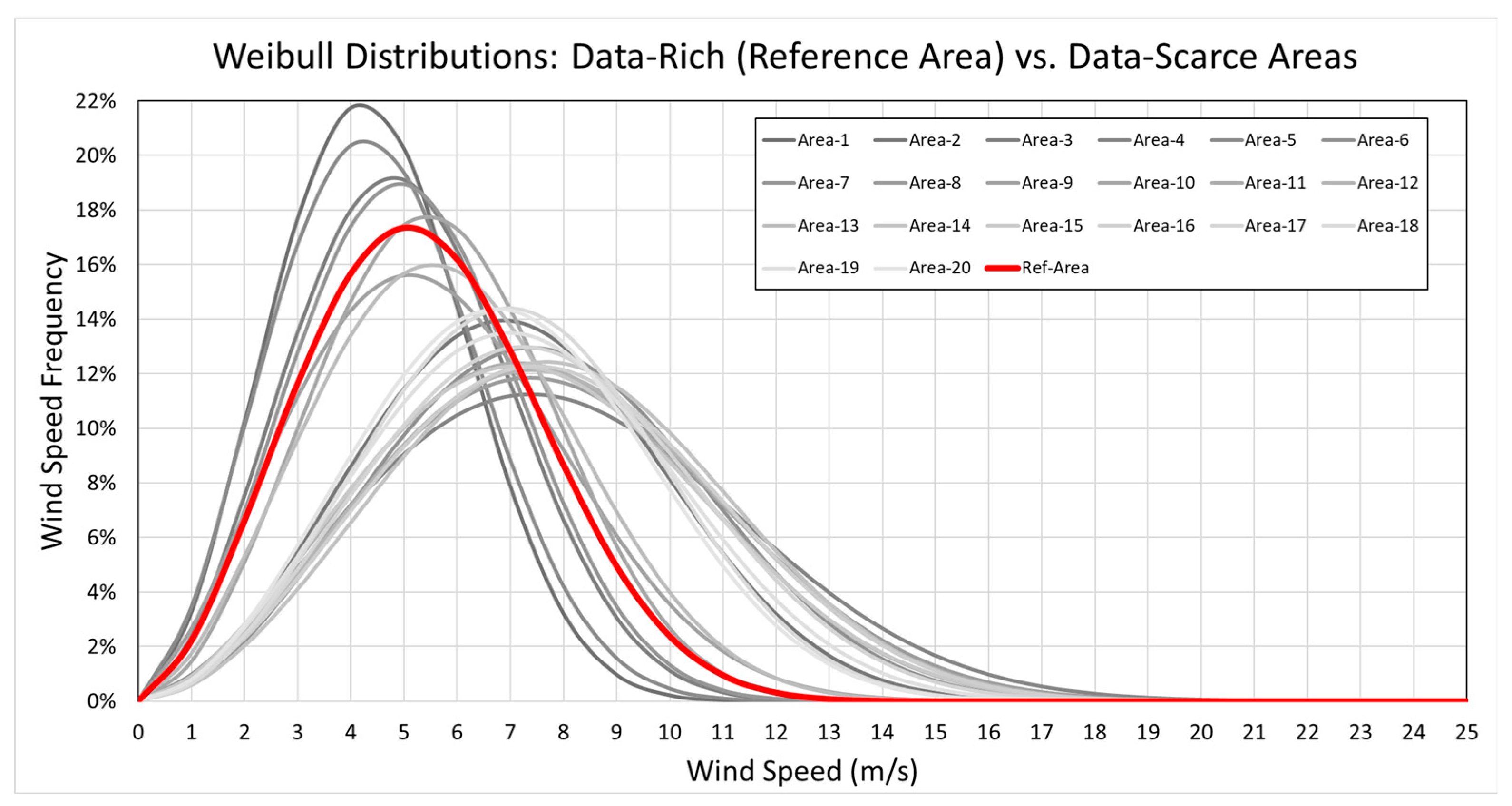
For this study, a vast time-series dataset was exploited. This allowed the examination of broadly different wind potential cases, which essentially reflects on the different wind regimes noted between the Greek mainland and the Aegean Sea (Figure 1 and Figure 2). In more detail, we made use of open-source meteorological data (wind speed at hub height, air temperature, and air density) at a scale of 0.625° × 0.5°, available from the reanalysis MERRA 2 model [18], and applied different dataset time horizons for the data-rich reference area (12-year dataset of hourly values) and the data-scarce assumed geographical locations (1-year dataset of hourly values for twenty areas in total—Figure 1), adopting a hub height of 80 m.

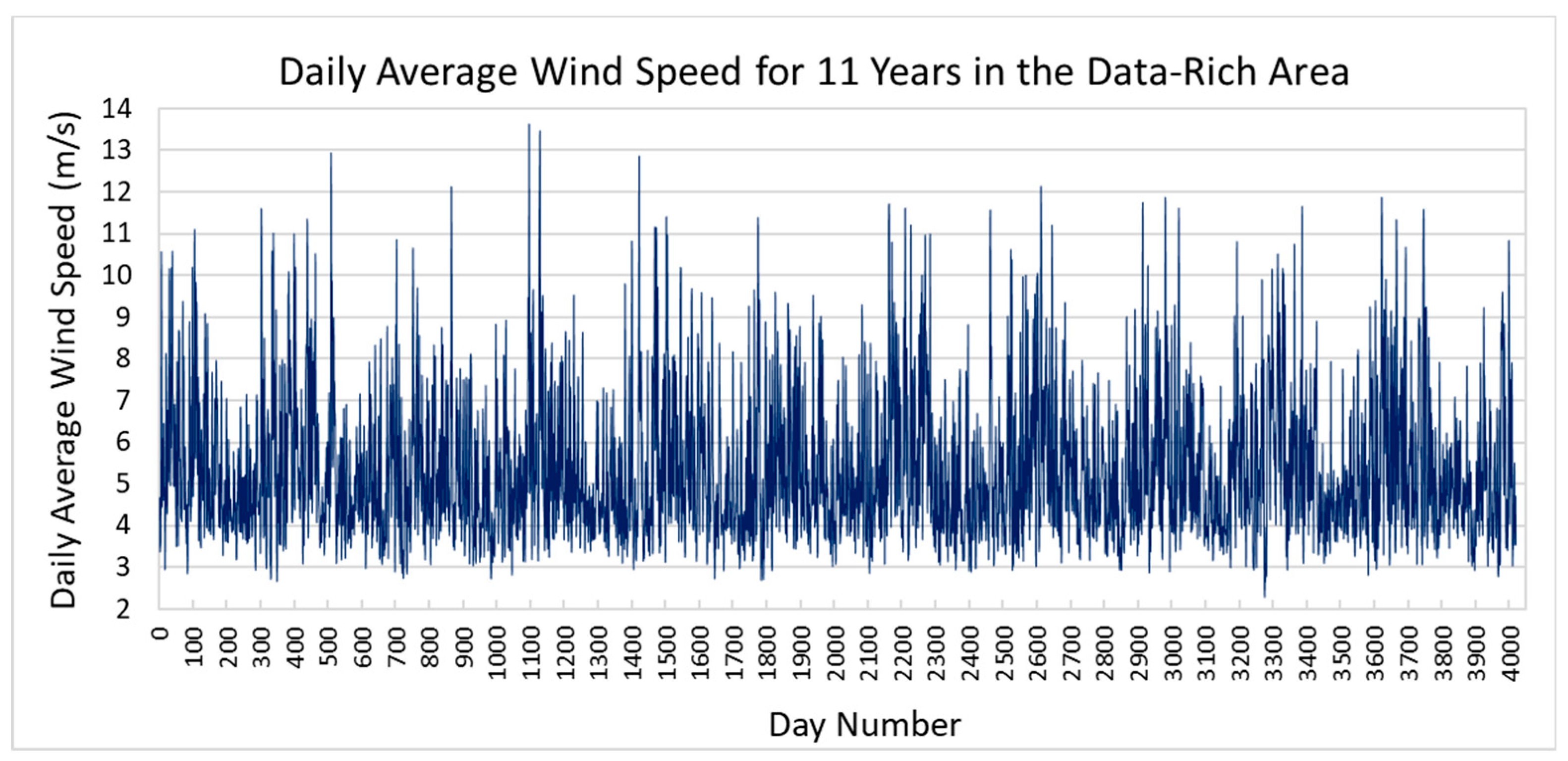
More specifically, the data-rich area features a dataset that spans from 2012 to 2023, following the Coordinated Universal Time (UTC) standard, and includes a total of 105,192 data points in each column, while, for the rest of the areas, the time span is limited to 2023 alone. The first 11-year period, selected to capture long-term interannual variations at affordable computational costs, was used for model training (see also Figure 3 for the relevant daily average wind speed values), while, to assess the predictive performance of the model, the year 2023 was used for all examined areas, including the reference one (

Table 1. Training and testing datasets (raw features).

Dataset	Columns Before Preprocessing
Training—11 years (96,432 data points)	4 (daytime, hub-height wind speed, temperature, air density)
Testing—1 year (8760 data points)	4 (daytime, hub-height wind speed, temperature, air density)

). As such, the evaluation dataset contains 8760 data points, recorded at 1-h intervals. The preprocessing steps applied to the testing datasets mirrored those used during model training, ensuring consistency and readiness for prediction.

Due to the nature of time-series data, six time-related features were generated in order to assist in capturing potential patterns and periodicities. These are presented in

Table 2. Time features and theoretical wind power.

Initial Data	Preprocessing Method	Final Feature
Hour	Sin and cos transformations of hourly periods to preserve cyclical nature	Sin hour, Cos hour
Day	Sin and cos transformations of daily periods across each year	Sin day, Cos day
Month	Sin and cos transformations of monthly periods across each year	Sin month, Cos month
Density of air (ρ), rotor swept area (A), and cube of wind speed (V3)	$P=0.5·\rho ·A·V^3$	Theoretical wind power (P)

. The processing of time-based data often involves extracting features that capture temporal patterns, which are not explicitly apparent in raw timestamps [19]. Cyclical representations of the time features were created for the 11-year dataset, as this method preserves the continuity of periodic variables like hours, days, weeks of year, months, and years.

In the context of this study, for hours, days, and months, sine and cosine transformations were applied, a common approach in time-series modeling so as to handle the circular nature of these variables. For instance, midnight and 23:00 p.m. are close to each other, and without this transform, a machine-learning model might not be able to capture this cyclical relationship. In the same context, a seventh feature was also created, corresponding to the estimated theoretical wind power available (see also Table 2).

Finally, as far as the model target output is concerned (i.e., wind turbine power), the theoretical power curve of a commercial wind turbine was incorporated, which associates wind speed to the wind turbine power output. The wind power curve was obtained from the turbine’s specifications, indicating the anticipated power output at different wind speeds. The wind turbine used was a Vestas V60 (2000 kW), determined by a cut-in wind speed of 3 m/s and a cut-off wind speed of 24 m/s, with its characteristics used in both training and testing datasets.

At this point, it should be noted that the given wind turbine does not necessarily stand as a best-fit solution across all areas examined and that, amongst them, both very low- and very high-quality wind potential cases are present, thus challenging model performance in a broad space of investigation (see also values of mean annual wind speed V_m and relevant Weibull parameters, k and C, for each of the areas—Figure 1 and the corresponding Weibull curves in Figure 2).

2.2. Wavelet Transform and Methodological Framework Overview

In time-series data analysis, accounting for inherent noise that can obscure underlying patterns is crucial. For a non-stationary signal like wind speed, which exhibits significant variability due to atmospheric flow dynamics, a signal processing technique that effectively captures local spectral characteristics of time-varying signals is essential.

Wavelet transform (WT) has emerged as a powerful hybridization approach when combined with various machine learning and deep learning models. It decomposes a complex signal into smaller components across different frequency–time scales, allowing for the extraction of features with varying resolutions, especially in the temporal domain. These derived signals subsequently serve as inputs for various prediction models [20], deeming WT suitable for forecasting in dynamic environments like wind power generation [21].

The fundamental concept of WT is to decompose a signal into different levels of resolution, known as multiresolution analysis. This decomposition allows for the extraction of both low-frequency trends and high-frequency transient information, which can prove to be significant in forecasting. Mathematically, the most general form of wavelet analysis is given by the continuous wavelet transform (CWT). For a signal x(t), the formula for the continuous wavelet transform is as follows:

$$W(a,b)={\int }_{-\infty }^{+\infty }x\left(t\right){\psi }_{a,b}^{*}\left(t\right)dt$$

(1)

where

• ψ*a,b is the wavelet function scaled by a (scale factor) and translated by b (time shift);
• a controls frequency resolution, with higher values corresponding to lower frequencies;
• b determines the time localization of the wavelet;
• * denotes the complex conjugate.

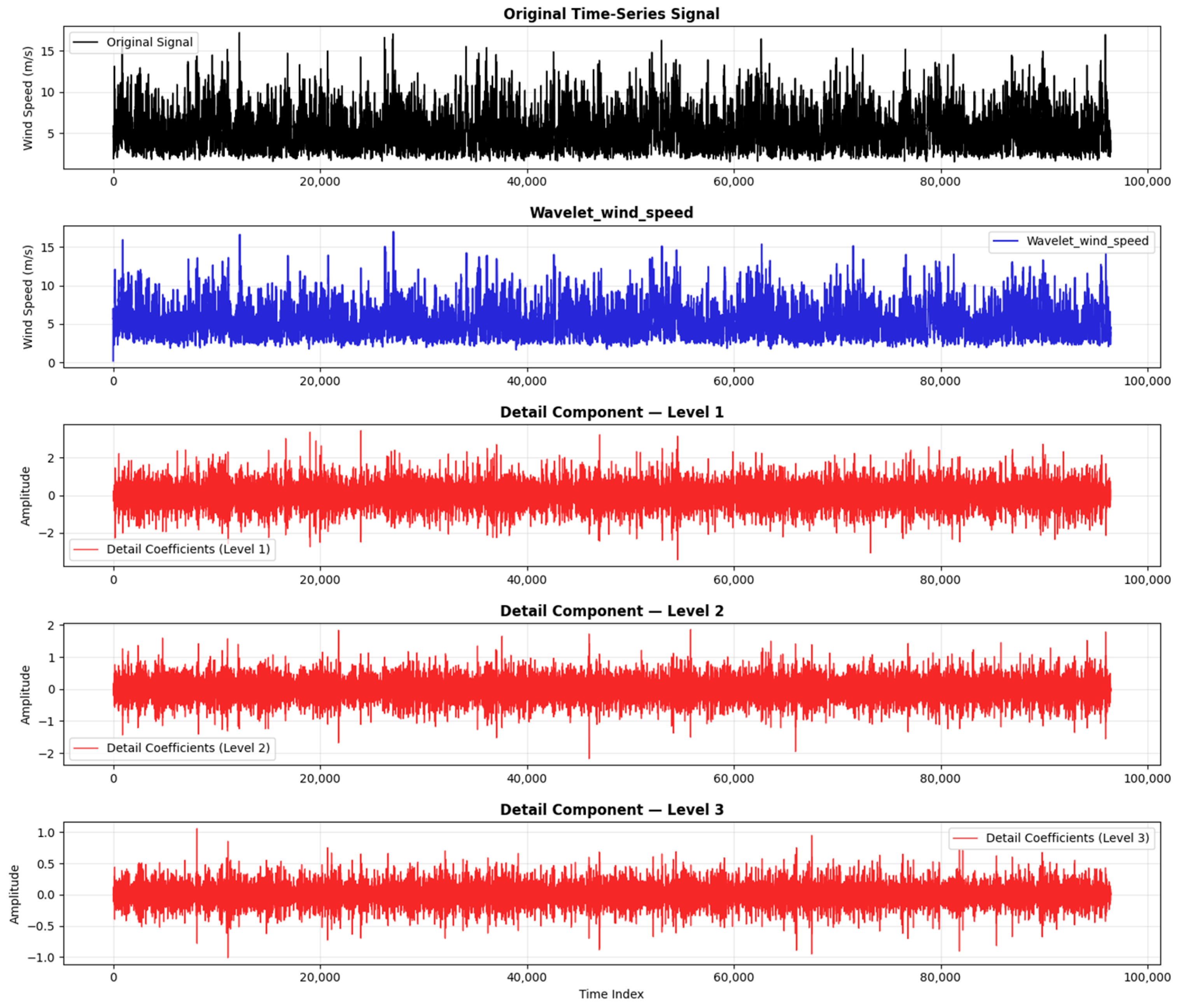
While CWT provides a rich representation of the signal, it is computationally intensive and results in a highly redundant representation. Therefore, for practical applications, a discretized version of the transform—namely the discrete wavelet transform (DWT)—is often used [22]. DWT preserves the main idea of multi-resolution decomposition, but achieves it through dyadic scaling and translation, making it computationally efficient. DWT decomposes a signal into approximate coefficients and detailed coefficients, using a series of filtering operations, and comprises the technique used in the current research (see also Figure 4) as follows:

$$x\left[n\right]=\sum _k{\alpha }_k{\phi }_k\left[n\right]+\sum _k{d}_k{\psi }_k\left[n\right]$$

(2)

where

• ${\phi }_k\left[n\right]$ represents the scaling function, which extracts coarse information;

• ${\psi }_k\left[n\right]$ represents the wavelet function, which captures finer details;

• ${\alpha }_k$ are approximation coefficients that retain the long-term trend of the signal;

• $d_k$ are detail coefficients that highlight fluctuations or short-term variations.

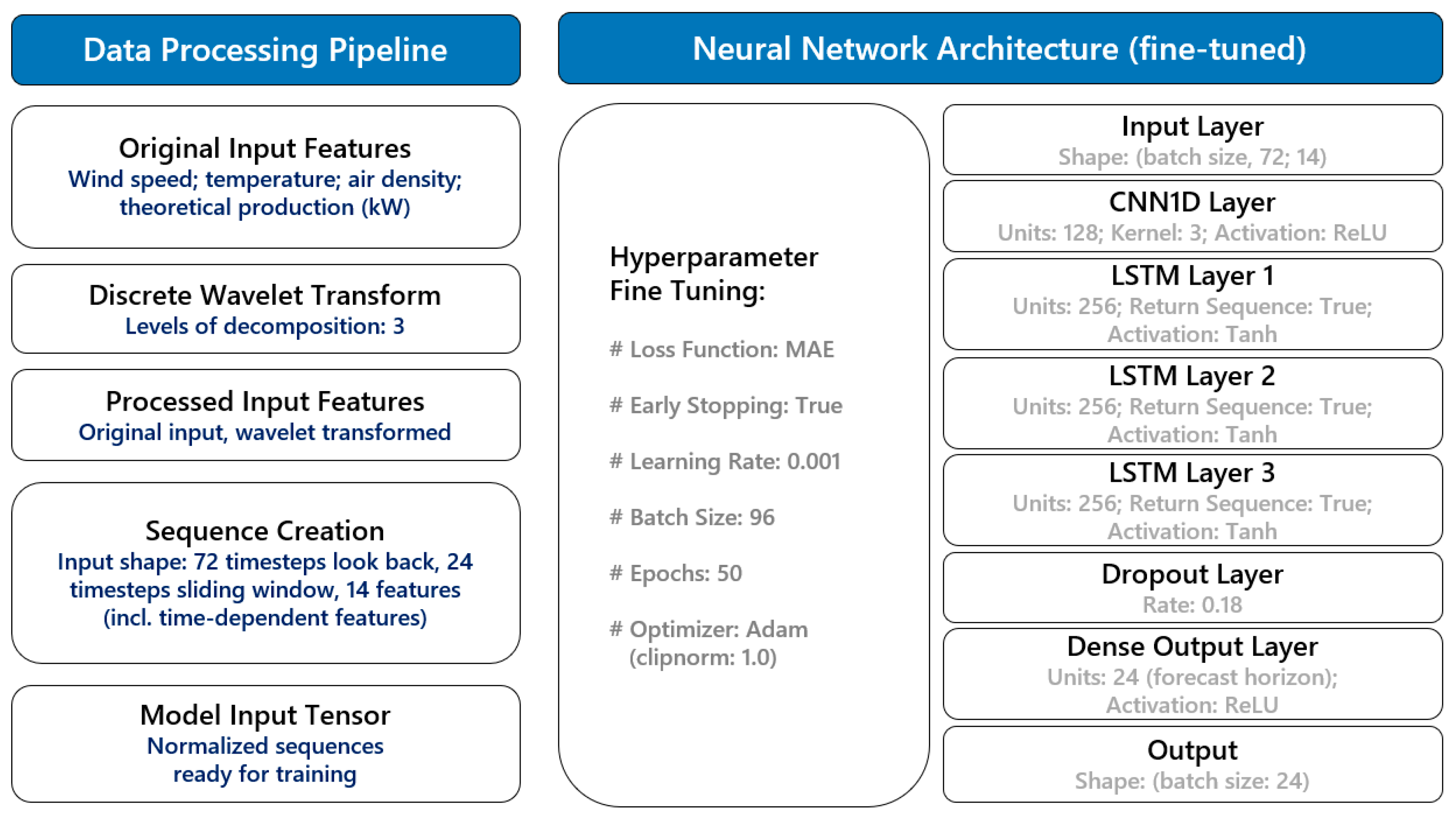
In more detail, DWT was applied across all non-time-based features (hub-height wind speed, air temperature, air density, and theoretical wind power), which were then fed into the CNN-LSTM. This is better illustrated in the data of

Table 3. Final model architecture workflow.

Data Inputs	Preprocessing	Model	Target Window
14 (all except for daytime)	Time feature engineering, Theoretical power generation, DWT	Fine-tuned CNN-LSTM model (for 14 inputs)	24 values of generated power

, also contextualized in the overall methodological framework currently applied, as presented in Figure 5.

The block diagram given in Figure 5 details the components of the data processing pipeline, together with the architecture of the forecasting model developed, aspects of which are further analyzed in the following sub-sections of the paper, i.e., Section 2.3, Section 2.4, Section 2.5 and Section 2.6.

2.3. Sliding Window and Look-Back Period

The sliding window technique is a very effective method used in time-series forecasting. It is usually applied in recursive forecasting models, where future values are predicted based on past data. In the frame of wind power forecasting, the sliding window approach involves a fixed number of past data points as input features for predicting the next value in the series. Wind power is directly influenced by wind speed patterns that span multiple hours, and using a sliding window allows the model to consider these patterns explicitly. The look-back period is a critical parameter that can be tuned based on the specific characteristics of the wind turbine and local weather conditions. A longer window might help capture seasonal trends or longer cycles, while a shorter window is more suited to short-term variability. By providing a fixed-size window of past data, the model can learn the patterns and trends to make accurate forecasts for the future. In this research, direct forecasting was applied, with a look-back period of 72 h and a sliding window of 24 h. The direct forecasting approach involves training a model specifically for a forecasting horizon, unlike the recursive approach, where predictions are used as inputs for subsequent predictions. This means that a dedicated model is trained for each prediction step, such as forecasting wind power output for hour t + 1 h, t + 2 h, and so on, without relying on intermediate predictions.

2.4. Hyperparameter Tuning

In developing deep neural networks, determining the optimal combination of hyperparameters is a crucial step that directly affects the model’s performance. Hyperparameters are configuration variables set before the learning process begins, and they govern various aspects of model training, including network architecture, learning rates, and the size of mini-batches. Finding the best set of hyperparameters is crucial because they significantly influence both the convergence of the training process and the model’s generalization ability on unseen data. Hyperparameter tuning is the process of finding the best hyperparameter values for a model. Some common hyperparameters include the number of neurons, which controls each layer’s capacity to represent complex patterns. Too few neurons may result in underfitting, while too many can lead to overfitting. Another hyperparameter is the batch size, which is the number of samples the model processes before updating the weights. Having a smaller batch size leads to more frequent updates, while a larger one provides smoother gradients but slower training. Learning rate is a critical hyperparameter that controls how much the model’s parameters are adjusted with each update. A learning rate that is too high can cause the model to converge too quickly to a suboptimal solution, while a learning rate that is too low can slow down the training process. Lastly, the dropout rate is a regularization hyperparameter that prevents overfitting by randomly turning off a proportion of neurons during training. In the search for the best combination of these hyperparameters, various techniques can be employed, such as grid search, random search, and more sophisticated methods, like Bayesian optimization or Hyperband. In this study, an Optuna search was applied to automate the process of finding the best configuration based on predefined metrics, resulting in the final models for this research. The bundle of parameters eventually adopted corresponded to 128 neurons for the input CNN layer and 256 neurons for each of the hidden LSTM layers, with a learning rate of 0.001 and a dropout rate of 0.18.

2.5. Optimizers

Optimizers are algorithms or methods that adjust the weights of the neural network to minimize the loss function during training. The choice of optimizer has a direct impact on how quickly the model converges and how well it generalizes to new data. The target of the optimizer is to find the global or near-global minimum. Several optimizers are commonly used in deep learning, each with its advantages and disadvantages. The optimizers that were tested in the context of this study are the following:

• Stochastic Gradient Descent (SGD): One of the most basic optimizers, SGD updates the model’s weights by calculating the gradient of the loss function with respect to the parameters using only a small batch of data. Although SGD is often seen as a simple and effective optimizer, it can prove slow in converging and may also become stuck in local minima.
• Adam (Adaptive Moment Estimation): A more advanced optimizer that combines the benefits of both SGD and momentum-based methods. Adam adjusts the learning rate dynamically by keeping track of past gradients, which leads to faster convergence. It is widely used because of its ability to handle sparse gradients and its robustness across different tasks.
• RMSprop (Root Mean Square Propagation): RMSprop also adapts the learning rate based on the magnitude of recent gradients, making it suitable for problems in which the gradients vary widely across parameters.
• Nadam (Nesterov-accelerated Adaptive Moment Estimation): An extension of Adam, Nadam incorporates Nesterov momentum, which helps improve the optimizer’s convergence speed by looking ahead at the gradient direction. The given optimizer combines the benefits of adaptive learning rates from Adam and the acceleration from Nesterov momentum, making it effective in handling noisy gradients and offering faster convergence.

Choosing the right optimizer is essential because it affects the model’s ability to converge efficiently. A poor choice may result in slow training, oscillating gradients, or even divergence. To find the best working optimizer for a specific task requires a trial-and-error process; this is the reason that the deployment of automated mechanisms is pivotal, in order to find the best-suited optimizer and, by extension, the best-fitting hyperparameters. In this context, the optimizer eventually adopted in this study was Adam.

2.6. Activation Functions

Activation functions are crucial components in neural networks, as they define the output of each neuron. The purpose of an activation function is to introduce non-linearity into the network, enabling it to model complex relationships in the data. Without activation functions, the network would behave like a linear model regardless of its depth, limiting its capacity to solve non-linear problems. There are several widely used activation functions, each suited to different types of tasks and architectures. In this study, the following activation functions were used:

• ReLU (Rectified Linear Unit): ReLU is perhaps the most commonly used activation function in deep learning models nowadays. It works by outputting the input directly if it is positive; otherwise, it returns zero. This simple non-linearity helps to introduce sparsity into the model, allowing only a fraction of neurons to be active at any given time. This sparsity makes ReLU very computationally efficient, while its non-linearity allows the model to capture complex patterns. ReLU was used in both the CNN and dense output layers of the model of the current study.
• Tanh (Hyperbolic Tangent): Tanh also squashes input values, but to a range between −1 and 1, which allows for stronger gradient signals than the sigmoid function. Tanh is typically used in cases for which the model needs to output a value that ranges between negative and positive values. However, like the sigmoid function, it is prone to vanishing gradients in deeper networks. Tanh was used in the LSTM layers of the model in the current study.

2.7. Statistical Evaluation Indices

To evaluate the models’ performance, three key metrics were employed.

• Mean Absolute Error (MAE):

$$\mathrm{{\rm M}}\mathrm{A}\mathrm{{\rm E}}={\displaystyle \frac{1}{n}}·{\sum }_{i=1}^n|y_i-\widehat{y_i}|$$

(3)

This metric calculates the average absolute difference between the predicted and actual values. A lower MAE indicates that the model is making predictions that are close to the actual values on average. MAE is particularly useful for understanding the overall error magnitude and is easy to interpret.

• Mean Absolute Percentage Error (MAPE):

$$\mathrm{{\rm M}}\mathrm{A}\mathrm{P}\mathrm{{\rm E}}={\displaystyle \frac{1}{n}}·{\sum }_{i=1}^n{\displaystyle \frac{\left|y_i-\widehat{y_i}\right|}{\left|y_i\right|}}·100$$

(4)

MAPE is expressed as a percentage, making it easier to interpret across different datasets. It measures the accuracy of the model by quantifying the average percentage difference between predicted and actual values. A lower MAPE indicates better model performance, with smaller deviations from the actual data.

• Coefficient of Determination (R²):

$${\mathrm{R}}^2=1-{\displaystyle \frac{\sum _{i=1}^n{\left(y_i-\widehat{y_i}\right)}^2}{\sum _{i=1}^n{\left(y_i-\overline{y}\right)}^2}}$$

(5)

R², also known as the coefficient of determination, represents the proportion of variance in the dependent variable that is predictable from the independent variables. An R² equal to 0 indicates that the model explains none of the variability, and an R² equal to 1 indicates that the model explains all of the variability.

3. Application Results

3.1. Forecasting Model

Following the description of our methodology, in the current section, we present application results of our research. First, we provide a performance comparison between the simple and DWT-based versions of the hybrid forecasting model developed, using the year 2023 (testing period) and the reference area of study. To that end,

Table 4. Statistical evaluation indices.

Model	MAE (kW)	MAPE (%)	R2
predictions_simple	182.8	129.9	0.514
predictions_wavelet	131.9	76.1	0.734

gives an overview of statistical evaluation metrics, with the MAE, MAPE, and R² values of the DWT-enhanced model outperforming the respective values of the simple model. Moreover, Figure 6, Figure 7 and Figure 8 offer a more comprehensive view of the two models’ performance.

In more detail, Figure 6 presents a time-series comparison between the observed and predicted values for the simple and DTW-enhanced models, respectively, reflecting on the improved performance of the latter.

Models’ performance over time is better perceived in Figure 7, where the span of residuals becomes much narrower in the case of the DTW-enhanced model, with both models, however, determined by an overall, slight underestimation of the anticipated wind power. Season-wise, autumn and winter months feature higher wind power and residual values. The opposite holds true for the summer period (June–July), during which wind power generation minimizes.

Finally, Figure 8 provides linear regression scatter plots between the observed and predicted values, with results indicating broader scattering in the area of 500 kW to 1000 kW of wind power output.

3.2. Spatiotemporal Analysis

Under the given section, spatial forecasting results are presented in the form of a mapping exercise, extending in three different dimensions, i.e., quality of the local wind potential, geographical dispersion, and forecasting horizon. All three dimensions are treated in comparative fashion against the results of the reference location and on the basis of the three statistical evaluation indices applied (MAE, MAPE, R²).

More precisely, the quality of the local wind potential is measured by means of the scale and shape factor of the Weibull distribution, and expressed in the form of differentials ΔC and Δk in relation to the C and k values determining the reference area, with positive values suggesting increases in both C and k. Geographical dispersion, on the other hand, takes consideration of differences in longitude and latitude, with the introduction of ΔLong and ΔLat, respectively.

Lastly, the forecasting horizon dimension provides model performance insights over the hourly course of the 24-h forecasting period in aggregate, i.e., for the entire set of sites examined, assessing the model performance sensitivity per hour of the day together with relevant trends. In this context, mapping of spatiotemporal forecasting results is undertaken in the three following sub-sections, organized per statistical evaluation metric applied.

3.2.1. Mapping of MAE Results

Mapping of MAE results is primarily illustrated in Figure 9. In the first contour plot (Figure 9a), the geographical dimension is examined. Two main distinct areas of MAE variation can be identified to that end, corresponding to the Greek mainland (left side of the plot) and the Aegean Sea region (right side of the plot) (see also Figure 1). Model performance varies significantly between these two areas, indicating that, as we move to the eastern area of the Greek territory, application of the DWT model tends to generate higher values of MAE, also associated with the admittedly higher-quality wind potential of the given region [23].

This becomes more intense for limited latitude differences (ΔLat between 1 and −2.5 degrees), under which MAE values may even exceed 350 kW. On the other hand, the northwestern region of the Greek mainland demonstrates the lower values of MAE, which also links to local wind potential characteristics. The dependence of MAE variation on wind potential characteristics is better seen in the second plot (Figure 9b), looking at the dimension of wind potential quality, using ΔC and Δk. Again, we can identify two distinct areas—and an intermediate layer—of MAE variation, with locations demonstrating that higher values of ΔC also introduce higher values of MAE, consistent with mapping results in Figure 9a. On the other hand, variation in MAE against the variation in Δk presents lower levels of sensitivity, deeming ΔC as more critical concerning the spatial performance of the forecasting model.

Accordingly, variation in MAE values is plotted over the course of the day-ahead forecasting horizon, in aggregate and for all sites examined. Results are given in the form of hourly box plots, also with a clear indication (red markers) of the average hourly MAE values corresponding to the reference area (Figure 10). As it may be obtained from the figure, there is a consistent trend, followed by both the reference area and the general model performance. In more detail, an upward trend is initially noted for MAE values (up to the 4th hour of the day, followed by a slight reduction for the next four hours. From that point onwards, MAE presents a more pronounced increase, resulting in an asymptotic trend over the last six hours of the day. Variation-wise, the relevant ranges appear wider between 15.00 p.m. and 6.00 a.m., with inter-site differences becoming limited between 7.00 a.m. and 14.00 p.m. At the same time, values concerning the reference area are positioned between minima and the 25th percentile, reflecting on the higher performance and previous training of the forecasting model for the given area.

3.2.2. Mapping of MAPE Results

Results concerning the variation in MAPE present considerably different patterns. In terms of geographical dispersion (Figure 11a), higher MAPE values are noted across the Greek mainland territory, on the left side of the plot, also driven by two distinctively higher values for sites No. 5 and No. 10. On the other hand, MAPE reduces considerably in the Aegean region; thus, an inverse behavior emerges, contradicting the variation in MAE. The patterns in relation to the variation in ΔC and Δk (Figure 11b) are also similar. Increase in the former signals a reduction in MAPE, opposite to the case of MAE; meanwhile, with regard to the variation in Δk, MAPE appears to carry increased sensitivity for ΔC values between −0.5 and 1.0.

Accordingly, MAPE variation over the course of the day (Figure 12) follows a similar pattern to the one exhibited in the case of MAE, differing however in terms of variation range, with a higher sensitivity during morning and midday hours (9.00 a.m. to 13.00 p.m.). At the same time, reference values of MAPE are for the biggest part of the day positioned around the 50th percentile, which suggests that the model is able to generate more accurate prediction results for a significant share of sites and span of day-hours.

3.2.3. Mapping of R² Results

Finally, we conclude the presentation of our results by mapping the impacts of key parameters’ variations on the index of R². Similar to the rest of the indices, variations in key parameters entail differentiation of R², depicted in Figure 13 and Figure 14. In terms of geographical dispersion (Figure 13a), the Aegean region is determined by lower values of R², in the range between ~0.56 and ~0.65, while the Greek mainland sites present improved performance, with the reference area determined by a maximum R² value of ~0.73. To that end, higher values of ΔC (>1.5) feature lower values of R², in the range between ~0.56 and ~0.65, while lower ΔC sites feature greater R² values, with the reference area determined by a maximum R² value of ~0.73. Variation in Δk, on the other hand, seems to generate less significant differences (Figure 13b).

Moreover, variation in R² presents a different pattern over the course of the 24-h forecasting horizon (Figure 14). For the first 8 h of the day, R² remains high, exceeding 90%, while, from that point onwards, a decreasing trend is noted as the forecasting horizon extends, with the last quarter of the day presenting values below 40%, and even dropping to 20%.

Interestingly, the given result is found to be largely consistent with the findings of recent research in the field [24], suggesting that high accuracy is demonstrated for the first 6 h of the day, with a gradually decaying trend noted as the time horizon becomes more distant against that time point.

4. Discussion and Conclusions

In the current study, we explored different aspects of spatiotemporal forecasting dynamics, mapping the performance of a hybrid DWT-enhanced forecasting model. The model was trained on rich, long-term, historical data of wind power from a given location on the Greek mainland (central Greece), and was then used in order to test the hypothesis of sufficient day-ahead forecasting performance under its application in data-scarce areas across the broader Greek territory.

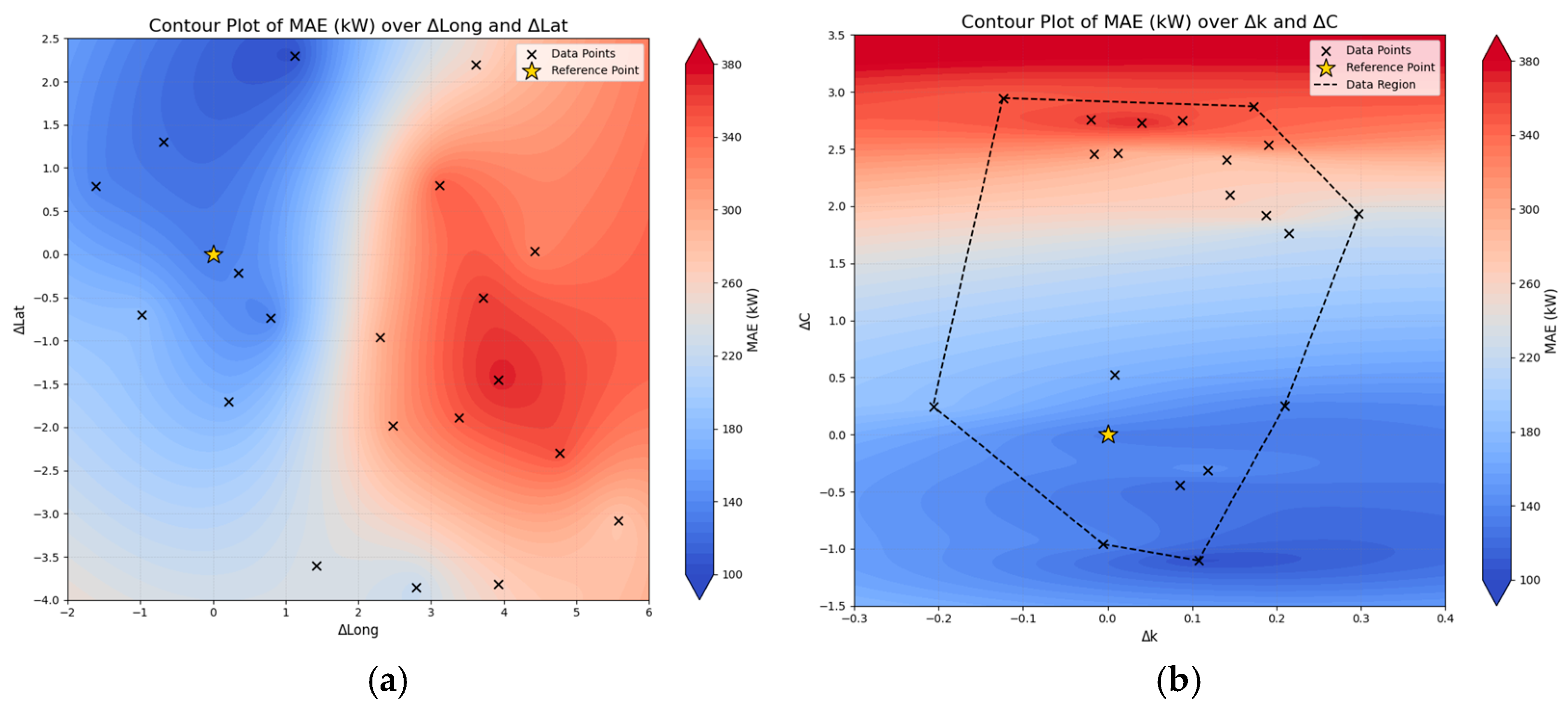
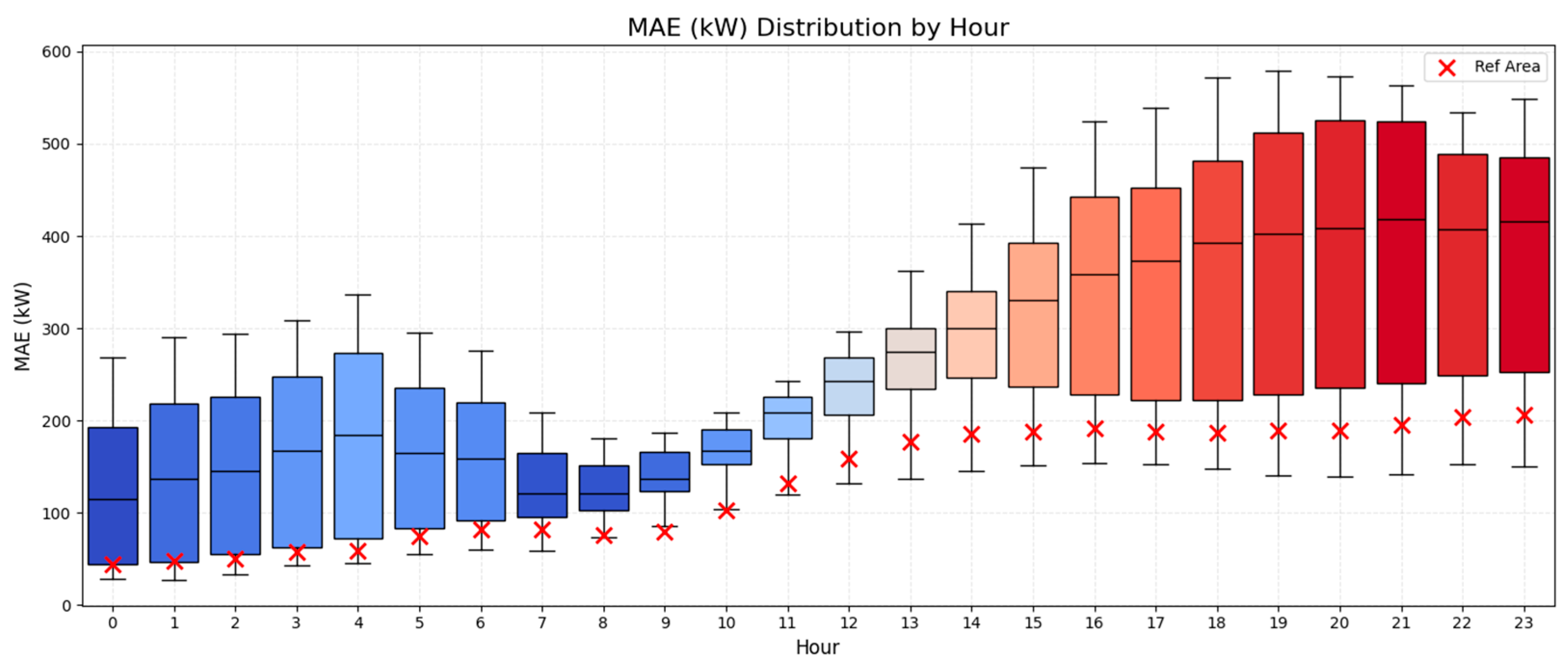
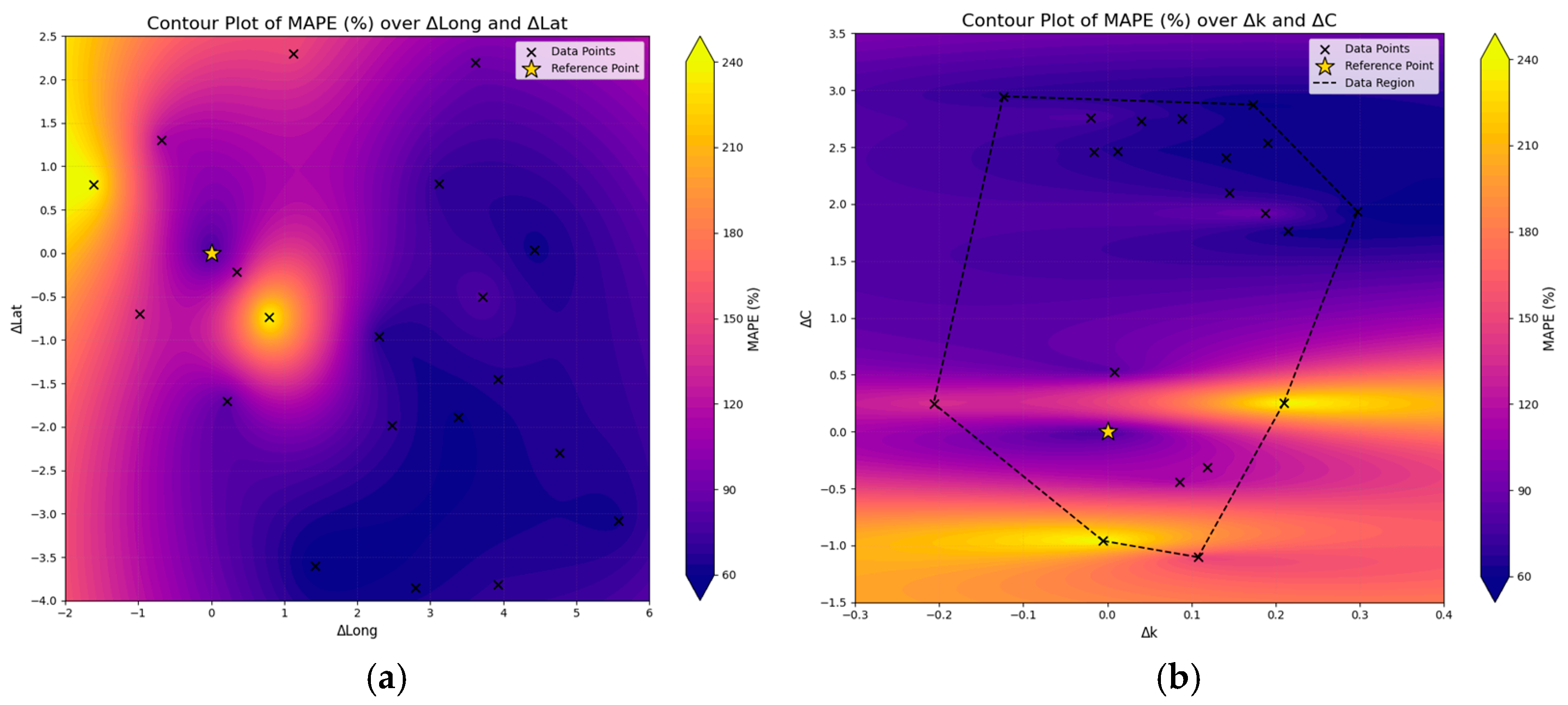
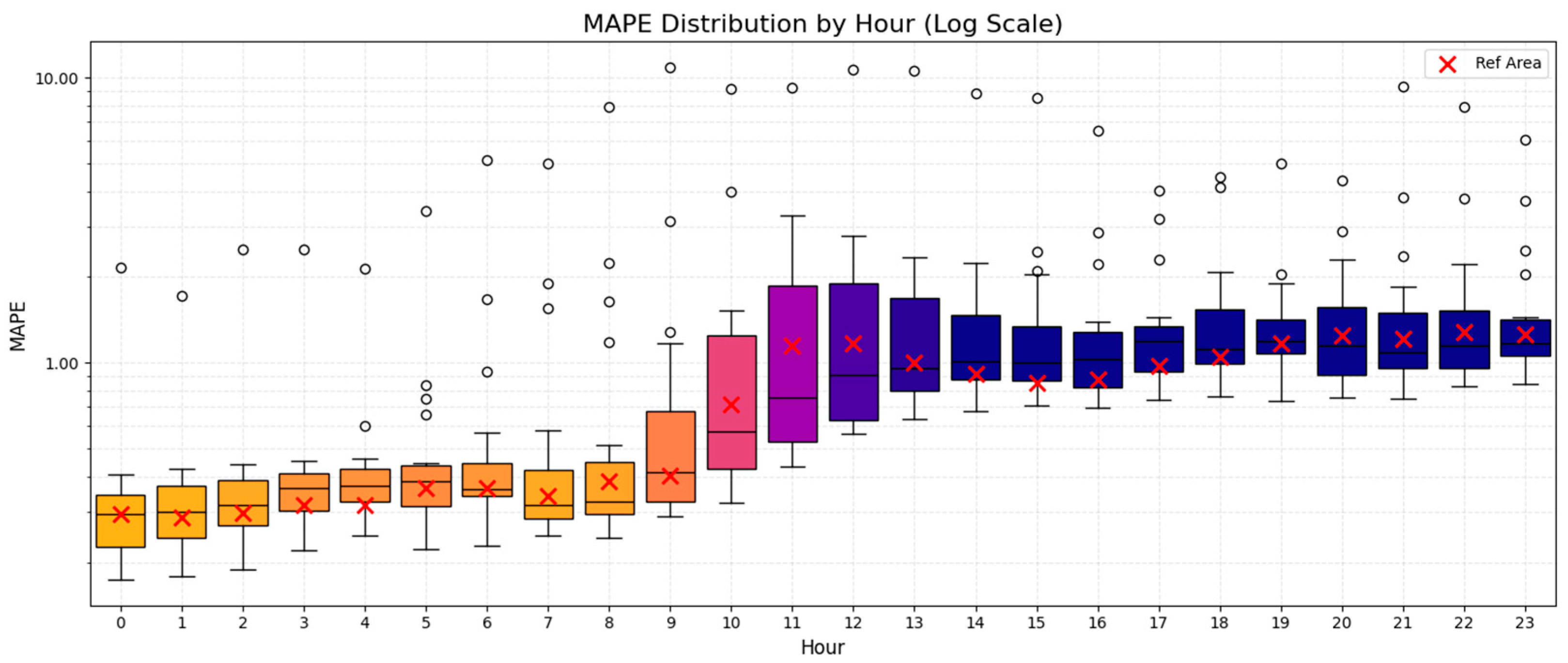
The analysis encompassed three problem dimensions, i.e., the spatial dimension, the temporal dimension, and also a third dimension considering local wind potential characteristics, relying at the same time on three key statistical indices, i.e., MAE, MAPE, and R². The spatial and wind potential dimensions were approached in the context of an annual evaluation regarding the estimation of relevant indices, while the temporal one provided more detailed insights on the performance of the model, further disaggregating results over the 24-h period of the day-ahead forecasting horizon.

Our analysis to that end designated the emergence of two main regions for which the model presented different patterns of performance. The first region corresponds to the Greek mainland, where the area used to train the model is also located, and the second region refers to the Aegean Sea. This geographical distinction also coincides with the establishment of two regions carrying different wind potential characteristics. The Aegean Sea appreciates high- and very high-quality wind potential, while the same is not valid for the most part of the Greek mainland.

To that end, MAE presented itself to be quite higher in the case of the Aegean Sea region, driven by the higher-quality wind potential, while, in the case of MAPE, an inverse behavior was noted, demonstrating that the model performs more efficiently in higher-quality wind potential areas with regard to the given metric. The coefficient of determination (R²), on the other hand, was consistent with the trends noted in MAE, exhibiting lower levels of fitness for the Aegean Sea area. While the model presented different patterns of performance, especially between the two main regions identified, its overall performance can be deemed as sufficient, showcasing its capacity to capture the dynamics of wind potential variation over the broader geographical area of Greece.

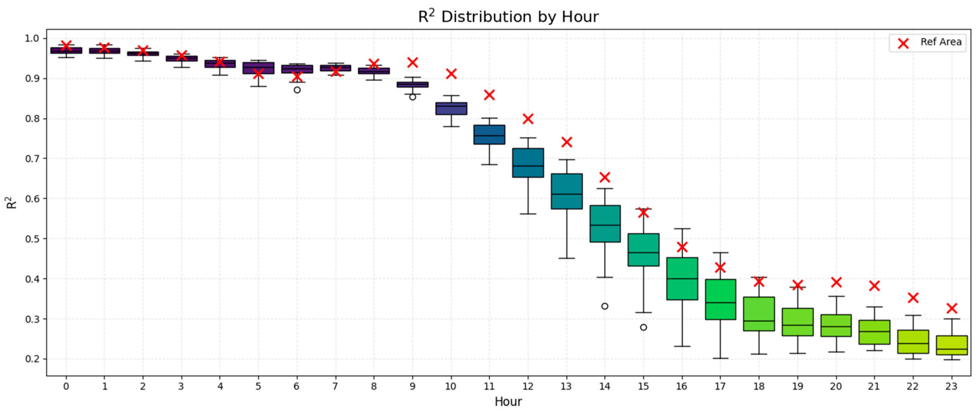
With regard to the temporal dimension of the problem, our analysis designated different patterns of variation over the 24-h forecasting horizon. MAE and MAPE behaved in a similar fashion, with the relevant values presenting an increase in the course of the day, while demonstrating a somewhat stabilizing trend over the last quarter of the day. Uncertainty, perceived as the spatially-driven variations in indices within the pool of examined areas, minimized for MAE and maximized for MAPE, around noontime hours. The coefficient of determination, on the other hand, exhibited higher uncertainty during afternoon hours, with an intense decreasing behavior over the entire 24-h span of the day. At the same time, the model showed high levels of adjustment to the reference area for MAE and R², with MAPE, however, presenting better results for a significant portion of examined areas and time periods over the course of the day.

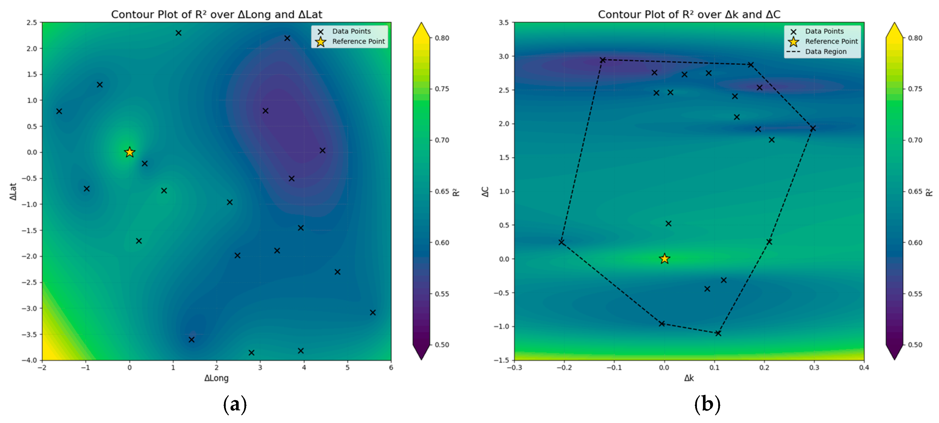
In accordance with the above, the temporal dimension seems to carry a more drastic impact on the model performance. This becomes more pronounced in the case of R² and MAE and fades in the case of MAPE. On the other hand, MAE holds greater sensitivity against wind potential characteristics and is slightly less influenced by the geographical distribution of examined areas, whereas MAPE is largely affected by Δk and, to a smaller extent, by ΔLong. Finally, R² is found to vary within a limited range of values in relation to the spatial and wind potential dimensions during the second half of the 24-h horizon. This is also relevant to the overall model performance, since, according to the temporal dimension analysis, statistical indices present diminishing behaviors past the first 12 h of the day. To that end, and despite being challenged by the presence of regions with highly distinctive wind potential characteristics, it can be argued that, under the assumption of a ~12-h forecasting horizon, the model is able to successfully outweigh the impact of spatial variation at the national level, with limited-only distortions across the Greek territory.

Acknowledging that, application of similar intra-day or shorter-horizon forecasting models suggests a prospective solution that may address the problem of data scarcity in several areas, which, by leveraging data-rich areas for the training of relevant models, may provide firm estimations on the anticipated wind power generation patterns. Furthermore, this also positions our research in the planning domain, adding value to common wind farm design approaches through the application of a deeper analysis that touches upon operational aspects, as well.

Additionally, and in the context of further research, the developed methodology can be evaluated both in a broader geographical context and become validated on the basis of actual operational data from already existing wind farms. By expanding the problem space of our analysis, new dynamics could emerge, while, by challenging the capacity of the proposed approach to provide sufficient forecasting results for actual wind projects, commitment of otherwise necessary training resources and big data availability could be effectively addressed. Beyond that, application of clustering techniques, such as in [25], may lead to a deeper understanding of the model’s performance as far as regional correlation aspects amongst the examined areas are concerned.