Article

Adaptive Sliding Mode Observers for Speed Sensorless Induction Motor Control and Their Comparative Performance Tests

by
Halil Burak Demir
1,
Murat Barut
1,*,
Recep Yildiz
1 and
Emrah Zerdali
2
1
Department of Electrical and Electronics Engineering, Niğde Ömer Halisdemir University, Niğde 51200, Türkiye
2
Department of Electrical and Electronics Engineering, Ege University, Izmir 35040, Türkiye
*
Author to whom correspondence should be addressed.
Energies 2025, 18(20), 5530; https://doi.org/10.3390/en18205530
Submission received: 5 September 2025 / Revised: 7 October 2025 / Accepted: 11 October 2025 / Published: 21 October 2025

Abstract

This paper presents adaptive sliding mode observers (A-SMOs) performing speed estimation for sensorless induction motor drives utilized in both industrial and electrical vehicle (EV) applications due to their computational simplicity. The fact that the constant switching gain ( λ 0 ) is used in conventional SMOs (C-SMOs) leads to the chattering problem, especially in low-speed regions. To tackle this issue, this paper proposes two different λ 0 adaptation mechanisms based on fuzzy and curve fitting methods. To estimate stator stationary axis components of stator currents and rotor fluxes together with the rotor speed, the proposed A-SMOs only utilize the measured stator currents and voltages of the IM. Here, the difference only between the estimated and measured stator currents is determined as the sliding surface in the proposed A-SMOs. To demonstrate the effectiveness of the proposed fuzzy-based A-SMO (FA-SMO) and curve fitting-based A-SMO (CFA-SMO), they are compared with C-SMO in real-time experiments for different scenarios including wide speed range operations of IM with/without load torque changes. Moreover, the stator and rotor resistances as well as the magnetizing inductance variations are also examined in real-time experiments of the proposed methods and the conventional one. The estimation results demonstrate how positively the λ 0 adaptations in FA-SMO and CFA-SMO affect the performance of C-SMO. Finally, two A-SMOs with improved performance are introduced and verified through real-time experiments.

1. Introduction

With the developing technology in recent years, speed sensorless induction motor (IM) control has become increasingly important because of IM’s low cost, widespread use, and advanced drive technology [1]. Depending on the application, the speed sensorless IM drives require the estimation of rotor speed ( ω m ) as well as the stator stationary axis components of stator ( φ s α and φ s β ) or rotor fluxes ( φ r α and φ r β ) [2]. To carry out these estimations, various state observers/estimators have been proposed in the literature such as model reference adaptive systems (MRAS) [3], Kalman filter-based observers [4,5], Luenberger observer [6,7], and sliding mode observer (SMO) [8,9].
Conventional MRAS estimators suffer from the use of pure integrators and performance degradation due to parameter changes. To overcome these problems, different adaptation methods are used in the adaptation mechanism of the MRAS estimators in the literature such as least mean square and least mean Kurtosis algorithms [10]. Furthermore, hybrid structures are used to make MRAS methods robust against parameter variations [11]. Additionally, Kalman filter-based solutions are employed because they can conduct real-time estimations of states and parameters, accounting for system/process errors and measurement noises directly [4]. However, the obvious drawbacks of Kalman filter-based methods are difficulties in implementing them in a digital signal processor (DSP) due to their high complexity [12] and the laborious selection process of noise covariance matrices [13]. On the other hand, considering the extended Luenberger method, the pole-placement process needs to be performed by determining an appropriate gain matrix selection, which can be classified as one of the difficulties of this method [7] together with its sensitivity to changes in IM parameters.
Compared to other estimators/observers detailed above, the advantages of the sliding mode observer (SMO) can be given as low computational load, ease in implementation to DSP, and higher performance against uncertainties [14,15]. As is known, correct determinations of the model parameter values play a key role in the performance of the estimators/observers. Even if the IM parameter values are well determined, the observer and thus control performance may not be satisfying because of the parameter variations caused by the temperature, frequency, and flux level changes [16]. Since SMO is classified as a robust method, various SMO-based studies have been conducted on state/parameter estimation of IMs [17,18,19]. Due to the fact that parameter variations—particularly the stator and rotor resistances ( R s and R r ) in the low-speed region and the magnetizing inductance ( L m ) in the field-weakening region—cause performance deterioration, the rotor speed ( ω m )-estimation performance of SMO has been improved in the literature through the online estimation of these varying parameters. In Wang et al. [20], a second-order SMO is combined by MRAS to perform ω m estimation along with R s estimation. In Mezouar et al. [21], the ω m estimation is performed together with the inverse of the rotor time constant. In Zaky et al. [22], the R s estimation is carried out to improve ω m using SMO-based parallel identification schemes. Moreover, the L m estimation is also performed in the field-weakening region operation. Furthermore, to improve the ω m estimation performance, there are also hybrid structures utilized in the literature, as in Shen et al. [23], which uses a fuzzy dual sliding mode MRAS structure. Together with the advantages of the SMO technique, it also has some weaknesses such as chattering and parameter dependency since it is still a model-based method, and required time to reach the sliding surface. To overcome these problems, many SMO algorithms have been proposed so far, called first [24], high-order [25], and reaching law-based SMOs [8,26].
Given the different SMO algorithms, super-twisting SMO (STSMO) is one of the most well-known high-order SMO methods [9,27,28]. High-order SMOs are generally proposed to solve the chattering phenomenon in the first-order SMOs [29]. However, as stated in Gonzalez et al. [30], STSMOs do not compensate time-varying disturbances/uncertainties if they are designed with constant switching gains. Moreover, to solve chattering problems caused by the nature of conventional SMOs (C-SMOs) as in [24], fuzzy-based algorithms have been developed instead of the signum function used in C-SMOs [31]. Moreover, the sliding mode control law equations of high-order SMOs, such as STSMO, involve a relatively high computational load and include pure integration, as seen in Nurettin and Inanc [9] and Ammar et al. [28]. Additionally, other studies aim to eliminate the chattering components observed at the system output by employing a low-pass filter during rotor flux estimation [24,32]. However, in this case, it causes a delay in speed estimation and an error in amplitude [19]. To solve this problem, a continuous hyperbolic tangent function is used instead of a low-pass filter [33]. Nevertheless, this method only guarantees the convergence of the sliding motion to the sliding surface. Furthermore, the chattering issue still persists due to the high switching gain ( λ 0 ) [19]. Since using a constant λ 0 leads to chattering and performance degradation—particularly in the low-speed region—the value of λ 0 needs to be adjusted based on the operating conditions of IM. In addition to the aforementioned SMO techniques, adaptive SMO (A-SMO) methods that adjust λ 0 dynamically have also been proposed in the literature. A-SMOs have many advantages for speed estimation such as adaptation of switching gain and reduction in chattering problem in low-speed operation [9,18,19,20,25,34,35,36,37,38,39,40]. There are different approaches in the literature related to A-SMOs, which have observer gain adaptations and λ 0 or switching coefficient adaptation. The observer gain is changed depending on the IM parameters and ω m [34,35,37]. When it comes to [9,18,19,25,36,38,39,40,41,42], Keyhani et al. [36] and Tarchala and Orlowska-Kowalska [38] propose a speed-adaptive SMO with a sliding surface defined as a function of stator current ( i s α and i s β ) errors and rotor fluxes. Here, the ω m estimation is performed by multiplying the determined sliding surface and an adaptive λ 0 ; the adaptive λ 0 is obtained using a first-order polynomial of ω m in both studies. In Hu et al. [39], an A-SMO is designed with a sliding surface determined as the stator current errors and the adaptive λ 0 values for each axis ( α and β ) are calculated as a function of IM parameters, the estimated states ( i s α , i s β , φ r α , φ r β , and ω m ), and determined additional gain term. Therefore, the adaptive λ 0 value depends on the IM parameters, which results in the parameter sensitivity. Moreover, the trial and error method-based determination process of the additional gain terms can also be evaluated as a second drawback of the proposed method. In Kousalya and Singh [18], an adaptive STSMO (A-STSMO) is proposed with a sliding surface determined as the stator current errors. The speed-adaptive switching coefficients in STSMO are separately determined as functions of rotor speed and rotor speed squared. In Nurettin and Inanc [9], an A-STSMO with the same sliding surface defined in Kousalya and Singh [18] and Prince and Yoon [27] is proposed. Contrary to Kousalya and Singh [18], four switching coefficients, two for each axis, are used. One of the switching coefficients for each axis ( α and β ) is determined as constant while the other is adaptively calculated. Similar to Hu et al. [39] and Zerzeri et al. [42], the IM parameters, estimated states ( i s α , i s β , φ r α , φ r β , and ω m ), and additional gain term are utilized in the determination of adaptive switching coefficients. In Sun et al. [19], an adaptive nonsingular terminal SMO (A-NTSMO) is introduced with a second-order nonsingular terminal sliding mode surface. Here, a speed-adaptive coefficient is used in A-NTSMO which contains a couple of constant coefficients to be determined. Therefore, the determination process of these constant coefficients can be evaluated as the difficulty of the proposed method. Wang et al. [25] and Bu et al. [43] propose a discrete SMO-based MRAS method with speed adaptation to avoid the chattering problem. The proposed discrete SMO-based MRAS in [25] is compared to existing STSMO-based MRAS with speed adaptation. In Wang et al. [41], a speed-adaptive high-order SMO is proposed to achieve finite-time convergence, and the method is compared with first-order and super-twisting SMOs. Two coefficients of the defined high-order sliding surface are selected as constants. Moreover, λ 0 is obtained as a first-order polynomial, independent of the estimated synchronous speed derived from the high-order SMO-based MRAS. In Bai et al. [40], an adaptive SMO structure that uses a continuous switching function instead of the s n g function to suppress the chattering effect is proposed. In the proposed method, the λ 0 value is determined as the sum of the rotor speed and a constant coefficient, aiming to improve the performance in estimating the rotor speed and position information of the permanent magnet synchronous motor (PMSM). However, the method used in this study to reduce the required time to approach the sliding surface also introduces a pure integration problem.
The main contribution of this paper is to propose two novel A-SMOs to overcome the operation speed region-based performance-deterioration problem of C-SMO as in [24] by changing the λ 0 value. The proposed A-SMOs use only the current errors in the sliding surface, similar to past studies [9,39] but with different adaptive mechanisms that are mathematically simpler and parameter-independent. This reality can be discovered by inspecting the adaptive mechanisms (Equation (23) in Nurettin and Inanc [9] and Equation (20) in Hu et al. [39]) which additionally require the estimated and/or measured states (flux and/or stator currents) and varying parameters (rotor time constant, L m etc.); thus, the proposed adaptive mechanisms in this paper are more convenient than those of past studies [9,39] for real-time high performance control of industrial systems and electrical vehicles (EVs) requiring for speed sensorless drives. For λ 0 adaptation based on the operating speed, fuzzy logic and curve fitting methods are employed in the design of the proposed adaptive mechanisms. The motivation behind selecting these methods is that they introduce only a slight increase in computational load compared to the conventional SMO (C-SMO) [24], while also being parameter-independent and computationally simpler than those used in previous studies [9,39]. Since A-SMO with proposed adaptive mechanisms does not lead to a significant computational load increase, they can easily be used in the high performance control of EV and industrial systems. Therefore, the low-computational load characteristic, one of the most favourable sides of C-SMO [24], is also used in this paper. Moreover, the proposed A-SMOs with the online estimations of i s α , i s β , φ r α , φ r β , and ω m only utilize measured stator voltages ( u s α and u s β ) as well as i s α and i s β . To show the effectiveness of the proposed fuzzy adaptive SMO (FA-SMO) and curve-fitting adaptive SMO (CFA-SMO) methods, they are tested in real-time experiments including wide speed range operation of IM with/without load torque changes. Additionally, the estimation performances of the proposed methods are fairly compared with that of C-SMO through real-time experiments in which all observers operate in parallel at the open-loop condition. Furthermore, to examine the effect of the parameter variation over the proposed A-SMOs and C-SMO, variations in R s and R r are performed in the low-speed region while the L m -change is realized in the high-speed operation. Finally, the obtained experimental results demonstrate the superiority of the proposed λ 0 adaptive methods in this paper over C-SMO. Moreover, the experimental results clearly indicate that the proposed A-SMOs are highly promising candidates for sensorless IM drives utilized in both industrial and EV applications. In summary, the proposed methods in this study (FA-SMO and CFA-SMO) are different from:
  • Nurettin and Inanc [9] utilizing STSMO and its adaptation mechanism sensitive to the parameters and states of IM.
  • Kousalya and Singh [18] exploiting STSMO with the separately determined speed-adaptive two switching coefficients as functions of rotor speed and rotor speed squared, which results in problematic operations at zero speed, making both switching coefficients zero.
  • Hu et al. [39] using C-SMO and its adaptation mechanism sensitive to the parameters and states of IM.
  • Wang et al. [41] employing the high-order SMO defined with a mathematically complex sliding surface and the speed estimation performed by the high-order SMO-based MRAS.
This paper consists of five sections. Section 1 presents the literature review and the contribution of this study. Section 2 presents the dynamic model of IM and C-SMO equations. Section 3 explains FA-SMO and CFA-SMO to perform ω m estimation. Section 4 presents the experimental setup, and shows the real-time results for C-SMO and the proposed A-SMOs to demonstrate the effectiveness of the proposed methods. Finally, Section 5 provides the conclusion.

2. Dynamic Model of IM and Conventional SMO

2.1. Dynamic Model of IM

Three-phase IMs are commonly modeled using a fifth-order nonlinear mathematical representation, under the assumptions of magnetic linearity (i.e., no saturation), negligible core losses, and insignificant effects from temperature and parameter variations. This model is well-suited for state-estimation purposes, as it offers a practical trade-off between computational complexity and estimation accuracy. It can be formulated in either the stationary reference frame ( α β ) or the rotating reference frame (dq). Similar to [8,9,24,27] in this study, the electrical equations of the IM model are expressed in the α β frame, as presented in Equations (1)–(4).
d i s α d t = L m R r σ L m L m 2 φ r α + L m σ L s L r ω m φ r β R s L r 2 + R r L m 2 σ L s L r 2 i s α + 1 σ L s u s α
d i s β d t = L m σ L s L r ω m φ r α + L m R r σ L m L m 2 φ r β R s L r 2 + R r L m 2 σ L s L r 2 i s β + 1 σ L s u s β
d φ r α d t = R r L r φ r α ω m φ r β + R r L m L r i s α
d φ r β d t = ω m φ r α R r L r φ r β + R r L m L r i s β
where L s , L r , and L m are the stator, rotor, and mutual inductances, respectively. u s α and u s β represent the stationary axis components of stator voltages. Furthermore, σ = 1 ( L m 2 ) / ( L s L r ) is the leakage coefficient. Equations (1)–(4) can be represented in the matrix form as below:
d i s α d t d i s β d t = k 1 1 T r ω m ω m 1 T r φ r α φ r β 1 T r L m i s α i s β
k 2 i s α i s β + k 3 u s α u s β
d φ r α d t d φ r β d t = 1 T r ω m ω m 1 T r φ r α φ r β 1 T r L m i s α i s β
where k 1 = ( k 3 L m ) / L r , k 2 = R s / ( σ L s ) , k 3 = 1 / ( σ L s ) , and 1 T r = R r / L r .
The model in (5) and (6) can be defined in the following state-space form.
x ˙ = f ( x , ω r ) + B u y = h ( x )
Remark 1.
The system is said to be locally observable around point x 0 if the observability rank condition is satisfied; that is, the Jacobian of the stacked Lie derivatives with respect to the state vector x has full rank (which is 4 in this case).
The observability matrix O , obtained from the gradients of these Lie derivatives [5], is constructed for the utilized IM model in this paper as follows:
O ( x ) = L f 0 y 1 L f 0 y 2 L f 1 y 1 L f 1 y 2 L f 2 y 1 | | L f 2 y 2 .
where L f 0 y 1 = i s α , L f 0 y 2 = i s β , L f 1 y 1 = d i s α / d t , L f 1 y 2 = d i s β / d t , and L f 2 y 1 | | L f 2 y 2 = function of i s α , i s β , φ r α , φ r β , ω r .
If this matrix has rank 4, the model is locally observable at the corresponding operating point. According to the analysis, when ω r 0 , the Lie derivatives exhibit nontrivial dependence on φ r α and φ r β due to the speed-induced coupling between stator and rotor dynamics. As a result, the Jacobian of the Lie derivatives spans the full state space, satisfying the observability rank condition. In contrast, when ω r = 0 , the Lie derivatives of the output functions fail to capture the full state information, particularly the rotor flux components, thereby rendering the system unobservable at standstill.

2.2. Conventional SMO

Looking at (5) and (6), a common term for current and flux equations stands out. Thus, this common term can be defined as a new matrix (G) as follows;
G = G α G β = 1 T r ω m ω m 1 T r φ r α φ r β 1 T r L m i s α i s β
Since the coupling (common) terms in (5) and (6) between the α - and β -axis are identical, it is possible to define a sliding mode function instead of these coupling terms. Subsequently, the sliding mode function can be employed to perform the estimation of the common terms as given in (9) [8]:
f α f β = G ^ = 1 T r ω ^ m ω ^ m 1 T r φ ^ r α φ ^ r β 1 T r L m i ^ s α i ^ s β
Using the sliding mode function, the current and flux estimations can be performed with the help of (11) and (12). Here “ . ^ ” refers to the estimated state or parameters.
d i ^ s α d t d i ^ s β d t = k 1 f α f β k 2 i ^ s α i ^ s β + k 3 u s α u s β
d φ ^ r α d t d φ ^ r β d t = f α f β
where
f α f β = λ 0 sgn ( S α ) λ 0 sgn ( S β )
sgn = 1 : S α < 0 0 : S α = 0 1 : S α > 0
As is well known, in (13), λ 0 is the switching gain of C-SMO which must be chosen large enough to obtain fast convergence of estimations and the stability of the observer. On the other hand, if a too large λ 0 is used in C-SMO, the estimated states will suffer from the chattering phenomenon. In this paper, it is also observed that the λ 0 value of C-SMO must be appropriately adjusted depending on the operation condition of IM, particularly with respect to the speed region, to enhance the estimation performance [44]. This is the reason why the λ 0 value is modified according to ω m in the proposed A-SMO methods. Finally, the sliding surface is defined as follows:
S α S β = i ^ s α i s α i ^ s β i s β
As seen in (12), flux estimation requires integration of f α and f β values. Due to the signum ( sgn ) function, f α and f β values change between positive and negative λ 0 values, resulting in high-frequency oscillation. In C-SMO, the equivalent control concept is utilized to maintain motion on the sliding surface and reducing the oscillation. For this purpose, the equivalent control term can be obtained as in (16) [39].
f α β e q = 1 μ s + 1 f α β
Here, the time constant ( μ ) of the low-pass filter should be large enough to eliminate high-frequency components and small enough to allow low frequency components of the f α and f β values. After defining the equivalent control term, (10) can be transformed to (17). Putting (17) into (12), then
f α e q f β e q = G ^ = 1 T r ω ^ m ω ^ m 1 T r φ ^ r α φ ^ r β 1 T r L m i ^ s α i ^ s β
Rotor flux estimation can be performed as in (18).
d φ ^ r α d t d φ ^ r β d t = f α e q f β e q
Realizing flux estimation by using (18) has some drawbacks such as DC offset due to a pure integration process. To overcome the DC offset problem and to obtain high estimation performance, a small amount of feedback maintaining the stability of the integral can be used as in [45]. After performing the flux estimation, ω m can be estimated in the C-SMO method. To realize the ω m estimation, row 1 and row 2 of (17) are multiplied by φ r β and φ r α , respectively, resulting in (19), and φ ^ r α f β e q is subtracted from φ ^ r β f α e q . Thus, the resulting equation of ω m can be obtained as in (20).
φ ^ r β f α e q φ ^ r α f β e q = G ^ = φ ^ r β 1 T r φ ^ r β ω ^ m φ ^ r α ω ^ m φ ^ r α 1 T r φ ^ r α φ ^ r β 1 T r L m φ ^ r β i ^ s α φ ^ r α i ^ s β
ω ^ m = φ ^ r β f α e q φ ^ r α f β e q 1 T r L m ( φ ^ r α i ^ s β φ ^ r β i ^ s α ) φ ^ r α 2 + φ ^ r β 2
The expression in (20) can be used to estimate ω m by using i ^ s α β and φ ^ r α β values estimated by C-SMO. However, considering the C-SMO structure with (15), the measured and estimated i s α and i s β are available, and utilized as in [46]. Thus, differently from past studies as in [8,24], the measured i s α and i s β are used instead of estimated ones in (20) to reduce chattering effects on ω ^ m in this paper. Thus, this paper also presents a comparison of estimation performance, for which both measured and estimated currents are employed in the speed estimation. Examining the stability of the C-SMO method, the stability analysis of the current observer must be performed [24]. To perform the stability analysis, a positive definite Lyapunov function in (21) is chosen:
V ˙ = 1 2 s n T s n
where s n = [ S α S β ] T . S α and S β are the values in (15). Due to the fact that a positive definite Lyapunov function is determined, the first Lyapunov stability condition is satisfied. To satisfy the second condition, the derivative of sliding mode functions must be negative definite as in (22).
V ˙ = 1 2 s n T s n < 0
Here, s ˙ n refers to the derivative of s n with respect to time.
s ˙ n = S ˙ α S ˙ β
To obtain s ˙ n , (5) and (11) can be used. The resulting s ˙ n is given in (24) and thus the derivative of the positive definite Lyapunov function can be calculated as in (25).
s ˙ n = k 1 f α f β 1 T r ω ^ m ω ^ m 1 T r φ ^ r α φ ^ r β 1 T r L m i ^ s α i ^ s β k 2 i ^ s α i ^ s β
V ˙ = k 1 S α S β T ( f α f β λ 0 sgn ( S α ) λ 0 sgn ( S β ) 1 T r ω ^ m ω ^ m 1 T r φ ^ r α φ ^ r β 1 T r L m i s α i s β ) k 2 i ^ s α i ^ s β T i ^ s α i ^ s β
To satisfy the second condition ( V ˙ < 0 ), the λ 0 value must be selected according to (26). In (26), the A and B values are as in (27) and (28), respectively.
λ 0 > | i ^ s α A + i ^ s β B | k 2 k 1 ( i ^ s α 2 + i ^ s β 2 ) | i ^ s α | + | i ^ s β |
A = 1 T r φ r α + ω m φ r β + 1 T r L m i s α
A = 1 T r φ r β + ω m φ r α + 1 T r L m i s β
As can be seen from (26), although a selected λ 0 number can guarantee the convergence of the current observer, an excessively large λ 0 can cause a chattering problem in the estimations. In this paper, it is also observed that the λ 0 value of C-SMO must be appropriately adjusted depending on the operation condition of IM, particularly with respect to the speed region to enhance estimation performance. This is why the λ 0 value is modified according to ω m in the proposed A-SMO methods. This paper proposes two A-SMO methods to improve the estimation performance by changing λ 0 , and the proposed A-SMOs will satisfy the condition given in (26).

3. Proposed Adaptive SMO Methods

The accuracy of the estimated ω m value depends on the accurate estimation of i s α , i s β , φ r α , and φ r β , as well as the used λ 0 value, as seen in (20). This paper first examines the effect of λ 0 on the estimation performance at speeds from standstill to the rated speed and then determines a proper value of λ 0 for the specific operating speed. By using the empirically determined λ 0 values independent of the model disturbance bounds, two different A-SMO methods based on fuzzy logic and curve-fitting are designed and validated by experiments. In this paper, instead of model uncertainties, the upper bound of the λ 0 value is specifically determined by considering the speed estimation error and chattering. The details of the proposed adaptive structures are presented in the following subsections.

3.1. Fuzzy Adaptive SMO

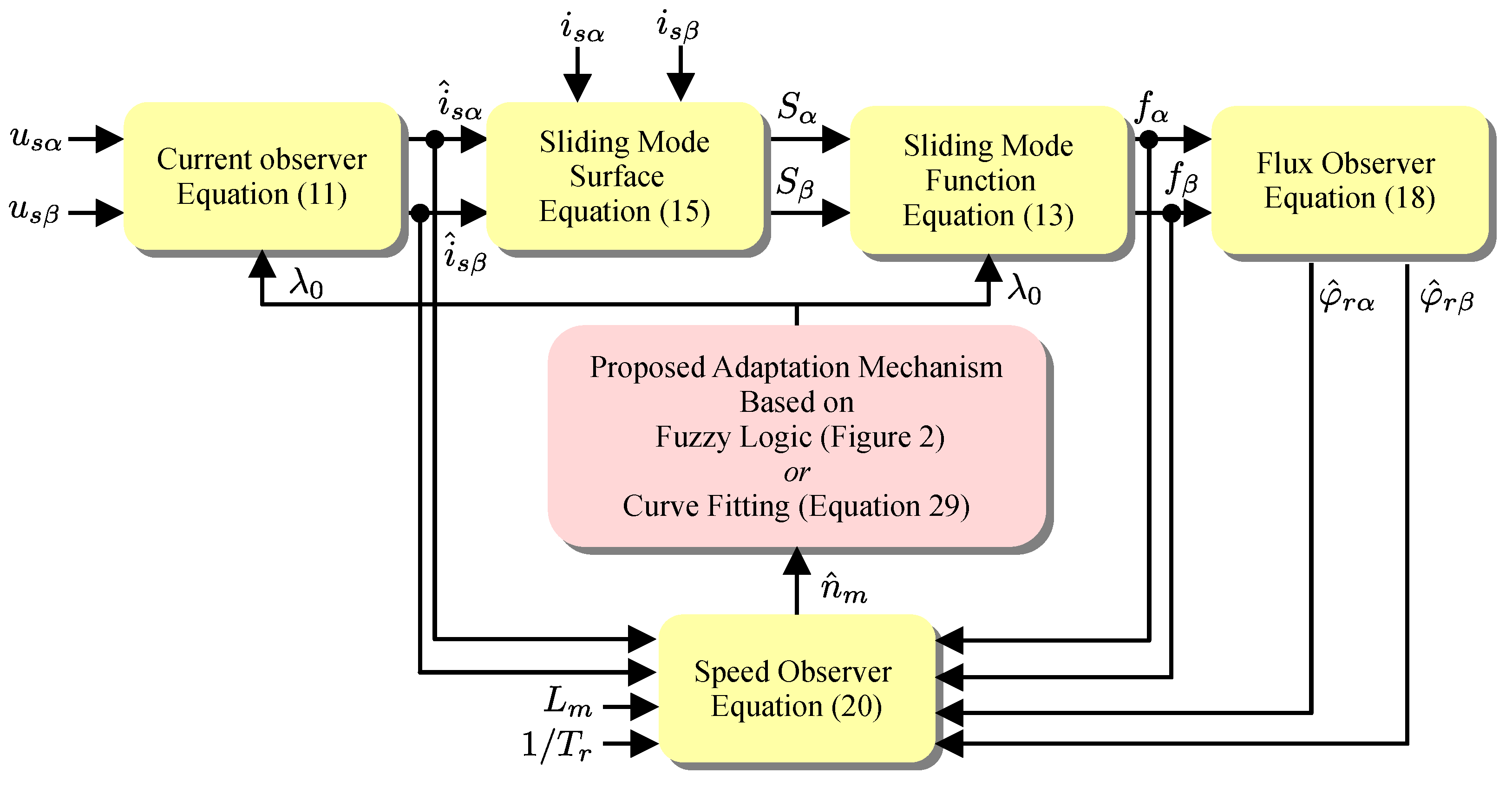
In this subsection, the proposed FA-SMO method, using fuzzy logic to perform the λ 0 changes between the predetermined limits according to the operation speed of IM, is introduced. To realize the proposed FA-SMO method, the n ^ m (estimated rotor mechanical speed) feedback is needed to obtain the proper λ 0 value. The block diagram for the proposed FA-SMO is shown in Figure 1. Furthermore, the fuzzy logic-based adaptation mechanism used in the proposed FA-SMO is shown in Figure 2. In Figure 1 and Figure 2, “ . ^ ” refers to the estimated state or parameter.
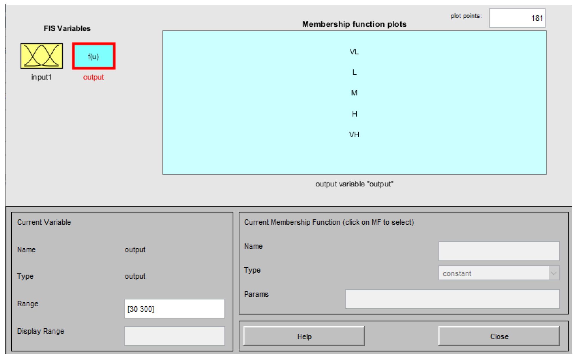
Since the adaptive neuro-fuzzy inference system (ANFIS) tool of Matlab is utilized in the design process of FA-SMO, the defuzzification phase is carried out by using the wtaver method based on the Sugeno inference method in Figure 2. In addition, during the training phase of the ANFIS block, the selected λ 0 values obtained through experimental experience are used as training data. The hybrid training method in the MATLAB 2024 ANFIS block is employed, which automatically determines the membership functions, as shown in Figure 3 and Figure 4. Figure 5 presents the ANFIS model structure, while Figure 6 illustrates the fuzzy surface view between λ 0 and n m . As a result of the training, a training error of 3.27 occurred. Here, the n m value selected as input of the fuzzy system which has the following membership functions of very low (VL), low (L), medium (M), high (H), and very high (VH). By defining five membership functions, λ 0 changes are performed where λ 0 should be significantly changed according to the speed variation. To not significantly increase the computational load of FA-SMO, five membership functions resulting in low training error are chosen. In addition, Gaussian-shaped membership functions were preferred for the lowest training error. Five rules used in the proposed FA-SMO are given in Table 1.

3.2. Curve Fitting Adaptive SMO

In this subsection, the curve fitting method is used to change λ 0 in the proposed CFA-SMO method given in Figure 1 to increase the estimation performance of C-SMO. Since the proper λ 0 values are determined in real-time experiments, it is noticed that it is possible to perform the λ 0 changes based on rotor speed by using a first-order function of n m . Thus, using a simple function as in [36,38,41], λ 0 adaptation is achieved while preserving the computational efficiency of C-SMO, as in the FA-SMO method. The first-order function to be used for this purpose is determined using the Matlab Curve Fitting Toolbox as follows.
λ 0 = 0.2678 | n m | + 33.66
As can be seen from (28), similar to the FA-SMO method, n m feedback is required to calculate the proper λ 0 values in the CFA-SMO method. Thus, by using (28) in the λ 0 adaptation of CFA-SMO, it is possible to obtain a proper λ 0 value according to the operation speed of IM. Since both FA-SMO and CFA-SMO methods utilize experimentally determined λ 0 values, they present similar λ 0 values for the same operation speed of IM. Thus, the similar λ 0 values lead to similar performance for the proposed A-SMO methods in this paper.

4. Experimental Results

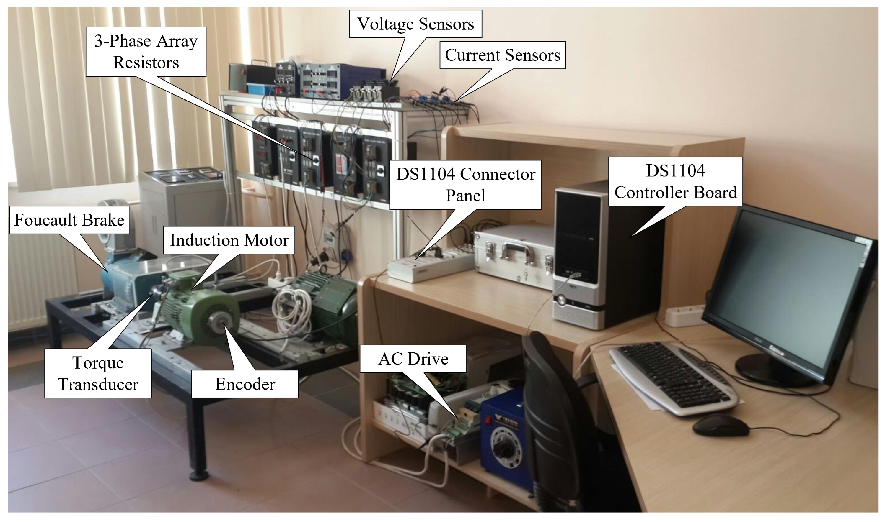
To test the proposed A-SMOs and demonstrate their superiority over C-SMO, they are tested in real-time experiments including a wide range of speeds with and without load variations. The experimental setup used in these tests is given in Figure 7, and its block diagram representation is illustrated in Figure 8. Here, a 30 N·m Foucault brake is used to load the three-phase squirrel-cage IM parameters which are presented in Table 2. To perform i s α β and u s α β measurements, LA55-P/SP1 and LV 100–400 transducers are used, respectively. Moreover, ω m and t L are measured by using an encoder with 5000 lines/rev and a 50 N·m torque transducer, respectively. As seen in Figure 8, the ω m and t L measurements are not utilized in the proposed A-SMOs and the C-SMO methods. The ω m is measured only to validate the ω m estimated by the proposed and conventional observers. Additionally, the t L measurement is carried out to monitor the load condition under which IM operates. Furthermore, a three-phase array resistor is employed to externally add resistances in series R s with the stator windings of the IM in order to investigate the effect of variations on the proposed A-SMOs and C-SMO. As shown in Figure 8, to ensure a fair comparison between the proposed A-SMOs and C-SMO, all observers are operated and tested under open-loop conditions, and an AC drive is utilized to drive the IM with pulse-width modulated voltages and currents as in [5]. The proposed A-SMOs and the C-SMO methods were designed in the Matlab S-function block, using C/C++ language, and implemented on the DS1104 controller board. For online visualization of the data in real-time experiments, the dSPACE ControlDesk interface software is used. Utilizing the data-saving feature of ControlDesk, all data presented in this paper are saved and then plotted by using Matlab to provide high-quality figure presentations. Here, the sampling time (T) is 100 μ s for all tests. Also, as in [13], proposed A-SMOs are operated simultaneously and separately from the AC drive with utilization of i s α β and u s α β applied to IM, and the AC drive also runs in open-loop.
By utilizing the experimental setup in Figure 7 and Figure 8, the proposed A-SMOs are tested under challenging scenarios including usage of measured and estimated current, zero speed operation, load variations, and parameter changes ( R s changes). In the real-time implementation of the proposed FA-SMO, the fuzzy logic controller is converted into a 1D look-up table to reduce the computational load and also the additional computational load caused by the proposed adaptive structures is obtained by measuring the execution time of each algorithm. Furthermore, the proposed A-SMOs are compared to C-SMO in all test scenarios. The details of the test scenarios are presented in the following subsections.

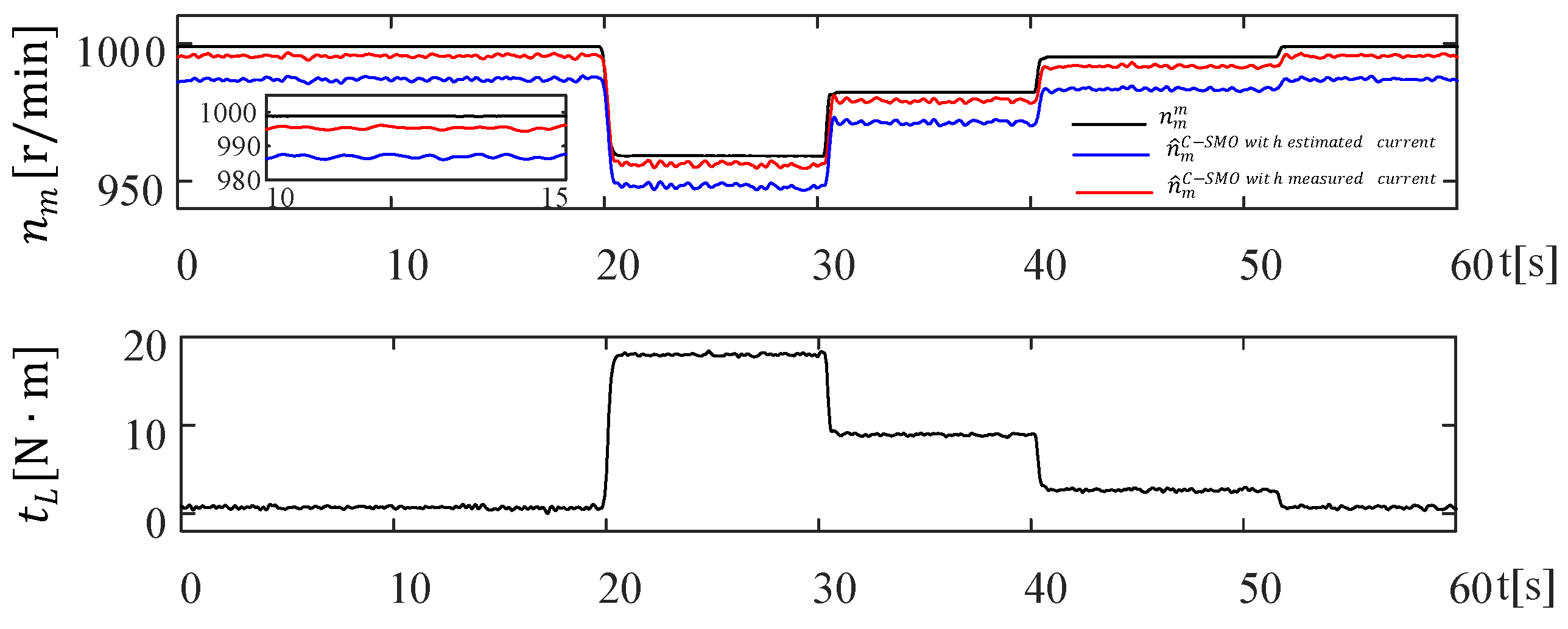
4.1. Scenario I: Usage of Measured Currents and Estimated Currents (Figure 9)

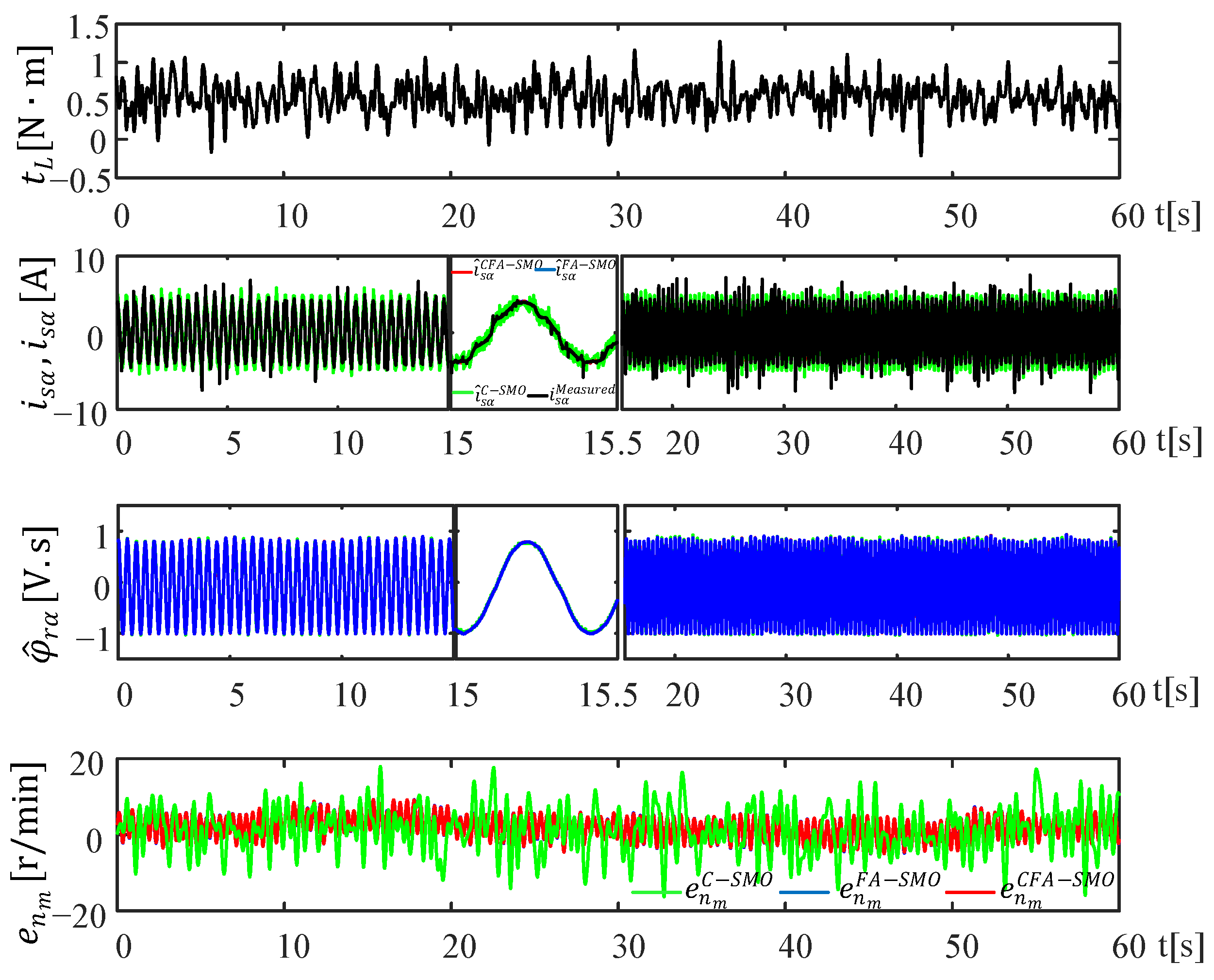
Scenario I tests the estimation performance of the measured stator currents of IM and the estimated currents of SMO in the case of sudden t L variations for the high-speed region. Thus, the aim is to validate the correctness of the measured currents, used in (20) instead of the estimated currents which present chattering free against unknown t L inputs. The obtained results are presented in Figure 9.

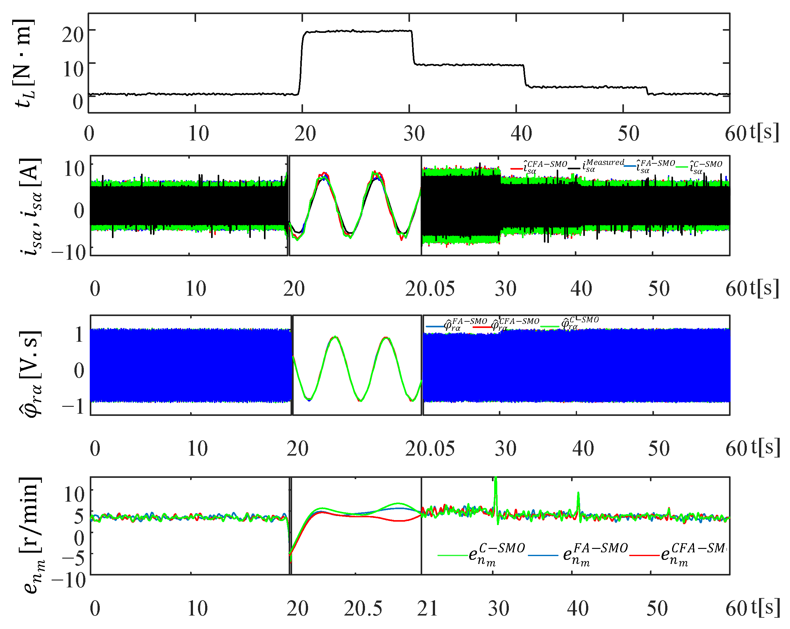
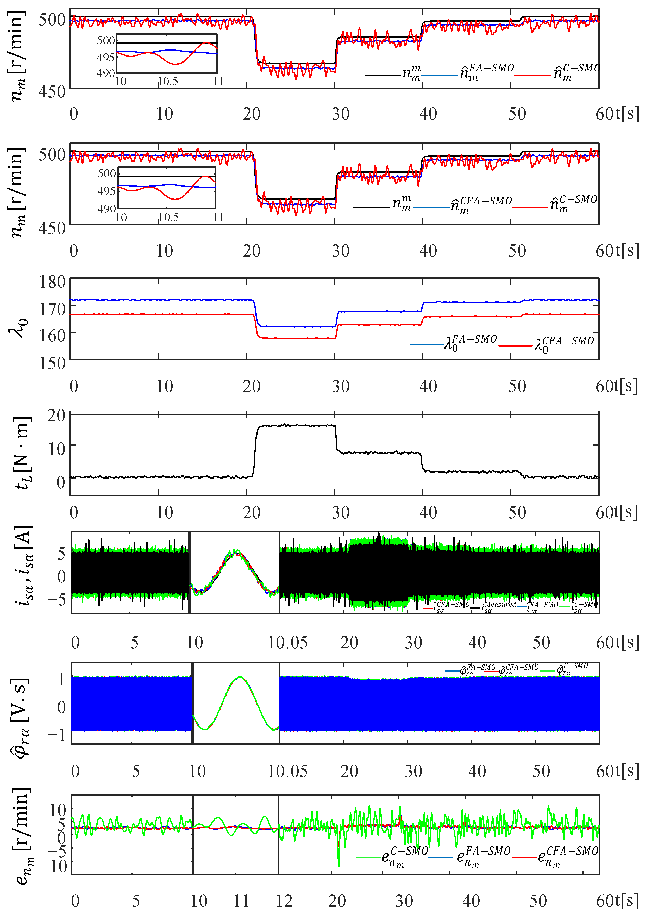
4.2. Scenario II: Load Torque Variation Test (Figure 10, Figure 11 and Figure 12)

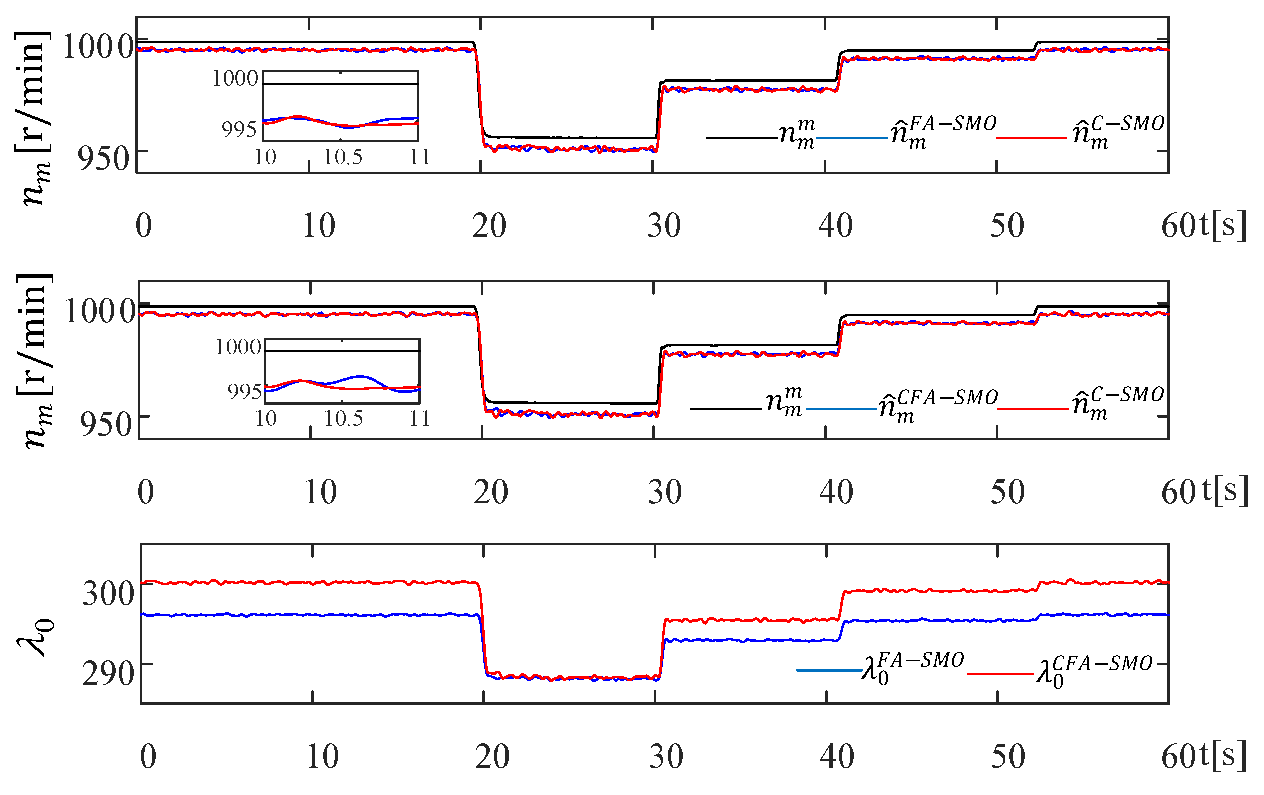
Scenario II tests the estimation performance of the proposed A-SMOs and C-SMO in the case of sudden t L variations for three different speed regions, namely high, medium, and low speeds. Thus, the aim is to validate the robustness of the proposed A-SMOs against unknown t L inputs. The estimation results and corresponding estimation errors are presented in Figure 10, Figure 11 and Figure 12 for high, medium, and low speeds, respectively. In all tests shown in Figure 10, Figure 11 and Figure 12, it is also possible to see the changes of λ 0 in A-SMOs and their favorable effects on ω m estimation by particularly inspecting e n m .

4.3. Scenario III: Speed-Reversal Test (Figure 13)

IM runs at its rated speed at no-load. After a sudden increase in load torque from no-load to rated load at approximately t = 40 s, the speed reversal is repeated at around t = 50 s. In this scenario demonstrated in Figure 13, the performance of the proposed A-SMO observers is intended to be tested in a wide range of speed ranges, including the nominal speed for each rotation direction. Additionally, λ 0 values calculated by A-SMOs and the Lyapunov stability criterion are compared in this scenario.

4.4. Scenario IV: Sensitivity Tests on Parameters (Figure 14, Figure 15 and Figure 16)

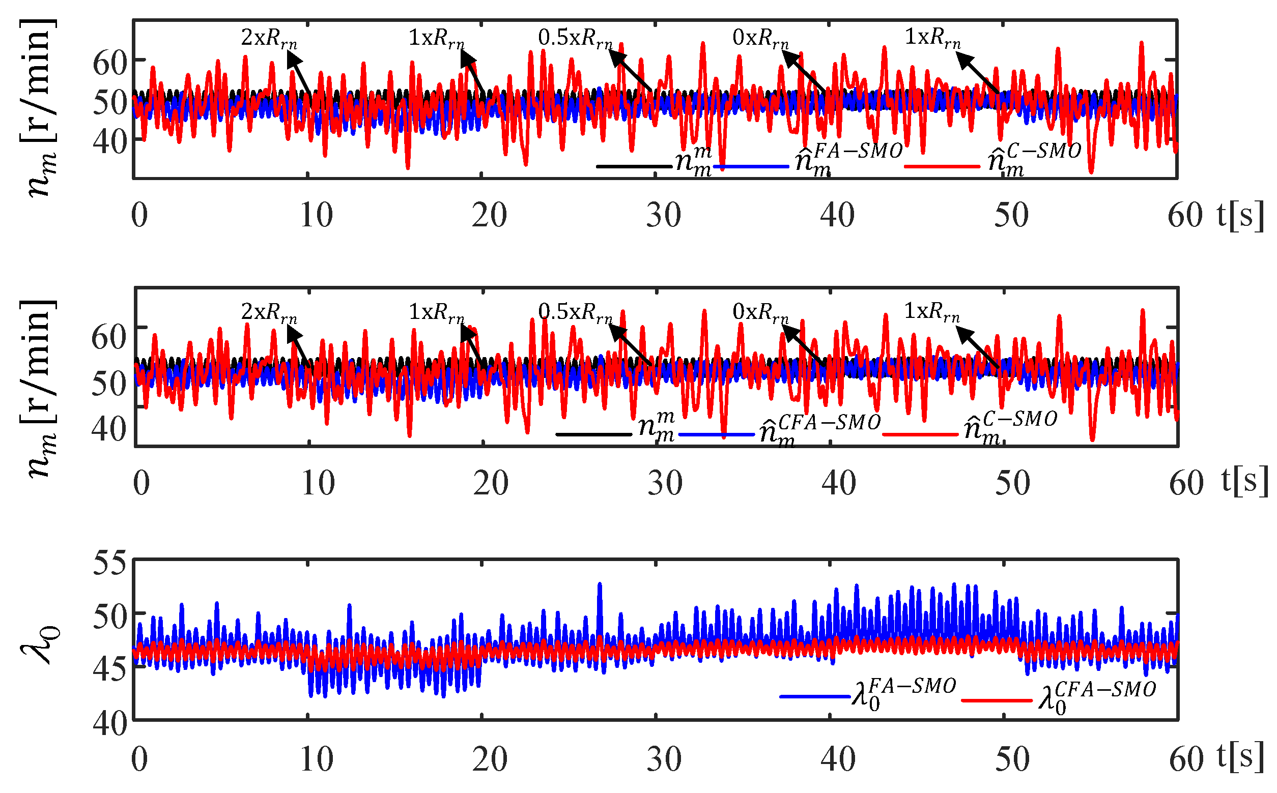
To examine the effects of parameter variations on the proposed A-SMOs, first of all an R s -change test is performed in the low-speed region, where the R s variation is more effective due to the relatively high voltage drop ratio on R s . Later, the R r -change is also examined in the low-speed operation, similar to R s -change while L m -change is performed in the high-speed operation. For this purpose, the R s changes are performed as in Figure 14 through the group resistors connected in series to the stator terminals of IM. Since a squirrel cage IM is used in the experimental setup, it is not possible to change R r by externally adding a group of series resistors. Therefore, to perform R r variations in Figure 15, the applied R r is defined as R r = γ * R r n in the A-SMOs and C-SMO algorithms, and the variations in R r are generated by changing γ from 0 to 2. Similarly, the applied L m is defined as L m = η * L m n in the A-SMOs and C-SMO algorithms, and thus variations in L m at high-speed operation as in Figure 16 are developed by varying η from 0.5 to 2. Here, R r n and L m n are the rated values of R r and L m , respectively. γ and η represent uncertainties related to R r and L m , respectively. Thus, it is possible to compare the performance of the proposed A-SMOs with C-SMO under parameter variations.

4.5. Scenario V: Continuous Zero Speed Test (Figure 17)

To test the estimation performance of the proposed A-SMOs in the case of continuous zero speed operation, the IM speed is decreased to zero while it is operating in the low-speed region without load as shown in Figure 17. The results confirm that the estimation performance of the proposed observers is still satisfactory and the estimations do not diverge despite the fact that IM is continuously operating at zero speed.
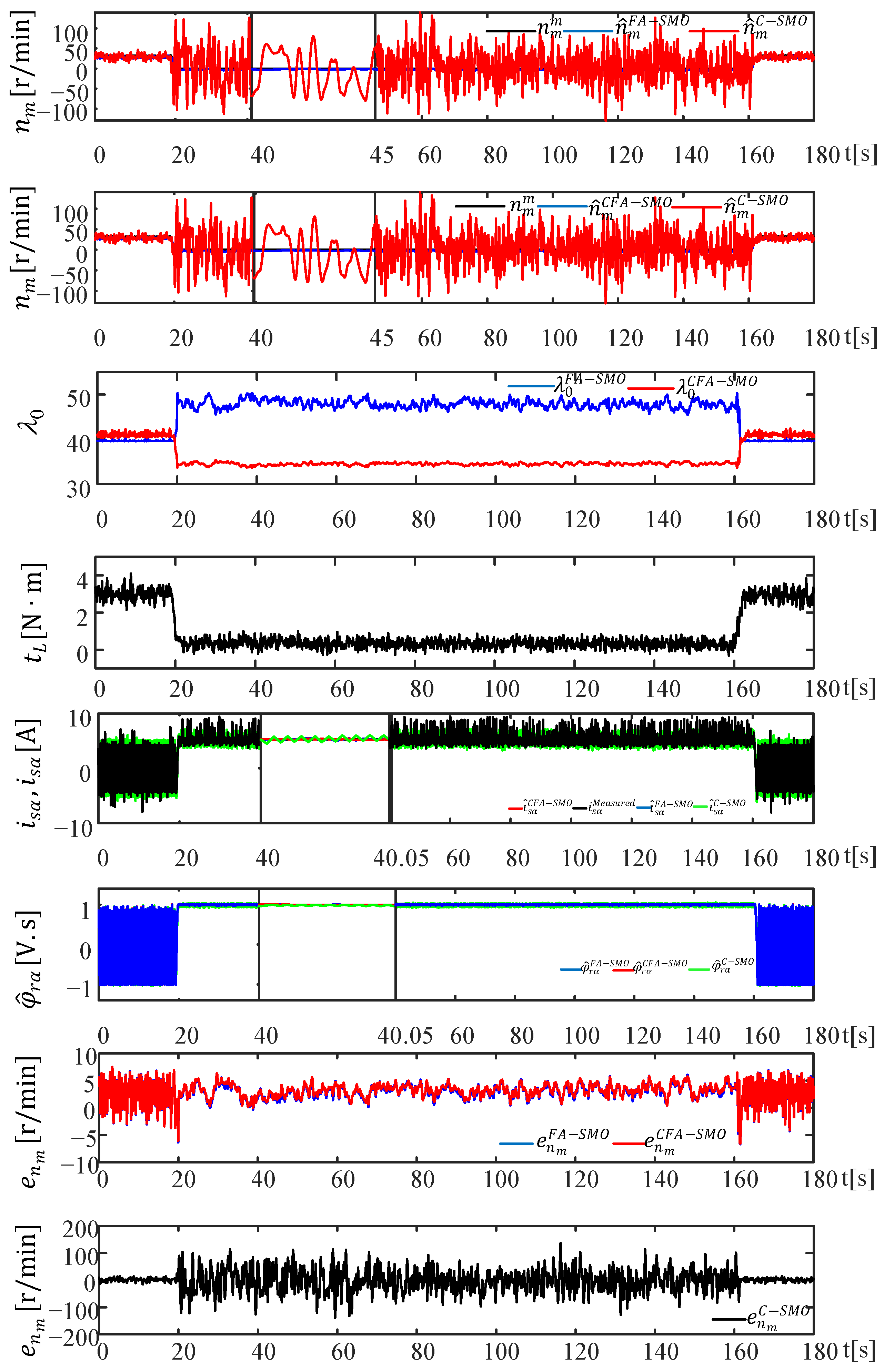
Finally, the resulting mean square error (MSE), root mean square error (RMSE), and integral absolute error (IAE) values for estimations associated with each scenario are presented in Table 3, Table 4 and Table 5, respectively. The total harmonic distortion (THD) of the estimated α -axis current for the proposed A-SMOs and C-SMO is given in Table 6. The execution times for each observer obtained by calculating the average value for each iteration are given in Table 7. When the real-time test results given in Figure 9, Figure 10, Figure 11, Figure 12, Figure 13, Figure 14, Figure 15, Figure 16 and Figure 17 are examined, the following observations can be made:
  • To show the effect of the measured currents usage in the ω m estimation in (20), the ω m -estimation results are also presented in Figure 9 for both using measured and estimated currents cases. It is clear that the ω m estimation can be improved by using measured currents, which is the main reason why the measured currents are used in (20) in this paper.
  • The best value of λ 0 is determined for high-speed operation of IM in C-SMO and is kept constant in C-SMO for all scenarios. That is why the performance of C-SMO and the proposed A-SMOs are close to each other in Figure 10. As can be seen from Figure 11 and Figure 12, while the IM speed is decreasing from the high-speed region to the medium- or low-speed region, the constant λ 0 in C-SMO leads to chattering in the estimations. On the other hand, the proposed A-SMO methods can overcome this challenge by adjusting λ 0 to its predetermined proper value. The obtained MSE, RMSE, and IAE results demonstrate that the proposed A-SMO methods outperform C-SMO for all presented results. Furthermore, the THD values calculated for 1000 (r/min), 500 (r/min), and 50 (r/min) with/without load condition in Table 6 also highlight the superior performance of FA-SMO and CFA-SMO over C-SMO.
  • In the speed-reversal scenario, it can be seen in Figure 13 that the proposed A-SMOs are superior to C-SMOs, especially in the low-speed region. Moreover, it has been proven that the proposed A-SMOs satisfy the Lyapunov stability condition for each speed region.
  • From the results of the R s and R r variation tests at low speeds in Figure 14 and Figure 15, it is observed that the proposed A-SMOs in this paper demonstrate superiority (i.e., reduced chattering) over C-SMO due to their λ 0 adaptation. This can also be seen from the resulting MSE, RMSE, and IAE values in Table 3, Table 4 and Table 5, which verify the effectiveness of the proposed A-SMOs under R s and R r uncertainties. Moreover, in the L m variation test at high-speed operation (Figure 16), both the proposed A-SMOs and C-SMO exhibit similar estimation performance, since they have approximately the same λ 0 values. Furthermore, these challenging L m changes do not have a significant impact on their estimation performance, demonstrating the robustness of SMO methods against L m variations for both the proposed A-SMOs and C-SMO.
  • In continuous zero speed operation tests, it is obvious that the estimation performances of the proposed methods are satisfactory and the proposed methods easily overcome this challenge while C-SMO has high values chattering in the estimated ω m .
  • The proposed A-SMO methods (FA-SMO and CFA-SMO) are designed to preserve the low-computational-load superiority of C-SMO. As can be seen in Table 7, compared to C-SMO, the proposed FA-SMO and CFA-SMO methods resulted in a slight increase in computational load of only 0.55 μ s and 0.5 μ s, respectively.
  • The proposed A-SMOs are built upon the C-SMO structure; therefore, the slight increase in their computational load mainly results from the λ 0 adaptation mechanisms. In addition, to further evaluate and compare the computational efficiency of the proposed A-SMOs, the computational complexities of the sliding mode function of (13) utilized in both C-SMO and A-SMOs and the one used in STSMO (Equation (16) in Nurettin and Inanc [9]) are presented in Table 8, as calculated by Bonaldo et al. [47]. The results indicate that both C-SMO and the proposed A-SMOs exhibit lower computational complexity in their sliding mode functions compared to STSMO in Nurettin and Inanc [9]. Moreover, when the proposed adaptive mechanisms in (29) are considered alongside the adaptive mechanism (Equation (23) in Nurettin and Inanc [9]), a similar analysis as in Table 8 can be realized. Since the adaptive mechanism in Nurettin and Inanc [9] involves multiple addition, division, multiplication, and absolute value operations, its estimated computational cost is higher than those of the simpler adaptive structures proposed in this paper. These results are also coherent with the past results presented in Ullah et al. [48], which compares the conventional and super twisting sliding mode controllers.

5. Conclusions

In this paper, two novel A-SMOs using only the stator current errors in sliding surface are proposed for the speed sensorless IM drives utilized in both EV and industrial applications. By adjusting the λ 0 value in A-SMO methods, the aim is to overcome the operation region-based performance deteriorations of C-SMO. The adaptation of λ 0 through fuzzy logic and curve-fitting methods enhances estimation performance without significantly increasing the computational load.
The proposed A-SMOs estimate i s α , i s β , φ r α , φ r β , and ω m in real time, utilizing measured currents and voltages. Experimental results demonstrate that A-SMOs outperform C-SMO in terms of estimation accuracy, robustness against variations in R s , R r , and L m , and reduced chattering, particularly at low speeds. At higher speeds, proposed methods achieve similar estimation performance to C-SMO under L m variations, although they still require accurate values of R s and R r for optimal performance.
Despite these improvements, limitations remain. The proposed methods rely on precise rotor and stator parameters for high-speed operation, and their performance may degrade under extreme operating conditions or parameter uncertainties. Future work will focus on addressing these limitations, including adaptive techniques to handle parameter variations and further reduction of computational complexity.
Finally, the proposed A-SMOs, featuring lower computational load and adaptive mechanisms independent of IM model parameters, outperform previous studies such as [9,39], making them more feasible for real-time sensorless control of IMs in both EV and industrial applications.

Author Contributions

Conceptualization, H.B.D. and M.B.; Methodology, H.B.D. and M.B.; Software, H.B.D. and R.Y.; Validation, H.B.D., R.Y. and E.Z.; Formal Analysis, H.B.D., M.B. and R.Y.; Investigation, H.B.D., M.B., R.Y. and E.Z.; Data Curation, H.B.D.; Writing—Original Draft Preparation, H.B.D., M.B., R.Y. and E.Z.; Writing—Review & Editing, H.B.D., M.B., R.Y. and E.Z.; Visualization, H.B.D., R.Y. and E.Z.; Supervision, M.B. All authors have read and agreed to the published version of the manuscript.

Funding

This research received no external funding.

Data Availability Statement

The data presented in this study are available on request from the corresponding author.

Conflicts of Interest

The authors declare no conflicts of interest.

References

  1. Holtz, J. Sensorless control of induction motor drives. Proc. IEEE 2002, 90, 1359–1394. [Google Scholar] [CrossRef]
  2. Demir, R.; Barut, M. Novel hybrid estimator based on model reference adaptive system and extended Kalman filter for speed-sensorless induction motor control. Trans. Inst. Meas. Control 2018, 40, 3884–3898. [Google Scholar] [CrossRef]
  3. Zaky, M.S.; Metwaly, M.K. Improved MRAS observer with rotor flux correction terms and FLC-based adaptive law for sensorless induction motor drives. Sci. Rep. 2025, 15, 14769. [Google Scholar] [CrossRef]
  4. Feng, F.; Yang, J.; Hu, H.; Liang, J.; Yu, S. Speed-sensorless model predictive thrust control of linear induction motor based on improved extended Kalman filter observer. Trans. Inst. Meas. Control 2025. [Google Scholar] [CrossRef]
  5. Yildiz, R.; Barut, M.; Zerdali, E. A Comprehensive Comparison of Extended and Unscented Kalman Filters for Speed-Sensorless Control Applications of Induction Motors. IEEE Trans. Ind. Inform. 2020, 16, 6423–6432. [Google Scholar] [CrossRef]
  6. Jouili, M.; Jarray, K.; Koubaa, Y.; Boussak, M. Luenberger state observer for speed sensorless ISFOC induction motor drives. Electr. Power Syst. Res. 2012, 89, 139–147. [Google Scholar] [CrossRef]
  7. Du, T.; Brdys, M. Shaft speed, load torque and rotor flux estimation of induction motor drive using an extended Luenberger observer. In Proceedings of the 1993 Sixth International Conference on Electrical Machines and Drives (Conf. Publ. No. 376), Oxford, UK, 8–10 September 1993; pp. 179–184. [Google Scholar]
  8. Zhang, Y.; Yin, Z.; Zhang, Y.; Liu, J.; Tong, X. A Novel Sliding Mode Observer with Optimized Constant Rate Reaching Law for Sensorless Control of Induction Motor. IEEE Trans. Ind. Electron. 2020, 67, 5867–5878. [Google Scholar] [CrossRef]
  9. Nurettin, A.; İnanç, N. Sensorless Vector Control for Induction Motor Drive at Very Low and Zero Speeds Based on an Adaptive-Gain Super-Twisting Sliding Mode Observer. IEEE J. Emerg. Sel. Top. Power Electron. 2023, 11, 4332–4339. [Google Scholar] [CrossRef]
  10. Zerdali, E.; Menguc, E.C. Novel Complex-Valued Stator Current-Based MRAS Estimators with Different Adaptation Mechanisms. IEEE Trans. Instrum. Meas. 2019, 68, 3793–3795. [Google Scholar] [CrossRef]
  11. Kivanc, O.C.; Ozturk, S.B. Sensorless PMSM Drive Based on Stator Feedforward Voltage Estimation Improved with MRAS Multiparameter Estimation. IEEE/ASME Trans. Mechatronics 2018, 23, 1326–1337. [Google Scholar] [CrossRef]
  12. Zhang, Y.; Zhao, Z.; Lu, T.; Yuan, L.; Xu, W.; Zhu, J. A comparative study of Luenberger observer, sliding mode observer and extended Kalman filter for sensorless vector control of induction motor drives. In Proceedings of the 2009 IEEE Energy Conversion Congress and Exposition, San Jose, CA, USA, 20–24 September 2009; pp. 2466–2473. [Google Scholar] [CrossRef]
  13. Zerdali, E.; Barut, M. The Comparisons of Optimized Extended Kalman Filters for Speed-Sensorless Control of Induction Motors. IEEE Trans. Ind. Electron. 2017, 64, 4340–4351. [Google Scholar] [CrossRef]
  14. Saihi, L.; Boutera, A. Robust sensorless sliding mode control of PMSM with MRAS and Luenberger extended observer. In Proceedings of the 2016 8th International Conference on Modelling, Identification and Control (ICMIC), Algiers, Algeria, 15–17 November 2016; pp. 174–179. [Google Scholar] [CrossRef]
  15. Utkin, V.; Jin, C.; Yan, Z. Sensorless sliding-mode control of induction motors. IEEE Trans. Ind. Electron. 2000, 47, 1286–1297. [Google Scholar] [CrossRef]
  16. Hadj Saïd, S.; M’Sahli, F.; Mimouni, M.; Farza, M. Adaptive high gain observer based output feedback predictive controller for induction motors. Comput. Electr. Eng. 2013, 39, 151–163. [Google Scholar] [CrossRef]
  17. Pudari, M.; Arya, S.R.; Arya, R.K. An improved Sliding Mode Observer for parameter estimation in induction motor drive with optimised gains. Aust. J. Electr. Electron. Eng. 2023, 20, 235–250. [Google Scholar] [CrossRef]
  18. V, K.; Singh, B. Sensorless Control of Induction Motor using MSTOGI based Super Twisting Sliding Mode Flux Observer for Electric Vehicle. In Proceedings of the 2022 IEEE Global Conference on Computing, Power and Communication Technologies (GlobConPT), New Delhi, India, 23–25 September 2022; pp. 1–6. [Google Scholar] [CrossRef]
  19. Sun, Y.; Yang, Z.; Sun, X.; Sun, C. Speed sensorless control of a BL-IM based on an adaptive nonsingular terminal sliding mode observer. Int. J. Electron. 2023, 110, 341–359. [Google Scholar] [CrossRef]
  20. Wang, H.; Ge, X.; Liu, Y.C. Second-Order Sliding-Mode MRAS Observer-Based Sensorless Vector Control of Linear Induction Motor Drives for Medium-Low Speed Maglev Applications. IEEE Trans. Ind. Electron. 2018, 65, 9938–9952. [Google Scholar] [CrossRef]
  21. Mezouar, A.; Fellah, M.; Hadjeri, S. Adaptive sliding-mode-observer for sensorless induction motor drive using two-time-scale approach. Simul. Model. Pract. Theory 2008, 16, 1323–1336. [Google Scholar] [CrossRef]
  22. Zaky, M.; Khater, M.; Shokralla, S.; Yasin, H. Wide-Speed-Range Estimation with Online Parameter Identification Schemes of Sensorless Induction Motor Drives. IEEE Trans. Ind. Electron. 2009, 56, 1699–1707. [Google Scholar] [CrossRef]
  23. Shen, Z.; Yang, Z.; Sun, X.; Pan, W. Sensorless control of bearingless induction motor based on fuzzy dual sliding mode MRAS. Electr. Eng. 2024, 107, 5737–5747. [Google Scholar] [CrossRef]
  24. Rehman, H.; Derdiyok, A.; Guven, M.; Xu, L. A new current model flux observer for wide speed range sensorless control of an induction machine. IEEE Trans. Power Electron. 2002, 17, 1041–1048. [Google Scholar] [CrossRef]
  25. Wang, T.; Wang, B.; Yu, Y.; Xu, D. Discrete Sliding-Mode-Based MRAS for Speed-Sensorless Induction Motor Drives in the High-Speed Range. IEEE Trans. Power Electron. 2023, 38, 5777–5790. [Google Scholar] [CrossRef]
  26. Su, Y.; Yang, Z.; Sun, X.; Pan, W. Speed sensorless control of a bearingless induction motor based on sliding mode observer with improved double power reaching law. Int. J. Electron. 2025, 1–17. [Google Scholar] [CrossRef]
  27. Prince; Yoon, B. Super Twisted Sliding Mode Observer for Enhancing Ventilation Drive Performance. Appl. Sci. 2025, 15, 4927. [Google Scholar] [CrossRef]
  28. Ammar, A.; Belaroussi, O.; Benakcha, M.; Zemmit, A.; Ameid, T. Super-Twisting MRAS Observer-Based Non-linear Direct Flux and Torque Control for Induction Motor Drives. Power Electron. Drives 2024, 9, 374–396. [Google Scholar] [CrossRef]
  29. Zhang, L.; Obeid, H.; Laghrouche, S.; Hamerlain, M. Adaptive High Order Sliding Mode Observer of Linear Induction Motor. In Proceedings of the 2018 15th International Workshop on Variable Structure Systems (VSS), Graz, Austria, 9–11 July 2018; pp. 96–101. [Google Scholar] [CrossRef]
  30. Gonzalez, T.; Moreno, J.A.; Fridman, L. Variable Gain Super-Twisting Sliding Mode Control. IEEE Trans. Autom. Control 2012, 57, 2100–2105. [Google Scholar] [CrossRef]
  31. Kandoussi, Z.; Boulghasoul, Z.; Elbacha, A.; Tajer, A. Fuzzy sliding mode observer based sensorless Indirect FOC for IM drives. In Proceedings of the 2015 Third World Conference on Complex Systems (WCCS), Marrakech, Morocco, 23–25 November 2015; pp. 1–6. [Google Scholar] [CrossRef]
  32. Rao, S.; Buss, M.; Utkin, V. An adaptive sliding mode observer for induction machines. In Proceedings of the 2008 American Control Conference, Seattle, WA, USA, 11–13 June 2008; pp. 1947–1951. [Google Scholar] [CrossRef]
  33. Xu, W.; Qu, S.; Zhao, L.; Zhang, H. An Improved Adaptive Sliding Mode Observer for Middle- and High-Speed Rotor Tracking. IEEE Trans. Power Electron. 2021, 36, 1043–1053. [Google Scholar] [CrossRef]
  34. Parasiliti, F.; Petrella, R.; Tursini, M. Adaptive sliding mode observer for speed sensorless control of induction motors. In Proceedings of the Conference Record of the 1999 IEEE Industry Applications Conference, Thirty-Forth IAS Annual Meeting (Cat. No.99CH36370), Phoenix, AZ, USA, 3–7 October 1999; Volume 4, pp. 2277–2283. [Google Scholar] [CrossRef]
  35. Tursini, M.; Petrella, R.; Parasiliti, F. Adaptive sliding-mode observer for speed-sensorless control of induction motors. IEEE Trans. Ind. Appl. 2000, 36, 1380–1387. [Google Scholar] [CrossRef]
  36. Keyhani, A.; Bogdan Proca, A.; Miller, J. Sensorless control of induction motors. In Proceedings of the IEMDC 2001, IEEE International Electric Machines and Drives Conference (Cat. No.01EX485), Cambridge, MA, USA, 17–20 June 2001; pp. 337–344. [Google Scholar] [CrossRef]
  37. Kim, S.M.; Han, W.Y.; Kim, S.J. Design of a new adaptive sliding mode observer for sensorless induction motor drive. Electr. Power Syst. Res. 2004, 70, 16–22. [Google Scholar] [CrossRef]
  38. Tarchala, G.; Orlowska-Kowalska, T. Sliding Mode Speed Observer for the Induction Motor Drive with Different Sign Function Approximation Forms and Gain Adaptation. Prz. Elektrotechniczny 2013, 1, 13. [Google Scholar]
  39. Hu, Z.; Gao, C.; Guan, H.; Xiong, J.; Zhang, K. Speed Sensorless Model Predictive Flux Control of Induction Motor Based on Adaptive Gain Sliding Mode Observer. In Proceedings of the 2020 IEEE 1st China International Youth Conference on Electrical Engineering (CIYCEE), Wuhan, China, 1–4 November 2020; pp. 1–7. [Google Scholar] [CrossRef]
  40. Bai, W.; Cai, J.; Kuang, Y.; Wang, Y.; Hua, X.; Ma, Z. Research on a novel adaptive sliding mode observer sensorless control for dual three-phase permanent magnet synchronous motors. Results Eng. 2025, 27, 105709. [Google Scholar] [CrossRef]
  41. Wang, T.; Wang, B.; Yu, Y.; Xu, D. High-Order Sliding-Mode Observer with Adaptive Gain for Sensorless Induction Motor Drives in the Wide-Speed Range. IEEE Trans. Ind. Electron. 2023, 70, 11055–11066. [Google Scholar] [CrossRef]
  42. Zerzeri, M.; Moussa, I.; Khedher, A. Adaptive Sliding-Mode Observer for FOC of IM Drives Fed by Soft-VSI Topology: Wind Turbine Emulator Application. In Proceedings of the 2024 IEEE International Conference on Advanced Systems and Emergent Technologies (IC_ASET), Hammamet, Tunisia, 27–29 April 2024; pp. 1–6. [Google Scholar] [CrossRef]
  43. Bu, W.; Tao, W.; Chen, Y. Research on Sliding Mode Variable Structure Model Reference Adaptive System Speed Identification of Bearingless Induction Motor. Energies 2024, 17, 2615. [Google Scholar] [CrossRef]
  44. Shi, L.; Lv, M.; Li, P. Sensorless Position Control in High-Speed Domain of PMSM Based on Improved Adaptive Sliding Mode Observer. Processes 2024, 12, 2581. [Google Scholar] [CrossRef]
  45. Hu, J.; Wu, B. New integration algorithms for estimating motor flux over a wide speed range. IEEE Trans. Power Electron. 1998, 13, 969–977. [Google Scholar] [CrossRef]
  46. Demir, H.B.; Barut, M.; Yildiz, R. The Effect of Measured Current Usage in Conventional Sliding Mode Observer Over Induction Motor Speed Estimation. In Proceedings of the VI, International Turkic World Congress on Science and Engineering (TURK-COSE 2024), TURK-COSE, Baku, Azerbaijan, 19–21 December 2024; pp. 7.56–7.64. [Google Scholar]
  47. Bonaldo, J.; Riccio, J.; Zerdali, E.; Rivera, M.; Monteiro, R.; Wheeler, P. Comparative Analysis of Weighting-Factor-Free Predictive Control Strategies for Direct Torque Control in Permanent Magnet Synchronous Machines. Processes 2025, 13, 2614. [Google Scholar] [CrossRef]
  48. Ullah, A.; Ullah, S.; Zhang, Z.; Jianfei, P. Smooth super-twisting sliding mode control design with high order super-twisting observer for speed tracking control of permanent magnet synchronous motor drive system. ISA Trans. 2025, 162, 227–242. [Google Scholar] [CrossRef] [PubMed]
Figure 1. The block diagram of the proposed FA-SMO and CFA-SMO methods.
Energies 18 05530 g001
Figure 2. The fuzzy logic-based adaptation mechanism in the proposed FA-SMO.
Energies 18 05530 g002
Figure 3. Fuzzy logic block input membership functions of FA-SMO.
Energies 18 05530 g003
Figure 4. Fuzzy logic block output membership functions of FA-SMO.
Energies 18 05530 g004
Figure 5. ANFIS model structure of FA-SMO.
Energies 18 05530 g005
Figure 6. Fuzzy surface view ( n m - λ 0 ).
Energies 18 05530 g006
Figure 7. The experimental setup used in this paper.
Energies 18 05530 g007
Figure 8. Block diagram of the experimental setup in Figure 7.
Energies 18 05530 g008
Figure 9. Test results against usage of the measured and estimated currents in the ω m estimation.
Energies 18 05530 g009
Figure 10. Real-time estimation results for steps like t L changes in the high-speed region.
Energies 18 05530 g010aEnergies 18 05530 g010b
Figure 11. Real-time estimation results for steps like t L changes in the medium-speed region.
Energies 18 05530 g011
Figure 12. Real-time estimation results for steps like t L changes in the low-speed region.
Energies 18 05530 g012
Figure 13. Estimation results for speed reversal with and without load conditions in the high-speed region.
Energies 18 05530 g013
Figure 14. Estimation results for R s changes in the low-speed operation region.
Energies 18 05530 g014
Figure 15. Estimation results for R r changes in the low-speed operation region.
Energies 18 05530 g015aEnergies 18 05530 g015b
Figure 16. Estimation results for L m changes in the high-speed operation region.
Energies 18 05530 g016
Figure 17. Estimation results with and without load conditions in the zero speed region.
Energies 18 05530 g017
Table 1. Rules used in the proposed FA-SMO.
Input Membership FunctionsVLLMHVH
Output Membership FunctionsVLLMHVH
Table 2. The rated values and parameters of the three-phase IM used in experiments.
ParameterValueParameterValue
P 2.2 kW R s 3.03 Ω
V 380 V R r 2.54 Ω
I 5.5 A L s 0.1466 H
f 50 Hz L r 0.1524 H
N m 950 r / min L m 0.135 H
τ l 22 Nm J t 0.055 kg·m2
p p 3 B t 0.001 Nm / ( rad / s )
Table 3. Resulting MSE values.
MethodUsing Measured CurrentsUsing Estimated Currents
e n m e n m
Figure 912.016135.307
MethodC-SMOFA-SMOCFA-SMO
e i s α e n m e i s α e n m e i s α e n m
Figure 101.07216.2771.10316.5761.07415.771
Figure 110.60519.9480.3968.6270.3938.575
Figure 120.42432.7150.06110.5230.06110.512
Figure 130.84342.2220.76236.2990.74736.261
Figure 140.42865.2980.06261.1300.06160.939
Figure 150.42436.1680.05913.1020.05913.079
Figure 161.00526.8841.09124.1291.07724.393
Figure 170.4181370.10.06611.2600.06312.135
Table 4. Resulting RMSE values.
MethodUsing Measured CurrentsUsing Estimated Currents
e n m e n m
Figure 93.46611.632
MethodC-SMOFA-SMOCFA-SMO
e i s α e n m e i s α e n m e i s α e n m
Figure 101.0354.0341.05014.0711.0363.971
Figure 110.7784.4660.6292.9370.6272.928
Figure 120.6515.7190.2483.2430.2483.242
Figure 130.9186.4970.8736.0240.8646.021
Figure 140.6548.0800.2497.8180.2477.806
Figure 150.6516.0130.2443.6160.2433.616
Figure 161.0025.1851.0444.9121.0384.938
Figure 170.64637.0140.2563.3550.2503.483
Table 5. Resulting IAE values.
MethodUsing Measured CurrentsUsing Estimated Currents
e n m e n m
Figure 92.407 × 1058.272 × 105
MethodC-SMOFA-SMOCFA-SMO
e i s α e n m e i s α e n m e i s α e n m
Figure 106.056 × 1042.788 × 1056.161 × 1042.821 × 1056.0738 × 1042.747 × 105
Figure 114.516 × 1042.711 × 1053.556 × 1042.053 × 1053.549 × 1042.048 × 105
Figure 123.899 × 1043.246 × 1059.279 × 1031.910 × 1059.320 × 1031.909 × 105
Figure 135.142 × 1043.746 × 1054.630 × 1043.618 × 1054.584 × 1043.610 × 105
Figure 143.912 × 1044.601 × 1059.595 × 1034.694 × 1059.478 × 1034.691 × 105
Figure 153.127 × 1042.743 × 1057.443 × 1031.720 × 1057.397 × 1031.717 × 105
Figure 163.887 × 1041.880 × 1054.023 × 1041.786 × 1054.007 × 1041.789 × 105
Figure 173.750 × 1041.874 × 1068.922 × 1032.108 × 1058.065 × 1032.210 × 105
Table 6. Resulting THD values.
MethodC-SMOFA-SMOCFA-SMO
Load ConditionNo-LoadLoadedNo-LoadLoadedNo-LoadLoaded
Figure 1019.6013.0718.4812.5119.3512.31
Figure 1120.2914.4112.898.5312.978.50
Figure 1223.9122.039.948.099.908.15
Table 7. Execution times for each observer.
C-SMOFA-SMOCFA-SMO
1.65  μ s2.20  μ s2.15  μ s
Table 8. Computational cost estimation for sliding mode function used in C-SMO, FA-SMO/CFA-SMO, and STSMO strategies, the considering DS-1104 microprocessor.
C-SMOFA-SMO/CFA-SMOSTSMO
OperationQuantityCyclesQuantityCyclesQuantityCycles
Addition/subtraction----22
Multiplication with constant221144
Multiplication with variable--1313
Comparisons ( sgn )111122
Absolute value----11
Square root----120
Estimated total-3-5-32
Disclaimer/Publisher’s Note: The statements, opinions and data contained in all publications are solely those of the individual author(s) and contributor(s) and not of MDPI and/or the editor(s). MDPI and/or the editor(s) disclaim responsibility for any injury to people or property resulting from any ideas, methods, instructions or products referred to in the content.