Abstract
Repurposing end-of-life hydrocarbon wells for geothermal energy generation offers a cost-effective and sustainable strategy to expand low-carbon energy deployment while utilizing existing infrastructure. Fracture-connected horizontal oil and gas well pairs present a promising configuration for enhancing heat transfer in low-permeability reservoirs. Existing modeling approaches, however, lack the ability to simulate transient heat conduction from rock to fluid in such complex fracture pathways. This work develops a mathematical model that couples time-dependent heat conduction in the reservoir rock with convective heat transport within the fractures. This model enables prediction of heat energy productivity of converted well pairs by accounting for realistic boundary conditions and operational parameters. In applying the model to a representative shale gas field in Louisiana, key factors affecting fluid temperature and thermal power output, including fracture geometry, fluid flow rate, and wellbore insulation, were considered. The results demonstrate the feasibility and sensitivity of converting hydrocarbon wells into geothermal energy production, providing critical insight for optimizing such conversions to support the increased demand for clean, sustainable energy.
1. Introduction
The increasing demand for affordable renewable energy has driven the growing interest in repurposing end-of-life hydrocarbon wells to generate geothermal energy [1]. Whilst conventional geothermal systems require high-permeability formations, converted oil and gas wells can leverage existing well infrastructure to reduce development costs and mitigate drilling risks [2]. Fracture-connected horizontal well pairs offer a promising configuration for extracting geothermal heat from low-permeability formations through enhanced contact between the circulating work fluid and the reservoir rock through fractures.
Although several studies have investigated the feasibility of converting abandoned hydrocarbon wells into geothermal service, these approaches have focused on single wellbores or simplified closed-loop setups [3]. These models often neglect the complex transient heat transfer mechanisms occurring in fracture-connected well pairs, where fluid flows through interconnected fractures between injection and production wells. Accurately predicting the heat energy productivity of such systems requires accounting for time-dependent heat conduction from the rock matrix to the work fluid, as well as convective transport within the fractures [4].
Designing and optimizing geothermal well pairs require thorough knowledge of heat transfer process in systems involving fluid injection wellbores, fluid production wellbore, and fractures connecting the two types of wellbores. Mathematical models for describing the transient heat transfer processes in the injection and production of wellbores were provided in works such as Guo et al. [5]. No analytical model is found in the literature to describe the transient heat transfer from formation rock to the flowing fluid in fractures. Solutions for the transient heat conduction from solid to its surface are available for two special boundary conditions. They are valid for (1) the transient heat flow rate for a constant-temperature boundary at the solid surface and (2) the transient temperature at a constant heat flow rate. These two boundary conditions do not exist in the real world of transient heat transfer around the fracture, because both the temperature at the fracture surface and the heat conduction rate are time-dependent. A more rigorous heat transfer solution is needed to solve the problem.
This study develops and demonstrates a mathematical model intended to simulate transient heat transfer in fracture-connected horizontal well pairs that have been converted from hydrocarbon production wells. The model incorporates rigorous solutions to account for time-dependent boundary conditions in heat conduction from rock to fractures and integrates these with wellbore heat transfer models. By applying the model to a sample shale gas well pair in northwestern Louisiana, this work identifies key factors controlling fluid temperature and thermal power deliverability. The results provide critical insights for designing and optimizing geothermal conversions of end-of-life hydrocarbon wells, supporting broader adoption of this sustainable and cost-effective energy production strategy.
2. Mathematical Model
Figure 1 shows a schematic of a geothermal well converted from a horizontal hydrocarbon well pair. The first well, illustrated on the left-hand side, is a multi-fractured horizontal well with the tubing string removed. The second well, illustrated on the right-hand side, is a horizontal well that has been refractured to intersect the first well. The second well can be completed with an insulated tubing string in its vertical section. The injected work fluid, usually water, flows into the old horizontal wellbore, passes through the hydraulic fractures where it harvests geothermal energy, and returns to the surface via the new horizontal wellbore. The major advantage of using the fractured well pair is its enhanced heat transfer from rock formations to the work fluid.
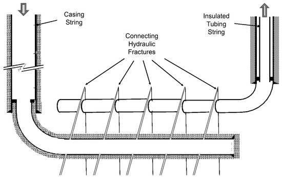
Figure 1.
Schematic of a horizontal well pair converted from end-of-lifetime gas wells.
No method is found in the literature for simulating the heat transfer from the reservoir rock to the fractures in the well systems involving fracture-connected horizontal well pairs. Such a method is developed in this study for predicting the thermal energy productivity of the well pairs. Sensitivity analysis was performed with the model to identify key factors affecting heat transfer efficiency and wells’ thermal energy productivity.
Prediction of thermal energy productivity of a horizontal well pair involves transient heat transfer calculations around the injection wellbore, connecting fractures, and the production wellbore. The transient heat transfer calculations around the injection and production wellbores can be made using the mathematical model described by Guo et al. [5]. The transient heat transfer around a fracture is illustrated in Figure 2. The classic solutions for transient heat conduction from the solid to its flat surface are only valid under two specific conditions: (1) the transient heat flow rate for a constant-temperature boundary at the solid surface, and (2) the transient temperature at a constant heat flow rate. Neither of these two conditions exist in the real world of transient heat transfer around the fracture, because both the temperature at the fracture surface and the heat conduction rate are time-dependent. A more rigorous heat transfer solution is needed to solve the problem.
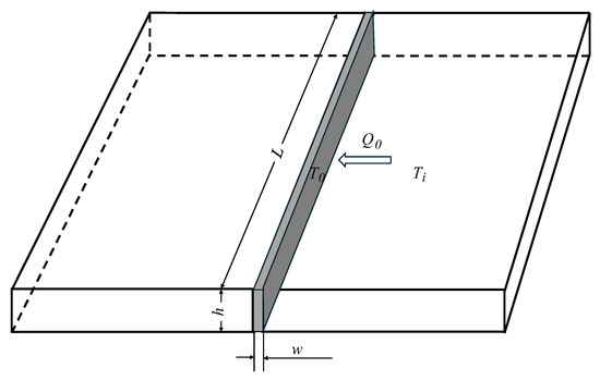
Figure 2.
Transient heat transfer from a rock formation to the fluid in a hydraulic fracture.
As illustrated in Figure 2, the temperature of the fluid in the fracture increases from the entrance to the exit of the fracture. Assuming an average temperature across the fracture length during each cycle of fracture pore volume replacement, the classic heat conduction solution for constant-temperature boundary conditions was coupled with the heat convection inside the fracture. This coupling procedure gives the following equation (derivation is shown in Appendix A):
where Tx is the fluid temperature in °C at the exit of the fracture, K is the thermal conductivity of the rock formation in W/m-C, a is the thermal diffusivity of the rock formation in m2/s, Ti is the initial temperature of the rock formation in °C, T0 is the fluid temperature in °C at the entrance of the fracture, t1 and t2 are the times in s when the fluid enters and leaves the fracture, respectively, during the fracture pore volume replacement, Cp is the specific heat of the fluid in J/kg-°C, r is the fluid density in kg/m3, w is the fracture width (aperture) in m, and is the fracture porosity in the volume fraction.
The following steps were used for computing the time-dependent temperature at the exit of the fracture:
Step 1: Prepare parameter values, including pay zone conditions (surface temperature, geothermal gradient, and depth), rock properties (thermal conductivity and thermal diffusivity), fluid properties (density and specific heat), wellbore properties (dimension and insulation), fracture properties (dimension, permeability, and porosity), and operating conditions (flow rate and temperature of the injection fluid at the top of the injection wellbore).
Step 2: Calculate the temperature of fluid at the bottom of the injection wellbore using the steps described in Guo et al.’s transient heat transfer model [5].
Step 3: Use the calculated fluid temperature at the bottom of the injection wellbore as an input to calculate the fluid temperature at the exit of the fracture with Equation (1). This procedure involves the steps described below.
Calculate the retention time tr of the fluid in the fracture based on the pore volume of the fracture and the fluid flow rate:
where tr is the fluid retention time, L is the fracture length, h is the fracture height, and q is the fluid flow rate.
Initiate loops for fracture pore volume replacement with a time-step size of retention time tr, calculate the fluid temperature at the exit of fracture (Tx) in every time-step using Equation (1), and break the loop at a desired fluid flow time.
Step 4: Use the calculated fluid temperature at the exit of the fracture as an input to calculate the temperature of the fluid at the top of the production wellbore using Guo et al.’s transient heat transfer model [5].
Step 5: Calculate the thermal energy deliverability of the production wellbore based on the calculated fluid temperature at the top of the production wellbore, mass flow rate, and fluid specific heat.
Factor Analysis
A study was conducted for a shale gas field in the Haynesville area, northwestern Louisiana in the United States. Zhang and Guo [4] provided some baseline data, which are summarized in Table 1. The main concerns for well conversion include the following:

Table 1.
Base data for a well in Louisiana in the United States [4].
- 1.
- What is the achievable temperature of the produced fluid?
- 2.
- What is the expected thermal power harvested from the pay zone?
- 3.
- How will the fluid temperature and thermal power decline with time?
- 4.
- What are the factors affecting the temperature of the produced fluid?
- 5.
- How to enhance energy-harvesting efficiency?
Figure 3 shows the model-predicted temperature profile at the end of Year 3 of operation. It is indicated that the injected fluid loses heat to the formation soil at a shallow depth and gains heat at deeper depths due to the geothermal temperature gradient. The injected fluid gains significant heat as it flows through the fracture toward the fluid production wellbore. The temperature of the fluid at the exit of the fracture is 128.8 °C, which is much lower than the geothermal temperature of 170 °C at the deeper depth, meaning that the fluid still has high potential to gain more heat if parameters are optimized. In the production wellbore, the temperature of the fluid first gains heat and then loses heat due to the geothermal gradient. Overall, the fluid temperature declines by 5 °C in the production wellbore and reaches 126.76 °C at the surface. This temperature is adequate for generating electricity with ROC technology [1].
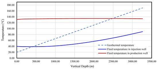
Figure 3.
Geothermal and fluid temperatures in the injection and production wells in relation to depth.
Figure 4 presents the model-predicted transient profiles of temperature and thermal power at the exit of the fracture (bottom of the fluid production wellbore) in the first year of operation. It shows that the temperature, and thus thermal power, of the produced fluid declines quickly in the first 6 months and slowly after 6 months. At the end of the first year, the temperature of the fluid at the exit of the fracture is about 150 °C. This number is slightly higher than the temperature of the fluid at the exit of the fracture of 133 °C at the end of Year 3, indicating a minimal decline in temperature at the fracture exit over the three-year period.
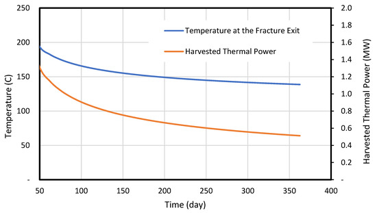
Figure 4.
Model-predicted thermal power and temperature of fluid at fracture exit over time.
Figure 5 presents curves for the model-predicted temperature and thermal power of the produced fluid at varying volumetric flowrates. It shows that the temperature of the produced fluid drops with the flowrate. This is expected, because high-flowrate results in a short retention time of fluid in the fracture and thus a low amount of heat transfer from the formation rock to the fluid in the fracture. The thermal power of the produced fluid increases with the volumetric flowrate, because the thermal power is proportional to the mass flowrate, which increases with the volumetric flowrate.
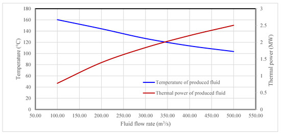
Figure 5.
Effect of fluid volumetric flow rate on the temperature and thermal power of the produced fluid.
Figure 6 indicates that the temperature and thermal power of the produced fluid decline linearly with the thermal conductivity of the insulation layer in the fluid production wellbore. This is expected, because insulation layers with higher thermal conductivities allow for higher heat loss from the produced fluid to the formation.
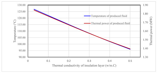
Figure 6.
Effect of insulation layer’s thermal conductivity on the temperature and thermal power of the produced fluid.
Figure 7 shows the effect of the insulation layer’s thickness on the temperature and thermal power of the produced fluid. It demonstrates that the temperature and thermal power of the produced fluid increase with the thickness of the insulation layer in the fluid production wellbore. This is expected, because less heat in the fluid is lost to the surrounding formation rock during its flow up the insulated wellbore.
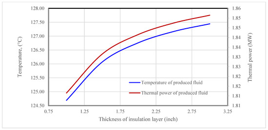
Figure 7.
Effect of insulation layer thickness on the temperature and thermal power of the produced fluid.
Figure 8 presents two curves to show the effect of fracture width on the temperature and thermal power of the produced fluid. It shows that the temperature of the produced fluid increases with the fracture width. This is expected, because for a given fluid flowrate, the fracture width determines the area of the formation that is available to the fluid. Thus, increasing the fracture width increases the area of the fracture network that the fluid interacts with, resulting in greater heat transfer from fractures to the fluid.
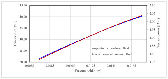
Figure 8.
Effect of fracture width on the temperature and thermal power of the produced fluid.
Figure 9 shows the effect of the number of fractures on the temperature and thermal power of the produced fluid. It indicates an effect which is like that of the fracture width. The temperature of the produced fluid increases with the number of fractures due to the short retention time of fluid in the fractures when multiple fractures share the same total fluid flow rate.
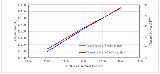
Figure 9.
Effect of number of fractures on the temperature and thermal power of the produced fluid.
This study focuses on the shale gas field in the Haynesville area, northwestern Louisiana in the United States selected according to the heat flow map presented by Blackwell et al. [6]. The heat flow in the gas field is very similar to that in North Dacota [7,8,9]. The studied well structure (fractured well pair) is a modified version of U-shaped well proposed by Liao et al. [10]. The heat energy productivity of the U-shaped well was thoroughly studied by other investigators including Ma et al. [11], Riahi et al. [12], Schulz [13], and Sun et al. [14]. The temperature and thermal power data presented in Figure 3, Figure 4, Figure 5, Figure 6, Figure 7, Figure 8 and Figure 9 show that the newly proposed fractured well pairs are more beneficial than the U-shaped wells. This is attributed to the higher efficiency of heat transfer in fractures than in wellbores.
3. Conclusions
An innovative mathematical model was developed in this work to simulate heat transfer in fracture-connected well pairs. The model was used to investigate factors affecting the heat energy productivity of geothermal wells that have been converted from hydrocarbon wells. Model analysis for a well pair in northwest Louisiana allows for drawing the following conclusions:
- As a result of the continuous heat transfer from the rock matrix to the injected work fluid, over time, both the temperature and thermal power of the produced fluid drop significantly. If the flowing work fluid is in constant contact with the formation rock without allowing for heat regeneration, the temperature of the produced fluid will be greater than 125 °C in the first three years, which is much higher than the 75 °C required for electricity generation with ORC technology.
- Increasing the fluid flow rate will decrease the temperature of the produced fluid due to the reduced residence time within the fractures. However, the thermal power of the produced fluid will increase because of the increased fluid mass flow rate.
- Insulation of the fluid production wellbore is necessary to reduce heat loss back to the formation rock. Reducing thermal conductivity and increasing the thickness of the insulation layer will effectively cut down the heat loss. Both the temperature and thermal power of the produced fluid will be enhanced by wellbore insulation.
- For a given height, the fracture width determines the area that is available to the fluid. Increasing the fracture width will also increase the fluid retention time in the fracture and thus the heat transfer from the formation rock to the fluid in the fracture.
- At a given fluid flowrate, increasing the number of identical fractures will increase the area of the fractures and fluid retention time in the fractures. Higher heat transfer efficiency from the formation rock to the work fluid is expected, and a higher temperature and thermal power of the produced fluid are anticipated.
Author Contributions
Conceptualization, B.G.; Methodology, B.G.; Software, B.G. and E.E.; Validation, B.G.; Investigation, B.G.; Resources, B.G.; Data curation, E.E.; Writing—original draft, B.G.; Writing—review & editing, E.E.; Visualization, E.E.; Supervision, B.G.; Project administration, B.G.; Funding acquisition, B.G. All authors have read and agreed to the published version of the manuscript.
Funding
This work was funded by the State of Louisiana BoRSF through the project “Conversion of End-of-Life Oil Wells to Geothermal Energy Wells: A Heat Transfer Enhancement Study,” grant No. LEQSF (2024-27)-RD-B-04.
Institutional Review Board Statement
Not applicable.
Informed Consent Statement
Not applicable.
Data Availability Statement
The original contributions presented in this study are included in the article. Further inquiries can be directed to the corresponding author.
Conflicts of Interest
The authors declare no conflict of interest.
Appendix A. Derivation of Mathematical Model for Transient Heat Transfer from Rock Formations to Hydraulic Fractures
Figure 2 illustrates a condition of one-dimensional heat transfer from the solid to the fluid inside a hydraulic fracture (shaded region). The heat flow rate at the surface of the fracture is given by a classic solution of the following form [15]:
where Q0 is the heat flow rate in J/s, K is the thermal conductivity of the solid in W/m-C, A is the total area for heat flow in m2, a is the thermal diffusivity of the solid in m2/s, t is time in s, Ti is the initial temperature of the solid in °C, and Tf is the constant fluid temperature at the surface of the solid in °C.
For the condition shown in Figure 2, the total area for heat flow is expressed as
where h and L are the height and length of the fracture in m, respectively. Therefore, Equation (A1) becomes
If the fluid enters the fracture at time t1 and leaves the fracture at time t2, the heat energy transferred from the solid to the fluid is expressed as
which is integrated to obtain the following:
If the fluid enters the fracture with a temperature T0 and leaves the fracture with a temperature Tx, the heat energy gained by the fluid is expressed as
where is the heat energy gained by the fluid in J, Cp is the specific heat of the fluid in J/kg-°C, and m is the mass of the fluid in the fracture in kg. The mass of fluid in the fracture is further expressed as
where r is the fluid density in kg/m3, w is the fracture width (aperture) in m, and is the fracture porosity in the volume fraction. Substituting Equation (A7) into Equation (A6) yields
Assuming that , Equation (A5) is modified to get
Because the energy balance dictates , Equations (A8) and (A9) give
which solves the temperature at the exit of the fracture as
References
- Abudureyimu, S. Geothermal Energy from Repurposed Oil and Gas Wells in Western North Dakota. Master Thesis, University of North Dakota, Grand Forks, ND, USA, 2020. Available online: https://commons.und.edu/theses/3087 (accessed on 1 March 2025).
- Wei, N.; Guo, B. Deliverable Wellhead Temperature—A Feasibility Study of Converting Abandoned Oil/Gas Wells to Geothermal Energy Wells. Sustainability 2023, 15, 729. [Google Scholar] [CrossRef]
- Zhang, P.; Guo, B. Factors Affecting the Fluid Temperature of Geothermal Energy Wells Converted from Abandoned Oil/Gas Wells. Adv. Geo-Energy Res. 2023, 9, 5–12. [Google Scholar] [CrossRef]
- Zhang, P.; Guo, B. A Feasibility Assessment of Heat Energy Productivity of Geothermal Wells Converted from Oil/Gas Wells. Sustainability 2024, 16, 768. [Google Scholar] [CrossRef]
- Guo, B.; Song, S.; Ghalambor, A.; Lin, T. Offshore Pipelines, 2nd ed.; Elsevier: Oxford, UK, 2014; pp. 367–373. [Google Scholar]
- Blackwell, D.D.; Richards, M.C.; Frone, Z.S.; Batir, J.F.; Williams, M.A.; Ruzo, A.A.; Dingwall, R.K. SMU Geothermal Laboratory Heat Flow Map of the Conterminous United States. 2011. Supported by Google.org. Available online: http://www.smu.edu/geothermal (accessed on 1 March 2025).
- Gosnold, W.; Abudureyimu, S.; Tisiryapkina, I.; Wang, D.; Ballestero, M. The Potential for Binary Geothermal Power in the Williston Basin. GRC Trans. 2019, 43, 114–126. [Google Scholar]
- Gosnold, W.; Ballesteros, M.; Wang, D.; Crowell, J. Using Geothermal Energy to Reduce Oil Production Costs. GRC Trans. 2020, 44. Available online: https://commons.und.edu/gge-fac/6/ (accessed on 1 March 2025).
- Gosnold, W.; Mann, M.; Salehfar, H. The UND-CLR Binary Geothermal Power Plant. GRC Trans. 2017, 41, 1824–1834. [Google Scholar]
- Liao, Y.; Sun, X.; Sun, B.; Wang, Z.; Wang, J.; Wang, X. Geothermal Exploitation and Electricity Generation from Multibranch U-Shaped Well-Enhanced Geothermal System. Renew. Energy 2021, 163, 2178–2189. [Google Scholar] [CrossRef]
- Ma, Y.; Li, S.; Zhang, L.; Liu, S.; Wang, M. Heat extraction performance evaluation of U-shaped well geothermal production system under different well-layout parameters and engineering schemes. Renew. Energy 2023, 203, 473–484. [Google Scholar] [CrossRef]
- Riahi, A.; Moncarz, P.; Kolbe, W. Innovative Closed-Loop Geothermal Well Designs Using Water and Super Critical Carbon Dioxide as Working Fluids; Stanford University: Stanford, CA, USA, 2017. [Google Scholar]
- Schulz, S.U. Investigations on the Improvement of the Energy Output of a Closed Loop Geothermal System (CLGS). Ph.D. Thesis, Technical University of Berlin, Berlin, Germany, 2008. [Google Scholar]
- Sun, F.; Yao, Y.; Li, G. Geothermal Energy Development by Circulating CO2 in a U-shaped Closed Loop Geothermal System. Energy Convers. Manag. 2018, 174, 971–982. [Google Scholar] [CrossRef]
- Holman, J.P. Heat Transfer, 5th ed.; McGraw-Hill Book Company: New York, NY, USA, 1981; pp. 115–118. [Google Scholar]
Disclaimer/Publisher’s Note: The statements, opinions and data contained in all publications are solely those of the individual author(s) and contributor(s) and not of MDPI and/or the editor(s). MDPI and/or the editor(s) disclaim responsibility for any injury to people or property resulting from any ideas, methods, instructions or products referred to in the content. |
© 2025 by the authors. Licensee MDPI, Basel, Switzerland. This article is an open access article distributed under the terms and conditions of the Creative Commons Attribution (CC BY) license (https://creativecommons.org/licenses/by/4.0/).