Pre-Insertion Resistor Temperature Prediction Based on a Novel Loss Function Combining Deep Learning and the Finite Element Method

Abstract

During transmission line faults, the pre-insertion resistors in circuit breakers accumulate heat and lead to thermal explosion during repeated closing. The risk of thermal explosion can be reduced if the pre-insertion resistor temperature can be accurately predicted. This study proposes a method for predicting the pre-insertion resistor temperature to optimize the cooling time. The overfitting problem is more serious for models using traditional loss functions. To solve this problem, deep learning models based on a new loss function, the rational smoothing loss, are used to predict the temperature of pre-insertion resistors. The rational smoothing loss, inspired by the kernel function, dynamically adjusts the error versus gradient and incorporates constraints for regularization. The coati optimization algorithm with Ornstein–Uhlenbeck mutation optimizes the rational smoothing loss parameters. The results demonstrate that models using rational smoothing loss significantly outperform those with traditional loss functions, showing reductions of 77.97% in mean absolute error and 93.72% in mean square error, reducing the mean absolute error to 0.29 K. Additionally, the prediction curves exhibit remarkable smoothness, indicating the rational smoothing loss’s robustness against overfitting. The accurate prediction of pre-insertion resistor temperature is crucial for safely operating circuit breakers and technically supporting cooling time optimization.

1. Introduction

Rapid economic growth has driven the demand for more efficient and reliable electrical networks, making the development of ultra-high-voltage (UHV) and extra-high-voltage (EHV) transmission systems increasingly critical. Concurrently, pre-insertion resistors (PIRs) are now more widely incorporated in the design of electrical switches, including gas-insulated switches (GISs), hybrid gas-insulated switches (HGISs), and oil circuit breakers [1,2]. In circuit breaker operations, PIRs play a key role in mitigating inrush currents and transient over-voltage during switching. This has led to increased research focus on their dynamic thermal and electrical behavior in high-voltage systems [3].

In a series of innovative studies, researchers have explored and advanced PIR’s power testing, synchronous switching technology, applications in other areas, and failure analysis to gain insight into its potential to improve system reliability and performance in a variety of situations.

H. Heiermeier et al. [4] proposed an alternative approach for the power testing of PIRs that aims to preserve their critical parameters. This method involves six key steps: assessing the mechanical insertion time and the dielectric strength decay rate, calculating the maximum energy of the PIR and its electrical insertion time (EIT), identifying the most adverse network conditions for testing, determining the adjusted EIT and resistor stack length necessary for the equivalent PIR test, and evaluating the new EIT and corresponding PIR energy and the “pre-arc” behavior of the PIR switch. This provides a complete and effective test procedure for PIR. To mitigate transient voltages during the switching of shunt power capacitor compensators, R. Sun et al. [5] introduced synchronized switching techniques incorporating PIR for use in ultra-high-voltage transmission systems. Their study identified that factors such as the closing target angle, resistor insertion time, and resistor size are significant contributors to switching transients in both single-bank and back-to-back switching configurations. Kunal A. Bhatt et al. [6] demonstrated that the use of a controlled switching device with PIR-CB can effectively reduce the asymmetric DC component in the charging current during the energization of a shunt reactor. This reduction is achieved by optimizing the insertion timing, resistor value, and EIT of the PIR. The simulation outcomes were also validated via comparison with field data, confirming the practical feasibility of the proposed approach in real-world applications. The fast transient overvoltage generated by the operation of the disconnecting switch influences the number of premature failures of the current transformer. By applying a PIR of 1000 Ω to the disconnecting switch, simulations show that it is possible to reduce the overvoltage value to the standard limit and also significantly reduce the rate of rise in the voltage waveform [7]. S. Zondi et al. [8] simulated the transient voltage during capacitor bank switching with an electromagnetic transient program, and the simulation results showed that the PIR method can significantly reduce this transient phenomenon. L. He [9] developed a generalized model of a modular multilevel converter (MMC) for high-voltage DC, and the simulation results proved that a PIR can effectively suppress the inrush current of the converter transformer. A method [10] is presented for determining the optimum value of a PIR to minimize the increasingly frequent current drifts and switching over-voltage that occur in high-voltage cables in frequent-use scenarios. H. Shi et al. [11] conducted simulations to analyze the transient currents under three fault conditions in relation to PIRs: short circuit, breakdown, and open circuit. Their findings revealed that parameters such as the harmonic content of the inrush current, the timing of the peak inrush current, and the three-phase imbalance exhibit notable differences when compared to normal operating conditions. These variations can serve as useful indicators for fault diagnosis techniques.

These collective endeavors not only enhance understanding of PIR functionality within electrical systems but also pave the way for their optimized application, promising improved system stability and efficiency.

PIRs will heat up rapidly during the opening and closing process of the circuit breaker. However, due to the temperature limit of PIRs, repeated opening and closing operations of the circuit breaker may cause PIRs to be damaged by overheating. The opening and closing of circuit breakers are common operations in power system. At present, there is no temperature prediction for PIRs, which leads to their frequent damage. Temperature prediction is an important indicator for determining whether a circuit breaker can perform opening and closing operations. Few studies have considered the thermal characteristics of PIRs under fault conditions and their implications for system reliability [12]. In particular, thermal damage caused by electric–thermal coupling during fault-induced closures is a major risk factor, yet it has not been extensively studied. However, there are very few studies on the temperature rise in PIRs. Most existing works focus on electromagnetic or mechanical behaviors, while temperature prediction remains underexplored despite its critical impact on failure modes [12]. During closing, the PIR accumulates heat due to the passage of the current, causing its internal temperature to rise. When a transmission line fault occurs, the PIR may be broken due to multiple closures. If the temperature of the PIR can be accurately measured, then the closing interval can be increased to extend the cooling time when the PIR temperature is too high, which will effectively prevent the PIR from breaking and then ensure the stable operation of the transmission line. Due to the high-voltage environment in which PIRs function, direct temperature measurement using sensors is not feasible. Moreover, the heating and cooling cycles of PIRs involve complex, nonlinear, and tightly coupled processes influenced by various parameters, making precise mathematical modeling challenging. Therefore, this study employed deep learning models to predict the temperature of the PIR.

Nowadays, many models have been widely used in engineering prediction. Machine learning techniques have been widely used in fault detection for power system components such as transformers, supporting more intelligent and proactive condition monitoring [13]. In the early stages of predictive analytics, statistical models were extensively employed, exemplified by methodologies such as autoregressive integrated moving average (ARIMA [14]). These models, however, are primarily limited to handling linear data. To address this limitation, machine learning techniques like support vector regression (SVR [15]) and extreme gradient boosting (XGBoost, Python 3.8 [16]) emerged as solutions for extracting nonlinear patterns from time series data. Machine learning methods have been proven effective in similar predictive tasks for other substation equipment, enhancing fault prevention and system reliability [17].

The effectiveness of AI-driven control and prediction strategies has already been demonstrated in the management of distributed energy systems [18]. With the advancement of artificial intelligence, plenty of models have been developed for predictive tasks, among which recurrent neural network (RNN)-based models have gained popularity, such as long short-term memory (LSTM [19]) and gated recurrent unit (GRU [20]) models. The LSTM model, through its intricate design involving input, forget, and output gates, effectively captures temporal information, mitigating the gradient vanishing/exploding issues inherent to traditional RNN [21]. Conversely, the GRU model simplifies the LSTM architecture while maintaining comparable predictive performance. Furthermore, other models, including those based on the Transformer [22] (Informer [23]), multi-layer perceptron (MLP [24]), MLP-based models (Dlinear [25], Frets [26]), convolutional neural network (CNN [27,28,29]), and CNN-based models (MICN [30], TimesNet [31]), have also been applied to predictive tasks such as temperature forecasting.

However, much research has focused on model improvement, with less attention paid to the training process. Commonly used traditional loss functions are sensitive to outliers and prone to overfitting due to their linearly increasing gradients with prediction errors. This often leads to diminished model accuracy on test datasets. To address this issue, this study proposes the rational smooth loss function (RSL), inspired by the principle of kernel function. RSL dynamically adjusts gradients and incorporates regularization terms to mitigate overfitting, offering a refined approach to enhancing predictive model performance.

Predicting PIR temperature using deep learning models requires a large amount of data. However, there is less data available on the temperature rise of the PIR. Moreover, conducting experiments on the PIR is very costly. To obtain a large amount of data, a large number of simulations are performed using finite element simulation to obtain a dataset. The finite element method (FEM) is a computational technique used to approximate the solution of complex systems in various domains. It has already shown effectiveness in simulating a PIR’s internal thermal and electrical fields, especially when considering microstructural influences like porosity [32]. By discretizing the domain into elements and interpolating using shape functions, FEM achieves a high degree of accuracy in modeling physical phenomena under a variety of boundary conditions, making it an indispensable method for engineering and scientific simulations. Compared to other methods (finite difference method and finite volume method), FEM has more advantages. It is very suitable for dealing with complex geometries and heterogeneous materials. FEM uses meshing, which allows the flexible adjustment of the mesh density to improve the accuracy of the model and is especially suitable for irregular shapes and boundaries. FEM has excellent multi-physics field coupling capability, enabling it to effectively simulate multiple interacting physical processes such as electromagnetic fields, thermal fields, hydrodynamics, etc., which is crucial for PIR simulations.

The rest of this article is organized as follows:

Section 2 describes the LSTM, GRU, and BP models.

Section 3 describes the novel loss function RSL.

Section 4 describes the population intelligent optimization algorithm, COA, and its improvement strategy used to find the RSL parameters.

Section 5 describes the finite element simulation model and presents the prediction results of the three algorithms after using RSL.

2. Deep Learning Models

2.1. Long Short-Term Memory

Long short-term memory (LSTM), a sophisticated model in the realm of deep learning, is intricately designed for the nuanced processing of sequential data. This network emerges as a solution to the persistent challenge of gradient vanishing that plagues recurrent neural networks (RNNs) during the handling of extended sequences. By incorporating a gating mechanism, LSTM is adept at capturing and regulating long-term dependencies within sequence data. Central to its architecture is the cell state, an internal memory unit with the capability to modify information through addition, deletion, and updates, dependent on both the input data and its existing state. Furthermore, the LSTM network is equipped with three distinct gating units: the forget gate, input gate, and output gate. These units play a pivotal role in determining the updates to the cell state and the direction of information flow via a learnable gating mechanism. This innovation enables the LSTM network to efficiently manage long-term dependencies in sequences, leading to its exceptional performance across a diverse range of tasks.

2.2. Gated Recurrent Unit

A gated recurrent unit (GRU) presents an evolution in deep learning models for sequence modeling, paralleling the LSTM network with a shared objective to address the gradient vanishing problem inherent in traditional RNNs. The GRU streamlines the LSTM architecture by integrating the functionality of forgetting and input gates into a unified mechanism known as “update gates”, while also consolidating the cell and hidden states into single entities termed “states”. This refinement reduces the architectural complexity found in LSTM, resulting in a model that is not only more compact but also characterized by a reduced parameter count. Consequently, a GRU network offers advantages in terms of training efficiency and has demonstrated superior performance across a variety of sequence modeling tasks. The simplified gating mechanism and structural elegance of GRUs render them more amenable to training and fine-tuning in certain contexts.

2.3. Backpropagation

Backpropagation (BP) neural networks stand as a cornerstone within the domain of deep learning, particularly for tackling supervised learning challenges. These networks are architecturally composed of multiple layers, including input, hidden, and output strata. Employing the backpropagation algorithm, BP neural networks are adept at assimilating knowledge from training data, enabling the adjustment of network parameters to narrow the discrepancy between predicted outputs and actual labels—a process central to optimizing the loss function. In essence, BP neural networks ascertain the gradient of the loss function relative to network parameters through chain derivation, proceeding to update these parameters via a gradient descent algorithm. BP neural networks exhibit commendable performance across a myriad of machine learning tasks.

3. The Rational Smooth Loss Function

The traditional methods to avoid overfitting are generally regularization, dropout, early stopping, and cross-validation. In this paper, a novel loss function is designed to avoid overfitting. Since the temperature at which the PIRs need to be predicted is nonlinear, using the common L1 and L2 paradigms as model optimization objectives may not accurately portray the predicted nonlinearity. A common approach is to map the data to higher dimensions using a kernel function [33,34]. This does not add much computational complexity to map the data to a higher dimensional space. Assuming that $f$ is a nonlinear mapping, the kernel function can be denoted as follows:

$$K(y,y^{\prime })=<f(y),f(y^{\prime })>.$$

(1)

The rational quadratic loss function (RQL) may be used as a mapping function:

$$K(y,y^{\prime })={\displaystyle \frac{a}{{(y-y^{\prime })}^2+a}},$$

(2)

where $a$ is a hyperparameter. Thus, the RQL is

$$L_{RQL}=1-K(y,y^{\prime })={\displaystyle \frac{{(y-y^{\prime })}^2}{{(y-y^{\prime })}^2+a}},$$

(3)

where $y^{\prime }$ is the prediction value and $y$ is the true value. A Maclaurin expansion [35] is conducted for $L_{RQL}$:

$$L_{RQL}={\displaystyle \sum _{i=1}^{\infty }{(-1)}^{i+1}\frac{{(y-y^{\prime })}^{2i}}{a^i}}.$$

(4)

Note that the RQL has a lowest subterm of 2, which may lose some low-dimensional (linear) information. Therefore, this study transforms RQL into a rational primary loss function (RPL). The RPL can be described as follows:

$$L_{RPL}={\displaystyle \frac{\left|y-y^{\prime }\right|}{\left|y-y^{\prime }\right|+a}}.$$

(5)

Since RPL is not derivable at 0, the Maclaurin expansion cannot be performed directly. Thus, consider finding a point in the right neighborhood (math.) of 0, (0, c), c > 0 for Taylor expansion, when c is small enough. The Taylor expansion [36] is approximated using the following equation:

$$L_{RPL}\approx {\displaystyle \frac{\left|y-y^{\prime }\right|}{a}}+{\displaystyle \sum _{i=2}^{\infty }{(-1)}^{i+1}\frac{{(y-y^{\prime })}^i}{a^i}}.$$

(6)

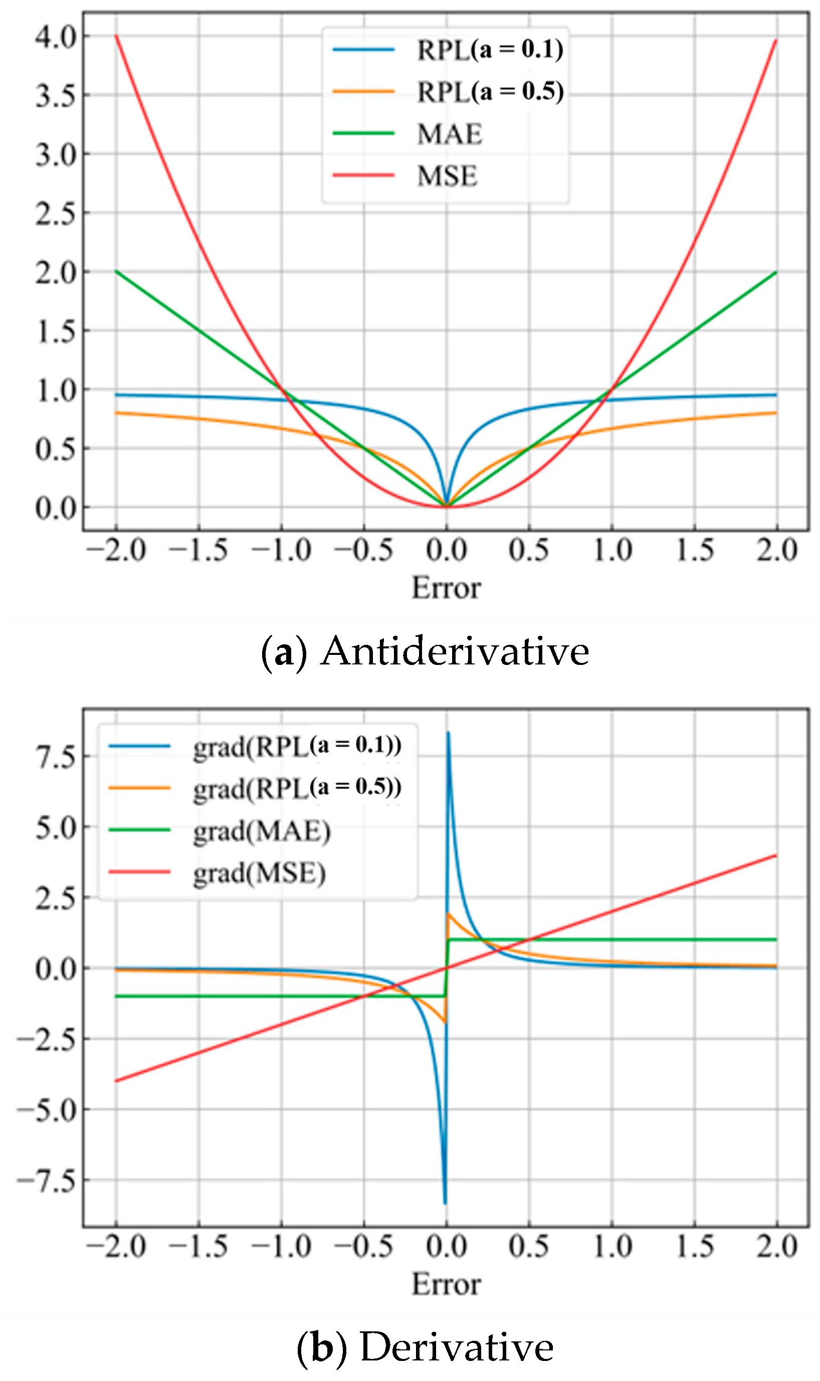
Both low and high subterms can be found, and the original data can be adequately mapped to each dimension. From Figure 1, it can be found that the gradient of RPL increases and then decreases with the error: the gradient is sensitive to the error within a certain range, and when the error is too high (anomaly), the gradient is less sensitive to the error, which suppresses the effect of the outliers on the optimization of the model. Unlike the MSE and MAE, it greatly reduces the sensitivity of the model to outliers, enhances the generalization performance of the model, and is less prone to overfitting.

In addition, the outlier effect is inevitably encountered during model training. To address this issue, regular terms that constrain the predicted values are added. In the formulation of the loss function, the integration of L1 and L2 constraints on the model’s predicted values introduces a nuanced approach to regulating these predictions. These constraints foster the sparsity of the predicted values within the parameter space of the model, a property that is advantageous for both selecting relevant features and diminishing noise interference. Concurrently, by moderating the magnitude of these predictions, the model safeguards against overfitting, curtails the impact of outliers, and ensures the stability of gradient descent. This strategy enhances the model’s interpretability and generalizability, thereby bolstering its resilience to noise and outliers and yielding more robust and efficacious outcomes in both model training and prediction phases. It renders the model more intelligible and adaptable, ensuring its efficacy in real-world scenarios. However, the regular term coefficients should not be too large. However, it is critical to calibrate the coefficients of these constraints carefully to prevent them from overshadowing the loss function, which could otherwise result in trivial predictions. Here is the formula for the rational smooth loss function (RSL):

$$L_{RSL}={\displaystyle \frac{1}{n}}{\displaystyle \sum _{i=1}^n\frac{\left|y_i-y_i^{\prime }\right|}{\left|y_i-y_i^{\prime }\right|+a}}+b·{\displaystyle \frac{1}{n}}{\displaystyle \sum _{i=1}^n\left|y_i^{\prime }\right|}+c·{\displaystyle \frac{1}{n}}{\displaystyle \sum _{i=1}^n{y_i^{\prime }}^2}$$

(7)

where $b$ and c are hyperparameters of $L_{RSL}$, and n is the length of the prediction sequence.

4. Improved Coati Optimization Algorithm

4.1. Coati Optimization Algorithm

There are three parameters in RSL: a, b, and c. To find the optimal parameters in a better way, this study uses the population intelligent optimization algorithm. The coati optimization algorithm (COA) was proposed in 2023 and has high search capacity and fast convergence [37].

4.1.1. Phase 1: Hunting and Attacking Strategy on Iguana (Exploration Phase)

This strategy, emulated within the algorithm, involves half of the coatis climbing a tree to displace and intimidate the target—represented in the algorithm as the iguana—while the remainder wait below for the prey to fall. This coordinated approach facilitates the coatis’ strategic relocation across the search space, showcasing the COA’s capability for extensive global exploration within the problem-solving landscape.

In the design of the COA method, the location of the iguana is assumed to be the location of the best member of the coati population. Therefore, the position of the coatis when climbing trees can be described by Equation (8) as follows:

$$\begin{array}{l}{X}_i^{P1}:x_{i,j}^{P1}=x_{i,j}+r·(Iguan{a}_j-I·x_{i,j}),\\ \mathrm{for} i=1,2,\dots ,{\displaystyle \frac{N}{2}},j=1,2,\dots ,m.\end{array}$$

(8)

After falling on the ground, the iguana is placed at a random position in the search space. Based on this random position, the coatis on the ground move through the search space, modeled as in Equations (9) and (10):

$$Iguan{a}^G:Iguan{a}_j^G=l{b}_j+r·\left(u{b}_j-l{b}_j\right),j=1,2,\dots ,m,$$

(9)

$$\begin{array}{l}{X}_i^{P1}:x_{i,j}^{P1}=\left\{\begin{array}{rr}\hfill x_{i,j}+r·\left(Iguan{a}_j^G-I·x_{i,j}\right),& \hfill F_{Iguan{a}^G}<F_i,\\ \hfill x_{i,j}+r·\left(x_{i,j}-Iguan{a}_j^G\right),& \hfill else,\end{array}\right.,\\ \mathrm{for} i=⌊{\displaystyle \frac{N}{2}}⌋+1,⌊{\displaystyle \frac{N}{2}}⌋+2,\dots ,N,j=1,2,\dots ,m.\end{array}$$

(10)

A new position is computed for each coati, and if the new position improves the value of the objective function, the updated position is used as the position of the coati. Otherwise, the coati remains in its previous position. This process is represented by Equation (11):

$$X_i=\left\{\begin{array}{rr}{X}_i^{P1},\hfill & \hfill F_i^{P1}<F_i,\\ X_i,\hfill & \hfill else.\end{array}\right.$$

(11)

Here, $X_i^{P1}$ represents the updated position for the i-th coati; $x_{i,j}^{P1}$ is its j-th dimension; $F_i^{P1}$ is the objective function value at this position; r is a random real number selected from the interval [0, 1]; $Iguana$ indicates the position of the iguana in the search space, which refers to the position of the best solution found; $Iguan{a}_j$ is its j-th dimension; $I$ is an integer randomly chosen from the set {1,2}; $Iguan{a}^G$ is the position of the iguana on the ground, which is randomly generated; $Iguan{a}_j^G$ is its j-th dimension; $F_{Iguan{a}^G}$ is its value of the objective function; and $⌊·⌋$ is the floor function (also referred to as the greatest integer function).

4.1.2. Phase 2: The Process of Escaping from Predators (Exploitation Phase)

The second phase focuses on updating the coatis’ positions within the search space. This update is modeled mathematically to reflect the natural behavior of coatis when they encounter and flee from a predator. When a predator approaches, the coati moves away from its current location. In this approach, the coati’s response results in a shift to a nearby, safer position, illustrating the COA’s capacity for local search.

To simulate this behavior, random positions are generated near each coati position with Equations (12) and (13):

$$l{b}_j^{local}={\displaystyle \frac{l{b}_j}{t}},u{b}_j^{local}={\displaystyle \frac{u{b}_j}{t}},\mathrm{where} t=1,2,\dots ,T.$$

(12)

$$\begin{array}{l}{X}_i^{P2}:x_{i,j}^{P2}=x_{i,j}+\left(1-2r\right)·\left(l{b}_j^{\mathrm{local}}+r·\left(u{b}_j^{\mathrm{local}}-l{b}_j^{\mathrm{local}}\right)\right),\\ i=1,2,\dots ,N,j=1,2,\dots ,m\end{array}$$

(13)

If the newly calculated position improves the value of the objective function, then the updated position is used, and this condition is simulated using Equation (14):

$$X_i=\left\{\begin{array}{rr}{X}_i^{P2},\hfill & \hfill F_i^{P2}<F_i,\\ X_i,\hfill & \hfill else,\end{array}\right.$$

(14)

Here, $X_i^{P2}$ represents the updated position of the i-th coati, determined in the second phase of the COA; $x_{i,j}^{P2}$, its j-th dimension; $F_i^{P2}$, the objective function value at this position; r, a random number selected from the interval [0, 1]; t, the iteration index; $l{b}_j^{local}$ and $u{b}_j^{local}$, the local lower and upper bounds, respectively, of the j-th decision variable; and $l{b}_j$ and $u{b}_j$, the global lower and upper bounds for the j-th decision variable.

4.2. Ornstein–Uhlenbeck Mutation

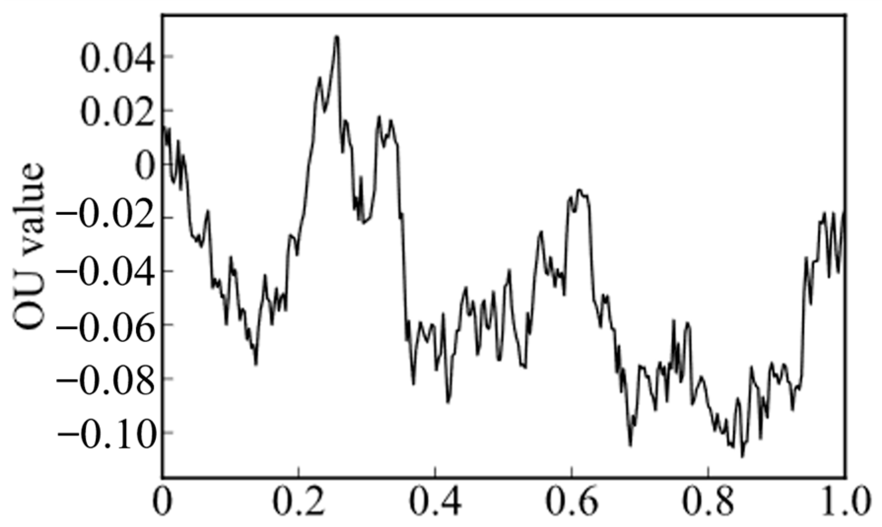
Traditional mutation techniques commonly employ distributions such as the normal distribution [38] and Cauchy distribution [39,40,41]. However, these distributions are inherently limited, as their positive probabilities restrict mutation directions to only positive values. This does not accommodate the need for mutations in the negative direction. In contrast, the Ornstein–Uhlenbeck (OU) process introduces randomness while allowing for both positive and negative fluctuations, and it inherently incorporates temporal correlation. An example of such a stochastic process is depicted in Figure 2. It is evident that the OU process can produce both positive and negative outcomes, making it a more suitable candidate for mutation perturbations.

$$X^{t+1}=X_{best}·(1+OU[B])$$

(15)

$$B=t\times M\times \left[C_1/(t_{\max }\times N)\right]$$

(16)

Here, $OU$ represents the value derived from the Ornstein–Uhlenbeck process; $C_1$, the number of points sampled by the OU process along the horizontal axis; N, the number of coati populations; $M$, the position update for the M-th coati; $X_{best}$, the current optimal fitness; and $X^{t+1}$, the fitness value after mutation.

Although the mutation technique described above improves the algorithm’s ability to escape local optima, it does not ensure that the fitness of the newly mutated position will surpass that of the original position. To address this, after performing the perturbation mutation, a greedy strategy is employed to decide whether the position should be updated. This decision is made by comparing the fitness values of the original and mutated positions. The greedy criterion is defined as follows, where $f\left(x\right)$ represents the fitness value at a given position:

$${X^{\prime }}_{best}=\left\{\begin{array}{l}{X}^{t+1},f(X^{t+1})<f(X_{best})\\ X_{best},f(X^{t+1})\ge f(X_{best})\end{array}\right.$$

(17)

where ${X^{\prime }}_{best}$ denotes the fitness value deemed more favorable after the comparison.

4.3. Improved Coati Optimization Algorithm Performance Test

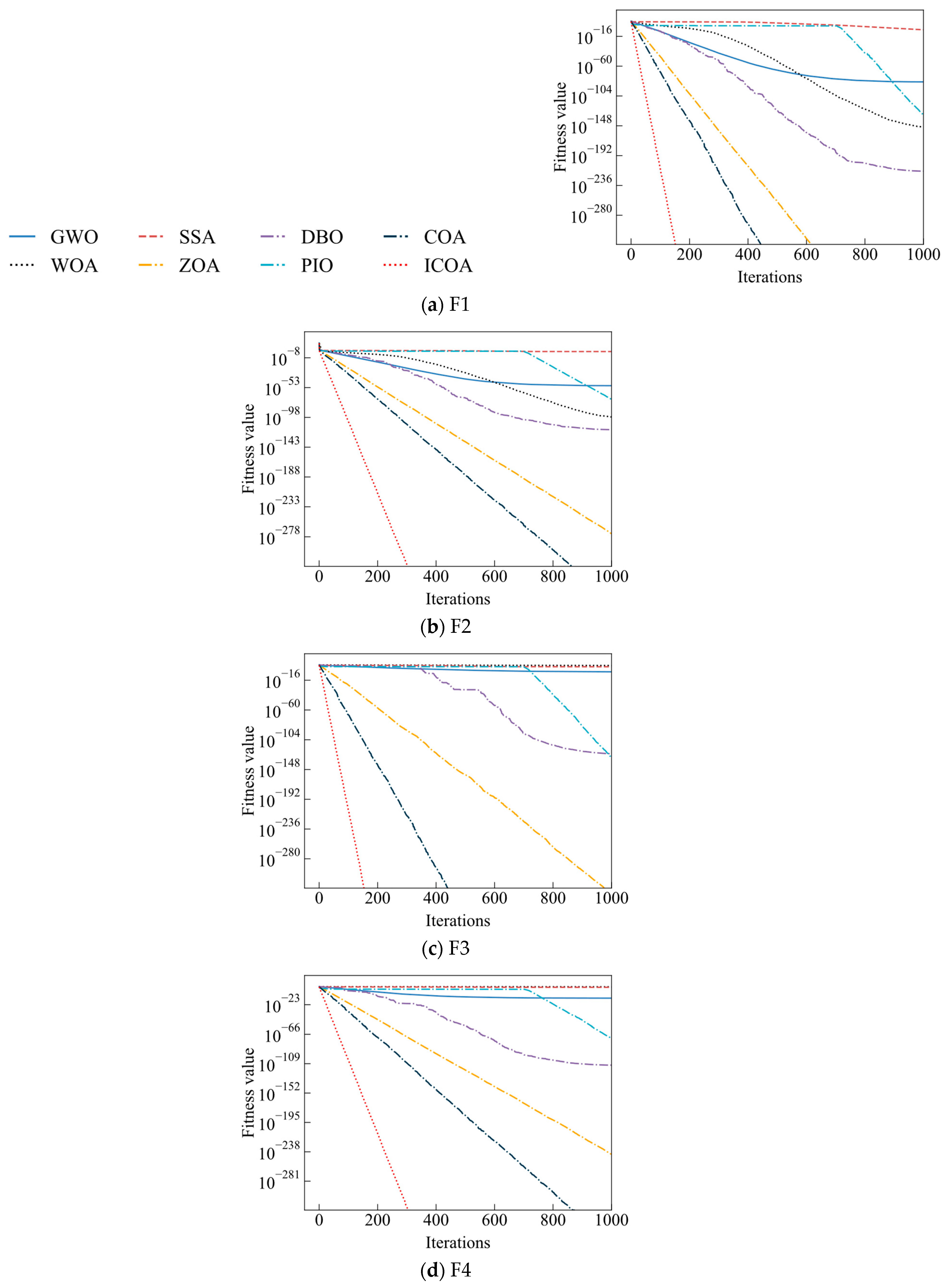
To ascertain the efficacy of the Improved coati optimization algorithm (ICOA), a comparative analysis was conducted utilizing four benchmark functions from the CEC2005 suite, against a backdrop of several contemporary algorithms: the gray wolf optimizer (GWO), sparrow search algorithm (SSA), dung beetle optimizer (DBO), COA, whale optimization algorithm (WOA), zebra optimization algorithm (ZOA), and pigeon-inspired optimization (PIO). The experimental setup was standardized with a population size of 30, dimensionality set at 30 for the test functions, a cap of 1000 iterations, and each test function subjected to 30 independent trials.

Table 1. Information on test functions.

Function		Dimension	Range	Optimal Value	Peak Value
F1	Sphere	30	[−100,100]	0	single peak
F2	Schwefel2.22	30	[−10,10]	0	single peak
F3	Schwefel1.2	30	[−100,100]	0	single peak
F4	Schwefel2.21	30	[−100,100]	0	single peak

presents an overview of the test functions, while Figure 3 delineates the convergence curve of the eight algorithms across these functions.

In the optimization of the rational smoothing loss (RSL) function, we set the search intervals and initial values for parameters a, b and c as follows: their initial values are in the ranges of [0.1, 10], [0, 1], and [0, 1] with the search intervals restricted to [0.1, 5], [0, 0.5], and [0.05, 0.5], respectively. These intervals were determined based on preliminary experiments, where smaller values for a and c provided better gradient adjustment and model stability, while b controlled the error smoothing.

The analyses reveal a pronounced enhancement in the convergence velocity of ICOA across functions F1-F4, compared to other algorithms. Within these test scenarios, ICOA demonstrated superior performance metrics, including mean, standard deviation, optimal value, and convergence velocity. These results not only underscore the potency of the adopted improvement strategy within ICOA but also suggest its pronounced capability in accelerating convergence and refining the search for optimal parameters. This study thereby affirms the advanced performance and application potential of ICOA in complex optimization landscapes. This is more helpful in optimizing the three parameters of the RSL.

5. Simulation Model—Finite Element Method and Dataset Acquisition

5.1. Working Principle of Circuit Breakers with PIR

When a circuit breaker is closed, if an unloaded line or a line restored after a fault is directly connected to the power system, sudden voltage change will trigger LC oscillation, generating an “switching overvoltage” that is much higher than the system’s rated voltage (usually reaching 2–4 times the rated voltage). This overvoltage poses a serious threat to the insulation performance of equipment such as line insulators, transformer windings, and capacitors. In severe cases, it may even cause insulation breakdown, leading to power system failures.

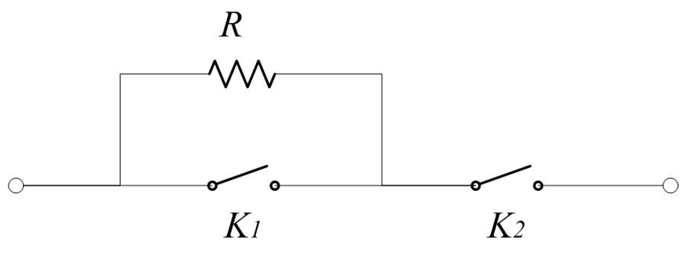
To prevent such failures, a PIR must be incorporated into the design of circuit breakers rated above 500 kV. A circuit diagram of the circuit breaker with the integrated closing resistor is shown in Figure 4.

In Figure 4, R represents the PIR, and K1 and K2 are the two switches of the circuit breaker. When the circuit breaker is closed, switch K2 is closed first. At this moment, the connection of the PIR can prevent the overvoltage caused by LC oscillation. Approximately 10 s after K2 is closed, switch K1 is then closed.

During the closing process, the PIR generates heat because current flows through it in a short period of time. If the circuit breaker undergoes multiple reclosing operations, the PIR may experience continuous temperature rise. When the temperature of the PIR exceeds its rated temperature range, it may explode, leading to circuit breaker damage. Therefore, predicting the temperature of the PIR is an important measure to prevent its explosion.

5.2. PIR Simulation Model

5.2.1. Basic Settings for Simulation

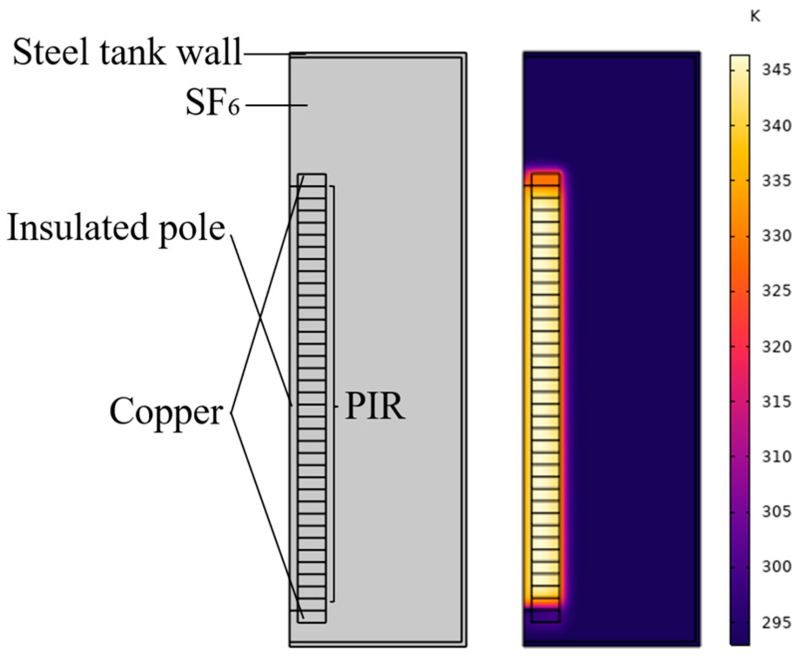
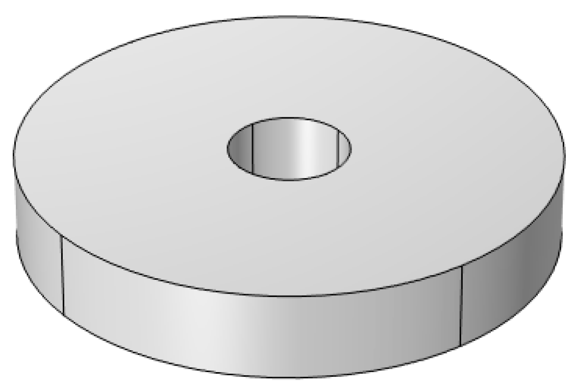
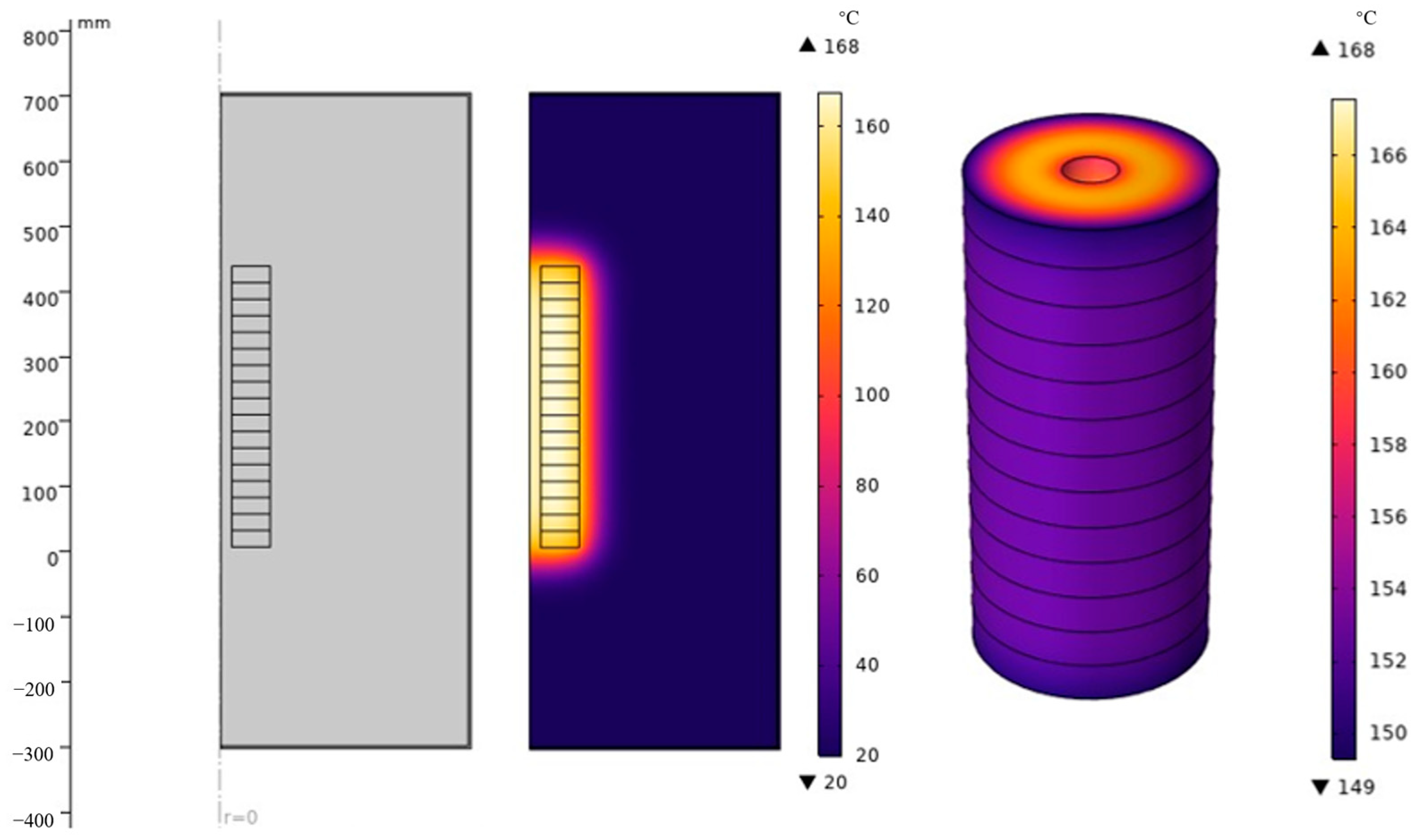
In this study, PIRs sourced from Morgan (UK) were subjected to a comprehensive simulation. Utilizing FEM software (COMSOL Multiphysics 6.1), a two-dimensional axisymmetric model was constructed (Figure 5), encompassing 35 PIRs, insulating rods, a steel enclosure, copper electrodes, and SF₆ [42]. The assembly of the multi-piece PIR, which is interconnected via bolting, negated the need for explicit modeling of the interstitial gaps in the simulation. Encapsulated within a steel casing, the space surrounding the PIR was filled with SF₆ gas, enhancing the insulation properties. The single PIR sheet was a hollow flat cylinder (Figure 6) with an outer diameter of 152 mm, an inner diameter of 34 mm, a thickness of 25.4 mm, and a resistance value of 5 Ω.

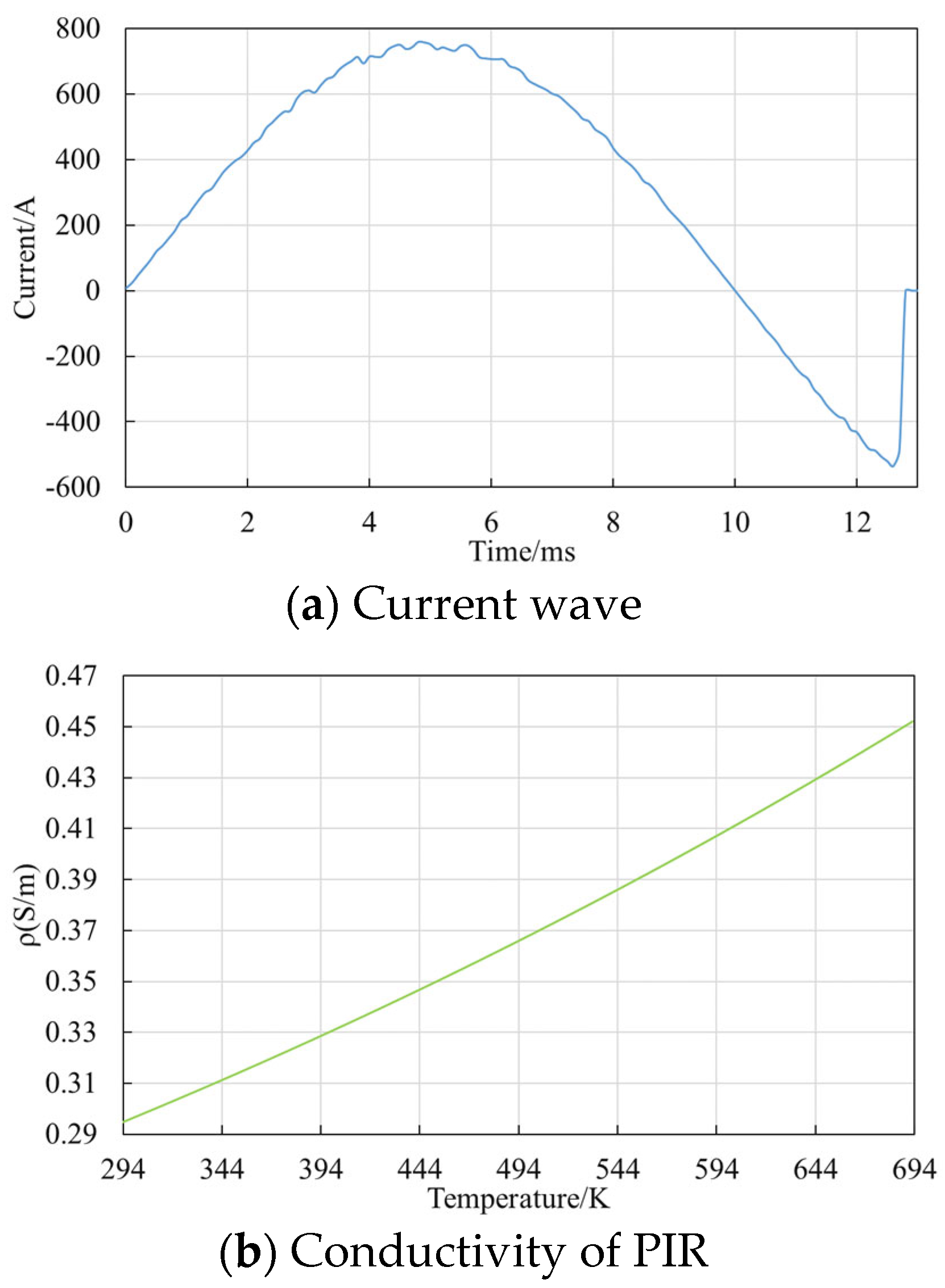
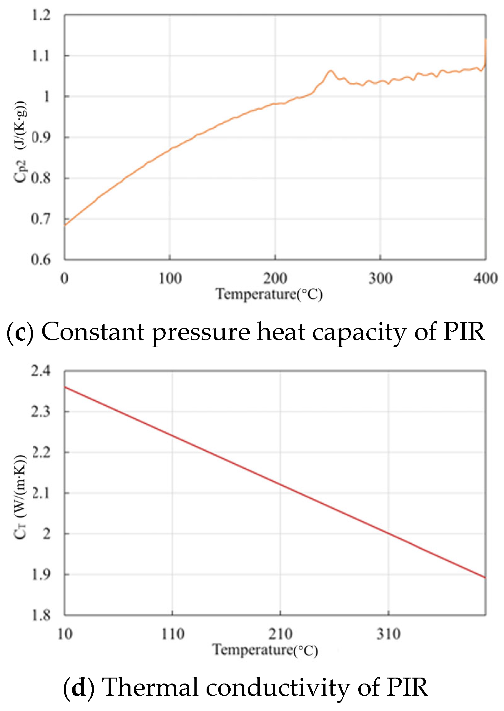
The underlying principle of the simulation is that when a substantial current flows through the PIR, significant heat is generated. The PIR, which becomes warmer than its surrounding environment, will exchange heat with nearby objects and the ambient surroundings through mechanisms such as conduction, convection, and thermal radiation. The entire simulation involves three main physical fields: electric, thermal, and flow fields. The interrelationship between these three physical fields is shown in Figure 7. The whole simulation process is divided into two steps: In the first step, the PIRs are energized with an approximate sinusoidal current with a starting phase of 0. In the second step, PIRs are cooled for 30 min. The thermal capacity of the 550 kV circuit breaker PIR was specified as follows: twice at two times the rated phase voltage, with a time interval of 30 min between the two times. Therefore, the cool simulation time was set to 30 min. In the simulation, there were four factors affecting the temperature of the PIR: current value, current duration, starting ambient temperature, and the initial temperature of the PIR itself. The physical parameters of the PIR, insulating rod [43,44], and SF₆ are shown in

Table 2. Physical parameters of the main substances.

Physical Parameter	PIR	Insulated Pole	SF6
Relative permittivity	5	——	——
Thermal conductivity/[W/(m·K)]	$C_T$	0.5	${\lambda }_g$
Constant pressure heat capacity/[J/(kg·K)]	$C_{p2}$	789.52	$C_{p1}$
Conductivity/[S/m]	$\rho$	——	——
Density/[kg/m3]	2250	2290	30
Kinetic viscosity/[Pa·s]	——	——	$\mu$

and Figure 8.

$${\lambda }_g=4.37e^{-3}-5.78e^{-5}T+4.79e^{-7}{T}^2-9.19e^{-10}{T}^3+8.18e^{-13}{T}^4-2.82e^{-16}{T}^5$$

(18)

$$C_{p1}=-218.4+4.73T+7.50e^{-3}{T}^2+5.67e^{-6}{T}^3-1.66e^{-9}{T}^4$$

(19)

$$\mu =2.88e^{-7}+5.51e^{-8}T-1.68e^{-11}{T}^2+1.39e^{-15}{T}^3$$

(20)

Here, $T, {\lambda }_g, C_p, \mu$ denote the temperature, thermal conductivity, constant pressure heat capacity, and kinetic viscosity of SF₆.

5.2.2. Setting of Range of Factors

The thermal capacity experiment for the 550 kV circuit breaker PIR component was conducted using a large sinusoidal current of 1600 A. The typical EIT of the PIR was between 8 and 12 ms. To enhance the diversity of the dataset, the current range was set between 200 A and 2500 A, while the input current duration varied from 7 ms to 13 ms. The temperature rise of the PIR was required to stay below 320 °C at an ambient temperature of 293 K. The minimum initial temperature was set to 20 °C, with the maximum initial temperature reaching 330 °C, which exceeds the permissible threshold for the PIR. Other factors, which have minimal impact, were neglected. The ranges of the variables are provided in

Table 3. The range of factors affecting temperature.

Variables		Range
Current	I/A	[200,2500]
Input current time	t1/ms	[7,13]
PIR temperature	To/°C	[20,330]
Environment temperature	T1/K	[293,603]

. In the finite element simulations, the mesh density cannot be infinitely refined, leading to occasional singular values, which may result in slight inaccuracies in predicting the maximum temperatures. The maximum temperature of the PIR is crucial for evaluating its operational state. Through numerous experiments, it was observed that after cooling, the temperature distribution becomes more uniform, with the maximum temperature closely aligning with the average value. Consequently, the temperatures simulated and predicted in this study are based on the average temperature of 35 PIR units.

5.2.3. Mesh and Output Time Size

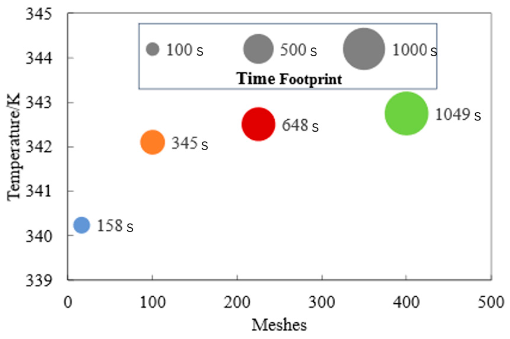
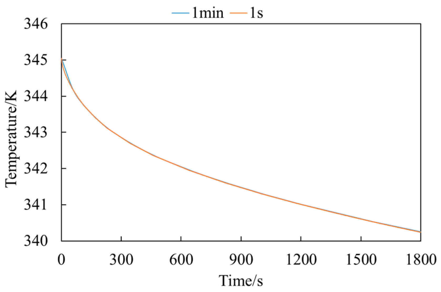
FEM software simulation is notably affected by the mesh size and output time step. A denser mesh enhances the computational burden, whereas a sparser mesh may reduce the accuracy of the results. This study meshed each resistor sheet into 4 × 4, 10 × 10, 15 × 15, and 20 × 20 meshes, and the software automatically generated meshes for the rest of the model. Examination of the outcomes (Figure 9) demonstrates that variations in mesh density yield only minor differences in temperature readings yet result in marked variations in computational duration. Given the scope of this investigation, which includes the simulation of 6000 datasets, a judicious compromise is required between precision and computational efficiency. Hence, a mesh size of 10 × 10 was selected to optimize the computational process while ensuring satisfactory accuracy. The simulation was configured with an initial output time step of 0.1 ms for a duration of 13 ms, encompassing 130 steps, followed by a second phase with an output time step of 1 min for 30 min, totaling 30 steps. To ascertain the appropriateness of a 1 min time step for the latter phase, a comparative simulation employing a 1 s time step over the 1800 s was performed. The comparative analysis (Figure 10) revealed trivial discrepancies between the models with varying time steps, corroborating the choice of a 1 min output step to enhance the efficiency of subsequent data analysis processes.

5.3. Validation of the Model—Heat Capacity Experiment

To ascertain the reliability of the software simulation, a model focusing on the thermal capacity of PIR sheets was meticulously constructed (Figure 10). The experimental protocol unfolded in stages: Initially, a 17-chip resistor is subjected to a constant voltage source with an RMS value of 136 kV for 12 ms. This is followed by a 30 min cooling phase, after which the initial heating procedure is reiterated. The intent behind this thermal capacity assessment was to determine whether the PIR would sustain thermal explosion under the stress of heating.

The simulation revealed a notable thermal rise in the PIR: an increase in average temperature from 293.15 K to 464.28 K was observed during the initial heating phase, followed by a reduction to 412.09 K throughout the cooling interval, and a subsequent elevation to 579.91 K during the second exposure to heat, remaining safely below the critical threshold of 593.15 K. A temperature rise exceeding 300 K could potentially cause the PIR to blow up. However, under normal circumstances, this type of resistor sheet is capable of withstanding the heat capacity test. Simulated values with empirical equations are compared in

Table 4. Comparison of simulation and empirical formula.

Temperature Change	Simulation	Empirical Formula	Absolute Error
First step (heating)	+171.13 K	+137 K	24.8%
Second step (cooling)	−52.19 K	−55 K	5.1%
Third step (heating)	+167.82 K	+200 K	16.1%
Total	286.76 K	282 K	1.7%

. The simulation results closely match calculations using empirical formulas (only 1.7% error), with the total temperature rise in the simulation remaining below 300 K, confirming the validity of the simulation.

5.4. Dataset Acquisition

In this study, the FEM in COMSOL Multiphysics 6.1 was interfaced and iteratively run within a MALAB 2019b environment through co-simulation, facilitating the collection and storage of current and temperature inputs alongside simulation outcomes. This comprehensive simulation effort yielded 6000 datasets, each characterized by 133-dimensional features and a label represented by a 31-dimensional vector. Specifically, the features encompassed two temperature features (PIR temperature and ambient temperature) alongside 131 current values sampled every 0.1 ms. The labels, articulated as a 31-dimension vector, delineate the temperature progression at the PIR tab over 30 min, measured at 1 min intervals. The computational infrastructure supporting this experiment comprised an Intel(R) Core (TM) i9-10980XE CPU @3.00 GHz paired with an NVIDIA GeForce RTX 3060 (Santa Clara, CA, USA), ensuring efficient processing and analysis of the extensive dataset. Seventy percent of the dataset was selected as the training set, and the remaining 30% was used as the test set.

5.5. Pre-Processing

In this study, the input variables were normalized to enhance the stability of the learning process. For the models, including BP, LSTM, and GRU, a single hidden layer consisting of 256 neurons was utilized. The Adam optimizer was applied with an initial learning rate of 0.0001, and the batch size was set to 8. Additionally, the ReLU activation function was employed for all models.

6. Results and Discussion

6.1. Evaluated Metrics

To fully evaluate RSL and the performance of the models, this study used common error metrics in this experiment, including the MAE, the MSE, the root mean square error (RMSE), the mean absolute percentage error (MAPE), and the coefficient of determination (R²). The metrics are defined as follows:

$$MAE={\displaystyle \frac{1}{n}}{\displaystyle \sum _{i=1}^n\left|y_i^{\prime }-y_i\right|}$$

(21)

$$MSE={\displaystyle \frac{1}{n}}{\displaystyle \sum _{i=1}^n{(y_i^{\prime }-y_i)}^2}$$

(22)

$$RMSE=\sqrt{{\displaystyle \frac{1}{n}}{\displaystyle \sum _{i=1}^n{(y_i^{\prime }-y_i)}^2}}$$

(23)

$$MAPE={\displaystyle \frac{100\%}{n}}{\displaystyle \sum _{i=1}^n\left|\frac{y_i^{\prime }-y_i}{y_i}\right|}$$

(24)

$$R^2=1-{\displaystyle \frac{{\displaystyle \sum _{i=1}^n{(y_i-y_i^{\prime })}^2}}{{\displaystyle \sum _{i=1}^n{(y_i-\overline{y})}^2}}}$$

(25)

where $y_i$, $y_i^{\prime }$, and $\overline{y}$ denote the actual, predicted, and actual temperature average, respectively.

6.2. Main Results

To compare the performance of RSL with traditional loss functions, experiments were conducted on the dataset using three different prediction models (LSTM, GRU, and BP) and four loss functions (MSE loss, MAE loss, smooth loss, and RSL).

Table 5. Comparison of prediction results.

Algorithm	Loss Function	Metrics
		MAE	MSE	RMSE	MAPE	R2
LSTM	MSE Loss	2.560	10.445	3.232	0.580%	0.998266
	Smooth Loss	2.463	9.753	3.123	0.558%	0.998381
	MAE Loss	1.660	4.567	2.137	0.374%	0.999242
	RSL	0.291	0.171	0.414	0.065%	0.999972
GRU	MSE Loss	1.732	4.989	2.234	0.389%	0.999172
	Smooth Loss	1.617	4.382	2.093	0.363%	0.999273
	MAE Loss	0.764	1.250	1.118	0.171%	0.999793
	RSL	0.343	0.257	0.507	0.076%	0.999957
BP	MSE Loss	5.747	54.809	7.403	1.318%	0.990901
	Smooth Loss	5.502	50.173	7.083	1.263%	0.991671
	MAE Loss	5.420	49.203	7.015	1.261%	0.991832
	RSL	1.325	3.033	1.742	0.301%	0.999496

shows the different model predictions using the four loss functions, and

Table 6. RSL enhancement rate.

Algorithm	Loss Function	PMAE (%)	PMSE (%)	PRMSE (%)	PMAPE (%)
LSTM	MSE Loss	88.65%	98.36%	87.19%	88.80%
	Smooth Loss	88.20%	98.24%	86.75%	88.36%
	MAE Loss	82.50%	96.25%	80.63%	82.65%
GRU	MSE Loss	80.17%	94.84%	77.29%	80.46%
	Smooth Loss	78.76%	94.13%	75.76%	79.06%
	MAE Loss	55.06%	79.41%	54.62%	55.59%
BP	MSE Loss	76.95%	94.47%	76.48%	77.16%
	Smooth Loss	75.93%	93.96%	75.41%	76.17%
	MAE Loss	75.56%	93.84%	75.17%	76.12%
Average		77.97%	93.72%	76.59%	78.27%

demonstrates the improvement rate of RSL compared to the other loss functions.

The following can be seen from Table 5 and Table 6.

RSL consistently exhibits the lowest values in MAE, MSE, and RMSE across the models tested. This underscores RSL’s effectiveness in minimizing prediction errors, thereby aligning predictions more closely with actual outcomes. In terms of MAPE, RSL outperforms alternative loss functions, indicating its proficiency in accurately gauging prediction errors, especially in instances of outliers or data points with significant deviations. RSL achieves higher R² values, approaching 1, across LSTM, GRU, and BP models, suggesting that the RSL facilitates a more comprehensive explanation of variance in the target variable. The RSL demonstrates superior performance compared to traditional loss functions across all evaluated metrics (MAE, MSE, RMSE, MAPE, and R²) for LSTM, GRU, and BP. Compared to the traditional loss function, the model using RSL has an average reduction of 77.97%, 93.72%, 76.59%, and 78.27% in the four metrics of MAE, MSE, RMSE, and MAPE. And the LSTM using RSL can reduce the MAE to 0.29 K. The MAE loss function performs the best among the traditional loss functions, but the model using RSL still demonstrated great improvement compared to the MAE loss. The adaptability and robustness of the RSL are evident across various models and data characteristics. RSL’s approach to mapping nonlinear errors into reproducing kernel Hilbert spaces (RKHSs) enhances error measurement accuracy in nonlinear space. This refined error quantification supports superior model training and outcomes. Consequently, the application of RSL results in diminished errors when compared to conventional loss functions.

In summation, the findings underscore the benefits of integrating kernel techniques into predictive deep learning frameworks through the loss function, notably improving model performance. Furthermore, these outcomes highlight the imperative for developing nonlinear loss functions capable of accurately quantifying prediction errors within nonlinear datasets, thereby augmenting prediction precision.

6.3. Visualization of Results

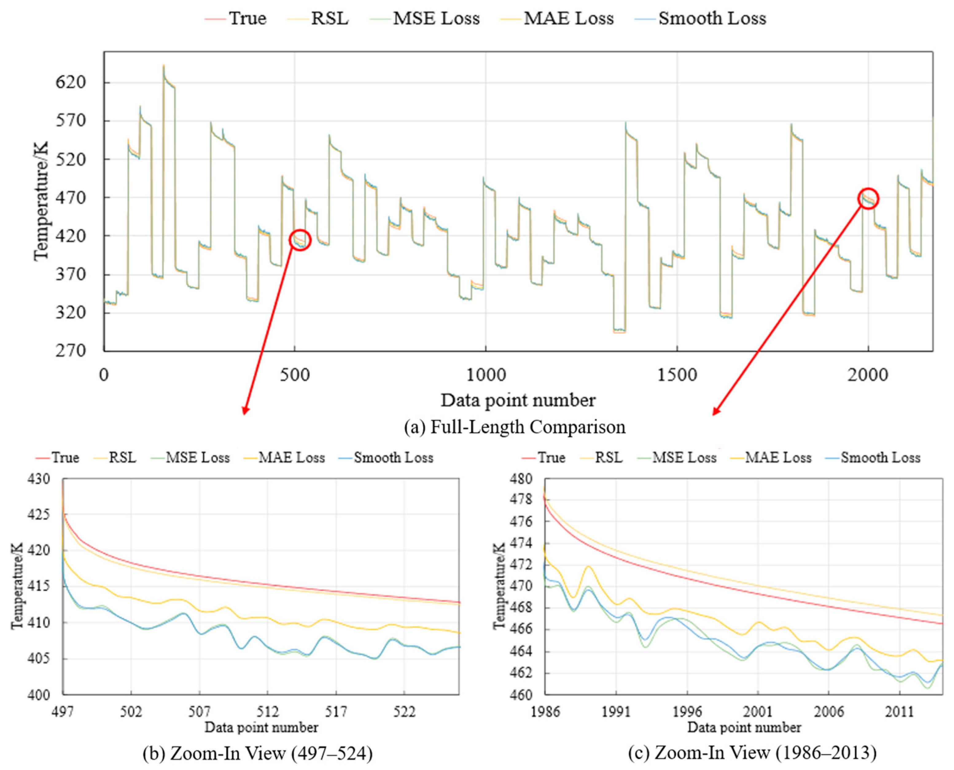
To more effectively highlight the advantages of the RSL, the prediction plot using LSTM based on different loss functions is shown in Figure 11, where the MAE of RSL using LSTM is 0.29 K, which is a significant improvement compared to the MAE of 1.77 K in the literature [11].

The LSTM model utilizing the RSL produces a prediction curve that closely approximates and, in many instances, nearly coincides with the actual data values, exhibiting an exceptional smoothness. Conversely, the prediction curves of LSTM employing traditional loss function are characterized by unsmooth and substantial discrepancies relative to the true values. This observation strongly suggests that the LSTM model equipped with RSL yields predictions of higher accuracy and robustness for this specific dataset. RSL is more suitable for dealing with the specific features and noise structure of this dataset and is more resistant to the effects of outliers.

6.4. Stability Experiments

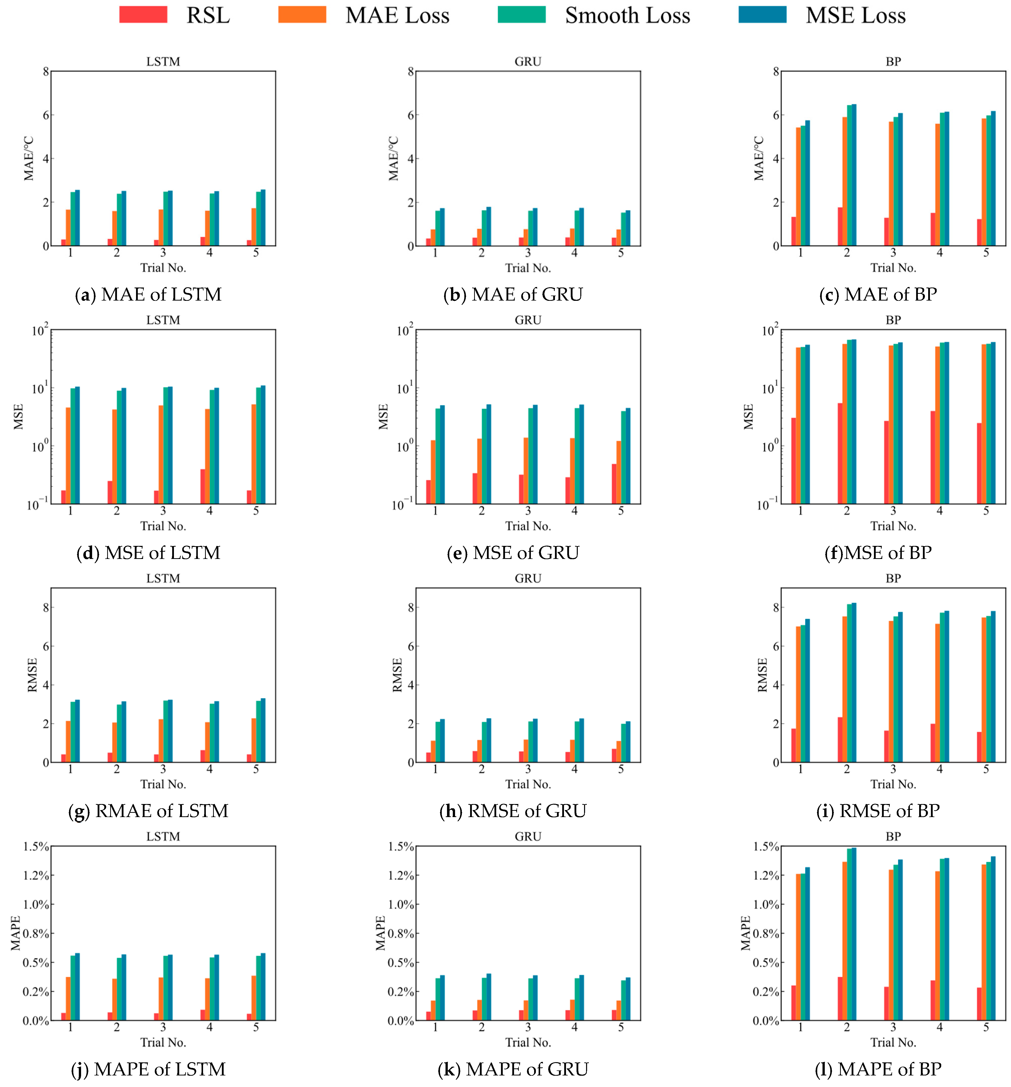
Given the inherent stochastic nature of neural network training, which encompasses aspects such as weight initialization, regularization techniques, and optimization strategies, the results vary from run to run. To assess the stability of the RSL, a series of experiments were conducted utilizing four distinct loss functions across three different models, with consistency in experimental conditions ensured through the application of identical random seeds for each trial.

Figure 12 compares the prediction curves (obtained by performing data prediction using four different loss functions) and the actual curve, derived from the four distinct loss functions and marked with different colors. In the figure, the upper subfigure displays the prediction curves for sampling points 0 to 2200, while the lower subfigure is a partial magnification of the upper one. Specifically, the left part of the lower subfigure presents the prediction curves for sampling points between 497 and 524, and the right part of the lower subfigure shows the prediction curves for sampling points between 1986 and 2013. The corresponding relationship between the upper and lower subfigure is indicated with red arrows.

Analysis of the results, as depicted in Figure 13, reveals that, across five separate trials, models employing the RSL consistently outperformed those utilizing three traditional loss functions across all evaluated metrics—MAE, MSE, RMSE, and MAPE. Consequently, this evidence suggests the superior stability of RSL over conventional alternatives.

7. Conclusions

To accurately predict the pre-insertion resistor temperature, this study proposes the integration of deep learning models with the novel rational smoothing loss function, complemented by the coati optimization algorithm and Ornstein–Uhlenbeck mutation strategy, which has been demonstrated to efficaciously predict the temperature of PIRs. This prediction capability facilitates the optimization of cooling times, thereby mitigating the risk of thermal explosion and providing crucial technical support for the secure and reliable operation of electrical transmission systems. The following key insights were derived from the research:

(1)

Compared to traditional loss functions, the rational smoothing loss function introduces an adaptive gradient adjustment for error correction, incorporating a regularization term that curtails overfitting.

(2)

The synergistic application of the coati optimization algorithm with the Ornstein–Uhlenbeck variation strategy enhances the convergence speed and parameter search efficacy, proving indispensable for the identification of optimal rational smoothing loss parameters. This combination proves instrumental in the accurate prediction of pre-insertion resistor temperature.

(3)

In comparison to traditional loss functions, the rational smoothing loss after finding parameters using the improved coati optimization algorithm significantly augments the temperature prediction accuracy of models like long short-term memory, gated recurrent unit, and backpropagation. The performance enhancements are quantified by average reduction rates of 77.97%, 93.72%, 76.59%, and 78.27% across mean absolute error, mean square error, root mean square error, and mean absolute percentage error metrics, respectively, with mean absolute error values diminishing to as low as 0.29 K. This underscores the rational smoothing loss’s potential to refine model performance, thereby elevating the precision and stability of predictions. The implementation of rational smoothing loss yields a smoother prediction curve, indicative of the model’s enhanced resistance to overfitting. This characteristic significantly boosts the model’s reliability and stability in practical deployments.

Currently, this paper presents an accurate prediction on the simulation dataset, and in the future, the proposed method can be used on an actual circuit breaker dataset in order to monitor the pre-insertion resistor temperature in real time to ensure the safe operation of the power grid.

References

1. Liu, T.; Yan, T.; Bu, X.; Duan, X.Y.; Liao, M.F. Research on phase-controlled technology of inrush current based on closing resistance. High Volt. Appar. 2018, 54, 109–114. [Google Scholar] [CrossRef]
2. Liu, P.; Liu, P.; Huang, S.; Li, G. Research of synthetic test method of capacitive current switching test for UHV circuit breaker. High Volt. Appar. 2014, 50, 87–92+98. [Google Scholar]
3. Dai, H.; Mo, S.; Wang, H.; Yin, N.; Fan, S.; Li, B. Pre-insertion resistors temperature prediction based on improved WOA-SVR. IET Sci. Meas. Technol. 2024, 18, 182–192. [Google Scholar] [CrossRef]
4. Heiermeier, H.; Raysaha, R.B. Power testing of preinsertion resistors: Limitations and solution. IEEE Trans. Power Deliv. 2016, 32, 1688–1695. [Google Scholar] [CrossRef]
5. Sun, R.; McVey, M.; Yang, D.; Stage, J.R. A study of synchronous breaker switching with preinsertion resistor for capacitors banks. IEEE Trans. Power Deliv. 2017, 33, 821–829. [Google Scholar] [CrossRef]
6. Bhatt, K.A.; Bhalja, B.R.; Parikh, U. Evaluation of controlled energization of shunt reactors for minimizing asymmetric DC component of charging current with circuit breaker having pre-insertion resistors. Int. J. Electr. Power Energy Syst. 2017, 93, 340–351. [Google Scholar] [CrossRef]
7. Gadotti, F.R.; Cabral, S.H.; Schuartz, F.M. Study of deployment of Pre-Insertion resistor to disconnector for mitigating overvoltage on 525 kV current transformers. Int. J. Electr. Power Energy Syst. 2024, 156, 109760. [Google Scholar] [CrossRef]
8. Zondi, S.; Bokoro, P.; Paul, B. EMTP-based analysis of pre-insertion resistor and point on wave switching methodology. In Proceedings of the AFRICON 2015, Addis Ababa, Ethiopia, 14–17 September 2015; pp. 1–5. [Google Scholar] [CrossRef]
9. He, L. Effects of pre-insertion resistor on energization of MMC-HVDC stations. In Proceedings of the 2017 IEEE Power & Energy Society General Meeting, Chicago, IL, USA, 16–20 July 2017; pp. 1–5. [Google Scholar] [CrossRef]
10. Da Silva, F.F.; Bak, C.L.; Guomundsdottir, U.S.; Wiechowski, W.; Knardrupgard, M.R. Use of a pre-insertion resistor to minimize zero-missing phenomenon and switching overvoltages. In Proceedings of the 2009 IEEE Power & Energy Society General Meeting, Calgary, AB, Canada, 26–30 July 2009. [Google Scholar] [CrossRef]
11. Shi, H.; Wang, Y.; Liu, Q.; Wu, C.; Chen, X.; Deng, J. Research on the fault diagnosis of pre-insertion resistor of AC filter circuit breakers. In Proceedings of the 2022 IEEE 5th International Conference on Automation, Electronics and Electrical Engineering (AUTEEE), Shenyang, China, 18–20 November 2022. [Google Scholar] [CrossRef]
12. Bao, Y.; Liu, K.; Wen, D.; Li, Y.; Wang, H.; Zhang, H. Electrical-thermal coupling characteristics of pre-insertion resistors in AC filter circuit breaker for UHV grid. Math. Biosci. Eng. 2023, 20, 12056–12075. [Google Scholar] [CrossRef]
13. Saravanan, B.; Kumar, M.D.P.; Vengateson, A. Benchmarking Traditional Machine Learning and Deep Learning Techniques for Power Transformer Fault Classification. arXiv 2025, arXiv:2505.06295. [Google Scholar] [CrossRef]
14. Box, G.E.; Jenkins, G.M.; Reinsel, G.C.; Ljung, G.M. Time Series Analysis: Forecasting and Control; Holden Bay: San Francisco, CA, USA, 1976. [Google Scholar] [CrossRef]
15. Hearst, M.A.; Dumais, S.T.; Osuna, E.; Platt, J.; Scholkopf, B. Support vector machines. IEEE Intell. Syst. Their Appl. 1998, 13, 18–28. [Google Scholar] [CrossRef]
16. Chen, T.; He, T.; Benesty, M.; Khotilovich, V.; Tang, Y.; Cho, H.; Chen, K.; Mitchell, R.; Cano, I.; Zhou, T. Xgboost: Extreme gradient boosting. R Package Version 0.4-2 2015, 1, 1–4. [Google Scholar] [CrossRef]
17. Zhu, Q. Research on fault prediction and diagnosis method of high voltage power substation equipment based on machine learning. Instrum. Meters Users 2024, 31, 24–26. [Google Scholar] [CrossRef]
18. Ijaz, M.; Jamil, M.S.; Ali, S.; Ghazali, R.R.; El-Saoud, W.A. A novel AI-based power flow controller for distributed energy resources. Energy Rep. 2021, 7, 5281–5290. [Google Scholar] [CrossRef]
19. Graves, A. Long short-term memory. In Supervised Sequence Labelling with Recurrent Neural Networks; Springer: Berlin/Heidelberg, Germany, 2012; pp. 37–45. [Google Scholar]
20. Dey, R.; Salem, F.M. Gate-variants of gated recurrent unit (GRU) neural networks. In Proceedings of the 2017 IEEE 60th International Midwest Symposium on Circuits and Systems (MWSCAS), Boston, MA, USA, 6–9 August 2017; pp. 1597–1600. [Google Scholar] [CrossRef]
21. Medsker, L.R.; Jain, L. Recurrent neural networks. Des. Appl. 2001, 5, 2. [Google Scholar]
22. Chen, Q.; Cai, C.; Chen, Y.; Zhou, X.; Zhang, D.; Peng, Y. TemproNet: A transformer-based deep learning model for seawater temperature prediction. Ocean Eng. 2024, 293, 116651. [Google Scholar] [CrossRef]
23. Jun, J.; Kim, H.K. Informer-Based Temperature Prediction Using Observed and Numerical Weather Prediction Data. Sensors 2023, 23, 7047. [Google Scholar] [CrossRef]
24. Pal, S.K.; Mitra, S. Multilayer perceptron, fuzzy sets, and classification. IEEE Trans. Neural Netw. 1992, 3, 683–697. [Google Scholar] [CrossRef]
25. Zeng, A.; Chen, M.; Zhang, L.; Xu, Q. Are transformers effective for time series forecasting? AAAI Conf. Artif. Intell. 2023, 37, 11121–11128. [Google Scholar] [CrossRef]
26. Yi, K.; Zhang, Q.; Fan, W.; Wang, S.; Wang, P.; He, H.; An, N.; Lian, D.; Cao, L.; Niu, Z. Frequency-domain MLPs are more effective learners in time series forecasting. Adv. Neural Inf. Process. Syst. 2024, 36, 76656–76679. [Google Scholar] [CrossRef]
27. LeCun, Y.; Bengio, Y. Convolutional networks for images, speech, and time series. In The Handbook of Brain Theory and Neural Networks; Arbib, M.A., Ed.; MIT Press: Cambridge, MA, USA, 1995; pp. 255–258. [Google Scholar] [CrossRef]
28. Imani, M. Electrical load-temperature CNN for residential load forecasting. Energy 2021, 227, 120480. [Google Scholar] [CrossRef]
29. Zhang, Z.; Dong, Y. Temperature forecasting via convolutional recurrent neural networks based on time-series data. Complexity 2020, 2020, 3536572. [Google Scholar] [CrossRef]
30. Wang, H.; Peng, J.; Huang, F.; Wang, J.; Chen, J.; Xiao, Y. Micn: Multi-scale local and global context modeling for long-term series forecasting. In Proceedings of the Eleventh International Conference on Learning Representations (ICLR), Virtual, 1–5 May 2023. [Google Scholar] [CrossRef]
31. Wu, H.; Hu, T.; Liu, Y.; Zhou, H.; Wang, J.; Long, M. TimesNet: Temporal 2D-variation modeling for general time series analysis. arXiv 2022, arXiv:2210.02186. [Google Scholar] [CrossRef]
32. Bao, Y.; Liu, K.; Wu, Y.; Chen, B.; Yao, Y.; Wang, R. Analysis of influence of porosity on electric field and temperature in pre-insertion resistors. In Proceedings of the Fourth International Conference on Testing Technology and Automation Engineering (TTAE 2024), Xiamen, China, 6–8 September 2024; Volume 13439. [Google Scholar] [CrossRef]
33. Chen, X.; Yu, R.; Ullah, S.; Wu, D.; Li, Z.; Li, Q.; Qi, H.; Liu, J.; Liu, M.; Zhang, Y. A novel loss function of deep learning in wind speed forecasting. Energy 2022, 238, 121808. [Google Scholar] [CrossRef]
34. Wang, H.; Li, B.; Fan, S.; Wu, Y.; Liu, X. TimeSQL: Improving multivariate time series forecasting with multi-scale patching and smooth quadratic loss. Inf. Sci. 2024, 671, 120652. [Google Scholar] [CrossRef]
35. Maclaurin, C. A Treatise of Fluxions: In Two Books; T. W. and T. Ruddimans: Edinburgh, UK, 1742. [Google Scholar]
36. Taylor, B. Methodus Incrementorum Directa & Inversa; William Innys: London, UK, 1717. [Google Scholar]
37. Dehghani, M.; Montazeri, Z.; Trojovská, E.; Trojovský, P. Coati Optimization Algorithm: A new bio-inspired metaheuristic algorithm for solving optimization problems. Knowl.-Based Syst. 2023, 259, 110011. [Google Scholar] [CrossRef]
38. Pappula, L.; Ghosh, D. Cat swarm optimization with normal mutation for fast convergence of multimodal functions. Appl. Soft Comput. 2018, 66, 473–491. [Google Scholar] [CrossRef]
39. Shan, W.; He, X.; Liu, H.; Heidari, A.A.; Wang, M.; Cai, Z.; Chen, H. Cauchy mutation boosted Harris hawk algorithm: Optimal performance design and engineering applications. J. Comput. Des. Eng. 2023, 10, 503–526. [Google Scholar] [CrossRef]
40. Li, Q.; Zeng, X.; Wei, W. Multi-objective particle swarm optimization algorithm using Cauchy mutation and improved crowding distance. Int. J. Intell. Comput. Cybern. 2023, 16, 250–276. [Google Scholar] [CrossRef]
41. Rajesh, P.; Shajin, F.H. Optimal allocation of EV charging spots and capacitors in distribution network improving voltage and power loss by Quantum-Behaved and Gaussian Mutational Dragonfly Algorithm (QGDA). Electr. Power Syst. Res. 2021, 194, 107049. [Google Scholar] [CrossRef]
42. Bo, N.; Feiyue, M.; Pei, D. Fault analysis of pre-insertion resistors for 800 kV circuit breakers in AC filters field. High Volt. Appar. 2020, 56, 36–43. [Google Scholar] [CrossRef]
43. Shi, C.; Chen, S.; Wang, Y.; Jin, S.; Yu, Y.; He, Y.; Yang, S.; Xiong, Z.; Shi, Q. Effects of fibre orientation on thermal conductivity of epoxy/glass fibre composites. Eng. Plast. Appl. 2022, 50, 108–116. [Google Scholar] [CrossRef]
44. Zhang, Y.; Du, C.; Shi, M.; Wang, Z. Summary of solid insulating materials for high volt-age switchgear. Electr. Eng. Mater. 2022, 182, 65–67. [Google Scholar] [CrossRef]
Figure 1. RPL, MAE loss, MSE loss, and their derivatives.
Energies 18 05484 g001
Figure 2. Ornstein–Uhlenbeck process.
Energies 18 05484 g002
Figure 3. Convergence curve of the test function.
Energies 18 05484 g003
Figure 4. The circuit diagram of the circuit break.
Energies 18 05484 g004
Figure 5. Simulation model.
Energies 18 05484 g005
Figure 6. Single-chip PIR.
Energies 18 05484 g006
Figure 7. Relationship between multiple physical fields.
Energies 18 05484 g007
Figure 8. Current wave and parameters of PIR.
Energies 18 05484 g008aEnergies 18 05484 g008b
Figure 9. Results for different meshes.
Energies 18 05484 g009
Figure 10. Results with different step sizes.
Energies 18 05484 g010
Figure 11. Heat capacity experiment (cooling, 900 s).
Energies 18 05484 g011
Figure 12. Forecast curve.
Energies 18 05484 g012
Figure 13. Stability experiments of four loss functions.
Energies 18 05484 g013