Abstract
Managing electric vehicle (EV) charging at stations with on-site solar (PV) generation is a complex task, made difficult by volatile electricity prices and the need to guarantee services for drivers. This paper proposes a robust optimization (RO) framework to schedule EV charging, minimizing electricity costs while explicitly hedging against price uncertainty. The model is formulated as a tractable linear program (LP) using the Bertsimas–Sim reformulation and is implemented in an online, adaptive manner through a model predictive control (MPC) scheme. Evaluated on extensive real-world charging data, the proposed controller demonstrates significant cost reductions, outperforming a PV-aware Greedy heuristic by 17.5% and a deep reinforcement learning (DRL) agent by 12.2%. Furthermore, the framework exhibits lower cost volatility and is proven to be computationally efficient, with solving times under five seconds even during peak loads, confirming its feasibility for real-time deployment. The results validate our framework as a practical, reliable, and economically superior solution for the operational management of modern EV charging infrastructure.
1. Introduction
Climate change remains a defining challenge of this century. Vietnam’s commitment to net-zero by 2050 [1] reflects a decisive policy stance, yet the pathway requires the major decarbonization of transport—a sector responsible for roughly 10.8% of national emissions and projected to grow 6–7% annually [2]. Accelerating the uptake of electric vehicles (EVs) is therefore pivotal [3]. Domestic momentum—illustrated by rapid EV market growth [4,5]—exposes infrastructure bottlenecks: public charging scarcity [6], stressed urban feeders, and rising operating costs. Given Vietnam’s strong solar resource, co-locating PVs at charging stations is a promising lever to reduce grid imports, hedge prices, and advance net-zero goals [7].
1.1. Positioning Within Recent Literature
PV-coupled EV charging has matured along four complementary strands. (i) Planning and siting with renewables: system-level studies co-optimize the siting/sizing of charging infrastructure and renewables within grid limits, but do not address real-time station operations [8]. (ii) Station-level operational control (MPC): large facilities with PV and hundreds of chargers deploy model predictive control using forecasts to balance building limits and service quality, typically under deterministic or point-forecasted prices [9]. (iii) Uncertainty-aware scheduling and robust optimization: newer works build stochastic or robust formulations to protect against price/load/solar errors—e.g., robust dispatch with EV aggregators and studies of uncertain charging flexibility [10,11]. These approaches improve worst-case behavior but often rely on large scenario sets or complex uncertainty sets. (iv) PV-aware smart charging at stations: surveys of integrated EVCS–PV–ESS architectures synthesize capacity allocation and control strategies aimed at improving self-consumption and reducing curtailment [12,13]. Related but orthogonal to our focus, resilience-oriented planning leverages mobile robot chargers to sustain service under extreme conditions [14].
1.2. Gap and Contributions
This paper targets the under-explored intersection of station-level scheduling with on-site PV and explicit protection against day-ahead price errors, while keeping the controller lightweight. Unlike planning papers that decide siting/sizing [8], we assume an existing site; unlike deterministic MPC [9], we do not rely on accurate prices; and unlike scenario-heavy stochastic control [10,11], we avoid large ensembles by adopting a budgeted (Bertsimas–Sim) price-uncertainty model that integrates directly into a linear program (LP). Concretely, our contributions are given as follows:
- Robust PV-coupled station optimizer. We formulate a linear program that co-schedules per-EV charging and PV utilization under a budgeted electricity-price uncertainty set, yielding a single tunable parameter to trade nominal cost for worst- case protection.
- Scenario-free MPC integration. We embed the robust LP in a receding-horizon loop that re-solves on arrivals/departures or at fixed intervals, maintaining computational tractability for large stations without scenario generation.
- Empirical evaluation on realistic data. Using real prices, irradiance, and multi-EV session traces, we quantify nominal savings, robustness benefits, and solve-time scaling versus a baseline scheduler.
1.3. Paper Organization
2. Symbols and Parameters
The parameters used in the optimization model are defined below:
- T: Number of time steps in a day (e.g., h).
- : Length of each time step (hours).
- N: Number of electric vehicles (EVs).
- : Electricity price from the grid at time t (Euro/kWh).
- : Solar energy output at time t (kW).
- : Maximum achievable solar energy output at time t (kW).
- : Maximum charging power provided by the charging station for EV i (kW).
- : Matrix representing the charging time of vehicle i by hour.
- : Grid capacity limit (kW).
- : Charging efficiency of the EV (in the range ).
- : Minimum required energy (kWh) that the EV i needs when leaving the station.
- : Set of time points when EV i is present at the station (based on ).
3. Optimization Model
Several straightforward solutions have been considered for managing EV charging, such as the “First Come, First Served” (FCFS) principle, which guarantees equity by servicing vehicles in the sequence of their arrival. However, FCFS lacks consideration of critical factors such as electricity pricing, real-time energy demand, and overall impact on the power grid. This limitation can lead to inefficient energy allocation, increased operational costs, and potential grid instability, especially during peak demand periods.
Figure 1 illustrates the power flow diagram of charging stations with solar-integration. The charging socket receives energy from both the solar panel and the grid, and then delivers it to the EVs. In this model, we employ a linear programming approach to minimize net electricity consumption costs, which only occur when the charging demand exceeds the available solar renewable energy.

Figure 1.
On-site solar-integrated charging station model.
Decision variables:
- : Charging power (kW) of EV i at time t.
- : Auxiliary variable representing the positive part of the net load at time t, that is
- : The amount of solar energy used at time t.
Objective Function:
where is used to linearize the expression .
The solar contribution is computed as follows:
where
- indicates the area of the PV panels in m2;
- indicates the solar irradiance in W/m2;
- is the efficiency of the PV panels.
Constraints:
- Each EV i must be charged with at least the minimum required energy throughout its available period . Here, is the charging efficiency, is the charging power at time t, and is the length of each time interval. This requirement can be expressed as
- The charging power of each EV at time t must not exceed the maximum power limit that the station provides. However, the actual available power is scaled by the fraction of the time interval during which the EV i is connected, denoted by . For example, if the EV is connected only for 10 min in an hour (i.e., ), then the maximum available charging power becomes . When the EV is not connected (i.e., ), no charging power is provided, ensuring that . This is modelled by
- The total charging power from all EVs at time t must not exceed the maximum grid capacity after subtracting the renewable energy :
- The variable represents the additional power to be purchased from the grid if the total charging power exceeds . When renewable energy sufficiently supplies the EVs, may be zero. It is ensured that the power purchased from the grid cannot be negative:
- Finally, the solar energy cannot exceed its maximum available limit at each time and it must be greater than or equal to 0:
Database:
We obtained detailed charging session information from 2018 to 2019 from ACN Data—a public dataset on electric vehicle (EV) charging collected through a collaboration between the PowerFlex System and the California Institute of Technology (Caltech) [15]. This dataset comprises detailed information on EV charging sessions at two distinct locations: the Caltech campus and the Jet Propulsion Laboratory (JPL) campus. The JPL site is representative of workplace charging, whereas Caltech represents a hybrid of workplace and public charging.
We selected hourly electricity price data for Spain corresponding to the same period as the charging data, sourced from Ember—European Wholesale Electricity Price Data [16].
Hourly irradiance data were obtained from the EU Science Hub [17] for the same period. We assume that represents [W/m2]—the global in-plane irradiance with a slope of and an azimuth of —with Madrid, Spain, chosen as the representative location.
Lastly, Table 1 shows the values of the constant parameters used during the simulation.

Table 1.
Constant values used in the simulation.
4. Proposed Methodology
To account for uncertainty in the electricity price, we model the grid price at time t as
where is the nominal electricity price and represents the deviation from this nominal value. We assume that the deviation is bounded as
To avoid an overly conservative solution—i.e., assuming that every time period experiences the maximum deviation simultaneously—we adopt a budget of uncertainty . The uncertainty set for is defined as
The nominal electricity cost from the grid is given by
where represents the purchased electricity (in kW) from the grid at time t. Under uncertainty, the robust counterpart of the objective becomes a min–max formulation:
This expression can be decomposed into the nominal cost and the additional cost resulting from the uncertainty:
4.1. Bertsimas–Sim Reformulation
We now reformulate the inner maximization problem:
subject to
Here, the terms and are treated as fixed parameters. Following the approach of Bertsimas and Sim [18], we introduce an auxiliary scalar variable and auxiliary variables for all . The worst-case additional cost due to price deviation is then equivalently expressed as
subject to the dual feasibility constraints
4.2. Final Robust Optimization Model
Incorporating the Bertsimas–Sim reformulation into the full model, the robust optimization problem is given by
Here, the term represents the nominal electricity cost from the grid, while captures the worst-case additional cost under bounded price uncertainty. The budget parameter offers a flexible trade-off between protection against extreme scenarios and conservatism in scheduling decisions.
4.3. Algorithm Development: An Online Implementation
The robust optimization model presented in the previous sections addresses the power allocation problem in a static (offline) setting, assuming that all information about charging sessions is known beforehand. However, in a real-world operational environment, charging stations must operate dynamically (online), handling the random and continuous arrival and departure of electric vehicles. To address this challenge, we develop an online control algorithm based on the Model Predictive Control (MPC) methodology.
The MPC approach allows our optimization model to be applied in real-time. The core idea is that, at each time step, the algorithm solves an optimization problem for a future prediction horizon but only executes the control action for the immediate next time step. This process is repeated, enabling the system to continuously update and adapt to new information. The specific algorithm is presented in Algorithm 1.
| Algorithm 1 Online smart charging using MPC |
|
The algorithm operates in a continuous loop over time slots k. At each slot, it performs the following steps:
- Handling new arrivals (Lines 4–6): When a new electric vehicle j connects to the station at time k, the system initializes and records its remaining energy demand, , to be its total required energy .
- Re-optimization trigger (Line 8): Instead of re-solving the optimization problem at every time slot (which is computationally expensive), we use a dual-trigger mechanism. The optimization process is invoked only when one of the following two conditions is met:
- Event-driven trigger: A new vehicle arrives or an existing one departs. This ensures that the system reacts immediately to changes in charging demand.
- Time-driven trigger: A predefined time interval has passed since the last optimization (). This ensures that the charging schedule is periodically updated to reflect the changes in external factors, such as the electricity price or the expected solar energy generation.
- Solving the optimization problem (Lines 9–11): When triggered, the algorithm will
- Determine the set of vehicles currently at the station that still require charging ().
- Establish a prediction horizon T, starting from the current time k, and extending to the latest departure time among all vehicles in .
- Call the function OPT(), which is the robust optimization model, to find the optimal charging schedule and solar energy usage plan for the entire horizon T.
- Execution and state update (Lines 13–17): This step embodies the MPC principle. Instead of applying the entire calculated schedule , the algorithm only executes the first step of the plan:
- It assigns the charging power for each vehicle i and the solar energy usage only for the current time slot k.
- It then updates the system’s state by reducing the remaining energy demand of each vehicle based on the actual energy delivered in that time slot ().
By repeating this cycle, the algorithm enables the charging station to continuously optimize its operations dynamically, ensuring cost-effectiveness while adapting to the unpredictable nature of real-world EV charging sessions.
5. Results and Discussion
5.1. Experimental Setup and Baselines
We evaluate the proposed robust LP controller in a receding-horizon loop against three baselines that reflect common practice and stronger algorithmic alternatives:
- FCFS (first come, first served). Power is allocated according to arrival order without considering real-time prices. At time t, the power to EV i is , where is the connector limit, is the remaining energy of EV i, and is the station’s remaining capacity. If , subsequent arrivals must wait.
- Greedy price-first (PV-aware). A myopic heuristic that uses all available PV first, then fills the residual demand with grid energy starting from the lowest-price slots subject to per-connector and station limits. Implementation details are provided in as shown in Algorithm A1 in Appendix A.
- DRL (DQN) Baseline. A Deep Q-Network policy that, at each slot, chooses binary per-EV grid on/off decisions while PV is allocated greedily. The state aggregates price, PV, grid capacity, and session features; the reward is the negative electricity cost with penalties for unmet energy at departure. Training and update rules appear in as shown in Appendix B.
All methods are evaluated on the same arrivals/departures, PV profiles, price signals, and physical limits. Unless otherwise specified, the robustness budget in our controller is fixed across months.
5.2. Monthly Cost Comparison
Figure 2 reports monthly electricity costs from 25 April 2018 to 31 December 2019 for the three methods. The proposed LP attains the lowest cost in every month, outperforming both Greedy price-first and DRL (DQN). Over the entire horizon, the LP reduces total cost by 17.5% relative to Greedy and by 12.2% relative to DQN, with typical monthly savings of EUR 233 and EUR 153, respectively. Improvements are pronounced in shoulder/winter periods when PV is scarce, indicating more effective price-aware scheduling. Late-summer 2018 shows the highest absolute costs across all methods, but the LP still maintains a consistent advantage.
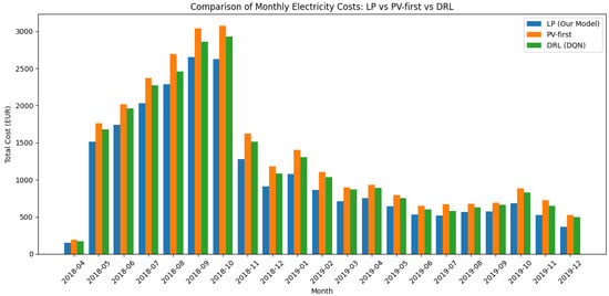
Figure 2.
Monthly electricity costs for LP (ours), Greedy price-first, and DRL (DQN) from 2018 to 04 to 2019-12.
5.3. Weekly Cost Distribution
To examine distributional properties, Figure 3 shows weekly cost box plots for the same period. The LP exhibits the lowest median and a visibly narrower interquartile range (IQR) than both baselines, demonstrating lower volatility week-to-week. The upper whisker is also shorter for the LP, indicating fewer extreme high-cost weeks. These distributional results complement the monthly aggregates by showing that the LP improves both the central tendency and the tail behavior of operating costs.
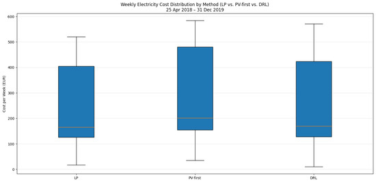
Figure 3.
Weekly cost distribution for LP (ours), Greedy price-first, and DRL (DQN) from 2018-04 to 2019-12.
5.4. Comparing Total Power Allocation Based on Price Fluctuation
The temporal allocation patterns explain the observed savings. The panels in Figure 4 compare total charging power across a representative day under varying prices. The LP concentrates charging in low-price valleys and throttles during peaks, while non-price-aware allocation (e.g., FCFS) often consumes grid energy during expensive hours, driving up costs. For example, at Caltech, around 02:00 on 7 September 2018 (price EUR/MWh), the LP schedules substantially more energy than FCFS; the latter compensates later at higher prices, resulting in unnecessary expenditure. Similar dynamics appear at JPL around 00:00 on 2 May 2019. Overnight charging windows are particularly advantageous for the LP due to sustained low prices.
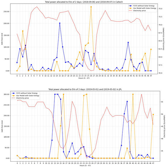
Figure 4.
Comparing total power allocation based on price fluctuation.
5.5. Additional Observations
The analysis is consistent with site-specific comparisons against FCFS using the ACN data: at Caltech (25,981 sessions), cost reductions ranged from ∼10 to 14% in early months to larger gains in periods with pronounced price spikes; at JPL (22,185 sessions), savings ranged from ∼6.2% to ∼19.2%. A marked decline in charging activity after 1 November 2018 at Caltech corresponds to a tariff change (introduction of a 0.12 USD/kWh fee), which reduces demand and lowers absolute costs for all methods while preserving the LP’s relative advantage.
5.6. Sensitivity Analysis on the Robustness Parameter
The budget of uncertainty, , is a critical parameter that allows the decision maker to control the trade-off between the nominal cost and the level of protection against price volatility. A value of corresponds to the nominal, non-robust optimization, where price uncertainty is ignored. As increases, the solution becomes more conservative, protecting against worst-case price deviations across a larger number of time periods.
To analyze this trade-off, we performed a lightweight sensitivity analysis on a representative one-week period from the Caltech dataset, which includes 215 charging sessions. We ran our optimization model with three distinct values for : 0 (nominal), 15 (moderate), and 30 (conservative). The results, summarized in Table 2, illustrate the “price of robustness.”
Table 2.
Sensitivity analysis of total cost for a representative week with varying .
As shown in Table 2, increasing from 0 to 30 leads to a modest 4.64% increase in the planned nominal cost. This increase represents the premium paid to safeguard against uncertainty. In return, the worst-case cost—the maximum potential cost under the most adverse price fluctuations allowed by the uncertainty set—is significantly reduced by approximately 14%. This demonstrates the effectiveness of the robust optimization framework: for a small, predictable increase in the base operational cost, the model provides substantial protection against unforeseen price spikes, thereby reducing financial risk for the charging station operator.
5.7. Computational Performance
For the proposed online scheduling framework to be practical, the optimization problem must be solvable within a reasonable timeframe. We evaluated the computational performance of our MPC algorithm (Algorithm 1) on a standard laptop (Intel Core i7, 16 GB RAM) using Python 3.12.2 with the Gurobi solver. The primary factor influencing the solving time is the number of active EVs () at the station. Table 3 reports the average time required to solve the optimization problem for varying the numbers of concurrent EVs.
Table 3.
Average solve time per optimization instance.
The results indicate that the model is computationally efficient. Even under peak load conditions with 50 concurrent EVs, the optimization problem is solved in under 5 s. This runtime is well within the practical limits for an online system where re-optimization may be triggered every 5–15 min or upon a new event. The performance demonstrates that the proposed framework is not only theoretically sound but also computationally feasible for real-world deployment.
6. Limitations and Future Work
While the proposed robust optimization framework demonstrates significant cost savings and computational efficiency, several limitations present opportunities for future research:
- Modeling of uncertainty: The current model robustly handles uncertainty in electricity prices but treats other key variables as deterministic. A primary area for extension is to incorporate uncertainty in solar (PV) generation forecasts and EV behavior, such as unexpected early departures or changes in energy demand. Methodologies like stochastic programming or more advanced distributionally robust optimization (DRO) could be employed to create a more comprehensive model that accounts for these multiple sources of uncertainty.
- Scope of objectives: The optimization objective is focused solely on minimizing the direct operational electricity cost. Future work could explore a multi-objective framework that balances cost with other important goals. These could include minimizing battery degradation for EVs, maximizing user satisfaction, or providing ancillary services to the grid.
- System boundaries: The model optimizes the operation of a single charging station. An important research direction is to extend this framework to a network of charging stations, considering grid-level constraints and coordinated charging strategies.
- Comparison with advanced learning methods: While the LP model outperformed the DQN baseline, future research could involve benchmarking against more sophisticated deep reinforcement learning (DRL) agents using continuous action spaces (e.g., soft actor–critic, SAC).
7. Conclusions
This paper presents a robust optimization framework for scheduling EV charging at stations with on-site solar generation, specifically designed to mitigate financial risks from electricity price volatility. By leveraging the Bertsimas–Sim reformulation, we developed a tractable linear programming model solved within a model predictive control loop, enabling practical, online implementation.
Our simulation results, based on real-world data, confirm the effectiveness of our approach. The proposed controller consistently outperforms common industry practices and learning-based alternatives, achieving average total cost reductions of 17.5% compared to a PV-aware Greedy heuristic and 12.2% compared to a DRL agent. Our method also demonstrates superior performance in reducing cost volatility.
Furthermore, the framework’s practicality is validated through sensitivity and computational analyses. The model offers a flexible trade-off between cost and risk protection and is computationally efficient enough for real-time deployment, solving complex problems in under five seconds. In summary, this work delivers a tractable, economically advantageous, and risk-aware solution for managing modern EV charging infrastructure.
Author Contributions
Conceptualization, A.N. and C.D.; methodology, A.N.; software, H.P.; validation, A.N., H.P. and C.D.; formal analysis, A.N.; investigation, H.P.; resources, C.D.; data curation, H.P.; writing—original draft preparation, A.N. and H.P.; writing—review and editing, C.D.; visualization, A.N.; supervision, C.D.; project administration, C.D. All authors have read and agreed to the published version of the manuscript.
Funding
This research received no external funding.
Institutional Review Board Statement
Not applicable.
Informed Consent Statement
Not applicable.
Data Availability Statement
The data used in this study are publicly available. ACN-Data can be found at https://ev.caltech.edu/dataset (accessed on 18 March 2025), European electricity price data at https://ember-energy.org/data/european-wholesale-electricity-price-data/ (accessed on 18 March 2025), and solar irradiance data at https://joint-research-centre.ec.europa.eu/photovoltaic-geographical-information-system-pvgis/pvgis-tools/hourly-radiation_en (accessed on 18 March 2025).
Acknowledgments
The authors would like to acknowledge the providers of the open source datasets used in this research.
Conflicts of Interest
The authors declare no conflicts of interest.
Appendix A. Greedy PV-First Heuristic
Appendix A.1. Description
The Greedy PV-first algorithm serves as a simple, non-price-aware baseline. Its policy is to maximize the use of available solar (PV) energy at every time step. Specifically, it allocates available PV power as evenly as possible among all connected EVs. If the PV supply is insufficient to meet their charging needs, it then draws power from the grid to fill the remaining demand, up to the station’s grid capacity limit (). This allocation strategy is myopic and completely ignores electricity price signals.
Appendix A.2. Rationale
This heuristic is included because it represents a common “renewables-first” policy that is intuitive and easy to implement in practice. It provides a useful lower bound for evaluating the economic benefits of more sophisticated, price-aware optimization strategies.
Appendix A.3. Key Characteristics
- Advantages: Fully utilizes on-site renewable generation and is computationally trivial, requiring no optimization solver.
- Limitations: Its obliviousness to electricity prices can lead to high operational costs, especially if grid power is consumed during peak price periods. It also does not account for fairness or differing urgency among EVs (e.g., imminent departure times).
| Algorithm A1 Greedy PV-first heuristic |
|
Appendix B. Deep Reinforcement Learning (DQN) Baseline
Appendix B.1. Description
This baseline uses a deep Q-network (DQN) agent to learn a charging policy. At each time step, the agent makes a binary (on/off) decision for each EV regarding whether it should receive power from the grid. Similarly to the Greedy heuristic, available PV energy is always prioritized and allocated first. The DQN’s goal is to learn a sequence of actions that minimizes total electricity costs while ensuring that all EVs are fully charged by their departure times.
Appendix B.2. Markov Decision Process (MDP) Formulation
- State (): A vector representing the system at time k, including the current electricity price (), available PV generation (), total grid capacity (), and features for each active EV (e.g., remaining energy demand, connector power limit, time until departure).
- Action (): A vector of binary decisions for each EV i, where 1 indicates enabling grid charging and 0 indicates disabling it.
- Reward (): The reward is the negative electricity cost incurred in a time step: . A large negative penalty is applied if an EV departs with unmet energy demand, encouraging the agent to prioritize service completion.
Appendix B.3. Training and Deployment
The DQN agent is trained offline using historical data (Algorithm A2). During deployment (Algorithm A3), the trained network selects the optimal action at each step based on the current state.
| Algorithm A2 DQN training for EV charging |
|
| Algorithm A3 DQN deployment (inference) |
|
Appendix B.4. Hyperparameters and Training Setup
The hyperparameters used for training the DQN agent are listed below.
| Training Episodes: 5 |
| Discount Factor (gamma): 0.98 |
| Learning Rate: 1e-3 |
| Batch Size: 128 |
| Replay Buffer Size: 50,000 |
| Epsilon Start: 0.2 |
| Epsilon End: 0.05 |
| Epsilon Decay Steps: 2000 |
| NN Hidden Dimensions: 64 |
| Unmet Demand Penalty: 1e6 |
Appendix B.5. Ablation Study: Training Budget vs. Performance
We analyzed the impact of the training budget (number of episodes) on the DQN agent’s performance. The results are summarized in Table A1.
Table A1.
Effect of the training budget on DQN performance. “Savings” are calculated relative to the Greedy PV-first baseline cost. “Deficit” refers to the total unmet energy demand at departure across all sessions.
Table A1.
Effect of the training budget on DQN performance. “Savings” are calculated relative to the Greedy PV-first baseline cost. “Deficit” refers to the total unmet energy demand at departure across all sessions.
| Episodes | Runtime | DRL Cost (EUR) | Savings (%) | Deficit (kWh) |
|---|---|---|---|---|
| 2 | 00:00:22 | 3276 | 13.23% | 2866.06 |
| 5 | 00:00:37 | 3596 | 4.75% | 894.81 |
| 10 | 00:01:00 | 3642 | 3.54% | 686.62 |
| 15 | 00:01:50 | 3753 | 0.59% | 97.87 |
| 20 | 00:02:30 | 3767 | 0.22% | 2.09 |
Interpretation
The results show a clear trade-off between cost optimization and service quality (i.e., minimizing the energy deficit). With very few training episodes, the agent learns a cost-saving policy but fails to reliably charge all vehicles. As the number of episodes increases, the large penalty for unmet demand forces the agent to prioritize service completion, significantly reducing the energy deficit to near zero. However, this comes at the cost of less aggressive price-aware scheduling, causing its economic performance to converge towards that of the simpler Greedy PV-first baseline. This suggests that achieving a better balance may require tuning the penalty term or adopting a constrained reinforcement learning formulation.
References
- Vietnam Government. Vietnam’s Commitment to Achieve Net-Zero by 2050. 2021. Available online: https://en.baochinhphu.vn/vietnam-commits-to-achieve-net-zero-emissions-by-2050-111211101190824684.htm (accessed on 17 September 2025).
- Ministry of Transport. Transport Sector Emissions and Projections. 2022. Available online: https://www.mt.gov.vn/ (accessed on 17 September 2025).
- International Energy Agency. Global EV Outlook 2023. 2023. Available online: https://www.iea.org/reports/global-ev-outlook-2023 (accessed on 17 September 2025).
- VinFast. VinFast Launches First EV Models. 2021. Available online: https://vinfastauto.com/vn_en/newsroom/press-release (accessed on 17 September 2025).
- VNExpress. VinFast Sells 51,000 EVs by 2024. 2024. Available online: https://e.vnexpress.net/news/business/vinfast-sells-51000-evs-by-2024-4728339.html (accessed on 17 September 2025).
- Vietnam Investment Review. Vietnam Faces Shortage of EV Charging Stations. 2024. Available online: https://vir.com.vn/vietnam-faces-shortage-of-ev-charging-stations-110097.html (accessed on 17 September 2025).
- RMIT. The Future Is Bright for Electric Vehicles Despite Challenges. 2024. Available online: https://www.rmit.edu.vn/news/all-news/2024/nov/the-future-is-bright-for-electric-vehicles-despite-challenges (accessed on 17 September 2025).
- Wang, B.; Dehghanian, P.; Zhao, D. Coordinated Planning of Electric Vehicle Charging Infrastructure and Renewables in Power Grids. IEEE Open Access J. Power Energy 2023, 10, 233–244. [Google Scholar] [CrossRef]
- Hermans, B.A.L.M.; Walker, S.; Ludlage, J.H.A.; Özkan, L. Model predictive control of vehicle charging stations in grid-connected microgrids: An implementation study. Appl. Energy 2024, 368, 123210. [Google Scholar] [CrossRef]
- Liu, X.; Li, Z.; Yang, X.; Li, Z.; Wei, Z.; Wang, P. Two-stage robust economic dispatch of distribution systems with electric vehicle aggregators. Electr. Power Syst. Res. 2025, 248, 111850. [Google Scholar] [CrossRef]
- Chemudupaty, R.; Bahmani, R.; Fridgen, G.; Marxen, H.; Pavić, I. Uncertain electric vehicle charging flexibility, its value on spot markets, and the impact of user behaviour. Appl. Energy 2025, 394, 126063. [Google Scholar] [CrossRef]
- Yao, M.; Li, C.; Li, C.; Li, H. A Review of Capacity Allocation and Control Strategies for Electric Vehicle Charging Stations with Integrated Photovoltaic and Energy Storage Systems. World Electr. Veh. J. 2024, 15, 101. [Google Scholar] [CrossRef]
- Qian, K.; Fachrizal, R.; Munkhammar, J.; Ebel, S.; Adam, A. Large-scale EV charging scheduling considering on-site PV generation by combining an aggregated model and sorting-based methods. Sustain. Cities Soc. 2024, 107, 105453. [Google Scholar] [CrossRef]
- An, S.; Qiu, J.; Lin, J.; Yao, Z.; Liang, Q.; Lu, X. Planning of a multi-agent mobile robot-based adaptive charging network for enhancing power system resilience under extreme conditions. Appl. Energy 2025, 395, 126252. [Google Scholar] [CrossRef]
- Caltech. ACN-Data—A Public EV Charging Dataset. 2019. Available online: https://ev.caltech.edu/dataset (accessed on 17 September 2025).
- Ember. European Wholesale Electricity Price Data. 2024. Available online: https://ember-energy.org/data/european-wholesale-electricity-price-data/ (accessed on 17 September 2025).
- EU Science Hub. Hourly Radiation. 2016. Available online: https://joint-research-centre.ec.europa.eu/photovoltaic-geographical-information-system-pvgis/pvgis-tools/hourly-radiation_en (accessed on 17 September 2025).
- Bertsimas, D.; Sim, M. The Price of Robustness. Oper. Res. 2004, 52, 35–53. [Google Scholar] [CrossRef]
Disclaimer/Publisher’s Note: The statements, opinions and data contained in all publications are solely those of the individual author(s) and contributor(s) and not of MDPI and/or the editor(s). MDPI and/or the editor(s) disclaim responsibility for any injury to people or property resulting from any ideas, methods, instructions or products referred to in the content. |
© 2025 by the authors. Licensee MDPI, Basel, Switzerland. This article is an open access article distributed under the terms and conditions of the Creative Commons Attribution (CC BY) license (https://creativecommons.org/licenses/by/4.0/).