Explainable Machine Learning Prediction of Vehicle CO₂ Emissions for Sustainable Energy and Transport

Abstract

Transport is a major contributor to anthropogenic greenhouse gases, making accurate assessment of vehicle emissions essential for climate change mitigation. This study develops a comparative machine learning framework to predict CO₂ emissions from internal combustion engines (ICEs) and hybrid electric vehicles (HEVs), using data from the UK Vehicle Certification Agency. In addition to standard technical variables, the study considers noise level, a factor seldom integrated into emission modeling, reflecting potential interactions between acoustic conditions and vehicular emission patterns. Explainable machine learning techniques, including accumulated local effects, are employed to clarify how engine capacity, fuel consumption and pollutant indicators influence CO₂ outputs under different driving conditions. Results show that medium- and high-speed driving dominate ICE emissions, whereas HEVs maintain lower emissions except under high power demand. By combining predictive modeling with interpretability, the study advances environmental informatics and provides actionable insights for low-carbon vehicle design, emission standards and sustainable transportation policies aligned with global climate goals.

1. Introduction

Global environmental change, driven largely by anthropogenic activities, is one of the most pressing challenges of the twenty-first century [1]. Climate change in particular poses systemic risks to ecosystems, economies and societies, threatening the stability of food, water and energy systems if left unmitigated [2]. The transport sector has emerged as a major contributor to greenhouse gas (GHG) emissions, accounting for approximately one quarter of global carbon dioxide (CO₂) emissions, with road transport representing the largest share [3]. As nations pursue carbon neutrality goals under international frameworks such as the Paris Agreement, the mitigation of transport-related emissions has become both an environmental and political imperative [4].

Among the various modes of road transport, internal combustion engine (ICE) vehicles remain the dominant technology globally, and they are a primary source of not only CO₂ but also nitrogen oxides (NO_X), carbon monoxide (CO) and particulate matter (PM) [5]. Hybrid electric vehicles (HEVs), which combine conventional fuel engines with electric propulsion, have been promoted as a transitional technology that can help reduce emissions while maintaining flexibility and consumer acceptance [6]. Previous comparative studies highlight the advantages of HEVs in lowering CO₂ and NO_X emissions under urban driving conditions, although emissions remain highly sensitive to driving speed, load and energy management strategies [7,8]. However, the environmental benefits of HEVs are also contingent on broader systemic factors such as the carbon intensity of electricity generation, the robustness of energy management systems and consumer usage patterns [9,10].

Given the urgent need to reduce transport-related GHGs, researchers have increasingly turned to modeling approaches that can capture the complex determinants of vehicular emissions [11]. Conventional engineering models often rely on controlled driving cycles, such as the New European Driving Cycle or the Worldwide Harmonised Light Vehicle Test Procedure (WLTP), to estimate emissions [12]. While these standardized methods provide useful benchmarks, they fail to fully represent real-world driving conditions, resulting in systematic underestimation of emissions in practice [10]. Portable emission measurement systems (PEMSs) have been introduced to address these limitations, yet they remain costly and impractical for widespread deployment [13].

In parallel, machine learning methods have been increasingly adopted to improve emission prediction accuracy by leveraging large, multi-dimensional datasets. Recent studies demonstrate that ensemble learning approaches can effectively handle non-linear relationships between vehicle attributes, fuel type and driving conditions, thereby outperforming traditional statistical models [8]. For instance, Gaussian Process Regression has been applied to full hybrid vehicles, offering accurate predictions validated against PEMS data [13]. Other contributions explore the life-cycle emissions of electric, hybrid and ICE vehicles, showing how the overall carbon footprint varies with energy mix, vehicle type and operating conditions [14,15]. These advances reflect the growing relevance of environmental informatics in transport emission research.

Nevertheless, important gaps remain. First, most existing predictive studies have focused narrowly on standard technical variables such as engine capacity, power and fuel consumption, overlooking broader environmental covariates. Factors such as vehicle noise, which has well-documented health and ecological impacts, are rarely considered in emission models, despite evidence that noise and air pollution are interlinked in urban environments [16]. Second, while machine learning improves predictive accuracy, its lack of interpretability limits its utility for environmental policy and decision making. Models that operate as “black boxes” provide little insight into the mechanisms underlying emissions, reducing their capacity to inform regulations or design interventions.

This study addresses these gaps by developing a comparative machine learning framework to predict CO₂ emissions from ICE and HEVs using data from the UK Vehicle Certification Agency (VCA). The dataset encompasses thousands of certified vehicle observations with detailed attributes on fuel consumption, engine capacity, emission indicators and other technical specifications. Beyond standard predictors, noise level is incorporated as an exploratory covariate, reflecting potential interactions between acoustic conditions and vehicular emission patterns [16]. This multidimensional approach provides a more holistic perspective on the environmental burdens of road transport.

Equally important, the study advances methodological transparency by applying explainable machine learning techniques. Accumulated Local Effect (ALE) analysis is used to disentangle the marginal contributions of individual predictors such as engine displacement, driving speed fuel consumption and pollutant indicators [17]. Through combining predictive accuracy with interpretability, the framework not only identifies the best-performing models but also reveals the specific technical and environmental factors that shape CO₂ outputs under different driving conditions.

This study makes three main contributions. First, it moves beyond the broad and expected contrast between ICE and HEV emissions by uncovering conditional and mechanism-oriented differences: while HEVs deliver substantial benefits under low-load conditions, their advantage erodes under high-load operation, and their emissions remain strongly coupled with NO_x, revealing a co-pollutant dynamic not commonly emphasized in prior research. Second, it incorporates noise as a seldom-considered covariate and demonstrates its role as a contextual proxy for load intensity, identifying a threshold-type relationship that links acoustic and carbon outcomes. This broadens the environmental scope of emission prediction and connects multiple externalities of road transport. Third, it applies explainable machine learning to environmental science, using ALE to disentangle marginal effects and interactions, thereby providing transparent, mechanism-based, and policy-relevant insights rather than opaque predictive scores.

The rest of this paper is structured as follows. Section 2 reviews the existing literature on ICE and HEV emissions, highlighting advances in machine learning applications and identifying critical gaps. Section 3 presents the methodology, including data sources, preprocessing and the development of machine learning models with explainable analysis. Section 4 reports the main findings, focusing on the comparative performance of ICE and HEVs and the role of different predictors. This section also discusses the results in light of environmental implications, policy relevance and sustainable transport strategies. Finally, Section 5 concludes and summarizes the whole study.

2. Literature Review

2.1. Vehicle Emissions and Climate Change Imperatives

The transport sector has long been identified as a critical contributor to anthropogenic GHG emissions, with ICE vehicles responsible for significant outputs of CO₂, NO_X and PM [5]. Global policy frameworks such as the Paris Agreement have placed stringent expectations on member states to reduce emissions, underlining the urgency of decarbonizing road transport [2]. Within this context, HEVs have been widely promoted as a transitional technology, integrating fuel efficiency with partial electrification to reduce environmental burdens [6].

Empirical comparisons consistently highlight the potential of HEVs to lower CO₂ and local pollutant emissions in urban driving contexts. Refs. [12,18] demonstrate that plug-in hybrids outperform conventional hybrids in reducing CO₂ and NO_X under specific driving cycles, though these benefits are highly sensitive to conditions such as urban vs. highway driving. Similarly, Refs. [9,19] caution that emission reductions depend heavily on the electricity generation mix, with fossil fuel-dependent grids sometimes offsetting the tailpipe gains of hybrid and electric vehicles (EVs). These insights suggest that, while HEVs represent an important pathway towards decarbonization, their effectiveness is embedded in wider energy and policy systems.

Yet, as highlighted by [10,20], standardized test cycles often fail to capture the variability of real-world driving conditions, leading to discrepancies between laboratory certification and actual emissions. This “gap problem” raises questions about how to reliably assess environmental impacts and, crucially, how to translate technical improvements into genuine climate mitigation. Such limitations underscore the need for advanced modeling techniques that integrate multiple variables and account for system-level interactions.

2.2. Modeling Approaches to Vehicle Emissions

Early attempts at emissions modeling relied primarily on engineering-based methods and controlled laboratory measurements, which, while systematic, were unable to accommodate the heterogeneity of real-world conditions [12]. PEMS have been developed to improve accuracy in naturalistic driving environments, yet these systems are costly and unsuitable for large-scale monitoring [13]. In this gap, data-driven approaches have gained traction as scalable alternatives.

Machine learning has emerged as a particularly promising approach due to its ability to capture non-linear relationships and high-dimensional interactions in vehicle datasets. Ref. [21] demonstrates that ensemble methods can significantly outperform traditional regression approaches in predicting CO₂ emissions by incorporating attributes such as fuel type, driving cycles and engine parameters. Likewise, Ref. [13] applied Gaussian Process Regression to hybrid vehicles, addressing limitations of macroscale models and validating their approach against PEMS data, thereby offering a more accurate yet computationally feasible solution.

However, existing machine learning-based studies often focus narrowly on prediction accuracy, overlooking broader environmental contexts. For instance, studies such as [14,15] explore life-cycle emissions of ICEs, HEVs and EVs across different countries, providing comparative insights but paying less attention to model interpretability. Without transparent mechanisms to explain variable contributions, machine learning risks becoming a “black box”, limiting its utility for policymaking and vehicle design. According to [17], statistical interpretability is crucial for reliable inference, and despite the growing use of explainable AI (XAI) in emission studies, more research is required to strengthen its integration into environmental modeling.

2.3. Emerging Dimensions and Research Gaps

While substantial progress has been made in predictive modeling, several critical gaps constrain the field. First, environmental externalities are often studied in silos. Noise, for instance, is a well-established health risk in urban settings but is rarely analyzed in relation to vehicular emissions [16]. This separation neglects the possibility that acoustic and chemical pollutants are co-produced under specific driving conditions, especially at high power demand or elevated speeds.

Second, existing research frequently fails to address the heterogeneity between ICE and HEV technologies in a unified framework. While comparative studies exist ([20,22]), they often stop short of systematically disentangling how specific variables such as engine capacity, fuel consumption or NO_X emissions differentially affect CO₂ outputs across powertrains. Without this comparative perspective, policy recommendations may remain fragmented, lacking clarity on which technologies offer the most sustainable benefits under particular conditions.

Finally, methodological challenges persist. The dominance of accuracy-focused machine learning studies risks sidelining the interpretability required for policy translation. Recent advances in explainable AI, such as the ALE, offer promising tools to clarify how specific predictors shape outcomes [17]. A stronger integration of XAI could transform emission modeling from a predictive exercise into a decision-support system for governments, manufacturers and urban planners [23].

This study contributes to the literature as follows. First, it provides a systematic comparison of ICE and HEV emissions within a unified analytical framework, offering insights into the differential drivers of CO₂ outputs across powertrains. Second, it incorporates noise level as a rarely considered covariate, thereby broadening the environmental dimension of emission modeling and reflecting potential interactions between acoustic conditions and vehicular emissions. Third, it applies XAI, particularly the ALE, to move beyond predictive accuracy and deliver transparent interpretations of variable importance. The study therefore advances environmental informatics and strengthens the evidence base for policymakers and manufacturers seeking to promote low-carbon vehicle technologies and sustainable transportation strategies.

3. Data and Methodology

This section outlines the research design of the study. It first introduces the dataset and preprocessing steps to ensure data quality and consistency, then presents the modeling framework, including the choice of machine learning algorithms and the treatment of multicollinearity and skewness. Moreover, it also describes the evaluation metrics and XAI used to enhance transparency and policy relevance.

3.1. Data and Variables

3.1.1. Data Source and Scope

This study uses regulatory data released by the UK VCA under standardized approval protocols, including the WLTP and Real Driving Emissions (RDE). The study focuses on vehicles with tailpipe emissions to enable a like-for-like comparison of powertrains; therefore, battery electric vehicles are excluded because their zero tailpipe emissions imply a fundamentally different emission-generation mechanism from ICE and HEVs.

To enable a consistent comparative design, the fuel-type column was recoded as follows: entries labelled “Diesel”, “Petrol”, “Petrol/LPG” were grouped as ICE; entries labelled “Diesel Electric”, “Electricity/Diesel”, “Electricity/Petrol”, “Petrol Electric”, “Petrol Hybrid”, “Diesel Hybrid” were grouped as HEV. The resulting analytical sample comprises 4744 observations and 34 variables after quality checks.

3.1.2. Variables

All retained variables and their definitions are reported in

Table 1. Variable list.

Variable	Description
Manufacturer	The company that produced the vehicle
Model	The specific model of the vehicle
Description	A brief description of the vehicle
Transmission	The type of transmission system used in the vehicle
Manual or Automatic	Specifies whether the transmission is manual or automatic
Engine Capacity	The engine size measured in cubic centimeters (cc)
Fuel Type	The type of fuel the vehicle uses
Powertrain	The type of powertrain system
Engine Power (PS)	Engine power measured in metric horsepower (PS)
Engine Power (kW)	Engine power measured in kilowatts (kW)
Euro Standard	The Euro emission standard the vehicle complies with
Diesel VED Supplement	Additional Vehicle Excise Duty for diesel fuel
Testing Scheme	The testing scheme used for emissions measurement
WLTP Imperial Low	Fuel consumption at low speed under WLTP, in imperial units
WLTP Imperial Median	Fuel consumption at medium speed under WLTP, in imperial units
WLTP Imperial High	Fuel consumption at high speed under WLTP, in imperial units
WLTP Imperial Extra High	Fuel consumption at extra high speed under WLTP, in imperial units
WLTP Imperial Combined	Combined fuel consumption under WLTP, in imperial units
WLTP Imperial Combined (Weighted)	Weighted combined fuel consumption under WLTP, in imperial units
WLTP Metric Low	Fuel consumption at low speed under WLTP, in metric units
WLTP Metric Median	Fuel consumption at medium speed under WLTP, in metric units
WLTP Metric High	Fuel consumption at high speed under WLTP, in metric units
WLTP Metric Extra High	Fuel consumption at extra high speed under WLTP, in metric units
WLTP Metric Combined	Combined fuel consumption under WLTP, in metric units
WLTP Metric Combined (Weighted)	Weighted combined fuel consumption under WLTP, in metric units
WLTP CO2	CO2 emissions under WLTP
WLTP CO2 Weighted	Weighted CO2 emissions under WLTP
Emission CO [mg/km]	Carbon monoxide emissions in milligrams per kilometer
THC Emissions [mg/km]	Total hydrocarbon emissions in milligrams per kilometer
Emission NOx [mg/km]	Nitrogen oxide emissions in milligrams per kilometer
RDE NOx Urban [mg/km]	Real-driving NOX in urban conditions (mg/km)
RDE NOx Combined [mg/km]	Real-driving NOX in combined conditions (mg/km)
Noise Level dB(A)	Noise level in decibels
Date of Change	Date when last updated

. Where duplicate measures existed in parallel unit systems (e.g., PS vs. kW, imperial vs. metric fuel consumption), the analysis subsequently harmonized to SI units to facilitate interpretation and international comparability.

The variables were selected according to three criteria: regulatory relevance, technical significance, and environmental scope. Regulatory metrics such as WLTP fuel consumption and CO₂ emissions are directly reported in certification datasets. Technical attributes, including displacement, engine power, mass, and consumption, represent engineering determinants of CO₂ output. Finally, environmental indicators such as NO_X and noise were included to broaden the analysis toward co-pollutant interactions and externalities, ensuring that the modeling framework integrates both traditional and emerging predictors of vehicle emissions.

It is noted that the VCA dataset does not report direct measures of boosting conditions (e.g., turbocharger pressure), despite their relevance in modern engines. Instead, the dataset provides engine power, capacity, and fuel consumption indicators, which partially reflect the performance influence of boosting technologies.

3.2. Data Preprocessing

A variable reduction procedure was conducted to minimize redundancy, prevent target leakage and enhance interpretability. In this study, “WLTP CO₂ (g/km)” was selected as the response variable. The alternative “WLTP CO₂ Weighted” indicator is an aggregate measure that combines emissions from multiple driving cycles using regulatory weights. While suitable for consumer information and compliance reporting, it is less appropriate for scientific modeling because it already embeds assumptions about driving patterns and partially overlaps with explanatory variables. Including it would therefore risk information redundancy and target leakage, leading to inflated predictive performance without enhancing causal interpretability. For these reasons, “WLTP CO₂ Weighted” was removed from the predictor set, while the unweighted “WLTP CO₂ (g/km)” was retained as the response variable.

As shown in

Table 2. Descriptive statistics of the target variable.

Min	1st Qu.	Median	Mean	3rd Qu.	Max	Skewness	Kurtosis
87.0	133.0	149.0	164.2	181.0	380.0	1.7	2.9

, descriptive statistics of the target variable reveal right-skewness and heavy tails. To stabilize variance and mitigate undue influence of extremes, a log transformation is applied as follows:

$$y_i=\mathrm{l}\mathrm{n}({\displaystyle \frac{{CO}_{2,i}}{1\mathrm{g}{\mathrm{k}\mathrm{m}}^{-1}}})$$

(1)

where $y_i$ is the transformed outcome for vehicle $i$. By normalizing against a unit reference ($1\mathrm{g}{\mathrm{k}\mathrm{m}}^{-1})$, the transformation ensures that the logarithm is taken over a dimensionless quantity. This log-normalization is a standard treatment in environmental modeling to approximate normality and improve numerical stability for both parametric baselines and non-linear learners.

To further reduce redundancy, variables representing identical constructs in different units were harmonized. The variables Engine Power in PS and Engine Power in kW capture the same technical characteristic; therefore, kW was retained due to its wider international use, while PS was discarded. Similarly, for fuel-consumption indicators recorded in both imperial and metric systems, only the metric (SI) variables were retained (e.g., WLTP Metric Combined), ensuring consistency with international reporting standards.

Collinearity among WLTP sub-cycle indicators was also addressed. For example, “WLTP Metric High” and “WLTP Metric Extra High” were found to be strongly correlated by design. To preserve parsimony while retaining essential information on speed regimes, “WLTP Metric High” was retained and “WLTP Metric Extra High” excluded.

Finally, “Noise Level dB(A)” was retained as an exploratory environmental covariate. It is not treated as a direct causal determinant of CO₂ emissions but as a contextual indicator reflecting potential co-variations between acoustic conditions and traffic or operating states, as suggested in the transport-environment literature [16]. Its inclusion broadens the environmental scope of the model and supports hypothesis-generating interpretation rather than mechanistic inference.

It is worth noting that, while ensemble tree-based models such as Random Forest and Gradient Boosting are less sensitive to multicollinearity, the retention of redundant predictors can still inflate variance and reduce interpretability. For linear regression baselines, by contrast, addressing collinearity is essential for obtaining stable coefficient estimates. Thus, the variable reduction strategy adopted here serves the dual purpose of improving both robustness and interpretability across modeling approaches.

3.3. Methodology

This section describes the modeling strategy applied to predict CO₂ emissions based on vehicle attributes. A comparative approach is adopted, where four machine learning models are tested to establish baselines. The model that demonstrates the best predictive performance will then be selected for further analysis, with explainable AI (XAI) techniques applied to uncover the mechanisms linking technical vehicle characteristics to environmental outcomes.

3.3.1. Modeling Framework

The prediction task is formulated as a supervised regression problem, where the response variable is “WLTP CO₂ (g/km)”. Explanatory variables include technical specifications (e.g., engine capacity, engine power, fuel consumption under WLTP cycles) and selected environmental covariates (e.g., noise level). For a vehicle $i$, the relationship can be expressed as:

$$y_i=\left(x_{i1},x_{i2},\dots ,x_{ip}\right)+{\epsilon }_i$$

(2)

where $y_i$ denotes the log-transformed CO₂ emissions, $x_{ij}$ are the $p$ explanatory variables, $f(·)$ is the prediction function approximated by machine learning, and ${\epsilon }_i$ is the residual.

To benchmark performance, three models were initially tested: linear regression (as a transparent baseline), decision tree and random forest. Linear regression provides a reference for linear relationships and coefficient interpretability [24], while tree-based methods capture non-linearities and interaction effects. The relative performance of these models is evaluated and reported in Section 4.

3.3.2. XGBoost for Emission Prediction

XGBoost is a scalable gradient boosting framework that sequentially constructs an ensemble of regression trees, each correcting the residual errors of its predecessors. The optimization objective can be expressed as:

$$\mathcal{L}(\varphi )=\sum _{i=1}^{n}l(y_i,{\widehat{y}}_i)+\sum _{k=1}^K\mathsf{\Omega }\left(f_k\right)$$

(3)

where $l(·)$ is a convex loss function measuring the difference between observed and predicted CO₂, and $\mathsf{\Omega }\left(f_k\right)=\mathsf{\gamma }T+{\displaystyle \frac{1}{2}}\lambda {‖w‖}^2$ is a regularization term penalizing model complexity (number of leaves $T$, leaf weights $w$). This regularization controls overfitting, a common issue in high-dimensional environmental datasets [25].

XGBoost was particularly suitable in this study for three reasons. First, it can flexibly accommodate non-linear interactions between engine specifications and emission outcomes, which are not well captured by linear models. Second, its regularization ensures robust generalization across both ICE and HEV samples, which differ systematically in emission distributions. Third, it provides feature importance measures, which, when combined with XAI techniques, enable deeper insights into how explanatory variables shape CO₂ outputs [26].

3.3.3. Accumulated Local Effects

While XGBoost achieved the highest predictive accuracy, model interpretability is essential for translating results into environmental policy relevance. Therefore, the ALE plots were applied, which estimate the average marginal effect of a predictor on the response while accounting for correlations among features. The ALE function for variable $x_j$ is defined as:

$${ALE}_j\left(z\right)={\int }_{z_0}^z\mathbb{E}\left[{\displaystyle \frac{\partial \widehat{f}\left(x\right)}{\partial x_j}}|x_j=t\right]dt$$

(4)

where $\widehat{f}\left(x\right)$ is the fitted prediction function. Unlike Partial Dependence Plots, ALE is unbiased in the presence of correlated variables, a common feature in vehicle datasets where engine power, capacity and fuel consumption are strongly interdependent.

Applied to this study, ALE plots allow to disentangle how technical factors such as engine capacity and engine power contribute to CO₂ emissions differently across ICE and HEVs. For example, they can reveal whether the marginal effect of increasing engine size is attenuated by hybridization, or whether noise level acts as a proxy for high-load operating conditions. In this way, explainability tools bridge the gap between predictive accuracy and scientific understanding, ensuring that the results inform not only model performance but also the broader environmental implications.

3.3.4. Model Evaluation

The dataset was randomly split into training (80%) and testing (20%) subsets. Hyperparameters were tuned using five-fold cross-validation on the training set, with grid search applied for tree-based methods (e.g., Random Forest and XGBoost). For each model, performance was reported on the independent test set using the following metrics to ensure fair comparability across approaches.

Specially, the predictive performance of all models was assessed using three standard metrics:

$$MSE={\displaystyle \frac{1}{n}}\sum _{i=1}^n{\left(y_i-{\widehat{y}}_i\right)}^2$$

(5)

$$RMSE=\sqrt{MSE}$$

(6)

$$R^2=1-{\displaystyle \frac{{\sum }_{i=1}^n{\left(y_i-{\widehat{y}}_i\right)}^2}{{\sum }_{i=1}^n{\left(y_i-{\overline{y}}_i\right)}^2}}$$

(7)

MSE captures the average squared prediction error, RMSE expresses this error in the same units as emissions (g/km) for interpretability [27], and R² indicates the proportion of explained variance. Hyperparameters were tuned using five-fold cross-validation on the training data, while the reported metrics were computed on the held-out test set to provide an unbiased evaluation of predictive performance and to mitigate overfitting.

Across all models, XGBoost achieved the best balance of accuracy and robustness, justifying its use as the primary tool for subsequent explainable analysis.

4. Results and Discussion

4.1. Exploratory Visualization of CO₂ Emissions

To provide an initial understanding of the dataset and highlight key differences between vehicle categories, several exploratory visualizations were produced. Figure 1 presents a boxplot comparing CO₂ emissions between ICE and HEVs. The results confirm that HEVs exhibit markedly lower median emissions and a narrower interquartile range. The reduced spread and fewer extreme outliers suggest that hybrid systems provide more consistent emission control across models and driving conditions, aligning with prior evidence that HEVs can mitigate tailpipe emissions under urbanized operating regimes [20].

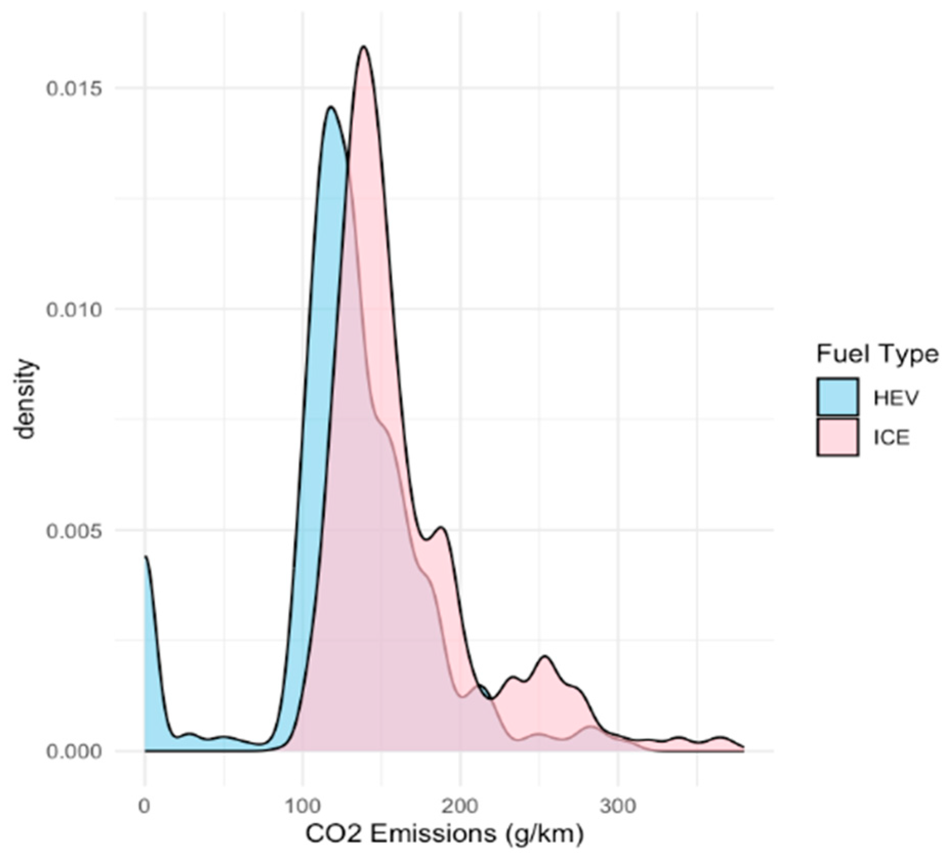
Complementing this, Figure 2 shows kernel density estimates of CO₂ emissions for ICE and HEV. The distribution for HEVs is shifted to the left, with a distinct concentration below 150 g/km, while ICE vehicles exhibit a broader and right-skewed distribution extending beyond 300 g/km. This contrast emphasizes not only lower central tendencies but also reduced variability among HEVs, reinforcing their relative environmental advantage.

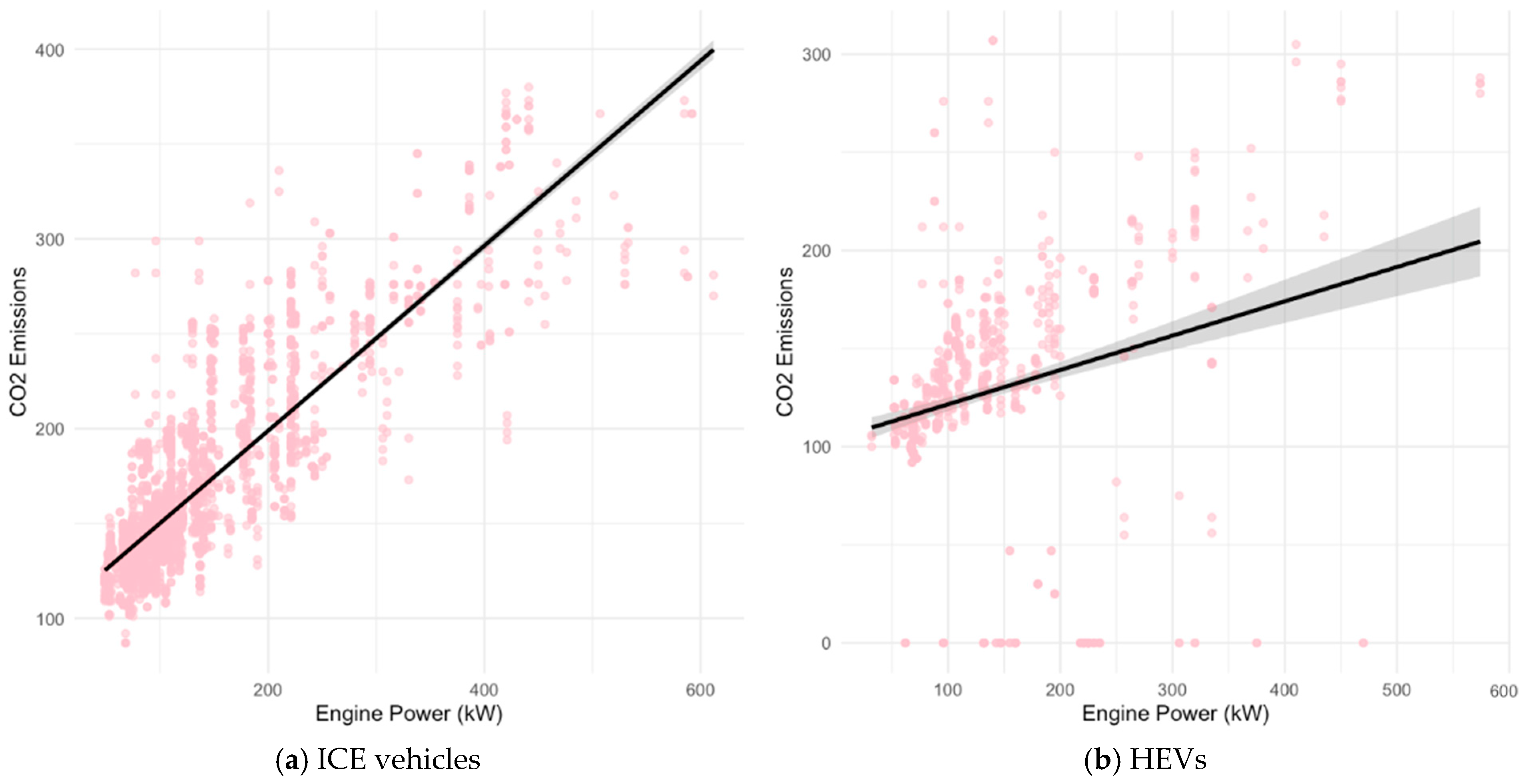
Figure 3 examines the bivariate relationship between engine power and CO₂ emissions. For ICE vehicles, emissions rise sharply with increasing power, particularly beyond 200 kW, illustrating the disproportionate environmental impact of high-performance engines. By contrast, HEVs also display a positive but less steep relationship, indicating that electrified powertrains partially decouple performance from emissions. Nevertheless, outliers at the high-power end highlight the limits of hybridization when vehicles rely more heavily on combustion engines under demanding conditions. These findings are consistent with engineering evidence that higher energy demand translates into elevated emissions despite efficiency gains [28].

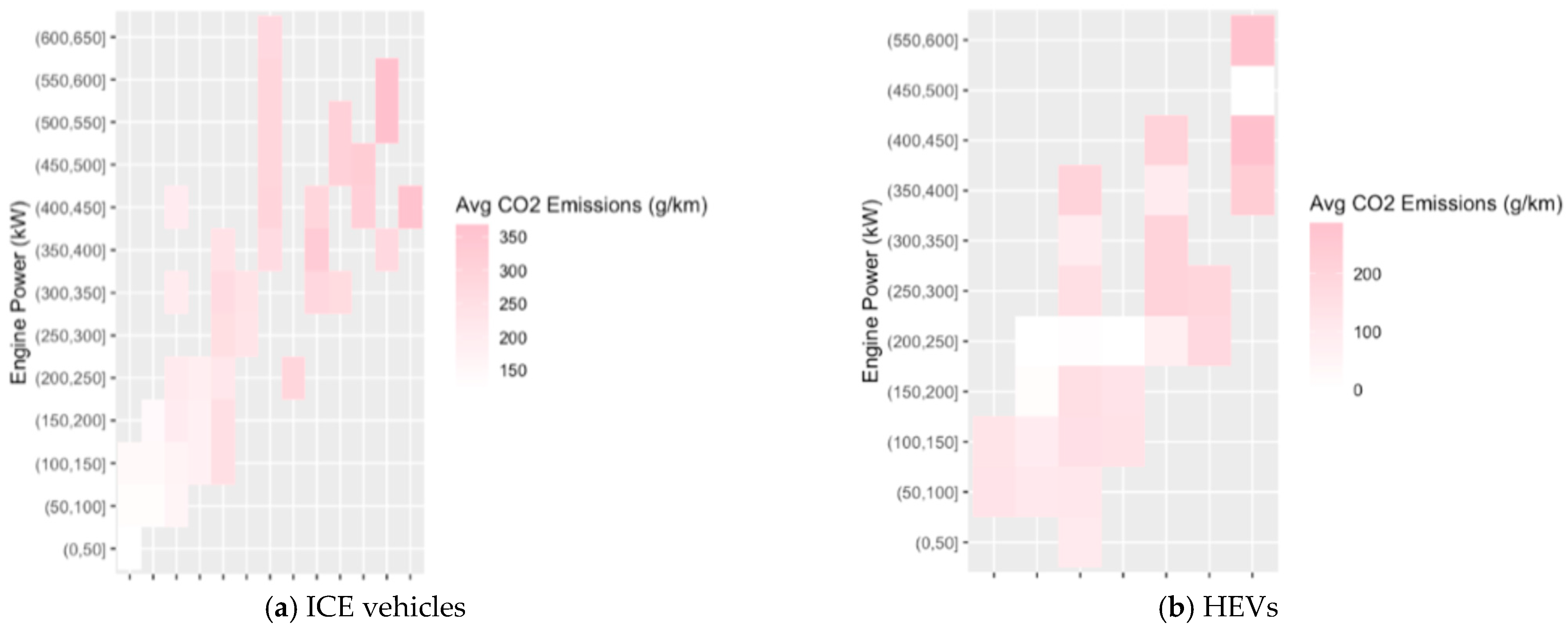
Finally, Figure 4 provides heatmaps of engine capacity, engine power and average CO₂ emissions, disaggregated by ICE and HEV, respectively. Both categories reveal clear patterns: vehicles with larger displacement and higher power output tend to occupy zones of higher average emissions. However, HEVs cluster more densely in lower emission ranges across similar capacity and power bands, indicating a technological advantage in reducing marginal emissions for given engine specifications. This pattern provides an important rationale for retaining both engine power and engine capacity as explanatory variables in subsequent models while also suggesting that HEVs mitigate (but do not eliminate) the structural link between technical specifications and environmental outcomes.

4.2. Model Performance

Table 3. Model performance comparison.

	ICE			HEV
	MSE	RMSE	R2	MSE	RMSE	R2
Linear Regression	0.00193	0.04396	0.739	0.01963	0.14012	0.739
Random Forest	0.00019	0.01373	0.996	0.01416	0.11898	0.812
Decision Tree	0.00217	0.04662	0.966	0.01491	0.12209	0.802
XGBoost	0.00019	0.01398	0.997	0.00076	0.02755	0.989

reports the predictive performance of the four machine learning models across both the ICE and HEV datasets. For ICE vehicles, ensemble methods achieved outstanding predictive accuracy. Both Random Forest and XGBoost recorded MSE below 0.0002 and RMSE values around 0.014, corresponding to explained variance (R²) exceeding 0.996. These results demonstrate the high stability of ICE emission patterns, where CO₂ output is tightly coupled with technical specifications such as fuel consumption and engine displacement. By contrast, linear regression explained only 74% of the variance ($R^2=0.739$), and its RMSE was three times higher, underscoring the inadequacy of purely linear models in capturing the complexity of vehicular emissions.

In HEVs, predictive accuracy was generally lower, reflecting the greater variability introduced by hybrid energy management and switching between combustion and electric modes. Nevertheless, XGBoost clearly outperformed all other models, achieving an RMSE of 0.0276 and an R² of 0.989. This represents a nearly 80% reduction in error compared to linear regression ($RMSE=0.140,R^2=0.739$) and a substantial gain over Random Forest ($RMSE=0.119,R^2=0.812$). These results confirm that gradient boosting is particularly effective in handling the nonlinearities and interaction effects inherent in hybrid vehicles. Importantly, while HEV emissions are more difficult to predict, XGBoost delivers robust performance across both vehicle types, providing a strong foundation for subsequent explainable analysis.

From an environmental perspective, these findings are significant. The high predictability of ICE emissions reflects their structural dependence on fuel use, whereas the greater variability in HEV emissions underscores the challenges of assessing emerging technologies with more complex operating regimes. By demonstrating that XGBoost consistently delivers superior predictive performance, this study identifies a robust modeling approach that can be directly applied to emission monitoring and policy analysis. It contributes to the evidence base needed to support SDG 13: Climate Action, which calls for urgent measures to mitigate climate change and its environmental impacts.

4.3. Feature Importance Comparison

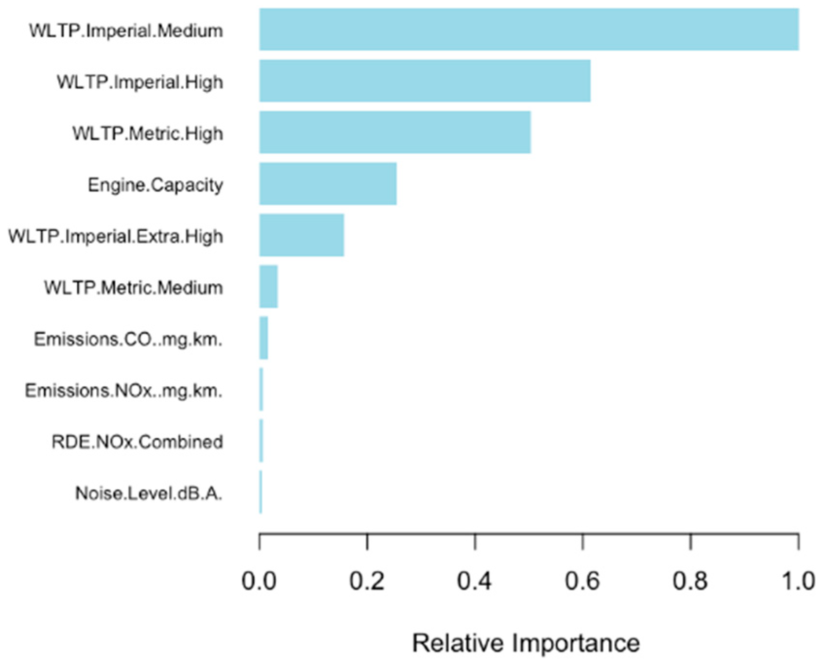
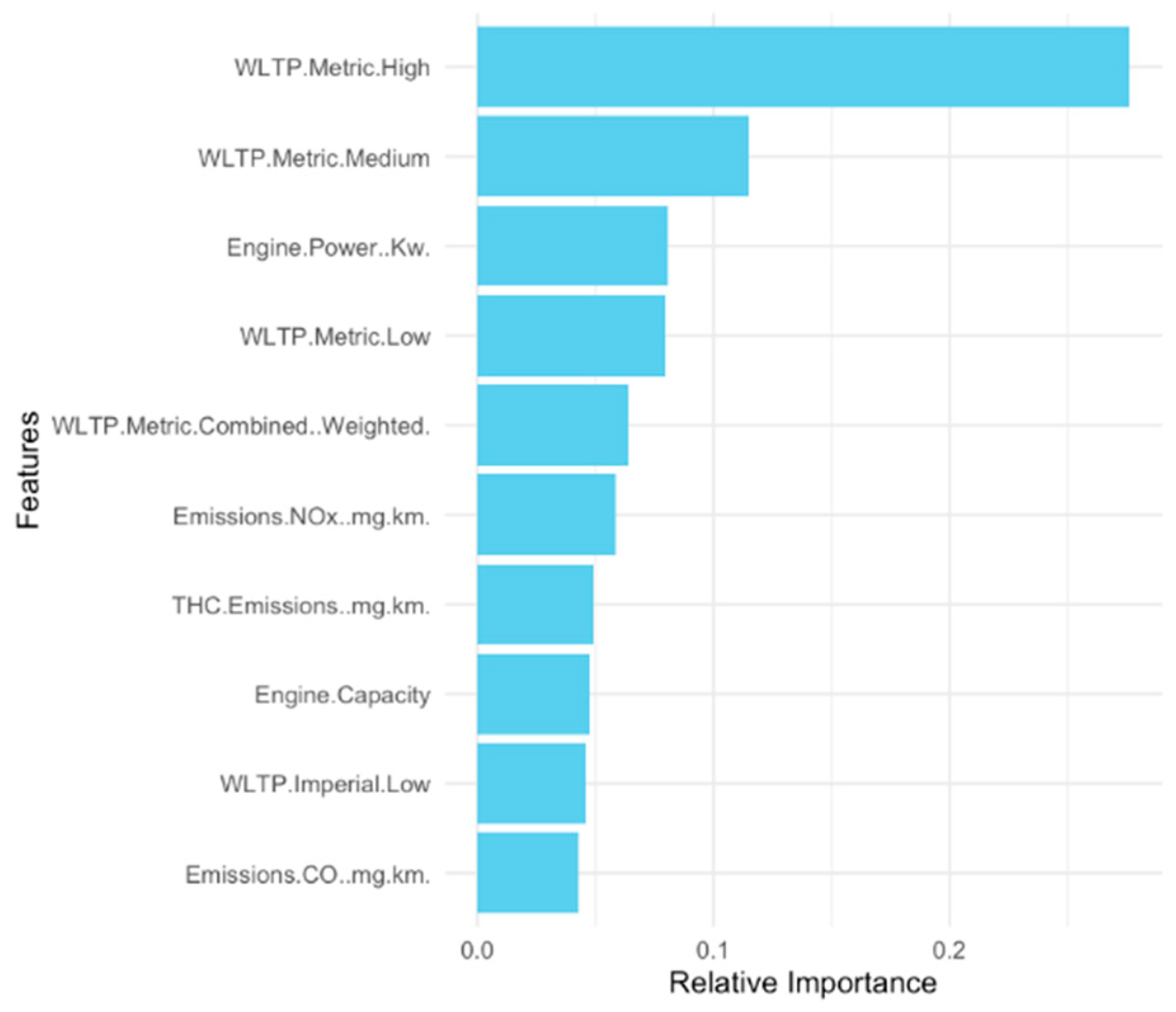
Figure 5 and Figure 6 compare the feature importance derived from the XGBoost models for ICE and HEVs. For ICE, the dominant predictors are fuel consumption under medium- and high-speed WLTP cycles, with “WLTP Imperial Medium” emerging as the most influential single variable. This reflects the strong structural dependence of CO₂ emissions on fuel economy during sustained driving regimes, where combustion efficiency is most decisive. Engine displacement also contributes substantially, reinforcing the well-established fuel-displacement-emission linkage [29]. By contrast, other attributes such as NO_X, CO and noise level show negligible influence in the ICE model, suggesting that, for conventional engines, emissions are overwhelmingly governed by core fuel-use characteristics rather than by secondary pollutant signals.

In HEVs, the importance profile is more diverse. “WLTP Metric High” is by far the most significant predictor, underscoring the persistent emission surges that occur when hybrids operate under high-load combustion conditions. Medium-speed fuel consumption and engine power also play meaningful roles, indicating that even with electrification, emission intensity remains partly tied to traditional performance variables. Notably, pollutant indicators such as NO_X and THC emissions show greater relative importance in the HEV model than in the ICE model. Their inclusion is not intended to suggest a mechanistic causal pathway from NO_X/THC to CO₂; rather, it reflects the fact that these pollutants are often co-produced with CO₂ under similar thermodynamic and combustion regimes. In this sense, their predictive value lies in capturing the co-pollutant dynamics of hybrid operation, where the switching between combustion and electric modes introduces greater variability in emission profiles.

The comparison highlights both commonalities and divergences across powertrains. In both ICE and HEV, speed-related fuel consumption measures dominate the predictive structure, identifying mid- and high-speed regimes as the most critical intervention points for emission mitigation. However, ICE emissions are structurally driven by displacement and efficiency in sustained combustion cycles, whereas HEV emissions are disproportionately sensitive to high-load operation and pollutant co-variation effects. This distinction carries clear environmental implications: for ICE fleets, downsizing and efficiency improvements in medium- to high-speed ranges remain the most effective levers for reducing emissions, while for HEVs, strategies should focus on optimizing hybrid control under high-load conditions and leveraging technologies that simultaneously reduce CO₂ and co-pollutants such as NO_X.

4.4. ICE: ALE Analysis

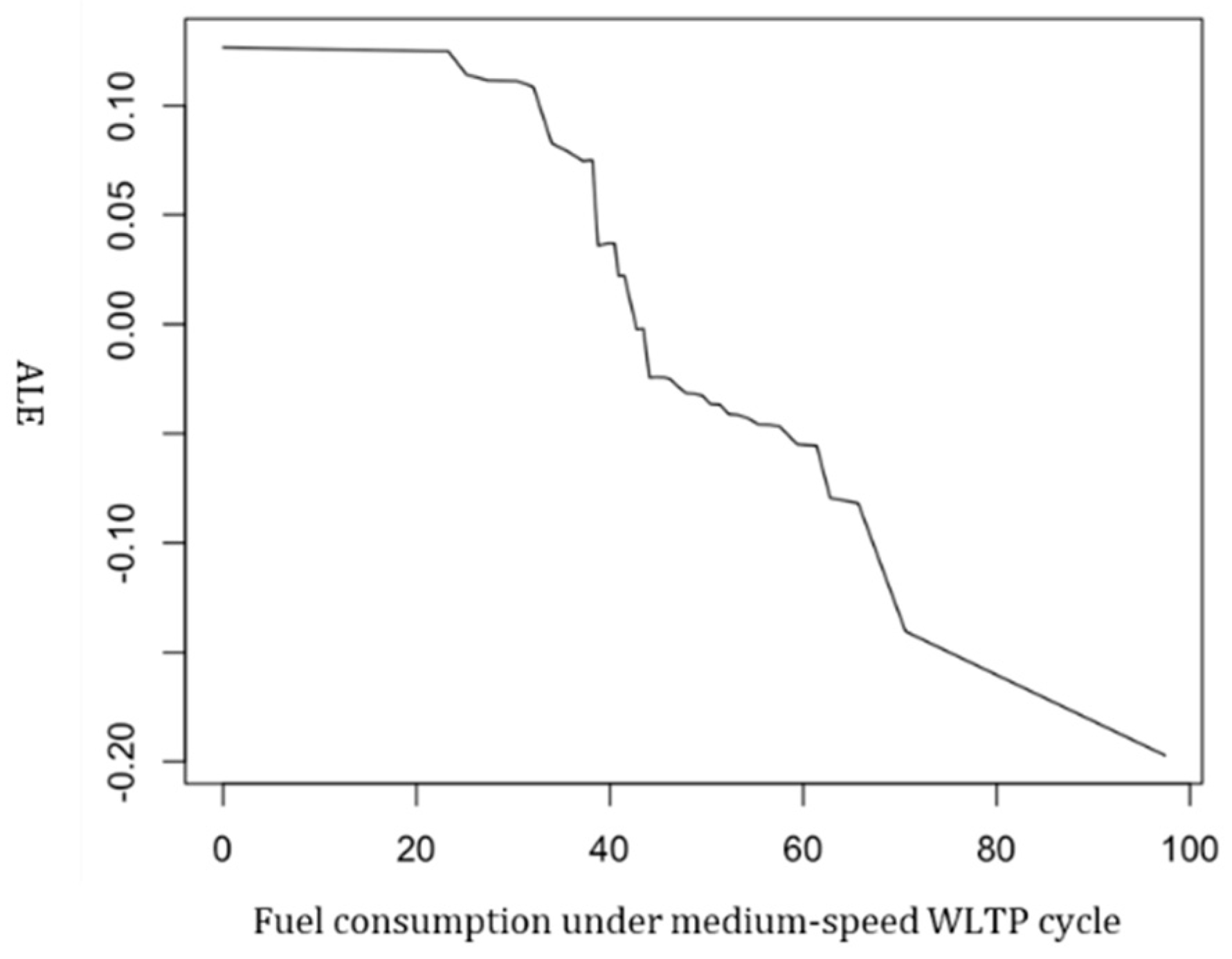
Figure 7 illustrates the ALE of WLTP Imperial Medium fuel consumption on CO₂ emissions from ICE vehicles. The curve shows a consistent negative slope, indicating that higher medium-speed fuel efficiency is strongly associated with reduced predicted emissions. The effect is relatively flat at very low values (0–10) and at the upper extreme (>50), but between 10 and 60 the decline is sharp, with the steepest reductions occurring in the 30–60 range. This pattern underscores the disproportionate impact of medium-speed operating conditions on emission intensity: improving efficiency in this regime yields substantial reductions in CO₂ output. Given that medium-speed driving corresponds to common inter-urban traffic conditions, these findings emphasize the importance of targeting efficiency gains in everyday driving cycles as a central lever for emission mitigation.

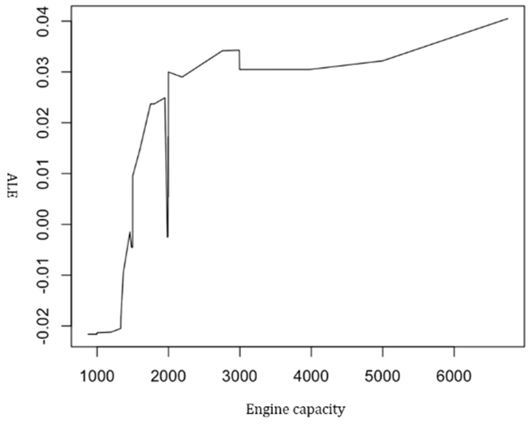
Figure 8 shows the ALE curve for engine capacity, which displays a clear positive association with CO₂ emissions. Emissions rise rapidly in the range of 1000–3000 cc, confirming that larger displacement engines consume more fuel and consequently produce higher CO₂ [29]. Beyond 3000 cc, the curve flattens, suggesting diminishing marginal effects at very high displacements. This plateau may reflect the adoption of advanced fuel technologies or partial efficiency gains in larger engines, although the overall emission burden remains higher than in smaller engines. A slight dip between 1500 and 2000 cc could point to segment-specific technologies, such as optimized combustion strategies or partial hybridization, that temporarily reduce emissions. Nonetheless, the dominant trend is upward, reinforcing the case for downsizing and for incentivizing low-displacement engines as an effective pathway for energy saving and carbon reduction.

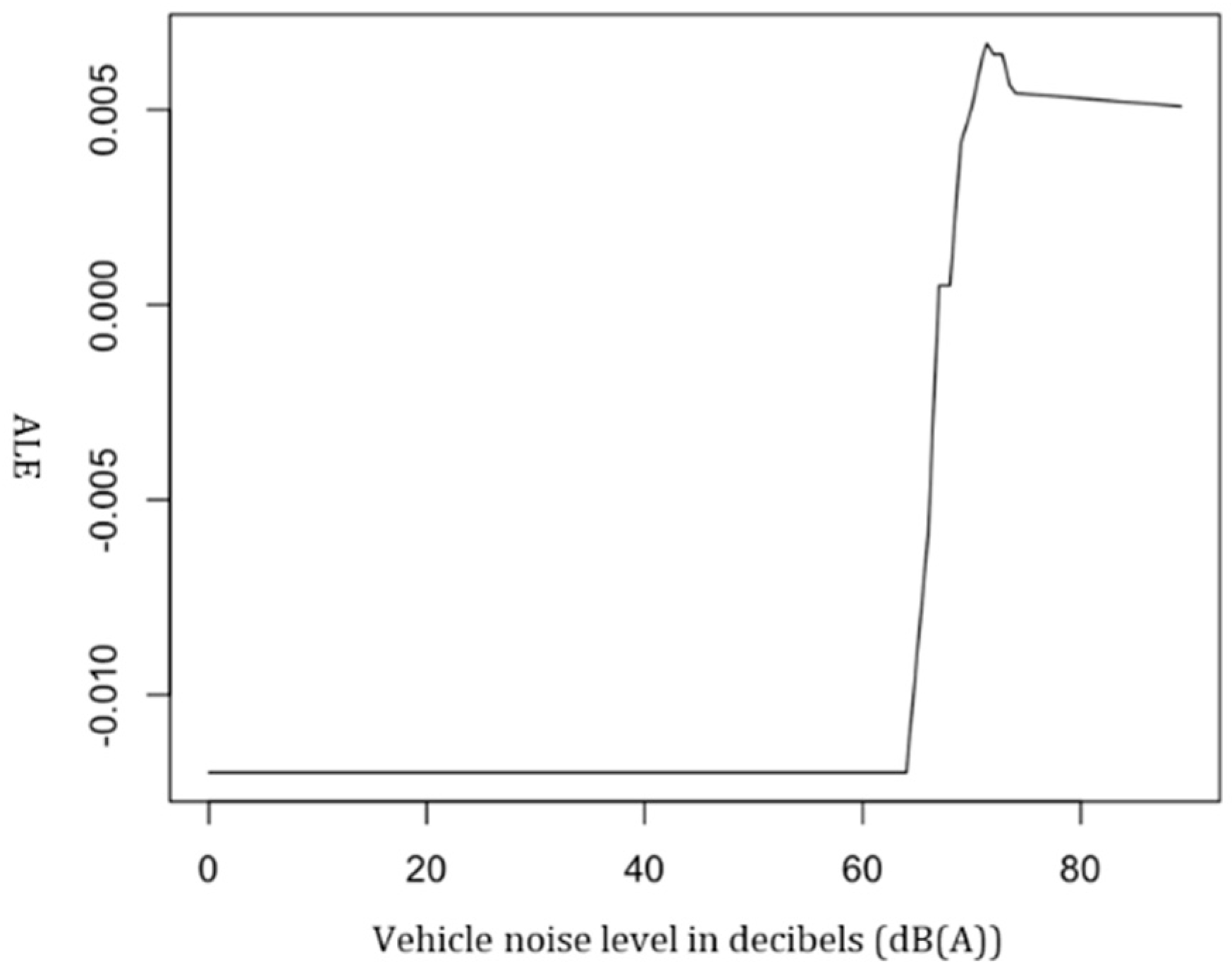
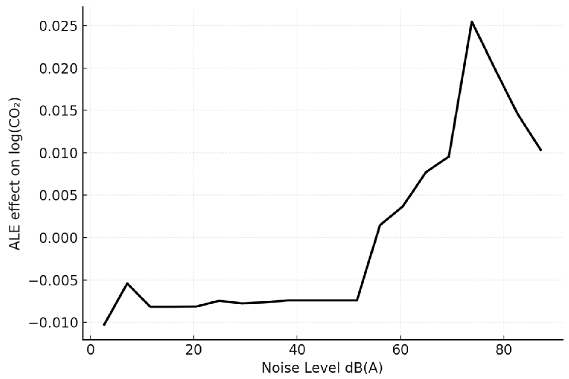
Figure 9 presents the ALE curve for Noise Level dB(A), introduced as an exploratory covariate to capture co-variation between acoustic and emission dynamics. The curve remains nearly flat at low noise levels, indicating no substantial association with CO₂ emissions under light-load or low-speed conditions. However, once noise exceeds approximately 60 dB(A), the curve rises sharply, suggesting that higher acoustic levels coincide with combustion regimes characterized by greater fuel consumption and higher CO₂ output. The effect stabilizes beyond 80 dB(A), indicating a threshold beyond which additional increases in noise contribute little further to emissions. This threshold effect is consistent with the interpretation that noise acts as a proxy for high-load operation or aggressive driving. From an environmental perspective, the result highlights a potential co-benefit: strategies that reduce vehicle noise, such as speed management or design improvements, may also indirectly lower CO₂ emissions, aligning with integrated pollution control objectives [16].

4.5. HEVs: ALE Analysis

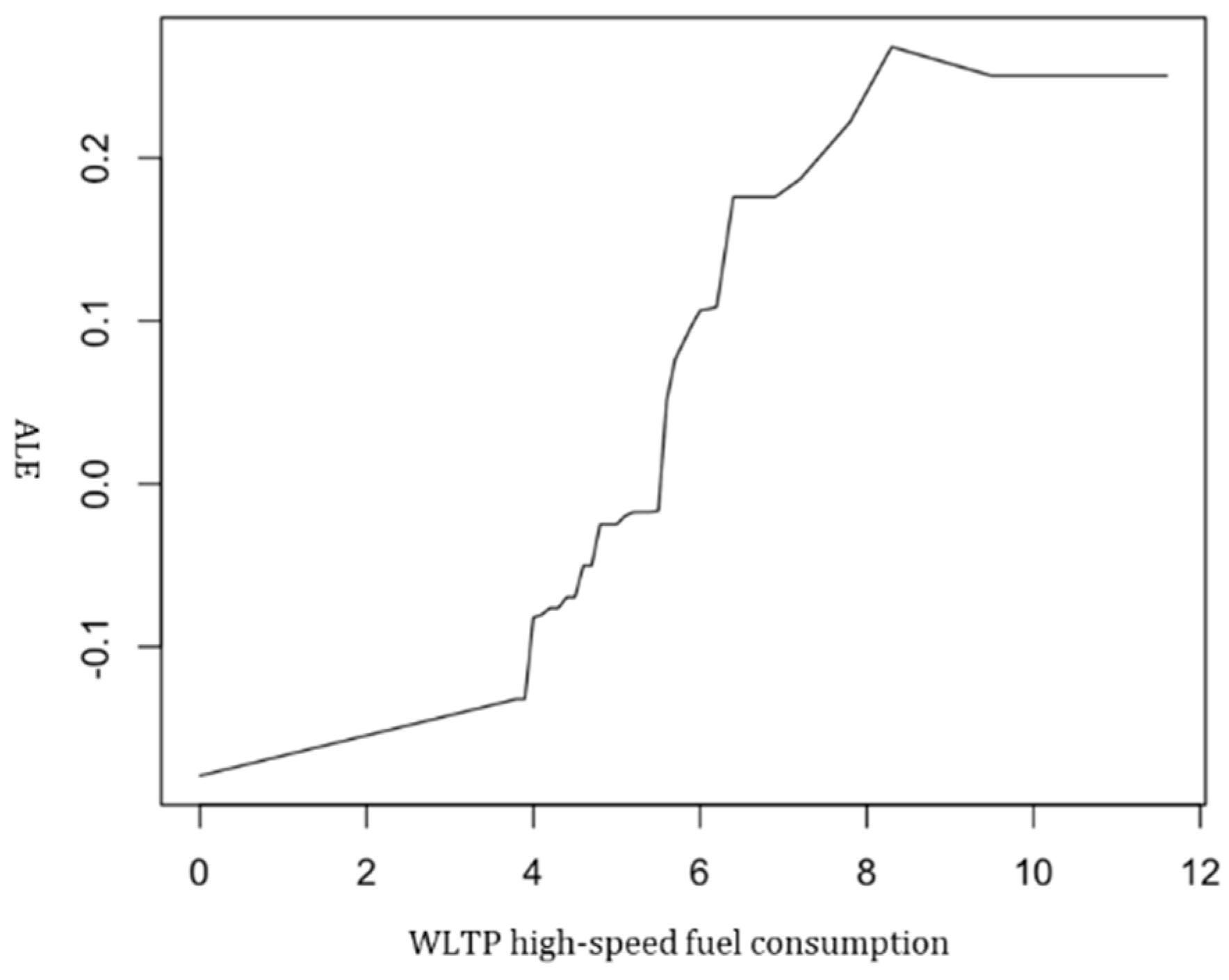
Figure 10 presents the ALE curve for WLTP Metric High fuel consumption in HEVs. The curve reveals a strong positive association with CO₂ emissions once values exceed approximately 4 L/100 km. In the low-load regime (<4), the effect is negligible or even slightly negative, consistent with the ability of HEVs to operate efficiently or partially in electric mode under light driving conditions [30]. However, between 4–6 the curve rises steeply, showing that fuel consumption at high loads is a decisive driver of CO₂ output. Beyond 6, the marginal effect flattens, suggesting that, after a certain threshold, additional increases in fuel consumption contribute proportionally less to emission growth. This finding highlights the critical importance of reducing fuel use in mid-to-high load scenarios, where hybrid powertrains rely more heavily on combustion engines, and the electric contribution is diminished.

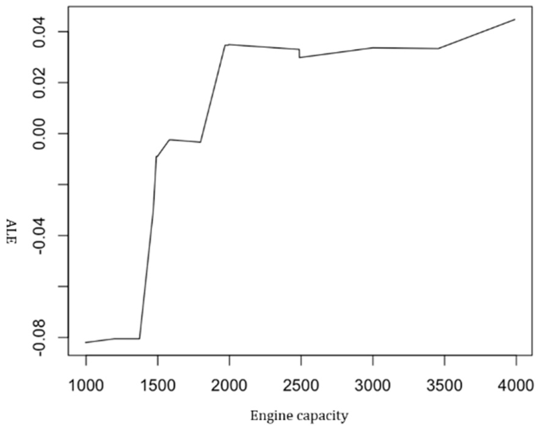
Figure 11 shows the ALE curve for engine capacity. As expected, larger displacements are associated with higher CO₂ emissions, with the steepest rise occurring between 1500–2000 cc. This reflects the transition point where engines shift from compact, relatively efficient configurations into higher-output designs that require significantly greater fuel input [22]. Beyond 2000 cc, emissions continue to increase but at a reduced marginal rate, possibly due to the adoption of advanced fuel management systems or partial hybrid assistance. Notably, the near-flat region below 1500 cc indicates that compact HEVs achieve substantial emission savings, reinforcing the environmental benefit of smaller displacement designs. For policy, this suggests that incentivizing medium-displacement efficiency and encouraging hybrid downsizing can yield tangible carbon reduction benefits.

Figure 12 illustrates the effect of NO_X emissions on CO₂ predictions. At very low NO_X levels (<10 mg/km), the ALE curve is negative or close to zero, reflecting stable combustion conditions with limited impact on CO₂. However, once NO_X exceeds 10 mg/km, the curve rises sharply, peaking around 30–40 mg/km. This positive correlation highlights the co-pollutant dynamics of combustion: higher NO_X formation generally corresponds to elevated combustion temperatures and fuel throughput, which simultaneously increase CO₂ emissions. At extreme NO_X levels, the marginal effect diminishes, suggesting a saturation point where both pollutants stabilize. From an environmental perspective, this co-variation reinforces the importance of integrated aftertreatment technologies such as Selective Catalytic Reduction (SCR) and Exhaust Gas Recirculation (EGR), which can simultaneously mitigate NO_X and CO₂, thereby addressing multiple regulatory targets under stricter emission standards.

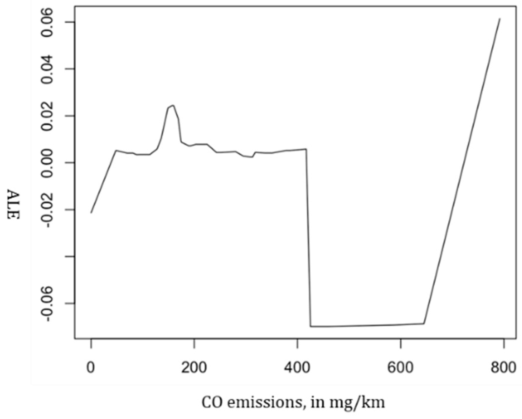
Figure 13 depicts the ALE curve for CO emissions, which exhibits a more complex pattern. At low to moderate ranges (0–400 mg/km), the effect on CO₂ is minimal, with ALE values fluctuating close to zero. This suggests that moderate CO emissions do not systematically drive CO₂ variation, likely reflecting differing combustion pathways. However, beyond 400 mg/km the curve first drops sharply, then rebounds strongly after 600 mg/km, where CO₂ emissions increase markedly. This nonlinear relationship indicates that, under certain extreme combustion conditions, inefficient fuel oxidation may temporarily decouple CO from CO₂ output, but, once thresholds are exceeded, both pollutants rise dramatically. These dynamics highlight the role of combustion efficiency and exhaust gas aftertreatment in shaping multi-pollutant outcomes, with implications for both carbon and air quality regulation.

Figure 14 presents the ALE curve for Noise Level dB(A) in HEVs, introduced as an exploratory covariate to capture the interaction between acoustic conditions and CO₂ emissions. The curve remains essentially flat at lower noise levels (below 55 dB(A)), indicating that when vehicles operate in low-load conditions or in electric-drive mode, acoustic intensity has negligible association with carbon output. Beyond approximately 60 dB(A), the curve begins to rise gradually, reflecting the transition toward combustion-dominant operation, where increases in engine load and fuel consumption manifest as both higher noise and greater CO₂ emissions. The effect plateaus above 80 dB(A), suggesting a saturation threshold in which additional acoustic increments contribute little further to emission levels.

4.6. Comparative Insights Between ICE and HEV

The comparative ALE and feature importance analyses highlight fundamental differences in the determinants of CO₂ emissions between ICE vehicles and HEVs. For ICEs, emissions are strongly shaped by fuel consumption under medium- and high-speed cycles, reflecting their structural dependence on direct combustion efficiency. Engine displacement further reinforces this trend, with larger engines yielding disproportionately higher emissions until technical plateaus are reached. These results emphasize the inherent constraints of conventional combustion technologies: even with incremental efficiency improvements, high-speed operation and larger displacements consistently exacerbate carbon output.

By contrast, HEVs display a more nuanced emissions profile. While engine capacity remains influential, the dominant drivers are fuel consumption under high-load conditions and pollutant co-variation with NO_X. This suggests that hybridization moderates emissions in low-load conditions (often by leveraging electric drive) but loses this advantage under sustained high loads when combustion predominates. Moreover, the positive association between NO_X and CO₂ in HEVs reveals an important co-pollutant dynamic: hybrid vehicles, though marketed as environmentally friendly, can still generate significant emissions when operating in modes that favor combustion power.

In both vehicle types, the inclusion of noise level as an explanatory variable provides an additional environmental dimension. The ALE results showed that higher noise levels, typically above 60 dB(A), are associated with increased CO₂ emissions, reflecting the fact that acoustic intensity is a proxy for aggressive driving conditions, high speeds or elevated engine loads. This finding indicates that noise pollution is not only a social and health externality but also a co-indicator of carbon intensity in road transport. As such, integrated policies targeting urban noise abatement, such as stricter vehicle acoustic standards, road surface improvements and traffic calming measures may deliver dual benefits for both environmental health and climate mitigation.

From a policy perspective, these differentiated findings point to tailored interventions. For ICE vehicles, policies that constrain engine size and impose stricter efficiency standards at medium-to-high speeds are most likely to yield significant reductions. For HEVs, strategies should prioritize extending electric operating ranges, improving combustion efficiency at high load, and deploying advanced aftertreatment systems such as SCR and EGR to simultaneously mitigate NO_X and CO₂. Crucially, the observed role of noise underscores the value of multisectoral policy design that connects vehicle technology standards with urban planning and environmental quality objectives.

Policy implications extend beyond vehicle design. The dominance of speed- and load-related variables in both ICE and HEV models highlights the systemic drivers of transport emissions. Infrastructure and behavioral measures such as speed enforcement, differentiated road pricing and urban design favoring lower-speed mobility can reduce both CO₂ and noise, offering co-benefits for climate, air quality and public health. These measures dovetail with SDG 13 (Climate Action), which calls for urgent mitigation of anthropogenic climate drivers while safeguarding broader environmental well-being.

In sum, while HEVs offer advantages over ICEs in low-load conditions, their environmental benefits are conditional rather than absolute. A robust climate policy must therefore treat hybridization not as an endpoint but as a transitional measure toward full electrification, complemented by demand-side policies that reshape mobility patterns and address coupled environmental stressors, including noise and emissions under high-load regimes. These integrated approaches will be critical for aligning vehicle technology development with global climate and sustainability objectives.

5. Conclusions

This study analyzed CO₂ emissions from ICE and HEVs using a suite of machine learning models, complemented by explainable AI techniques. XGBoost provided the most accurate and robust predictions, but, more importantly, its integration with ALE enabled the disentangling of nonlinearities and interaction effects, offering a transparent understanding of how technical and contextual factors jointly shape vehicle emissions.

The findings highlight differentiated and conditional emission mechanisms across vehicle types. For ICEs, emissions are predominantly driven by engine displacement and speed-related fuel consumption, highlighting the structural dependence of conventional combustion engines on load and efficiency. For HEVs, emissions remain stable under low- to medium-load operation, reflecting the moderating role of electrification, but increase sharply under sustained high-load driving, when combustion predominates. This conditional advantage of HEVs emphasizes that their environmental benefits are situational rather than absolute. Additionally, the persistence of a strong positive association between NO_X and CO₂ in HEVs reveals a co-pollutant dynamic that is less frequently highlighted in prior literature.

A further methodological innovation is the integration of noise level as an explanatory variable. ALE analysis revealed a threshold-type effect: emissions remain stable below 55–60 dB(A), but rise steadily at higher acoustic levels before stabilizing again, reflecting the coupling between acoustic intensity, driving aggressiveness and combustion demand. This finding suggests that noise pollution, typically treated as a social or health issue, can also act as an environmental proxy for carbon intensity, offering a novel cross-cutting indicator that connects traffic emissions with urban acoustic management.

From a policy perspective, these insights point to differentiated and multisectoral strategies. For ICEs, downsizing, aerodynamic optimization and stricter efficiency standards under medium-to-high loads remain central levers for mitigation. For HEVs, the priority lies in extending electric operating ranges, improving combustion efficiency at high loads, and integrating advanced aftertreatment systems such as SCR and EGR to mitigate coupled CO₂-NO_X emissions. More broadly, the recognition of speed- and load-related factors, together with the role of noise, underscores the need for system-level measures, such as speed enforcement, congestion pricing, and noise abatement, that can simultaneously deliver climate, air-quality, and public-health benefits.

In conclusion, this study contributes novelty in three ways: (1) moving beyond expected mean differences between ICEs and HEVs by uncovering conditional, mechanism-oriented patterns of emissions, including the erosion of HEV advantages under high load and the persistence of CO₂-NO_X co-dynamics; (2) introducing noise as a seldom-used but informative contextual proxy, identifying a threshold-type relationship that links acoustic and carbon outcomes; and (3) demonstrating the value of explainable machine learning for environmental applications, producing insights that are both scientifically transparent and policy-relevant. These contributions advance methodological practice, enrich empirical understanding, and provide a stronger evidence base for integrated strategies in sustainable transport and climate action.

A limitation of this study is the absence of explicit variables on engine boosting or manifold pressure, which are important for modern turbocharged engines. Although engine power and fuel consumption partially capture their influence, future research would benefit from datasets including direct boosting parameters.