Abstract
Establishing accurate models for central air-conditioning systems is an indispensable part of energy-saving optimization research. This paper focuses on large commercial buildings and conducts research on improving the energy efficiency model of chillers in central air-conditioning systems based on meta-learning. Taking the Model-Agnostic Meta-Learning (MAML) framework as the core, the study systematically addresses the energy efficiency prediction problem of chillers under different operating conditions and across different equipment. It constructs a comprehensive research process including data preparation, meta-model training, fine-tuning and evaluation, cross-device transfer, and energy efficiency analysis. Through its bi-level optimization mechanism, MAML significantly enhances the model’s rapid adaptability to new tasks. Experimental validation demonstrates that: under varying operating conditions on the same device, only 5 data points are required to achieve a relative error (RE) within 3%; under similar operating conditions across different devices, 4 data points achieve a RE within 5%. This represents a reduction in data requirements by 50% and 73%, respectively, compared to standard Multi-Layer Perceptron (MLP) models. This method effectively addresses modeling challenges in complex operating scenarios and offers an efficient solution for intelligent management. It significantly enhances the model’s rapid adaptation capability to new tasks, particularly its generalization performance in data-scarce scenarios.
1. Introduction
With the acceleration of global urbanization and the improvement of living standards, building energy consumption has become increasingly significant in the total energy consumption, reaching 30% of the nation’s total energy use. Central air-conditioning systems, as the primary energy consumers in commercial buildings, account for approximately 40–60% of the total building energy consumption [1,2]. Against the backdrop of tightening energy resources and intensifying climate change, the efficient operation and energy-saving optimization of central air-conditioning systems have emerged as critical issues for achieving green buildings and sustainable development. However, several challenges persist in the current operation of central air-conditioning systems. Firstly, traditional operating strategies predominantly rely on fixed-parameter control, lacking adaptability to dynamic loads and environmental changes [3,4], which results in energy redundancy and wastage. Secondly, key components such as chillers, water pumps, and cooling towers operate independently despite their strong coupling, leading to insufficient coordination and suboptimal overall system energy efficiency [5]. Additionally, performance curves of core equipment (e.g., chillers, pumps, cooling towers) drift over time due to aging, resulting in inadequate modeling accuracy, poor model adaptability, and limited real-time optimization capabilities. These limitations further constrain the exploration of energy-saving potential, particularly in data-scarce scenarios or under complex operating conditions. Collectively, these issues contribute to low operational efficiency and persistently high energy consumption.
Establishing accurate models of central air-conditioning systems is an indispensable component of energy-saving optimization research. After predicting cooling loads, inputting load data and environmental parameters into the chiller plant model enables simulation of the system’s overall energy consumption under different control strategies, thereby guiding the operation of field equipment [6,7]. Currently, white-box models [8] are widely adopted in mainstream building simulation software such as TRNSYS 18, EnergyPlus 25.1.0, Dymola 2025, and DeST 2.0. However, most white-box models are highly complex; as the scale of central air-conditioning systems increases, computational difficulty rises sharply, making them impractical for real-time control scenarios. Commonly used black-box modeling approaches in this domain include artificial neural networks (ANNs) [9,10,11], support vector regression (SVR) [12,13], and random forests (RF) [14,15]. Compared with white-box methods, black-box modeling offers lower implementation complexity and broader applicability, eliminating the need for intricate derivations. Nevertheless, the accuracy of black-box models heavily depends on the quality and quantity of training datasets, with predictive performance significantly degrading under operating conditions outside the training scope. Grey-box modeling [16,17,18]—a hybrid approach integrating white- and black-box methods—derives its fundamental structure from physical principles while determining internal parameters through identification using actual operational data. Combining the strengths of both paradigms, grey-box modeling has gained substantial traction in recent applications.
To address these limitations, this paper proposes an improved strategy to reduce the training data requirements of equipment models while enhancing their generalization capabilities. Specifically for chiller modeling, we adopt a neural network framework enhanced by meta-learning. This approach not only significantly decreases the volume of training data needed during equipment modeling but also improves the model’s adaptability to unseen operating conditions. Consequently, it provides enhanced model feasibility assurance for optimizing central air-conditioning systems.
2. Model Establishment and Solution
2.1. Methodological Overview
Meta-learning [19], also referred to as “learning to learn”, focuses on designing algorithms that understand and optimize the learning process itself. It trains models to capture common characteristics across different tasks, thereby obtaining generalized parameters applicable to all tasks, which enables rapid adaptation to new tasks.
In meta-learning, tasks are divided in a more refined manner, including training tasks and test tasks. The dataset of a training task is further split into a support set and a query set. The support set provides the model with a set of specific task examples for training and fine-tuning. By learning from the support set, the model acquires the basic features and patterns of the task, forming a preliminary understanding. The query set is used to evaluate the prediction accuracy of meta-learning on a specific task. After the model learns task-related knowledge from the support set, the query set provides a different set of data samples to validate the model’s learning effectiveness and generalization capability.
This study employs Model-Agnostic Meta-Learning (MAML) [20], a classical method in meta-learning. MAML adjusts the initial parameters of the model so that it can quickly converge to a state adapted to a new task with only a few samples. Reptile [21] is another common meta-learning algorithm. It performs multiple iterations on each task, enabling the model parameters to align with the directions of multiple tasks, thus facilitating rapid adaptation to few-shot learning scenarios. Table 1 summarizes the key differences and comparative advantages between MAML and Reptile.

Table 1.
Comparison between MAML and Reptile.
In this study, meta-learning is primarily applied to investigate the transfer learning of chiller energy efficiency models. Chiller operating conditions (e.g., load, temperature, humidity) vary significantly, and physical characteristics differ across different units. MAML demonstrates stronger performance in cross-domain transfer and few-shot learning, making it more suitable for meeting the requirements of optimized control and performance prediction.
2.2. Model Selection and Establishment
2.2.1. Baseline Model Selection
Accurate equipment energy consumption modeling is crucial for achieving optimal energy-saving effects in the centralized control of central air-conditioning systems. Existing modeling approaches for air-conditioning system equipment primarily include white-box (mechanism-based) modeling, polynomial regression modeling, and neural network modeling. As white-box modeling is unsuitable for studying equipment dynamic characteristics, this study focuses on comparing polynomial and neural network models. Based on historical data obtained from the energy management platform, the performance and generalization capability of these two models are compared, with the superior model selected as the foundation for subsequent optimization research.
Previous studies indicate that chiller energy consumption is related to condensing temperature, evaporating temperature, and unit load [22]. Specifically, during chiller operation, the condensing temperature is primarily determined by the cooling water supply temperature (Tcw,s), while the evaporating temperature is closely associated with the chilled water supply temperature (Tchw,s). Accordingly, an energy consumption model is proposed based on chilled water supply temperature, cooling water supply temperature, and unit load. The polynomial model employs a complete quadratic regression approach to establish a mathematical relationship between chiller energy consumption and these three operating parameters. Complete quadratic regression models are widely used in statistics to investigate complex relationships among variables. By incorporating squared terms and interaction terms, this model effectively captures nonlinear relationships and interactions between variables.
For the neural network-based chiller energy efficiency model, the input and output parameters remain consistent with the polynomial model: Tcw,s, Tchw,s, and part load ratio (PLR). The multilayer perceptron (MLP) neural network is commonly used for establishing chiller energy efficiency models. As a classic feedforward artificial neural network, MLP consists of at least three layers of nodes: an input layer, one or more hidden layers, and an output layer. It can be trained using the backpropagation algorithm to adjust weights and minimize errors. Through its hidden layers, the MLP neural network can learn complex nonlinear relationships in chiller operational data and accurately predict chiller energy efficiency parameters, thereby providing a reliable model for chiller optimization control.
To compare the advantages and disadvantages of the polynomial and neural network models, the root mean square error (RMSE) is evaluated using different splits of the dataset into training and testing sets. As shown in Figure 1, under different data split ratios, the MLP model consistently demonstrated lower errors on both training and testing sets compared to the polynomial model. Therefore, the MLP neural network is selected in this study to characterize chiller performance.
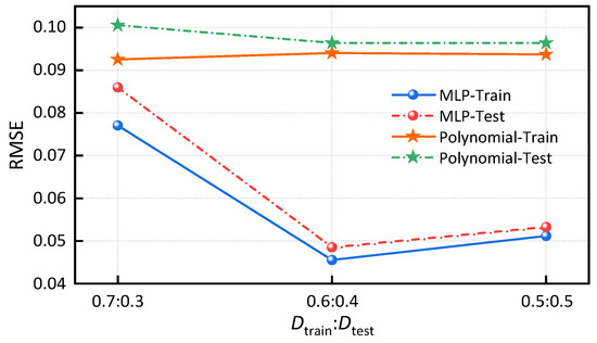
Figure 1.
Comparison of RMSE between the two models under different data split ratios.
This study employs a standard MLP as the primary baseline model to ensure clear and fair comparisons. This selection aims to isolate the performance improvement attributable to the meta-learning framework rather than to more complex network architectures. The MLP serves as a robust representative of mainstream data-driven modeling approaches in this field, effectively capturing the characteristics of conventional modeling methods.
2.2.2. Model Establishment and Solution Algorithm
The establishment process of the MAML model for the chiller is illustrated in Figure 2. Based on the chiller energy efficiency model, MLP neural network architecture is employed. The model takes three input features: Tcw,s, Tchw,s, and PLR. The output variable is the coefficient of performance (COP). The network architecture features a single hidden layer (using the ReLU activation function) and an output layer to model the input data. The objective of the model is to obtain, through training, a set of generalizable parameters. These parameters enable the model to adapt to new tasks with only a few gradient updates. Therefore, the models must satisfy the following assumptions and conditions: (1) The chiller’s COP is primarily governed by the three chosen input features under steady-state or quasi-steady-state operation. Transient dynamics are not considered; (2) The operational data used for training and testing are assumed to be representative of the chiller’s normal operating envelope; (3) The tasks (different setpoints or different chillers) are assumed to share underlying common knowledge that can be meta-learned, enabling transfer.
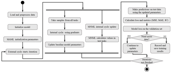
Figure 2.
MAML modeling process.
The inner loop is the core component of the MAML model, designed to enable the model to quickly adapt to the specific data of each task. For each task, the model starts from its initial parameters and fine-tunes them through the inner loop updates to improve its performance on that task. The inner loop typically includes the following steps: Calculate loss: The model performs forward propagation on the training set of the current task and calculates the prediction loss. For regression problems, we use mean squared error (MSE) as the loss function. Calculate gradients: Computes the gradients of the loss function with respect to the model parameters via backpropagation. Update parameters: Updates the model parameters using gradient descent based on the computed gradients.
The outer loop is used to update the initialization parameters of the model, enabling the model to quickly adapt to multiple tasks. In each round of the outer loop: the inner loop performs inner-loop fine-tuning on each task to generate task-specific parameters; the outer loop updates the loss calculated based on the test sets of multiple tasks and performs gradient updates.
Regarding optimizer configuration, In the inner loop, explicit gradient descent updates are employed. This means the computed gradients are used directly for simple gradient descent parameter updates. This approach is chosen to maintain computational efficiency and enable rapid adaptation within the inner loop, as only a few update steps are performed per task. In the outer loop, the Adam with Weight Decay (AdamW) optimizer is used. This sophisticated optimizer provides an advanced method for optimizing the model’s initial parameters. AdamW, leveraging both adaptive learning rates and momentum, is capable of more effectively optimizing the global parameters across multiple tasks.
Figure 3 shows the framework for training the MAML-based energy efficiency model for chillers. First, operational data is collected from air conditioning equipment using sensors and other devices. Then, the operational data is divided into datasets and preprocessed to construct a dataset for the meta-learning process. Next, meta-learning training and testing are performed using the training set and test set in the training task.
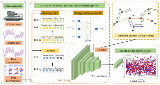
Figure 3.
Model architecture diagram of energy efficiency model transfer learning based on MAML.
The specific algorithm solution process is as follows: (1) First, initialize the parameters, the outer loop learning rate α, the inner loop learning rate β, the number of outer loop iterations ITEROuter, and the number of inner loop iterations ITERInner; (2) Divide the chiller unit operation dataset into training tasks (ΦA) and testing tasks (ΦB) according to the training objective, and further divide the training and testing tasks into training sets (Dtrain) and testing sets (Dtest) respectively. Thus, we have ΦA = {(, ), (, ), …, (, )}, ΦB = {(, ), (, ), …, (, )}; (3) Initialize the parameters of the meta-learner; (4) Select a set of data from the training set Dtrain on ΦA for the inner loop gradient update, with the update count being the number of inner loop iterations. Pass the updated inner loop parameters to the outer loop; (5) Select a set of data from the test set Dtest on ΦA for the outer loop gradient (meta-gradient) update, with the update count equal to the number of iterations in the outer loop. Save the updated outer loop parameters (meta-parameters); (6) Select a set of data from the training set Dtrain on ΦB for gradient update, i.e., parameter fine-tuning, so that the model with the previously trained meta-parameters can quickly adapt to the target task. Evaluate the performance of the fine-tuned model on the target task and save the optimal model after training.
2.3. Dataset and Evaluation Metrics
2.3.1. Dataset Introduction
All data for the chiller units required for this study were obtained from the energy management cloud platform of a shopping mall in Chengdu. The hourly operational data of two chiller units—Chiller Unit 1 (centrifugal type, model YKN3L7K25DCH, York, China, with a rated cooling capacity of 4920.3 kW) and Chiller Unit 2 (centrifugal type, model YKK6K4K15DAG, York, China, with a rated cooling capacity of 4216.9 kW)—were selected for analysis. The primary data collected include cooling water supply temperature Tcw,s, chilled water supply temperature Tchw,s, load factor PLR, and energy efficiency ratio COP. The dataset shows that the chilled water supply temperature Tcw,s ranges from 5 to 8 °C, the cooling water supply temperature Tcw,s ranges from 19 to 34 °C, the load factor PLR ranges from 20% to 100%, and the energy efficiency ratio COP ranges from 3.55 to 7.13.
The subject of this study is commercial buildings, with air conditioning operating from 10:00 to 22:00 daily. Taking typical summer working day data as an example, the operating data for centrifugal Chiller Unit 1 is summarized in Table 2.
Table 2.
Partial operating data for Chiller Unit 1.
2.3.2. Data Preprocessing and Standardization Strategy
The data processing pipeline established in this study comprises two core stages: data cleaning with feature reduction, and model input preprocessing. This integrated approach employs clustering-based sampling to eliminate redundant operating condition points, validates feature space effectiveness through principal component analysis (PCA) visualization, and ensures data quality via missing value inspection and a dual standardization scheme that separately handles feature and target scaling. The methodology forms a comprehensive end-to-end processing pipeline, with the specific architecture illustrated in Figure 4.
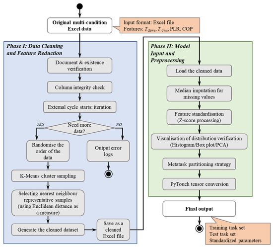
Figure 4.
Core architecture for data preprocessing.
In this study, to evaluate the model’s generalization capability across different scenarios, we designed two experimental approaches: one being different operating conditions on the same device, the other being cross-device scenarios (same equipment type) operating conditions. For different operating conditions on the same device, data from Chiller Unit 1 was split by Tchw,s. The subsets with Tchw,s = 5 °C, 6 °C, and 7 °C were used as ΦA, while the subset with Tchw,s = 8 °C was used as ΦB. This split is based on operating mode to simulate real-world scenarios where the model must adapt to previously unseen setpoints. For cross-device scenarios (same equipment type) operating conditions, data from Chiller Unit 1 was used as ΦA, and data from Chiller Unit 2 was used as ΦB. This evaluates transferability between devices of the same type but with different rated capacities and operational characteristics. In both cases, each task was further divided into training and test sets with a ratio of 7:3. All splits were performed in a stratified manner, preserving the distribution of key variables (e.g., PLR, COP) to avoid bias. No temporal splitting was used as we focus on generalizing across operating conditions rather than time-series forecasting.
To prevent data leakage, all normalization parameters (mean and standard deviation) were computed solely on ΦA. These parameters were then applied to both the training and test tasks. For the same device scenario, normalization was based on the combined data of Tchw,s = 5 °C, 6 °C, and 7 °C. For the cross-device scenario, normalization was based only on Chiller Unit 1 data. The Z-score normalization was applied to all input features (Tchw,s, Tcw,s, PLR) and the output variable (COP). The sample sizes differ between experimental scenarios due to data availability. In the same device scenario, Chiller Unit 1 had abundant data across multiple setpoints, yielding 4000 samples for training and 500 for testing. In the cross-device scenario, data from both chillers were more limited, resulting in 1000 samples per task after cleaning and clustering. This variation reflects real-world constraints and helps demonstrate the robustness of MAML under different data volumes. Before splitting, we applied K-means clustering to remove duplicates and outliers. Missing values were filled with the median of the corresponding training task data (not the entire dataset). This ensures that no information from the test task is used during preprocessing.
2.3.3. Evaluation Criteria
The evaluation metrics include relative error (RE), mean square error (MSE), mean relative error (MRE), mean absolute error (MAE), coefficient of determination (R2), and Loss (using MSE as the loss value during gradient iteration), whose expressions are as follows:
in the equation, yi is the true value of the i-th sample, is the predicted value of the i-th sample, is the average of the true values (), and N is the total number of samples.
Record MSE, RE, and Loss metrics during the task training phase as references for gradient descent. Compare the MSE, MAE, MRE, and R2 metrics of different models on the test task test set to analyze the advantages and disadvantages of each model.
3. Analysis of the Effectiveness of Improving the Energy Efficiency Model of Chiller Units Based on MAML
The analysis of the effectiveness of improving the energy efficiency model for MAML chiller units primarily involves two types of experimental operating conditions: Investigating the impact of MAML on the generalization capability of the energy efficiency model under different operating conditions of the same equipment, i.e., using operational data from part of the chiller unit to predict the performance of another part under different operating conditions; Investigating the impact of MAML on the generalization capability of the energy efficiency model when using the same type of equipment but different units, such as training the MAML energy efficiency model using data from centrifugal Chiller Unit 1, then fine-tuning it using data from centrifugal Chiller Unit 2 to explore the model’s predictive performance on centrifugal Chiller Unit 2; Finally, based on the performance improvement of the energy efficiency model achieved through MAML, analyzing its potential to reduce data collection costs in actual operation.
MLP demonstrates good performance in predicting chiller energy efficiency models. The MLP model is used as the standard model (Standard model) for comparison with the MAML model to explore the superiority of the MAML model. For convenience, the two models are referred to as the MAML model and the Standard model in the following text.
3.1. Performance Analysis of MAML Energy Efficiency Models Under Different Operating Conditions on the Same Device
3.1.1. Task Data Division and Processing
In this section of the study, the dataset for Chiller Unit 1 is divided into datasets Tchw,s = 5 °C, Tchw,s = 6 °C, Tchw,s = 7 °C, and Tchw,s = 8 °C based on the chilled water supply temperature Tchw,s. Where the datasets Tchw,s = 5 °C, Tchw,s = 6 °C, and Tchw,s = 7 °C are used as the training task ΦA, and the dataset Tchw,s =8 °C is used as the testing task ΦB. The training task and test task are further divided into the training set Dtrain and the test set Dtest. The division ratio can be adjusted based on the training objectives and model prediction performance. In this case, the ratio of the training set Dtrain to the test set Dtest in the training task ΦA is 7:3.
During the training process of the MAML model, the inner loop and outer loop training are first performed using the training task ΦA training set Dtrain and test set Dtest data to obtain the meta model. Then, fine-tuning is performed using the training set Dtest of the test task ΦB. Finally, the model’s generalization performance is explored on the test set Dtest of the test task ΦB. In the Standard model training process, the datasets used for the MAML inner loop, outer loop, and fine-tuning are all treated as training sets, while the test set from the MAML test task is used as the test set. This ensures that the training and test datasets used by both models are completely consistent, facilitating the study of improvements in MAML model performance.
After dividing the task data, perform data preprocessing: use K-means clustering sampling and deduplication to remove duplicate data and data with insignificant feature changes from the task data, and fill in missing values with the median. After data cleaning and other processing, the training task dataset consists of 4000 groups, and the testing task dataset consists of 500 groups. The data is then standardized using Z-score, converting all operating condition parameters to a distribution with a mean of zero and a unit variance. This aims to eliminate differences in units of measurement between parameters, improve model convergence speed, and make the feature contributions across different operating conditions comparable.
As shown in Figure 5, the distribution of Tchw,s in the Train and Test datasets differs significantly. The distribution in the Train dataset is concentrated around the values 5, 6, and 7, while the Test dataset is concentrated around 8, forming a single, extremely high peak with a very narrow distribution range. This aligns with the expected dataset partitioning and can be used to validate the model’s generalization performance. The distribution characteristics of Tcw,s in the Train and Test datasets are relatively similar, with peak positions at 19 and 23, respectively, and distribution ranges of 18–34. Both exhibit positive skewness and high kurtosis. The peak density of the Train dataset is higher than that of the Test dataset, with a longer right tail, and the density decline is not significantly different from the Test dataset, indicating that the severity of the datasets is similar. This similarity suggests that the distribution characteristics of Tcw,s in the Train and Test datasets are fundamentally consistent, but the Test dataset has slightly higher dispersion, which may reflect subtle differences in sample size or data distribution. The distribution of PLR in the Train and Test datasets is similar, with peak positions at 90 and 95, respectively, and distribution ranges of 0–100, both showing positive skewness and high kurtosis. The peaks of the Train and Test datasets are close, with similar tails on both sides. The Test dataset has a peak at 100, indicating that the distribution characteristics of the datasets are basically consistent. The sharp peak near 100 in the Test dataset may reflect subtle differences in sample size or data distribution. The peak positions of COP in the Train and Test datasets are 5.75 and 6.5, respectively, with distribution ranges of 3.5–7.0. The distribution in the Train dataset is close to normal, while it is slightly positively skewed in the Test dataset due to a peak near 7 in the Test dataset. The tail curves on either side of the peak in the COP for the Train and Test datasets are similar, indicating that the distribution characteristics of the datasets are largely consistent. The peak near 7 in the Test dataset may reflect subtle differences in sample size or data distribution.
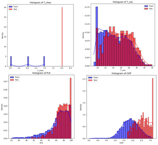
Figure 5.
Histograms of variables Tchw,s, Tcw,s, PLR, and COP in training and testing tasks.
Overall, the distributions of the Tcw,s, PLR, and COP variables are basically similar in the training and testing tasks. The Tchw,s data distribution is consistent with the expected task data division. The situations of these three variables support the model’s rapid adaptation to the testing task through meta-learning. PLR and COP both exhibit peak phenomena in the testing task, which may reflect subtle differences in sample size or data distribution.
Figure 6 shows the correlations between the variables Tchw,s, Tcw,s, PLR, and COP in the training and testing datasets, with correlation coefficients represented by varying shades of color, ranging from −1.00 to 1.00. In the training dataset, the correlation coefficient between Tchw,s and COP is 0.52, indicating a moderate positive correlation; Tcw,s has a correlation coefficient of 0.57 with PLR, indicating a moderate positive correlation; Tcw,s has a correlation coefficient of −0.47 with COP, indicating a moderate negative correlation; PLR has a correlation coefficient of 0.26 with COP, indicating a weak positive correlation. In the test set, the correlation coefficient between Tcw,s and PLR decreases to 0.46; Tcw,s and COP had a strong negative correlation with a correlation coefficient of −0.92; PLR and COP had a weak negative correlation with a correlation coefficient of −0.12. There were no significant differences in the correlation patterns between the training and test sets, which facilitates model transfer learning.
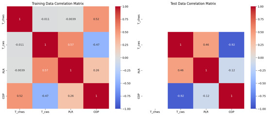
Figure 6.
Heat map of correlation matrices for variables Tchw,s, Tcw,s, PLR, and COP in training and testing tasks.
The PCA scatter plot (Figure 7) shows the distribution of the training set (blue dots) and test set (red dots) in the principal component space (PC1 and PC2), capturing the overall structure and variability of the data. Data points are densely distributed in the central region with PC1 approximately ranging from −20 to 20 and PC2 approximately ranging from −2 to 4, exhibiting a diagonal trend and forming a triangular or fan-shaped distribution overall, indicating that PC1 and PC2 capture the main variability. The training set and test set overlap in the central region but show separation in the peripheral regions, such as high PC1 and high PC2 values. For example, the red points of the test set are more dispersed in the positive PC1 and positive PC2 region (i.e., the upper-right quadrant), while the blue points of the training set are more uniformly distributed in the negative PC1 and negative PC2 region (i.e., the lower-left quadrant).
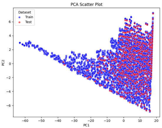
Figure 7.
PCA scatter plot of variables Tchw,s, Tcw,s, PLR, and COP on training and testing tasks.
Overlapping regions indicate similarities between the training set and test set in the principal component space, potentially reflecting shared feature patterns. For example, the low-value regions of Tcw,s may contribute to the overlap in the central region. Overlapping regions support the model’s ability to rapidly adapt to test tasks through meta-learning, indicating task similarities that facilitate the sharing of initialization parameters. Separated regions (such as the unique distribution of the test set in high PC1 and high PC2 regions) suggest the uniqueness of the test task, which may be related to high-value regions of Tchw,s, PLR, or COP. Separated regions indicate that the model needs to adapt to the uniqueness of the test task through fine-tuning, which may require optimizing initialization parameters or adjusting inner loop/outer loop update rules to quickly adapt to these differences with a small number of samples.
3.1.2. Analysis of Experimental Results
During the experiment, the hyperparameters of the MAML-based chiller energy efficiency model were optimized using grid search to achieve good training results. The hyperparameter optimization results are shown in Table 3.
Table 3.
MAML training process hyperparameters.
By investigating the changes in the number of fine-tuned data (training set) for each test task and comparing the performance of the MAML and Standard (MLP) models on the test set for each test task, as shown in Figure 8, it can be seen that the MSE, MAE, and MRE all show a gradual increase as the number of fine-tuned data decreases. The R2 shows a slight overall downward trend and is close to 1.
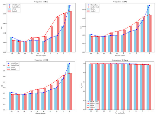
Figure 8.
Comparison of performance metrics between MAML and standard models as fine-tuned data changes.
When the number of fine-tuning iterations is 300, the MSE, MAE, and MRE of the MAML model are greater than those of the Standard model, indicating that the MAML model performs worse than the Standard model on the test set at this point; until the number of fine-tuning iterations ranges from 200 to 5, the MSE, MAE, and MRE of the MAML model are almost all smaller than those of the Standard model, indicating that the MAML model performs better on the test set when the number of fine-tuning iterations is smaller; When the number of fine-tuning iterations is 4, the MSE, MAE, and MRE of the MAML model are greater than those of the Standard model. This may be because with fewer fine-tuning iterations, the MAML model is not sufficiently fine-tuned for the test task, resulting in the meta-model trained on the training task not adapting to the data in the test task, thus leading to poorer performance.
Analysis of the trends in MSE, MAE, and MRE in Figure 8 shows that when the number of fine-tuned parameters ranges from 200 to 5, the MAML model exhibits a more stable trend in metric changes compared to the Standard model, which experiences greater metric fluctuations. This indicates that MAML demonstrates certain advantages in small-sample learning and is well-suited for scenarios with scarce data.
When the number of fine-tuning parameters is set to 5, the comparison plots of the true values and predicted values of the COP, as well as the relative error comparison plots, for the MAML and Standard models on the test set are shown in Figure 9. As can be seen from the figure, the MAML model’s predicted values are generally closer to the true values, with smaller relative errors, and the RE are mostly kept below 3%, meeting the requirements of engineering practice. It can be concluded that the MAML-improved chiller energy efficiency model achieves satisfactory model accuracy with only a small amount of data under different operating conditions of the same equipment with varying chilled water temperatures (Tchw,s). The following section continues to explore the performance of the MAML-improved chiller energy efficiency model in data-scarce scenarios under cross-equipment operating conditions.
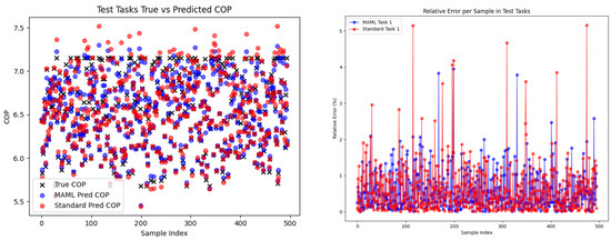
Figure 9.
Error performance of MAML and standard models under different operating conditions on the same device.
3.2. Performance Analysis of the MAML Energy Efficiency Model Under Cross-Device Scenarios (Same Equipment Type) Operating Conditions
In this section, the historical operational data of Chiller Unit 1 and Chiller Unit 2 are utilized as the training dataset. Specifically, the dataset from Chiller Unit 1 serves as the training task ΦA, while the dataset from Chiller Unit 2 serves as the testing task ΦB. Both the training and testing tasks are further subdivided into a training set (Dtrain) and a test set (Dtest). The split ratio can be adjusted based on the training objectives and model predictive performance; in this case, a 7:3 ratio for Dtrain to Dtest is adopted within training task ΦA.
The dataset configuration used for training both the MAML and Standard models is similar to that described in Section 3.1. After partitioning the task data, preprocessing procedures are applied. This includes K-means clustering for sampling, deduplication, missing value imputation, Z-score normalization, and comparative analysis of the statistical distributions between the training and testing tasks to ensure data cleanliness. Following these steps, the processed training task dataset comprises 1000 samples, and the testing task dataset likewise consists of 1000 samples. During experimentation, the hyperparameters of the MAML-based chiller energy efficiency model are optimized via grid search to achieve robust training performance.
The dataset from Chiller Unit 1 serves as the training task ΦA, while the dataset from Chiller Unit 2 functions as the testing task ΦB. Both the training and testing tasks partition into their respective Dtrain and Dtest. The models are solved using the algorithm described in Section 2. When the volume of fine-tuning data is set to 500 samples, the comparative training loss results for the MAML and Standard models are shown in Figure 10. Results show that the loss of the Standard model decreases to a value of 1 and then plateaus, accompanied by a large relative error. This indicates that the model training fails to find a gradient descent direction beyond a certain point. Analysis identifies the primary reason: the training dataset for this model comprises the complete operational data of Chiller Unit 1 and a subset of the operational data from Chiller Unit 2. Data processing reveals that the characteristics of the energy efficiency curves differ between Chiller Unit 1 and Chiller Unit 2. A single MLP neural network struggles to adapt simultaneously to these two datasets with significantly different distributions.
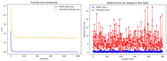
Figure 10.
Comparison of training loss and relative error between MAML and standard models.
This study investigates the impact of varying the number of fine-tuning data points on the performance of the MAML and Standard (MLP) models, as evaluated on the test set of the testing task. As shown in Figure 11, the MSE, MAE, and MRE exhibit a gradual increasing trend as the number of fine-tuning samples decreases, while the R2 shows a slight overall decreasing trend.
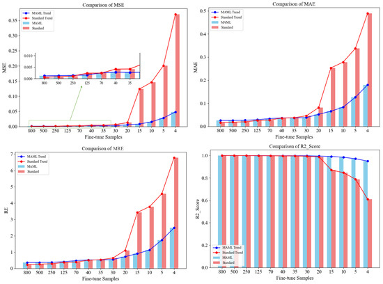
Figure 11.
Comparison of performance metrics between MAML and standard models with varying fine-tuning data.
When the number of fine-tuning samples ranges from 800 to 125, the MSE, MAE, and MRE of the MAML model are higher than those of the Standard model. This indicates that the predictive performance of the MAML model on the test set is inferior to that of the Standard model within this data range. Conversely, when the number of fine-tuning samples is reduced to between 40 and 4, the MSE, MAE, and MRE of the MAML model become lower than those of the Standard model. This demonstrates that the MAML model achieves superior predictive performance on the test set with limited fine-tuning data. Analysis of the trends in MSE, MAE, and MRE in Figure 11 reveals that as the number of fine-tuning samples decreases from 20 to 4, the performance metrics of the MAML model change more steadily compared to the Standard model, whose error metrics exhibit a sharp increase. This result underscores the advantage of MAML in few-shot learning scenarios, highlighting its suitability for applications with scarce data.
Figure 12 presents a comparison between the actual and predicted COP values on the test set, along with their relative errors, for both the MAML and Standard models when the number of fine-tuning samples is 4. As shown in Figure 12, the overall predictions of the MAML model align more closely with the actual values and exhibit smaller relative errors. Furthermore, the RE are consistently maintained within 5%, satisfying the requirements for engineering applications. It can be concluded that the MAML-improved chiller energy efficiency model achieves satisfactory accuracy in cross-device (same type) scenarios with just 4 or more fine-tuning samples. The following section continues to investigate the performance of the MAML-enhanced chiller energy efficiency model under cross-device-type operating conditions in data-scarce scenarios.
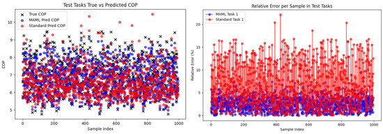
Figure 12.
Error performance of MAML and standard models under cross-device scenarios (same equipment type) operating conditions.
3.3. Analysis of Data Collection Reduction and Practical Energy-Saving Benefits
As evidenced by the experimental results, the MAML model’s rapid adaptation capability enables it to achieve performance comparable to the Standard model using significantly less data on new device datasets. Specifically, under varying operating conditions on the same device, the MAML model requires only 5 fine-tuning data points to achieve a model RE below 3%, while the Standard model requires 10 data points—representing a 50% reduction in data requirement. In cross-device scenarios (with identical equipment types), the MAML model achieves RE below 5% with merely 4 fine-tuning data points, compared to approximately 15 points needed by the Standard model, resulting in a 73% data reduction. The improvement in prediction accuracy (RE within 3–5%) is not merely a statistical gain but translates directly into enhanced potential for operational energy savings. To quantify this, a brief analysis is conducted based on the chiller units studied. Consider Chiller Unit 1 (rated cooling capacity: 4920.3 kW) operating under a typical partial load condition (e.g., PLR = 80%) for a full cooling season (assumed to be 120 days, 10 h per day). The seasonal cooling energy output (Qseason) is 4,723,488 kWh. The seasonal electricity consumption depends on the average COP. Assuming an average COP of 5.0 without optimization and a conservative estimate that accurate predictive modeling can facilitate control strategies leading to a mere 1% improvement in operational COP (from 5.0 to 5.05) [23,24], the resultant seasonal energy saving (ΔEseason) is 9354 kWh. Therefore, the MAML model’s ability to achieve high accuracy with minimal data not only reduces the data acquisition cost but also secures the energy-saving payoff of subsequent optimization by providing a reliable performance model.
For energy retrofit projects or new construction projects involving central air-conditioning systems, deploying intelligent operational strategies typically requires substantial historical operational data for support. The implementation of the MAML-enhanced equipment model reduces this dependency on large datasets. By leveraging minimal data, the system can rapidly characterize equipment performance and deploy optimization strategies. This capability facilitates quicker precise control of equipment, ultimately leading to improved energy savings and reduced consumption.
4. Conclusions
This study employs the MAML algorithm, training a universal meta-model through its bi-level optimization mechanism. In the inner loop, task-specific parameters are rapidly adapted using support set data, while the outer loop optimizes initial parameters to enhance cross-task adaptability. The experimental design encompasses two operating scenarios: varying conditions on the same device and cross-device scenarios (same equipment type)—with performance comparisons made between MAML and Standard models. Data preprocessing included K-means clustering sampling and Z-score normalization, while evaluation metrics comprised MSE, MAE, MRE, and R2.
Experimental results demonstrate that the MAML model consistently outperforms standard models in few-shot learning across all three scenarios. For varying conditions on the same device, only 5 fine-tuning data points are required to achieve RE below 3%. In cross-device scenarios (same equipment type), RE remains below 5% with just 4 data points. Compared to Standard models, MAML significantly reduces data requirements (achieving reductions of 50% and 73%, respectively) and maintains more stable prediction performance as fine-tuning data decreases, highlighting its advantage in data-scarce environments.
This study enhances the generalization capability and adaptability of chiller energy efficiency models through meta-learning, providing an efficient solution for intelligent management and energy optimization in central air-conditioning systems. Its practical applications are mainly reflected in: (1) offering rapid and low-cost equipment modeling and energy-saving potential analysis for existing building energy retrofit projects lacking historical data; (2) accelerating the deployment of digital twin models in new or intelligently upgraded buildings, promoting the early implementation of data-driven optimization strategies; (3) providing a more reliable performance benchmark model for fault detection and diagnosis (FDD) under varying operating conditions or equipment performance drift scenarios; (4) enabling knowledge transfer and scalable energy management across similar building clusters. The theoretical value lies in validating the feasibility of MAML in industrial applications, while the practical value is demonstrated through reduced data collection costs, accelerated model deployment, and optimized operational strategies. It should be noted that the primary limitation of this study lies in the fact that validation is based solely on operational data from two centrifugal chillers within a single building. Although the results demonstrate a significant improvement in few-shot learning performance, the generalizability of the proposed MAML model requires further verification. Future work will focus on expanding the scale of validation by applying the framework to larger, publicly available datasets encompassing various types and sizes of chiller units. Additionally, we will explore the transferability of the meta-learning approach to other critical components of heating ventilation air conditioning (HVAC) systems, such as water pumps and cooling towers. These findings establish a foundation for rapid model construction and optimization of equipment under complex operating conditions and demonstrate significant potential for the practical engineering applications outlined above.
Author Contributions
S.G.: Conceptualization, Data curation, Formal analysis, Investigation, Writing—original draft. G.P.: Writing—original draft, Investigation, Data curation, Funding acquisition, Supervision. S.C.: Methodology, Software, Project administration, Validation, Visualization. J.J.: Project administration, Resources, Software, Visualization, Supervision. Z.D.: Data curation, Investigation, Formal analysis, Resources, Writing—original draft, Validation. Z.C.: Funding acquisition, Project administration, Resources, Supervision, Writing—review & editing. All authors have read and agreed to the published version of the manuscript.
Funding
This work was supported by Zhejiang Province Science and Technology Program Project “Key Technology Research and Application of Active and Passive Composite Cooling Systems for Data Centers” (2023C01122) and the Big Data Center of Southeast University for providing the facility support on the numerical calculations in this paper.
Data Availability Statement
The original contributions presented in this study are included in the article. Further inquiries can be directed to the corresponding author(s).
Conflicts of Interest
Author Guiping Peng was employed by the company Huaxin Consulting Co. Ltd. Author Shiheng Chai was employed by the company Huaxin Consulting Co. Ltd. Author Jiwei Jia was employed by the company China Telecom Co. Ltd. The remaining authors declare that the research was conducted in the absence of any commercial or financial relationships that could be construed as a potential conflict of interest.
Abbreviations
The following abbreviations are used in this manuscript:
| AdamW | Adam with Weight Decay |
| ANNs | Artificial neural networks |
| COP | Coefficient of Performance (-) |
| Dtrain | Training sets |
| Dtest | Testing sets |
| FDD | Fault detection and diagnosis |
| HVAC | Heating ventilation air conditioning |
| ITEROuter | The number of outer loop iterations |
| ITERInner | The number of inner loop iterations |
| MAE | Mean absolute error (-) |
| MAML | Model-agnostic meta-learning |
| MLP | Multilayer perceptron |
| MRE | Mean relative error (%) |
| MSE | Mean squared error (-) |
| PCA | Principal components analysis |
| PLR | Part load ratio (%) |
| R2 | Coefficient of determination (-) |
| RE | Relative error (%) |
| RF | Random forests |
| RMSE | Root mean square error (-) |
| SVR | Support vector regression |
| Tcw,s | Cooling water supply temperature (°C) |
| Tchw,s | Chilled water supply temperature (°C) |
| yi | The true value of the i-th sample |
| α | The outer loop learning rate |
| β | The inner loop learning rate |
| ΦA | Training tasks |
| ΦB | Testing tasks |
References
- Wang, Z.; Pang, Z. Adaptive transfer reinforcement learning (TRL) for cooling water systems with uniform agent design and multi-agent coordination. Energy Build. 2025, 345, 116071. [Google Scholar] [CrossRef]
- Afroz, Z.; Shafiullah, G.M.; Urmee, T.; Higgins, G. Modeling techniques used in building HVAC control systems: A review. Renew. Sustain. Energy Rev. 2018, 83, 64–84. [Google Scholar] [CrossRef]
- Li, Q.; Zhou, Y.; Wei, F.; Long, Z.; Li, J.; Ma, Y.; Zhou, G.; Liu, J.; Yan, P.; Yu, D. Harmonizing comfort and energy: A multi-objective framework for central air conditioning systems. Energy Convers. Manag. 2024, 314, 118651. [Google Scholar] [CrossRef]
- Thangavelu, S.R.; Myat, A.; Khambadkone, A. Energy optimization methodology of multi-chiller plant in commercial buildings. Energy 2017, 123, 64–76. [Google Scholar] [CrossRef]
- Wei, X.; Li, N.; Peng, J.; Cheng, J.; Hu, J.; Wang, M. Modeling and Optimization of a CoolingTower-Assisted Heat Pump System. Energies 2017, 10, 733. [Google Scholar] [CrossRef]
- Pan, C.; Li, Y. Nonlinear model predictive control of chiller plant demand response with Koopman bilinear model and Krylov-subspace model reduction. Control Eng. Pract. 2024, 147, 105936. [Google Scholar] [CrossRef]
- Serale, G.; Fiorentini, M.; Capozzoli, A.; Bernardini, D.; Bemporad, A. Model Predictive Control (MPC) for Enhancing Building and HVAC System Energy Efficiency: Problem Formulation, Applications and Opportunities. Energies 2018, 11, 631. [Google Scholar] [CrossRef]
- Shahcheraghian, A.; Madani, H.; Ilinca, A. From White to Black-Box Models: A Review of Simulation Tools for Building Energy Management and Their Application in Consulting Practices. Energies 2024, 17, 376. [Google Scholar] [CrossRef]
- Chen, S.; Ding, P.; Zhou, G.; Zhou, X.; Li, J.; Wang, L.; Wu, H.; Fan, C.; Li, J. A novel machine learning-based model predictive control framework for improving the energy efficiency of air-conditioning systems. Energy Build. 2023, 294, 113258. [Google Scholar] [CrossRef]
- Afram, A.; Janabi-Sharifi, F.; Fung, A.S.; Raahemifar, K. Artificial neural network (ANN) based model predictive control (MPC) and optimization of HVAC systems: A state of the art review and case study of a residential HVAC system. Energy Build. 2017, 141, 96–113. [Google Scholar] [CrossRef]
- Kim, J.-H.; Seong, N.-C.; Choi, W. Forecasting the Energy Consumption of an Actual Air Handling Unit and Absorption Chiller Using ANN Models. Energies 2020, 13, 4361. [Google Scholar] [CrossRef]
- Cai, W.; Wen, X.; Li, C.; Shao, J.; Xu, J. Predicting the energy consumption in buildings using the optimized support vector regression model. Energy 2023, 273, 127188. [Google Scholar] [CrossRef]
- Tang, R.; Fan, C.; Zeng, F.; Feng, W. Data-driven model predictive control for power demand management and fast demand response of commercial buildings using support vector regression. Build. Simul. 2022, 15, 317–331. [Google Scholar] [CrossRef]
- Smarra, F.; Jain, A.; de Rubeis, T.; Ambrosini, D.; D’Innocenzo, A.; Mangharam, R. Data-driven model predictive control using random forests for building energy optimization and climate control. Appl. Energy 2018, 226, 1252–1272. [Google Scholar] [CrossRef]
- Lu, S.; Li, Q.; Bai, L.; Wang, R. Performance predictions of ground source heat pump system based on random forest and back propagation neural network models. Energy Convers. Manag. 2019, 197, 111864. [Google Scholar] [CrossRef]
- Zhang, H.; Li, Z.; Fan, X.; Duan, D.; Zheng, W. Air-conditioning load characteristics and grey box predicting model in subway stations. J. Build. Eng. 2024, 91, 109656. [Google Scholar] [CrossRef]
- Li, Z.; Guo, J.; Gao, X.; Yang, X.; He, Y.-L. A multi-strategy improved sparrow search algorithm of large-scale refrigeration system: Optimal loading distribution of chillers. Appl. Energy 2023, 349, 121623. [Google Scholar] [CrossRef]
- Jiang, S.; Hui, H.; Song, Y. Credible demand response capacity evaluation for building HVAC systems based on grey-box models. Appl. Energy 2025, 395, 126144. [Google Scholar] [CrossRef]
- Sarmas, E.; Spiliotis, E.; Marinakis, V.; Koutselis, T.; Doukas, H. A meta-learning classification model for supporting decisions on energy efficiency investments. Energy Build. 2022, 258, 111836. [Google Scholar] [CrossRef]
- Kumkam, S.; Trinuruk, P.; Chaiwiwatworakul, P.; Rakkwamsuk, P.; Bangviwat, A. Study on Adaptation of Model-Agnostic Meta-Learning Integrated Deep Q-Learning for HVAC Control. In Proceedings of the 2024 IEEE International Smart Cities Conference (ISC2), Pattaya City, Thailand, 29 October–1 November 2024; pp. 1–6. [Google Scholar]
- Xiong, J.; Peng, T.; Tao, Z.; Zhang, C.; Song, S.; Nazir, M.S. A dual-scale deep learning model based on ELM-BiLSTM and improved reptile search algorithm for wind power prediction. Energy 2023, 266, 126419. [Google Scholar] [CrossRef]
- Trautman, N.; Razban, A.; Chen, J. Overall chilled water system energy consumption modeling and optimization. Appl. Energy 2021, 299, 117166. [Google Scholar] [CrossRef]
- Wu, S.; Yang, P.; Chen, G.; Wang, Z. Evaluating seasonal chiller performance using operational data. Appl. Energy 2025, 377, 124377. [Google Scholar] [CrossRef]
- Xue, Q.; Jin, X.; Jia, Z.; Lyu, Y.; Du, Z. Optimal control strategy of multiple chiller system based on background knowledge graph. Appl. Energy 2024, 375, 124132. [Google Scholar] [CrossRef]
Disclaimer/Publisher’s Note: The statements, opinions and data contained in all publications are solely those of the individual author(s) and contributor(s) and not of MDPI and/or the editor(s). MDPI and/or the editor(s) disclaim responsibility for any injury to people or property resulting from any ideas, methods, instructions or products referred to in the content. |
© 2025 by the authors. Licensee MDPI, Basel, Switzerland. This article is an open access article distributed under the terms and conditions of the Creative Commons Attribution (CC BY) license (https://creativecommons.org/licenses/by/4.0/).