1. Introduction
The pollution of the environment by combustion products is one of the main global problems. The most dangerous gasses are carbon dioxide, carbon monoxide, and NOx gasses. Gas purification from CO
2 and other impurities using amine extraction technology is rather popular and effective [
1]. Despite this, the most effective method of removing NOx gasses is catalytic purification using additional reagents [
2,
3,
4]. In this case, ammonia or ammonia solution in water (as such a chemical reagent) is fed into the flue gasses, due to the toxicity and corrosive activity of pure ammonia. In addition, urea can be used as a reagent (SCR cleaning system). Chemical interaction leads to NOx compounds being reduced to safe N
2 and H
2O on the catalyst [
5,
6].
Analysis of the operation of DeNOx purification units shows that the quality of this purification is significantly affected not only by the characteristics of the catalyst and the kinetics of the chemical process but also by the final quality of the reagent distribution in the flue gas flow before the catalyst. Poor distribution leads to low ammonia content in part of the flow and NOx gas breakthrough during the purification process. Therefore, high-quality mixing and distribution of components throughout the entire gas volume is a must when operating DeNOx systems.
Various static mixers are used to ensure the required parameters of high-quality mixing [
7,
8,
9,
10,
11,
12]. They allow the creation of turbulent vortices in the flow, as a result of which the homogeneity of the reagent is significantly increased.
Analyses of static mixers of various designs used for DeNOx units and their classification are given in [
7,
8,
9,
10,
11,
12]. Hollow mixers with and without nozzles are used in industry. In [
7], it is noted that low hydraulic resistance seems to be their only advantage. Mixers with several segment partitions that block part of the mixer cross-section are used in industry [
7]. Such partitions significantly increase hydraulic resistance, but the mixing quality in the mixer is not high enough. Examples of different types of mixers are shown in
Figure 1.
The highest mixing quality is achieved while using mixers with plate turbulators—blades (curved, located along the contour, or fan-shaped straight plates)—as well as with filling—packing (regular or irregular). The best mixing quality is achieved in mixers with packed bodies as filler. The cost and hydraulic resistance of such mixers are higher. Mixers with regular packing have lower hydraulic resistance and rather worse distribution quality. Due to the high cost, the use of such mixers is not justified. Turbulent static mixers with blades also allow achieve good mixing quality in small mixing areas (about 3–5 mixer diameters) [
10,
11]. Considering the low cost of the selected type of mixers, they are quite common. The most significant disadvantages of all the listed types of mixers, providing the greatest uniformity of mixing, are the significant price and complexity of the design.
The type and design of each type of mixer have a significant impact on the mixing process [
10,
11], especially in paddle mixers. The most convincing test data show that direct experimental study on the physical models of mixers is the preferred research method. However, it is possible to use numerical modeling for these purposes in order to save time, significant resources, and production space [
3,
4,
5,
6].
The analysis shows that most industrial mixers are quite expensive and difficult to maintain; in particular, these are mixers with a nozzle or that use nozzles. It is known that when exposed to high temperatures, these types of mixers may not work correctly or even break. Using paddle mixers can solve these problems. Thus, the main goals of this article can be determined as follows:
- -
The development of a paddle mixer with low metal consumption that provides an acceptable mixing quality;
- -
The numerical modeling and analysis of its operation, with confirmation of the expected operating characteristics in a given load range;
- -
The development and creation of an experimental model in real production
- -
The comparison of key parameters of the mixer operation, obtained by calculation and experiment.
2. Model Description
The static mixer presented in this work refers to blade mixers with a central feed of ammonia. Its design and operating principle are similar to those described in works [
7,
11,
12] but differ in shape, blade arrangement, and reagent feed method.
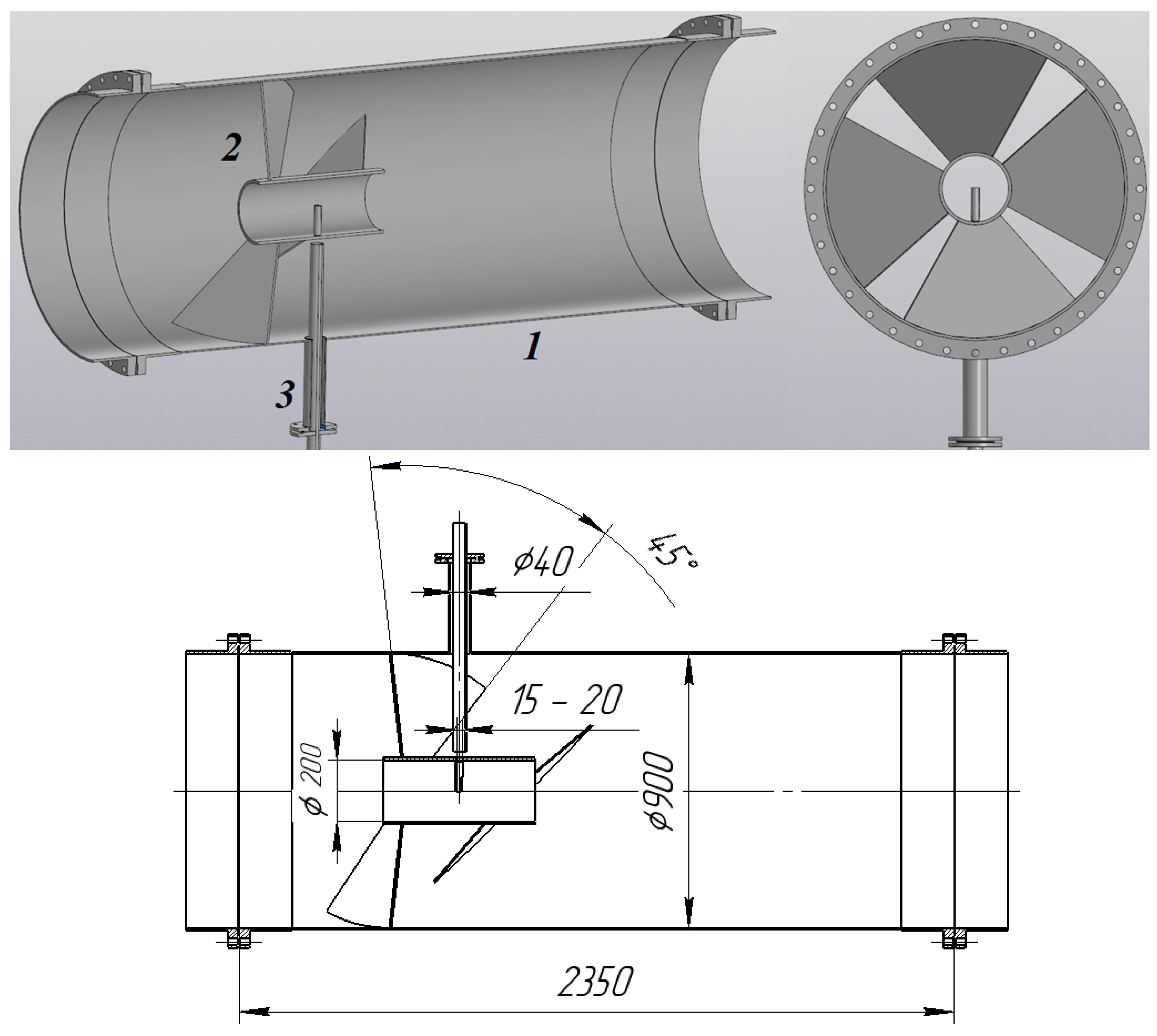
The developed 3D model of the mixer is shown in
Figure 2.
The mixer consists of an outer pipe (1), with a diameter of D = 900 mm, a swirler (2) with inclined blades (45° to the mixer axis), and a central channel for ammonia solution feeding (3). The outer pipe has flanges for fastening to the installation pipeline. Ammonia solution is fed through the channel (3). In this work, the feed channel was considered to be a pipe in which the ammonia solution is heated and then evaporates into the flue gas flow. The outlet from the channel is located exactly in the center of the swirler (2). The diameter of the channel (3) is 15 mm. The mixer has 2 rows of inclined blades, allowing for the creation of four turbulent flows directed in different directions, mixing with each other.
The composition of gasses is rather complex. Thus, we assume that the flue gas is a homogeneous medium in which the properties are distributed equally throughout the volume to obtain a picture of the distribution of components. We also assume that the composition of the gas is determined based on nitrogen, oxygen, carbon dioxide, and other impurities not exceeding 5% of the total amount of nitrogen, carbon dioxide, and oxygen.
The design shown differs from the previously considered mixers with blades. In particular, the blades are arranged in two rows, so that they form four counter flows that are mixed simultaneously. The feed is carried out in the center of such a flow, which leads to the continuous distribution of the component throughout the mixing zone.
Moreover, the supplied ammonia solution is clearly decomposed into water (H2O) and ammonia (NH3). The interval of the conducted studies on the consumption of flue gasses is G = 17,500–35,000 kg/h, according to experimental data. Lower gas consumption will have a proportionally lower mass velocity of the components. The mixing process will take place at a temperature of 450 °C; it is assumed that the mixture of ammonia with water vapor is already supplied at this temperature as gas. The gas phase (flue gasses) also initially contains water xH2O = 7.33/35,000 = 0.00021 (mass). Since the main objective was to study the distribution of ammonia in the flue gas flow, the specified water content was not taken into account. When setting the initial concentration xH2O = 0.00021 during the simulation, the final distribution of the target component does not change.
One of the most important characteristics of the mixer is the homogeneity of the composition after mixing the components. The literature traditionally uses a value that takes into account the average deviation from the average concentration in the section—
Cov [
9,
11,
12,
13]. In addition, the inverse value can be used, taking into account the symmetry of the deviation from the average value—the homogeneity parameter UI (Uniformity Index) or γ [
7,
10,
14,
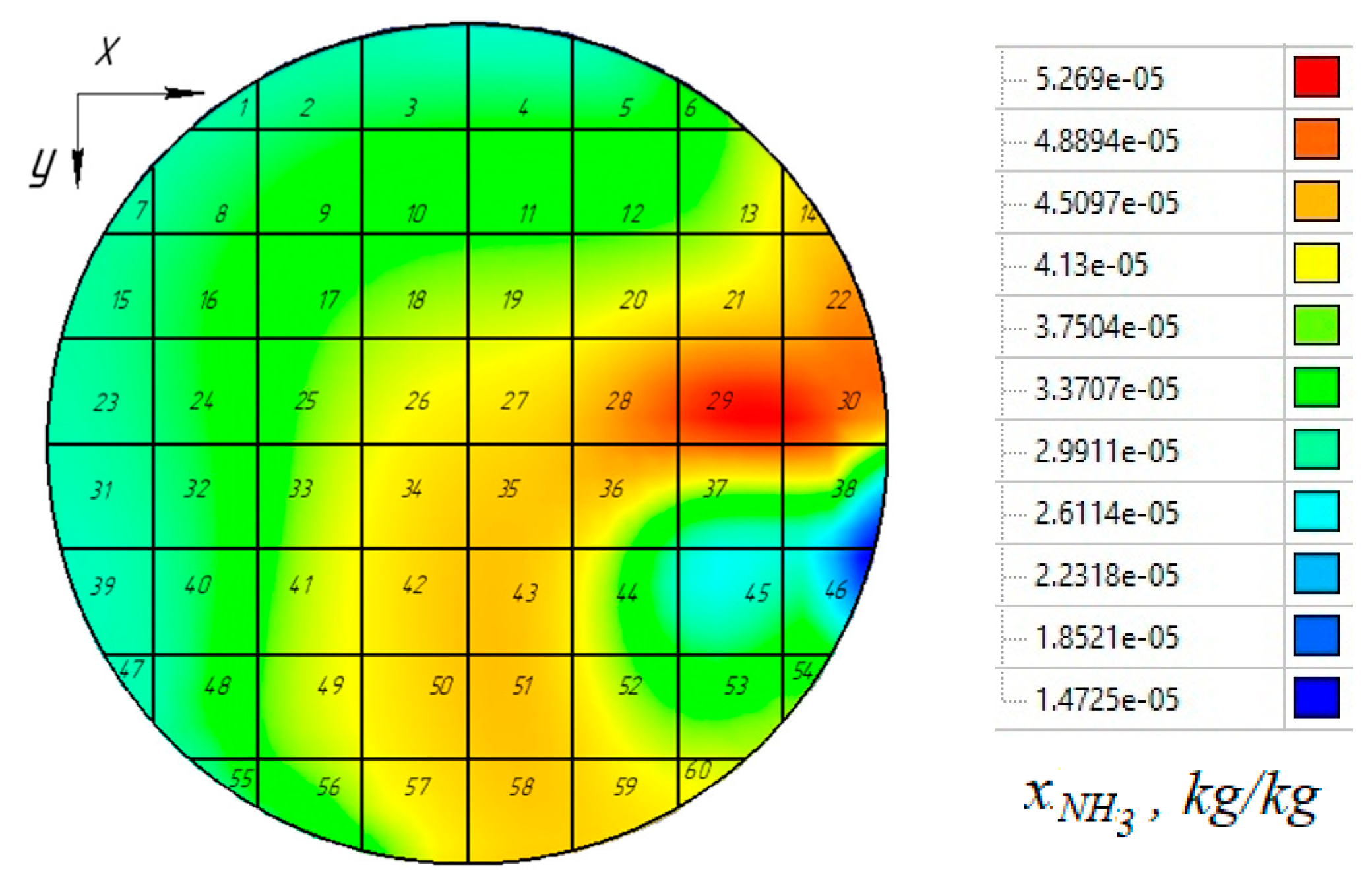
15]. To carry out the calculation according to the given indicators in the mixer section, the section itself is divided into several cells in this work: the number of cells
n = 60. An example of the division into cells is shown in
Figure 3.
It is proposed to use
Cov as the basic parameter determining the homogeneity of the distribution, which (according to [
11,
12]) can be determined as
where
xi—the current average concentration in the cell;
—the total average concentration in the mixer section. It can be determined by [
14] that
n is the number of cells in the section.
Also, in a number of works (for example, in [
15]), the
UI parameter is used:
The
UI parameter is generally similar to
Cov and the inverse value—the correspondence of the obtained concentrations to its average value in the section. In this case (according to [
14]), the average concentration in a given section is determined using the area of the sectors Ai (m
2) and the total area of the section A (m
2), as shown in
Figure 4.
The considered indicators are not universal and do not allow us to fully assess the degree of unevenness of the concentration distribution in the flue gas flow. Therefore, the value of the effective mixing length is used (calculated using the ratio of this length and the diameter of the mixer L/D) to compare the operation of mixers. In this case, the value of
Cov = 5% should be achieved in the specified section, according to [
9,
11,
12,
13].
To achieve the goal specified in this work, the following tasks were solved: the determination of the concentration in the sections of the mixer in the load range and determination of Cov and L/D along the length of the mixer from the gas load.
Mathematical (numerical) modeling was chosen as the method for conducting this study. The model was implemented using the Navier–Stokes and Fick equations, as well as a number of empirical modifications (for example, the turbulence model). The equations were solved using a numerical algorithm. The Flow Vision 3.14 package (TESIS LLC.) was used to solve this problem. Parametric 3D models were used to implement the algorithm, and the complex of calculations allowed us to identify patterns of gas movement and mass transfer. As a result, with the use of built-in models numerically solving differential equations, it is possible to obtain the distribution of parameters such as temperature, velocity, pressure, component concentration, and others. Similar methods have already been used, for example, in [
6,
10,
13,
14,
15,
16,
17]. The motion of complex swirling flows was also studied in works [
18,
19].
The simulation resulted in the velocity distribution and ammonia concentrations across the distributor cross-section and determined
Cov in a section of up to 5 m, similarly to works [
9,
11,
12,
13]. The object of this study was a three-dimensional model of the mixer. The geometric model represents the space occupied by the gas when moving inside the pipe. In this case, the feed tube and blades were excluded from the volume, limiting the volume of gas. The model shown in
Figure 4 was created as the main three-dimensional model of the experimental area.
The calculation area had a mixing section length of Lmix = 5 m (which corresponds to 5.5 D of the mixer), which is not shown in full in
Figure 5. The setup of the calculation area of the mixer in the Flow Vision 3.14 program had a number of features and assumptions, which are indicated below:
1. The flue gas flow rate was set in the range G = 17,500–35,000 kg/h and was installed before the mixer. The standard mass velocity set for the flue gas flow was W1 = 15.3–7.65 kg/(m
2 s). The standard mass velocity of ammonia water was W2 = 7.8–3.9 kg/(m
2 s). The concentration of the aqueous NH
4(OH) solution was 25%. Its flow was set as the gas phase flow rate, assuming that the liquid would evaporate. The final concentration of ammonia in water vapor was xNH
3 = 12.1%. The direction of the flue gas flow was along the axis (axially), and the direction of ammonia water flow was in the transverse direction (radially), normally corresponding to the sections. The main parameters of the experiment are given in
Table 1.
2. The wall temperature (the boundary of the calculation area) was assumed to be constant and was 450 °C. The coolant temperature at the module inlet was 450 °C. The initial calculation conditions were also at 450 °C. Heat exchange with the environment was not taken into account due to the presence of insulation. This is confirmed by minor temperature fluctuations throughout the pipeline section (10–15 °C) at the operating DeNOx installation.
3. Sufficient convergence on the grid was achieved. The minimum number of cells of the main grid along the mixer was 130, across 35 × 35. Adaptations were also used.
4. The gravity vector was oriented vertically from top to bottom (opposite the Y axis and the direction of the ammonia water supply), which corresponded to the installation of the mixer on the unit.
5. The k-ε model was chosen for describing the turbulence. The applicability of this model in most studies of mixers is proved in [
13,
14,
15,
16,
17]. This model is universal and allows for rapid convergence in calculations. This differential turbulence model has two unknowns. Therefore, two additional transfer equations are used to account for average pulsation characteristics. This model also takes into account the pressure gradient in the wall functions.
The standard
k-ε model includes the following dependencies for the turbulent kinetic energy
k (4) and the energy dissipation rate
ε (5), written along one of the coordinates [
15]:
where
ρ—flow density kg/m
3;
xi—current coordinate, m;
t—time, s;
ui—flow rate, m/s;
μ—viscosity, Pa·s;
μt—turbulent viscosity, Pa·s;
σε—the turbulent Prandtl number for ε (σε = 1.30);
Gk—generation of turbulent kinetic energy;
σk—the turbulent Prandtl number for k;
C1ε, C2ε—coefficients for the model (C1ε = 1.44, C2ε =1.92).
6. The coolant is discharged through the side section of the mixer, located on the opposite side from the input. The boundary condition “free outlet” (zero outlet pressure value) was selected.
3. Model Verification
The obtained modeling results were verified using data obtained at the operating DeNOx plant using the mixer of the developed design. The real mixer located at Technopark Real-Invest LLC is shown in
Figure 5.
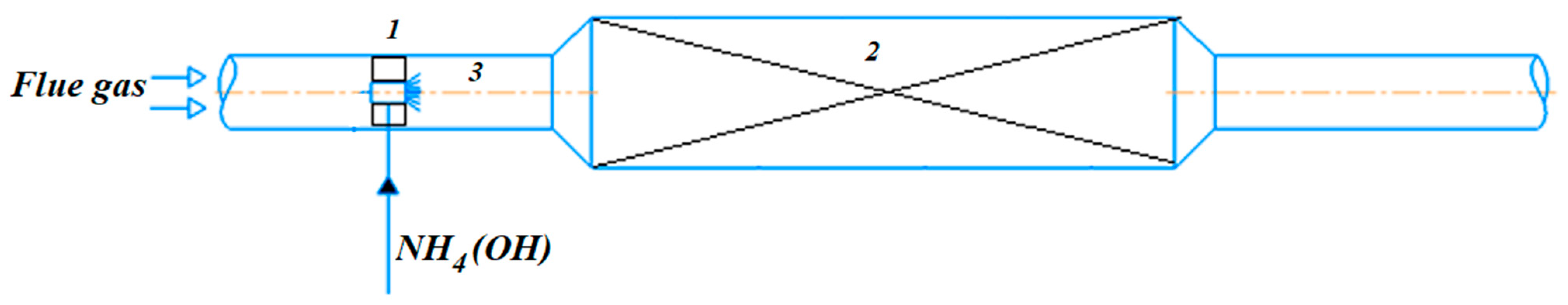
The basic operation diagram of the mixer is shown in
Figure 6.
The gas enters the mixing chamber (1) at a temperature of about 450 °C. At the same time, the flow is prepared for mixing—the degree of its turbulence increases locally. An additional reagent (25% solution of ammonia in water), which is used for the chemical neutralization of NOx gasses, is also fed into the mixer. A forced feed of the reagent is used to ensure a uniform distribution of ammonia in the flue gas flow before the catalytic reduction unit (DeNOx unit (2)). After the mixer, the components are dissolved in the flow due to diffusion mixing, which means that a mixing section (pos. 3) is provided after the mixer. After equalizing the reagent concentrations, the flue gas flow enters the catalytic purification unit, where a chemical reaction occurs to convert NOx gasses into harmless compounds [
10].
Linear velocity profiles were determined using an AGM-510 m (NPC Analyteh) and a Pitot tube (NPO ECO-INTECH) at distances of 2.5 m, 4 m, and 5 m from the insertion point. A probe was inserted into the pipe, and the pressure value was recorded, according to which the velocity was then determined.
To confirm the model’s operability, linear concentration profiles were determined using a gas analyzer (GANK-4, channel A) at distances of 2.5 m, 4 m, and 5 m from the point of supply of ammonia to the pipe. A probe was inserted into special nozzles, and the ammonia concentration values were measured.
All measurements were carried out repeatedly, the average values at the nodal points are summarized in graphs.
4. Results of Numerical Simulation
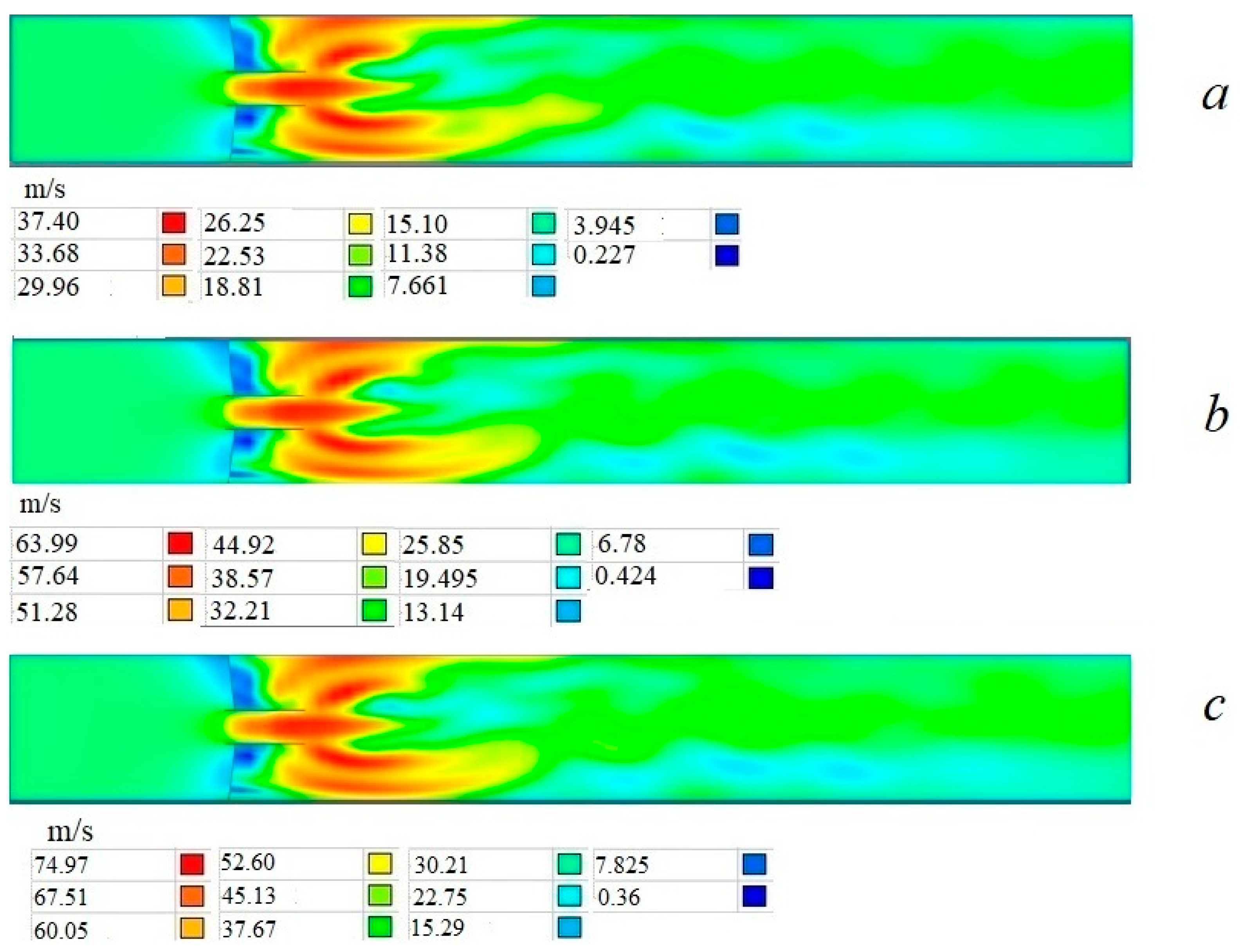
Based on the results of calculations for 50%, 65%, 85%, and 100% of the maximum flue gas flow rate, the Flow Vision 3.14 software package provided data on the distribution of concentrations and velocities. In addition to the specified flow parameters, it was convenient to use the average flue gas velocity (w, m/s) and the Reynolds number determined through w, the equivalent size of the internal diameter of the mixer pipe (D, m), and the kinematic viscosity of gasses at an average temperature (ν, m2/s): Re = w•D/ν. The flue gas velocity variation range was 20–10 m/s. The Reynolds number varied in the range Re = 130,000–260,000.
Figure 7 shows the velocity distributions for different values of flue gas flow rates.
From the figures showing the velocity distribution, it can be established that the movement is carried out along complex trajectories. When the gas passes through the mixer, the flow swirls, and this is reflected in the appearance of a zone with high velocities. The mixer creates volumetric vortices that mix the flow and distribute the ammonia supplied to the central zone. In all cases shown in
Figure 7, the velocity distribution is qualitatively a little different; there are differences in the velocity values.
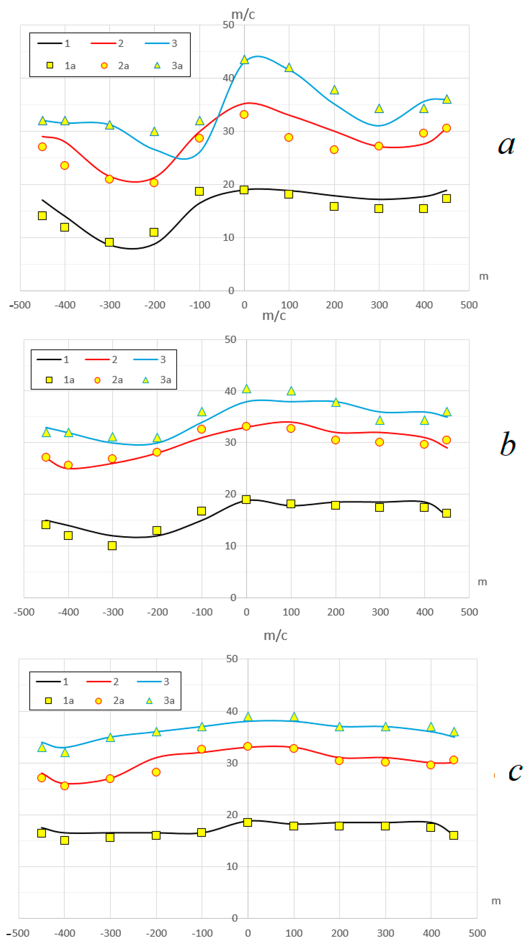
Figure 8 shows a comparison of the theoretical velocity profile and the experimentally obtained values. In analyzing the diagrams, it can be noted that, in general, despite some discrepancies, the shape of the profiles and the velocity values are close and the discrepancy does not exceed 15%. It can also be noted that the experimentally obtained profiles have a smaller spread of values, compared to the profiles obtained using numerical modeling. This can be explained by averaging the readings on the device over the measurement interval, while the theoretically obtained velocities periodically change due to the continuous swirling of the flow.
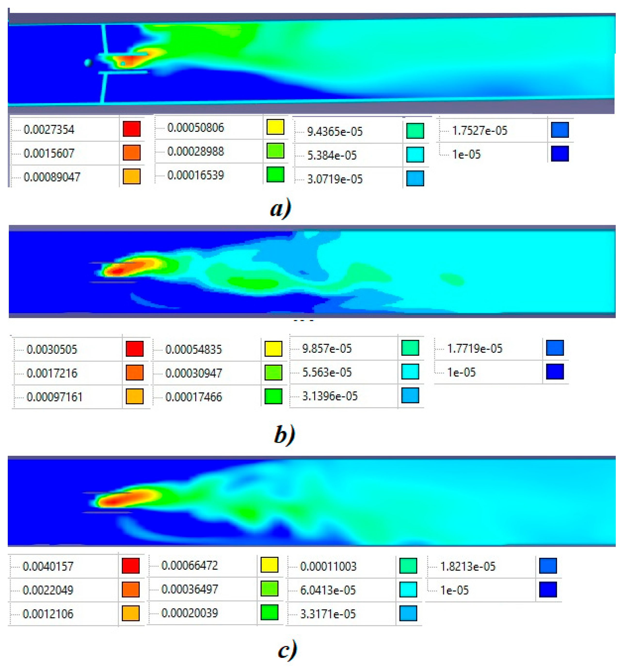
Figure 9 shows the distribution of the NO3 concentration along the central plane along the mixer axis depending on the Reynolds number. For convenience, a logarithmic scale for displaying concentrations was chosen.
In analyzing the presented color contours of the concentration distribution, it can be noted that after 5 m of the flow in the central plane, the concentrations are almost equalized. With a decrease in the gas and reagent consumption, it can be noted that the homogeneity of the flow decreases. At a flue gas flow rate of G = 17,500 kg/h, a reverse flow of the component into the mixing zone is noted, which generally corresponds to the nature of the flow lines at this flow rate. On the other hand, there is practically no reverse flow at Re = 222,000. The obtained concentration distribution, however, does not quantitatively reflect the degree of homogeneity of the flow. In order to determine the desired performance indicator, the distributor sections were analyzed after mixing the components with a step of 1 m along the pipeline. As an example, the concentration distributions are given at different flow rates at a distance of 2 m and 5 m (
Figure 10) from the ammonia supply point.
From the obtained color contours, it can be established that at each specific gas flow rate, the concentrations decrease from section to section and the concentration values themselves equalize at a pipeline length of more than 5 m (
Figure 9). It is also worth noting that with an increase in the Re number, the concentration equalization occurs earlier; at low Re values, a section of 5 m in length may not be enough for the installation in question. Also, the highest NH3 concentrations are formed in the upper part of the mixer, which is associated with a lower gas density compared to flue gasses.
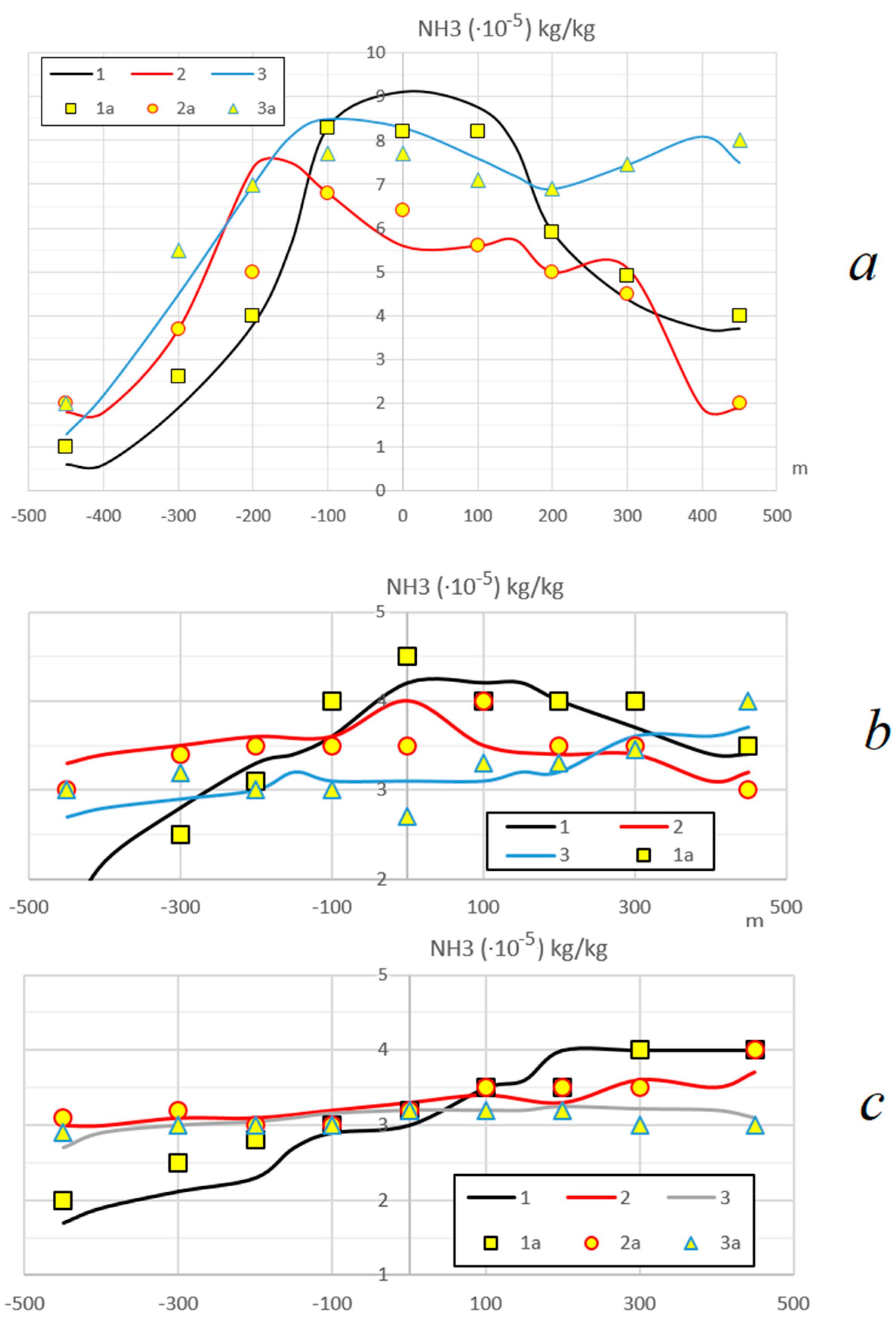
Figure 11 shows a comparison of the theoretical profile of the mass concentration of ammonia and the experimentally obtained values. In analyzing the presented diagrams, it can be noted that, in general, despite some discrepancies, the shape of the profiles and the concentration values are close and the discrepancy does not exceed 15%. Similarly to the velocity profiles, it is noted that the obtained profiles have a smaller spread of values, in comparison with the profiles obtained using calculations. This can also be explained by averaging the readings on the device over the measurement interval.
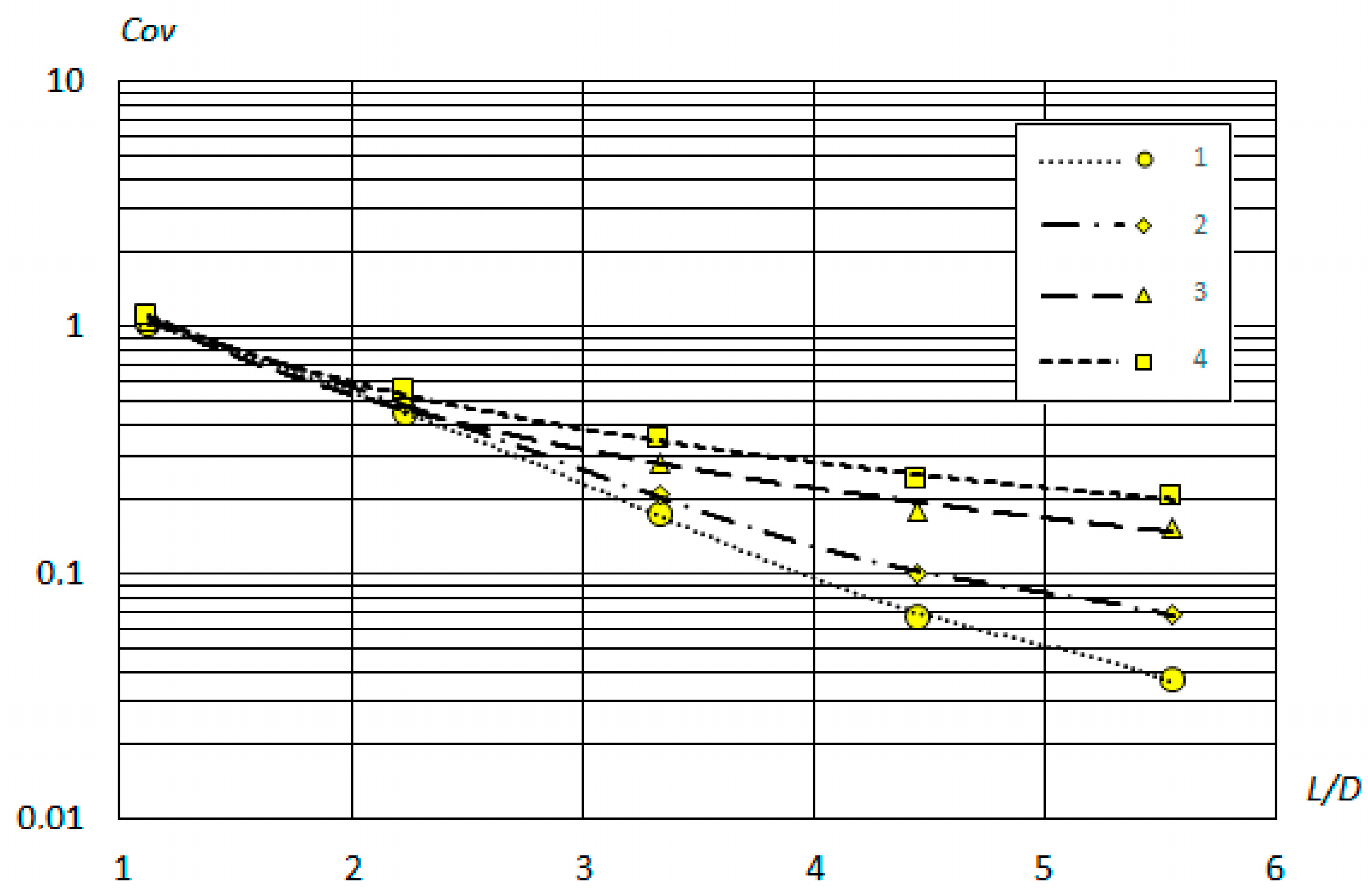
A calculation of the
Cov parameter (taking into account the relative deviation of concentrations from the average value in each section and at different Re numbers) was carried out using (1) to quantitatively assess the uniformity of the ammonia distribution. The dependence of the
Cov value on the L/D ratio at different Re values for flue gasses is shown in
Figure 12.
5. Discussions
The obtained dependencies show that the degree of homogeneity increases from the point of ammonia supply along the mixer length. This is reflected in the achievement of Cov = 0.037–0.2 at different Re values.
Up to the central part of the mixing section (about 2.5 L/D from the ammonia feed point), the flow homogeneity has similar values for all flue gas flow rate variants and reaches
Cov = 0.2–0.3. It is probable that the influence of the formed turbulent jets manifests itself above this interval. In the section above 2.5 L/D, the mixing quality varies significantly. This can be explained by the large contribution of turbulent diffusion in the flow. At L/D > 4.5, the growth of
Cov slows down due to the reduced influence of turbulent jets formed in the mixer on diffusion (probably).
Cov reaches 0.037 at the maximum load at L/D = 5.55 (corresponding to mixer length L = 5 m). The minimum ratio corresponding to
Cov = 0.05 is L/D = 5. At a load of 85% of the maximum (Re = 222,000), according to the graph in
Figure 11, it is assumed that the required mixing quality will be achieved at L/D = 5.5. At lower loads, a significant length of the mixing zone may be required. A decrease in
Cov with a decrease in flue gas flow imposes restrictions on the use of the mixer, since this may affect the final quality of the DeNOx unit. Calculations have shown that in this case, it will be necessary to use a different mixer size, which will allow for maintaining a similar hydrodynamic situation (Re = 220,000–260,000)
The results of comparing the distribution of velocities and concentrations obtained by simulation and experiment should be discussed separately. The general method for determining experimental values at nodal points has been described earlier. It should be noted that the values were averaged during data processing, since they changed over time, which is associated with the continuous process of swirling flows in the mixer. The average scatter of values when measuring at a distance of 2.5 m did not exceed 15%; at a distance of 4 m, no more than 10%; and at a distance of 5 m, it decreased to 8%. At the same time, with an increase in the flue gas flow rate, the scatter of the measured values also decreases somewhat.
In analyzing the data presented in
Figure 8 and
Figure 11, it can be noted that the nature of the change in velocity and concentration during simulation generally corresponds to the measured values of these parameters. The discrepancy between the experimental and theoretical values in the velocity diagrams (
Figure 8) and concentration diagrams (
Figure 11) decreases with an increase in the velocity of the flue gasses and an increase in the distance. The discrepancy can reach 20% at a distance of 2.5 m from the ammonia injection point. Later, it does not exceed 5–10%. This can be explained by complex transient processes in the mixer, the occurrence of flow breaks, the imperfection of the selected grid during modeling, and the measurement error with the selected method.
However, all this has an insignificant effect on the final result achieving the required homogeneity in the final section and sufficient accuracy of the obtained modeling results in this section (4–5 m from the ammonia injection point). It can be concluded that the model is verified with the output concentration values. Thus, the working range of the mixer should not be reduced by more than 20% of the maximum load value given. Reducing the flue gas load leads to an increase in the mixing area and a decrease in the degree of homogeneity. A decrease in the homogeneity of the mixture leads to a breakthrough of NOx gasses to subsequent stages of the unit operation. Since the DeNOx unit is part of the unit for absorbing CO
2 from flue gasses, an increase in the NOx concentration affects the rate of degradation of the absorbent (MEA) [
20]. In addition, increased NOx content has a negative impact on the environment. This can be compensated for by increasing the mixing area, increasing the initial concentration of the reagent, and reducing the mixer diameter. In addition, it is possible to supply excess reagent when using one mixer size to compensate for an uneven distribution. In this case, the minimum reagent concentration is achieved at each point of the mixer. This method is used in production, and the supply of ammonia is adjusted according to sensor readings.
Table 2 shows comparative results of the efficiency of mixer designs presented in the scientific literature.
In comparing the obtained results with similar ones presented in [
9], it can be noted that the mixer under study works better than most of those presented in [
9], comparable to the SMX and SMV paddle mixers, which, in different modifications, have effective mixing in sections L/D = 6.7 (SMX) and L/D less than 6.2 m (SMV). However, these mixers are more complex in design and have the highest hydraulic resistance of those presented in [
9]. In analyzing the data presented in [
11], it is noted that the mixer under study is superior to or comparable to those presented in [
11]. It has a shorter mixing section length L/D and is significantly inferior only to the Sulzer Compact X mixer (L/D = 3.2). It should be noted that the studies involved mixers with a smaller diameter (2″–6″), which does not take into account the scale effect in the comparison. Work [
12] also considered a mixer with a similar design, but with a larger number of blades, and therefore a more complex design. At the same time, the mixer studied in this work is somewhat inferior to the one presented in [
12]. It can be concluded that the developed mixer corresponds to modern developments in terms of mixing quality but is simpler in design and more compact.
6. Conclusions
The following conclusions can be drawn from the results of the work performed:
1. As a result of modeling the developed mixer, acceptable mixing quality was noted. Cov = 0.05 was achieved in the L/D = 5 section at a maximum gas load of 35,000 kg/h.
2. When analyzing the velocity distribution, it was found that when the mixer is operating, velocity layers are formed in the center, and individual streams are formed along the periphery of the mixer. The comparison of the calculated velocities with those experimentally obtained in the control section confirms the overall model of the flow distribution. Also, the comparison carried out using the concentrations in the control section confirms the adequacy of the selected model.
3. When the flow rate decreases by more than 20% of the specified value, the flow non-uniformity increases and reaches values of Cov = 0.2 at 50% supply of flue gasses and reagent to the mixer. This can affect the neutralization of NOx gasses. Calculations show that it will be necessary to use a mixer of a smaller diameter, in which the required hydrodynamic conditions Re = 220,000–260,000 will be maintained to eliminate this effect.
4. In comparing the performance of the mixer under study with the literature data, it was found that it is generally comparable to those used in industry in terms of mixing quality and is only slightly inferior to some designs. At the same time, the device under consideration has a simpler design, is compact, and is easy to maintain.
As a result of the conducted research, it can be concluded that the developed mixer generally corresponds to the modern level of technology, but the mixing quality can also be improved with further modernization. Further directions of research can be studying the influence of the ammonia injection point into the mixer, the mutual direction of the mixed flows, the number and shape of the swirler blades, and their angle on the mixing quality. All this can lead to an improvement in the quality of the distribution even at low flue gas flow rates and reduction in the mixing length. At the same time, the total energy costs of the mixing process can increase. Identifying optimal parameters and searching for designs with a different set of performance characteristics is another urgent task for research.


 and
and 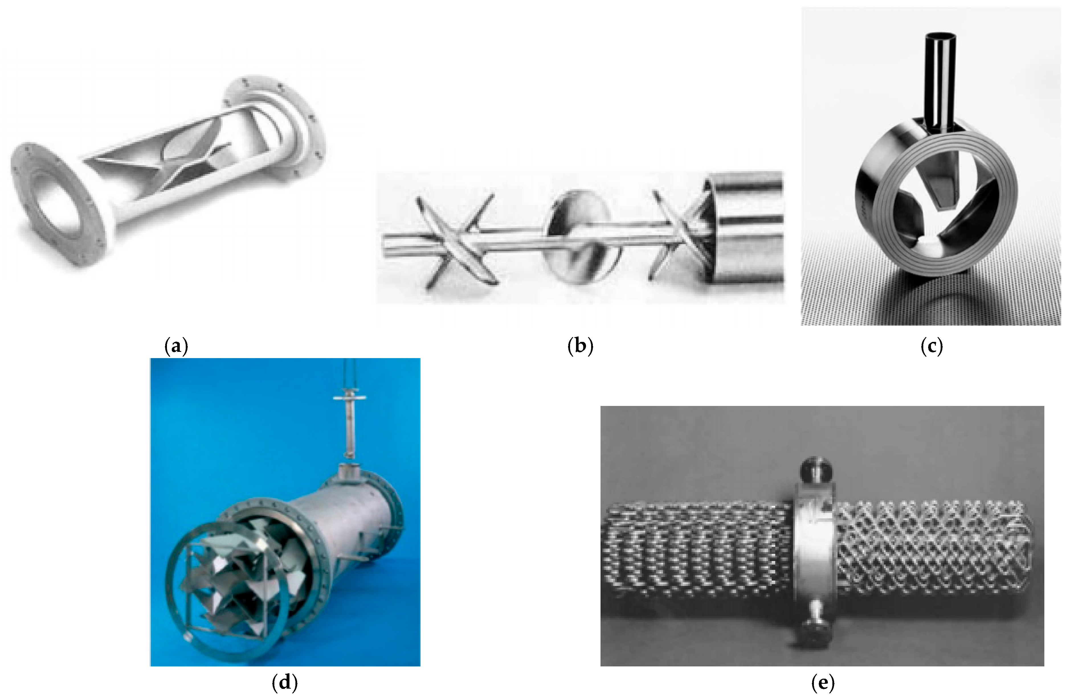


