Optimizing Rural MG’s Performance: A Scenario-Based Approach Using an Improved Multi-Objective Crow Search Algorithm Considering Uncertainty

Abstract

In recent years, the growth of utilizing rural microgrids (RMGs) has been accompanied by various challenges. These necessitate the development of appropriate models for optimal generation in RMGs and RMGs’ coordination. In this paper, two distinct models for RMGs are presented. The first model includes an islanded rural microgrid (IRMG) and the second model consists of three RMGs that are interconnected with one another and linked to the distribution network. The proposed models take into account the uncertainty in load, photovoltaics (PVs), and wind turbines (WTs) with consideration of their correlation by using a scenario-based technique. Three objective functions are defined for optimization: minimizing operational costs including maintenance and fuel expenses, reducing voltage deviation to maintain power quality, and decreasing pollution emissions from fuel cells and microturbines. A new optimization method, namely the Improved Multi-Objective Crow Search Algorithm (IMOCSA), is proposed to solve the problem models. IMOCSA enhances the standard Crow Search Algorithm through three key improvements: an adaptive chaotic awareness probability to better balance exploration and exploitation, a mutation mechanism applied to the solution repository to prevent premature convergence, and a K-means clustering method to control repository size and increase algorithmic efficiency. Since the proposed problem is a multi-objective non-linear optimization problem with conflicting objectives, the idea of the Pareto front is used to find a group of optimal solutions. To assess the effectiveness and efficiency of the proposed models, they are implemented in two different case studies and the analysis and results are illustrated.

1. Introduction

An RMG is a part of the distribution network which encompasses DGs, energy storage devices, and various loads. DGs include various technologies such as MTs, FCs, PVs, WTs, etc. Since some of these DGs are used to supply RMGs’ requirements, making coordination between these sources and determining their production levels highly important. Furthermore, when RMGs are interconnected with each other, the issue of coordination and cooperation by considering objectives such as cost and pollution emission through DGs in RMGs becomes significant. The utilization of DGs in MGs minimizes transmitted power in transmission lines, delays generation and transmission infrastructure expansion, decreases fossil fuel consumption, and improves power system efficiency [1]. Despite the mentioned benefits, MGs also pose challenges. Since each MG consists of various types of DGs, coordinating their operations and creating a suitable method for optimal MG generation are essential [2]. Two modes of operation are available for MGs: connected to grid mode and islanded mode. An “islanded MG” only operates independently of the main grid and cannot be connected to a broader power system. MGs have their own specific electricity sources which are complemented by an energy storage system. MGs are often used in locations where transmitting and distributing electricity from a centralized energy source to operate take place over a long distance and are costly [3]. Collaboration among various DGs in an islanded MG enhances energy consumption efficiency and minimizes the operational costs of MGs. Numerous studies have been conducted in this field and some of them are discussed below. An energy management framework, which merges active and reactive methods to effectively tackle uncertainties associated with generation and demand, was proposed in [4] during the operation of MGs in both islanded and interconnected modes. In [5], in order to optimize utilization of DGs within each MG and transmit the supported power to the distribution network or MGs with power shortages, methods such as the implementation of a robust EMS and appropriate power distribution in SGs have been proposed. Under normal conditions, power dispatching was carried out in a highly balanced manner which took into account both cost considerations and eco-management [6]. Strategies for energy management and utilization of RMGs have been utilized [7,8]. In [9,10], the decentralized and centralized energy management systems of multiple MGs were studied and analyzed. In [11], an approach involving double-layer coordination for energy management was proposed for MGs’ operation. A robust energy management method for MGs with uncertainties was introduced in [12]. In [13], a distributed energy management method based on data related to the exchange of energy among neighboring MGs was presented. Additionally, an optimal and coordinated energy management system for MGs along with a new index for modeling uncertainty was presented in [14]. In this paper, according to the increasing penetration of DGs and the growing demand for electricity in RMGs, two models for RMGs are proposed to solve the problems by optimizing cost, voltage deviation, and pollution emission. These problems include optimal scheduling of distributed generation in IRMGs, modeling uncertainty related to RESs and load, coordinated operation of RMG clusters, and coordination between RMGs and the distribution network.

Recent advancements in artificial intelligence have expanded the scope of optimization methods, with neural networks and machine learning approaches increasingly being adopted for microgrid optimization. DNNs have shown significant promise in addressing the limitations of traditional optimization methods, particularly in handling system uncertainties and complex operational constraints. For example, DNN-based approaches have been demonstrated to significantly reduce the solution time for intra-day rolling optimization to milliseconds while maintaining solution quality [15]. Hybrid approaches combining CNNs with Bi-LSTM networks have also been effectively employed for rapid decision making in microgrid scheduling, offering improved computational efficiency and decision-making accuracy compared to conventional methods [15].

Another notable development is the use of model-free reinforcement learning techniques for multi-microgrid energy management [16]. These approaches have demonstrated high accuracy in estimating power exchange, with studies reporting average relative errors as low as 0.96 for 2400 test samples [16]. Additionally, deep learning methods have proven valuable in maintaining user privacy while optimizing system performance, as they can effectively simulate microgrid operations without requiring access to local generation or consumption data [16].

In the domain of standalone hybrid microgrids, EMM incorporating ANNs has achieved significant improvements, including reductions in prediction errors by 59% for single-step and 56% for multiple-step energy parameter estimations [17]. However, neural network-based approaches also face certain limitations, such as challenges in predicting parameters like the SoC of energy storage systems and potential issues with input variable selection [17]. Moreover, these methods can be influenced by network topology and various uncertainties, including load variations and fluctuations in distributed renewable generation [16].

Since the abovementioned problems are non-linear, metaheuristic techniques are utilized. Many studies have been carried out focusing on the utilization of metaheuristic algorithms to optimize the operation of MGs. Some used algorithms include PSO [18], GA [19], DE [20], TLBO [21], and WOA [22]. In this paper, CSA [23] is utilized. However, to address limitations in existing CSA variants and enhance its performance for multi-objective optimization, this paper proposes IMOCSA. IMOCSA incorporates two key enhancements: (1) an adaptive chaotic AP to better balance exploration and exploitation throughout the optimization process and (2) a mutation mechanism applied to the solution repository to prevent premature convergence. Additionally, the K-means method is employed to control the size of the repository and increase algorithmic efficiency. These modifications aim to address challenges such as inconsistent awareness probabilities, limited exploration in later iterations, and insufficient diversity in Pareto front representation, ensuring more robust and efficient optimization performance. Therefore, the key contributions of this paper are as follows:

• The paper presents two renewable energy source-based RMG models: IRMG and a system of three interconnected RMGs linked to the distribution network.
• It proposes a new sophisticated scenario-based methodology incorporating correlations among load, PV, and WT uncertainties, enhancing RMG modeling fidelity.
• IMOCSA is introduced, featuring a chaotic-based initial population generation, an adaptive chaotic AP, a roulette-wheel-based position-updating method, and a new mutation strategy, enhancing multi-objective optimization efficacy for RMGs.

In the following, in Section 2, the objective functions and constraints related to both models are presented. In Section 3, modeling of input random variables and scenario selections are discussed. In Section 4, IMOCSA is introduced for optimizing the models. In Section 5, simulation results are presented and are analyzed. In Section 6, the findings of the study are concluded.

2. Problem Formulation

Before presenting the mathematical models, it is essential to understand the key DG technologies utilized in the RMG systems and their operational characteristics:

MTs are compact combustion turbines with generation capacities typically ranging from 25 to 500 kW. MTs operate on the Brayton cycle where compressed air is mixed with fuel, burned in a combustion chamber, and the resulting hot gas drives a turbine connected to a generator. They offer high operational efficiency, reaching up to 80% in combined heat and power applications. MTs feature fast startup and shutdown capabilities, along with the ability to use various fuel types, including natural gas, biogas, and diesel. Their design incorporates fewer moving parts, resulting in low maintenance requirements. The stable power output makes them particularly suitable for baseload operation in microgrid systems.

FCs are electrochemical devices that convert chemical energy directly into electrical energy through reactions between hydrogen and oxygen. In the process, hydrogen fuel is split into protons and electrons at the anode, with protons passing through a membrane while electrons travel through an external circuit. Oxygen then combines with protons and electrons at the cathode to produce water. FCs achieve high electrical efficiency of 40–60% and produce near-zero emissions when using hydrogen fuel. Their operation is notably quiet due to the absence of moving parts, and they provide reliable continuous power generation. The modular design allows for flexible capacity scaling to meet varying power requirements.

PVs convert sunlight directly into electricity using semiconductor materials exhibiting the photovoltaic effect. The system architecture includes PV modules for power generation, inverters for DC to AC conversion, maximum power point tracking (MPPT) systems for optimization, and supporting structures and wiring. PV systems produce zero operational emissions and feature high reliability due to the absence of moving parts. Their power output varies with solar irradiance and temperature, requiring significant installation area and limiting generation to daylight hours.

WTs harness wind energy through aerodynamic blades that capture kinetic energy from wind, utilizing a gearbox to increase rotational speed in most designs, and a generator to convert mechanical energy to electrical power. The power output varies cubically with wind speed, with typical cut-in wind speeds of 3–5 m/s and rated power achieved at 10–15 m/s. For safety, turbines implement cut-out mechanisms at high wind speeds. Like PV systems, WTs produce zero operational emissions during power generation.

2.1. The First Model (IRMG)

The operation of islanded MGs emphasizes power sharing and system stability [24]. The proposed model for the IRMG is developed based on assumptions regarding the load curve of power consumption and IL for residential users. Three objective functions are defined for the model. The first is the operational cost ($f_1$), which minimizes the total cost of operating the IRMG, accounting for power generation, maintenance costs, and IL compensation (1). The second is voltage deviation ($f_2$), which minimizes the deviation of bus voltages from a reference level, ensuring voltage stability and system reliability (2). The third is pollution emissions ($f_3$), which minimizes the environmental impact by reducing emissions from power generation units such as MTs and FCs (3).

$$\min f_1\left(X_1\right)={\displaystyle \sum _{t=0}^{T=24}\left[\begin{array}{l}{\rho }_{PV}{P}_{PV}^t+{\rho }_{WT}{P}_{WT}^t+{\rho }_{BAT}\left(P_{BATPV}^t+P_{BATWT}^t\right)\\ +{\rho }_{FC}{P}_{FC}^t+{\rho }_{MT}{P}_{MT}^t+{\rho }_{IL}{P}_{IL}^t\end{array}\right]}$$

(1)

$$\min f_2\left(X\right)={\displaystyle \frac{{\displaystyle \sum _{t=1}^{T=24}{\displaystyle \sum _{i=1}^{N_{bus}}\left(\frac{\left|V_{ref}-V_i^t\right|}{V_{ref}}\right)}}}{N_{bus}}}$$

(2)

$$\min f_3\left(X\right)={\displaystyle \sum _{t=1}^{T=24}\left(P_{FC}^t{E}_{FC}+P_{MT}^t{E}_{MT}\right)}$$

(3)

$$X=\left[P_{WT}{P}_{PV}{P}_{FC}{P}_{MT}{P}_{BATPV}{P}_{BATWT}\right]$$

(4)

$$P_{WT}={\left[P_{WT}^1{P}_{WT}^2\cdots P_{WT}^T\right]}_{1\times T}$$

(5)

$$P_{PV}={\left[P_{PV}^1{P}_{PV}^2\cdots P_{PV}^T\right]}_{1\times T}$$

(6)

$$P_{FC}={\left[P_{FC}^1{P}_{FC}^2\cdots P_{FC}^T\right]}_{1\times T}$$

(7)

$$P_{MT}={\left[P_{MT}^1{P}_{MT}^2\cdots P_{MT}^T\right]}_{1\times T}$$

(8)

$$P_{BATPV}={\left[P_{BATPV}^1{P}_{BATPV}^2\cdots P_{BATPV}^T\right]}_{1\times T}$$

(9)

$$P_{BATWT}={\left[P_{BATWT}^1{P}_{BATWT}^2\cdots P_{BATWT}^T\right]}_{1\times T}$$

(10)

In addition to DG units, the model incorporates a BAT associated with WT and PV units. The relationship between BAT capacity and its charge/discharge power over time is governed by (11) that reflects the energy dynamics of the BAT, considering self-discharge rates, charging/discharging efficiencies, and power constraints.

$$E_{BAT}^t=E_{BAT}^{t-1}\left(1-\sigma \right)+\Delta T\times U_{ch}^t\times P_{ch}\times {\eta }_{ch}-\Delta T\times U_{dis}^t\times {\displaystyle \frac{P_{dis}}{{\eta }_{ch}}}$$

(11)

The model also includes a set of constraints to ensure practical and feasible operation. The power balance constraint (12) ensures that the total power generated matches the total load demand (including IL) at every time step, maintaining energy balance. Generation limits (13)–(16) define the permissible operational ranges for each DG unit (e.g., PV, WT, MT, FC). These constraints prevent overloading and ensure that generation stays within technical and physical limits. Renewable energy curtailment constraints include the maximum wind rejection (17), which limits the amount of wind energy that can be curtailed, and the maximum discarded solar energy (18), which restricts the extent to which solar energy can be wasted, ensuring optimal utilization of renewable resources.

$${\displaystyle \sum _{t=1}^T{P}_{Load}^t}={\displaystyle \sum _{t=1}^T\left[\begin{array}{l}{P}_{WT}^t+P_{BATWT}^t+P_{PV}^t+P_{BATPV}^t\\ +P_{MT}^t+P_{FC}^t+P_{IL}^t\end{array}\right]},P_{IL}^t\ge 0$$

(12)

$$P_{MT,\min }^t\le P_{MT}^t\le P_{MT,\max }^t$$

(13)

$$P_{FC,\min }^t\le P_{FC}^t\le P_{FC,\max }^t$$

(14)

$$P_{WT,\min }^t\le P_{WT}^t\le P_{WT,\max }^t$$

(15)

$$P_{PV,\min }^t\le P_{PV}^t\le P_{PV,\max }^t$$

(16)

$$P_{WT}^t\ge \left(1-{\alpha }_w\right)P_{WT,\max }^t$$

(17)

$$P_{PV}^t\ge \left(1-{\beta }_s\right)P_{PV,\max }^t$$

(18)

Battery energy constraints (19)–(23) ensure the BAT’s energy levels remain within defined bounds, maintaining operational integrity. These include capacity limits (19) and (20), which keep the BAT’s energy levels within acceptable bounds, and charging/discharging power limits (21) and (22), which specify the maximum permissible rates of charging and discharging for the BAT. The state of charge equality constraint (23) mandates that the BAT returns to its initial state of charge by the end of the operational cycle, ensuring readiness for subsequent periods. Voltage constraints (24) ensure that the bus voltages across the IRMG remain within acceptable limits, preventing operational instability and equipment damage.

$${\underset{\_}{E}}_{BAT}\le E_{BAT}\le {\overline{E}}_{BAT}$$

(19)

$$E_{BAT}^{t=0}=E_{BATINT}$$

(20)

$${\underset{\_}{P}}_{ch}\le P_{ch}\le {\overline{P}}_{ch}$$

(21)

$${\underset{\_}{P}}_{dis}\le P_{dis}\le {\overline{P}}_{dis}$$

(22)

$$U_{ch}+U_{dis}\le 1$$

(23)

$$V_{\min }\le \left|V_i^t\right|\le V_{\max }$$

(24)

The combination of these objectives and constraints provides a robust framework for optimizing the IRMG’s performance while maintaining stability, reliability, and environmental sustainability.

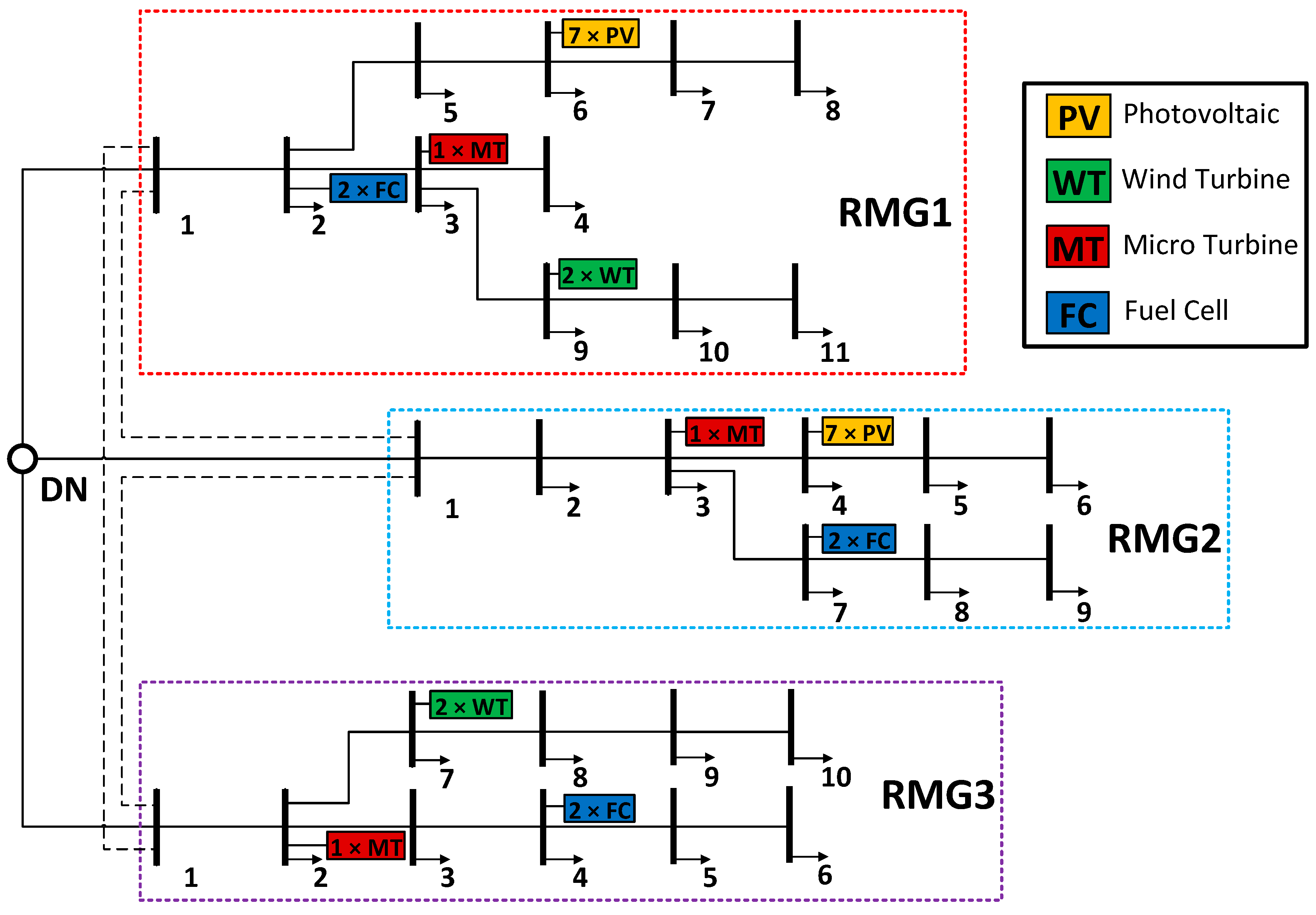
2.2. The Second Model (Three RMGs and Distribution Network)

In this paper, rather than only considering the cost objective function ($f_1$) as established based on cooperative game theory in [25], two additional objective functions are introduced: voltage deviation ($f_2$) and pollution emission ($f_3$) (25)–(27). These objective functions collectively aim to optimize the performance of three interconnected RMGs linked to a distribution network. The inclusion of voltage deviation and pollution emission objectives highlights the importance of ensuring power quality and minimizing environmental impact alongside economic considerations.

$$\min f_1\left(X\right)={\displaystyle \sum _{n=1}^N{\displaystyle \sum _{t=1}^T\left[\begin{array}{l}{\rho }_{WT}{P}_{WT,n}^t+{\rho }_{PV}{P}_{PV,n}^t+\\ {\rho }_{FC}{P}_{FC,n}^t+{\rho }_{MT}{P}_{MT,n}^t+\\ \left(1-\gamma \right){\lambda }_{bgrid}{P}_{bgrid}^t+\gamma {\lambda }_{sgrid}{P}_{sgrid}^t\end{array}\right]}}$$

(25)

$$\min f_2\left(X\right)={\displaystyle \sum _{n=1}^N\left[\frac{{\displaystyle \sum _{t=1}^T{\displaystyle \sum _{i=a}^{N_{bus,n}}\left(\frac{\left|V_{ref}-V_{i,n}^t\right|}{V_{ref}}\right)}}}{N_{bus,n}}\right]}$$

(26)

$$\min f_3\left(X\right)={\displaystyle \sum _{n=1}^N{\displaystyle \sum _{t=1}^T\left[\begin{array}{l}(1-\gamma )P_{bgrid}^t{E}_{gird}+\\ P_{MT,n}^t{E}_{MT}+P_{FC,n}^t{E}_{FC}\end{array}\right]}}$$

(27)

$$X={\left[P_{WT}{P}_{PV}{P}_{FC,}{P}_{MT}\right]}_{1\times T\times N\times n}$$

(28)

$$P_{WT}={\left[P_{WT,1}^1{P}_{WT,1}^2\cdots P_{WT,1}^T{P}_{WT,2}^1{P}_{WT,2}^2\cdots P_{WT,2}^T\cdots P_{WT,N}^T\right]}_{1\times T\times N}$$

(29)

$$P_{PV}={\left[P_{PV,1}^1{P}_{PV,1}^2\cdots P_{PV,1}^T{P}_{PV,2}^1{P}_{PV,2}^2\cdots P_{PV,2}^T\cdots P_{PV,N}^T\right]}_{1\times T\times N}$$

(30)

$$P_{MT}={\left[P_{MT,1}^1{P}_{MT,1}^2\cdots P_{MT,1}^T{P}_{MT,2}^1{P}_{MT,2}^2\cdots P_{MT,2}^T\cdots P_{MT,N}^T\right]}_{1\times T\times N}$$

(31)

$$P_{FC}={\left[P_{FC,1}^1{P}_{FC,1}^2\cdots P_{FC,1}^T{P}_{FC,2}^1{P}_{FC,2}^2\cdots P_{FC,2}^T\cdots P_{FC,N}^T\right]}_{1\times T\times N}$$

(32)

The model introduces a switch ($\gamma$) to represent the state of electricity purchasing and selling. When $\gamma$ equals 1, the RMG coalition operates in surplus power mode and sells electricity to the distribution network. Conversely, when $\gamma$ equals 0, the coalition experiences a power shortage and purchases electricity from the distribution network. This mechanism enables dynamic interaction between the RMGs and the distribution network, ensuring adaptability to varying power supply and demand conditions.

Unlike the first model, the second model does not include constraints related to BAT or forced shutdown scenarios. The power balance constraint, which ensures that the total power generated and exchanged matches the total load demand at each time step, is expressed as a core equation of this model.

$${\displaystyle \sum _{n=1}^N{\displaystyle \sum _{t=1}^T{P}_{Load,n}^t}}={\displaystyle \sum _{n=1}^N{\displaystyle \sum _{t=1}^T\left(\begin{array}{l}{P}_{WT,n}^T+P_{PV,n}^T+\\ P_{FC,n}^T+P_{PV,n}^T\end{array}\right)}}+{\displaystyle \sum _{t=1}^T\left(P_{bgrid}^t-P_{sgrid}^t\right)}$$

(33)

The remaining constraints, such as generation limits, renewable energy curtailment, and voltage stability, are consistent with those defined in the first model. These constraints collectively ensure that the operational boundaries of the RMGs and their interaction with the distribution network adhere to technical, economic, and environmental standards. This model expands the scope of optimization by incorporating the interconnected operation of multiple RMGs and their coordinated interaction with the larger power distribution network, providing a holistic approach to rural microgrid management.

3. Scenario Generation and Mitigation

Various approaches, including the scenario-based method [26], PEM [27], MC method [28], and UT [29], have been utilized to address uncertainty in load forecasting and RESs’ output. This paper utilizes a scenario-based method to model stochastic parameters of wind speed, solar irradiance, and load. Initially, a large number of scenarios are generated using an MC and then reduced to a specific number.

3.1. Modeling of Load, Wind Speed, and Solar Irradiance

The uncertainty of the load, wind speed, and solar irradiance are modeled using a normal distribution [30], Weibull distribution [31] and beta distribution [32], respectively.

3.2. Proposed Scenario Generation and Reduction

More scenarios improve accuracy but increase the calculation volume, leading to time-consuming simulations [33]. A wide range of scenarios for input variables are initially generated, after which a scenario reduction strategy is implemented to reach a pre-defined number [30]. The proposed approach considers the correlation between random variables, which was not previously considered. The steps of scenario generation and reduction are described below:

• First, for each random variable, a set of independent random numbers following a standard normal distribution is generated, corresponding to the number of scenarios.

  $$R=normrnd\left(0,1,[scenarios,Numberofvariables]\right)$$

  (34)
• The matrix $R$ is multiplied by the Cholesky matrix.

  $$X=chol\left(C\right)\times R$$

  (35)
• CDF is calculated from the standard normal distribution $X$.

  $$\phi =CD{F}_{Noraml}\left(X\right)$$

  (36)
• Then, scenarios are generated using $CD{F}^{-1}$ for each variable based on the defined distribution functions while preserving their correlation.

  $$Y=CD{F}_{\left(\mathrm{Distribution}\mathrm{function}\mathrm{type}\right)}^{-1}\left(\phi \right)$$

  (37)
• Finally, the generated scenarios are reduced to the desired number and WT and PV output power are calculated [30].

4. Proposed Crow Search Algorithm

4.1. CSA

CSA [23] is a metaheuristic technique that offers optimal mathematical methods. To run CSA, the following steps need to be considered:

Step 1:

Define the decision variables and CSA parameters.

Step 2:

Randomly place $N_c$ in a d-dimensional search space as the initial population. Each crow is a potential solution.

$$Crows=\left[\begin{array}{cccc}{X}_1^1& X_2^1& \cdots & X_d^1\\ X_1^1& X_2^1& \cdots & X_d^1\\ ⋮& ⋮& \ddots & ⋮\\ X_1^{N_c}& X_2^{N_c}& \cdots & X_d^{N_c}\end{array}\right]$$

(38)

Step 3:

Initialize each crow’s memory, assuming they have hidden food at their initial positions because of lack of experience.

$$Memory=\left[\begin{array}{llll}{M}_1^1& M_2^1& \cdots & M_d^1\\ M_1^1& M_2^1& \cdots & M_d^1\\ ⋮& ⋮& \ddots & ⋮\\ M_1^{N_c}& M_2^{N_c}& \cdots & M_d^{N_c}\end{array}\right]$$

(39)

Step 4:

Calculate the objective function value for each crow.

Step 5:

In each iteration, a crow $i$ updates its position by randomly selecting another crow $j$ to chase for food $M^{j,iter}$. Depending on ${AP}^{j,iter}$, crow $i$ either approaches $M^{j,iter}$ or is deceived.

$$X^{i,iter+1}=\left\{\begin{array}{l}{X}^{i,iter}+rand\times fl\times (M^{j,iter}-X^{i,iter})rand\ge A{P}^{j,iter}\\ arandompositionotherwise\end{array}\right.$$

(40)

Step 6:

By meeting the constraints, the new position of the crow is accepted and the objective function value is calculated.

Step 7:

If the new position has a better objective function value, update the crow’s memory with the new position.

$$M^{i,iter+1}=\left\{\begin{array}{l}{X}^{i,iter+1}f\left(X^{i,iter+1}\right)isbetterthanf\left(M^{i.iter}\right)\\ M^{i,iter+1}otherwise\end{array}\right.$$

(41)

Step 8:

Repeat steps 5–8 until the number of iterations reaches ${iter}_{max}$. The best memory position is reported as the optimal solution when the termination criterion is met.

4.2. IMOCSA

In this paper, several methods are employed to enhance the overall performance of CSA. Initially, in IMOCSA, the initial population is generated through the tent method, according to (42)–(45). This approach potentially leads to faster convergence and reduced sensitivity to outliers, so an appropriate balance between exploration and exploitation is struck. Furthermore, it offers improved stability across multiple runs and can be adapted to match the expected structure of the problem space.

$$X^{i,Initial}=X_{\min }+R_{tent,m}^{i,Initial}\times \left(X_{\max }-X_{\min }\right)$$

(42)

$$R_{tent,m}^{1,Initial}=rand\left(1,d\right)$$

(43)

$$R_{tent,m}^{1,Initial}\notin \left\{0,0.25,0.5,0.75,1\right\}\forall m=1,2,\dots ,d$$

(44)

$$R_{tent,m}^{i+1,Initial}=\left\{\begin{array}{cc}2\cdot R_{tent,m}^{i,Initial}& R_{tent,m}^{i,Initial}<0.5\\ 2\cdot \left(1-R_{tent,m}^{i,Initial}\right)& otherwise\end{array}\right.$$

(45)

Secondly, the balance between diversification and intensification, which is regulated by AP, significantly affects the performance of CSA [34]. It is noted that intensification is promoted by smaller AP values, while larger values enhance diversification. The initiative proposed in [35] enhances CSA by using an adaptive chaotic $AP$ for single-objective problems. This paper extends this approach to multi-objective problems by introducing ${\omega }_n$, thus redefining $AP$ for such problems.

$$A{P}^{j,iter}=Z^{iter}\times \left({\displaystyle \frac{{\displaystyle \sum _{n=1}^{N_{obj}}{\omega }_n\left(\frac{f_{memory,n}^{j,iter}-f_{\min ,n}}{f_{\max ,n}-f_{\min ,n}}\right)}}{f_{\max ,memory}^{iter}}}\right)\times {\alpha }_{AP}$$

(46)

${\alpha }_{AP}$ and $Z^{iter}$ are the constant coefficient $\mathrm{a}\mathrm{n}\mathrm{d}$ chaotic sequence, respectively [35].

$$f_{\max ,memory}^{iter}=\max \left({\left[\begin{array}{l}{\displaystyle \sum _{n=1}^{N_{obj}}{\omega }_n\left(\frac{f_{memory,n}^{1,iter}-f_{\min ,n}}{f_{\max ,n}-f_{\min ,n}}\right)}\\ {\displaystyle \sum _{n=1}^{N_{obj}}{\omega }_n\left(\frac{f_{memory,n}^{2,iter}-f_{\min ,n}}{f_{\max ,n}-f_{\min ,n}}\right)}\\ ⋮\\ {\displaystyle \sum _{n=1}^{N_{obj}}{\omega }_n\left(\frac{f_{memory,n}^{N_c,iter}-f_{\min ,n}}{f_{\max ,n}-f_{\min ,n}}\right)}\end{array}\right]}_{N_c\times 1}\right)$$

(47)

IMOCSA employs an adaptive strategy for position updating when the awareness probability of the jth crow falls below a random number, according to (48). This approach utilizes three distinct methods, selected via a roulette wheel mechanism. Initially, for the first 25 iterations, each method has an equal probability of selection, with the selection probability vector set to [1,1,1]. After the 25th iteration, the algorithm introduces a performance-based adaptation. If a method obtains a superior solution compared to the others, its selection probability is incrementally increased by one unit. This dynamic adjustment allows the algorithm to favor more effective methods over time, potentially enhancing its exploration and exploitation capabilities. The first method [36] improves local search ability, the second method [37] enhances convergence speed, and the third method reduces the likelihood of getting stuck in local optima. This combination of methods aims to balance the algorithm’s search efficiency and solution quality throughout the optimization process.

$$X^{i,iter+1}=\left\{\begin{array}{r}{X}^{i,iter}+rand\times fl\times \left(M^{j,iter}-X^{i,iter}\right)rand\ge A{P}^{j,iter}\\ X^{i,iter}+rand\times \left(x_{gbest}-TF\cdot x_{population}^{mean}\right)method=1\\ x_{gbest}+{\displaystyle \frac{5\times rand}{1000}}\times \left(X_{\max }-X_{\min }\right)method=2\\ X_{\min }+rand\times \left(X_{\max }-X_{\min }\right)method=3\end{array}\right.$$

(48)

To prevent getting stuck in local optima, a mutation on the solution repository is proposed. The mutation is applied by randomly selecting two members, $R_1$ and $R_2$, from the solution repository ($R_1$ ≠ $R_2$). AP for the desired mutation is calculated as follows:

$$A{P}_{mutation}^{R_2,iter}=Z^{iter}\times \left({\displaystyle \frac{{\displaystyle \sum _{n=1}^{N_{obj}}{\omega }_n\left(\frac{f_{rep,n}^{R_2,iter}-f_{\min ,n}}{f_{\max ,n}-f_{\min ,n}}\right)}}{f_{\max ,rep}^{iter}}}\right)\times {\alpha }_{AP}$$

(49)

$$f_{\max ,rep}^{iter}=\max \left({\left[\begin{array}{c}{\displaystyle \sum _{n=1}^{N_{obj}}{\omega }_n\left(\frac{f_{rep,n}^{1,iter}-f_{\min ,n}}{f_{\max ,n}-f_{\min ,n}}\right)}\\ {\displaystyle \sum _{n=1}^{N_{obj}}{\omega }_n\left(\frac{f_{rep,n}^{2,iter}-f_{\min ,n}}{f_{\max ,n}-f_{\min ,n}}\right)}\\ ⋮\\ {\displaystyle \sum _{n=1}^{N_{obj}}{\omega }_n\left(\frac{f_{rep,n}^{K,iter}-f_{\min ,n}}{f_{\max ,n}-f_{\min ,n}}\right)}\end{array}\right]}_{K\times 1}\right)$$

(50)

Then, a new position resulting from the mutation is obtained as follows:

$$X^{mutation,iter}=\left\{\begin{array}{l}re{p}^{R_1,iter}+rand\times fl\times \left(re{p}^{R_2,iter}-re{p}^{R_1,iter}\right),rand\ge A{P}_{mutation}^{R_2,iter}\\ re{p}^{R_1,iter}+rand\left(x_{gbest}-TF\cdot x_{rep}^{mean}\right),otherwise\end{array}\right.$$

(51)

Additionally, to control the repository size and enhance the algorithm’s speed, the K-means method is employed. This decision is because this approach clusters similar solutions, thereby preserving diversity, reducing dimensionality, and improving decision making by offering a clearer view of trade-offs. The method increases computational efficiency and scales effectively with problem complexity by focusing on representative solutions. Furthermore, it facilitates improved visualization of high-dimensional objective spaces. These benefits collectively contribute to a more streamlined and effective optimization process. The pseudocode for IMOCSA is provided as Algorithm 1.

Algorithm 1. Improve the Multi-Objective Crow search algorithm.

Initialize the problem parameters and set the algorithm parameters.

Generate an initial population of crows using Equations (42)–(45).

Evaluate the fitness (fit($X^i$)) of each crow.

Initialize the memory of crows and create a repository of non-dominated solutions.

Select the best solution from the initial population.

$\mathrm{for}iter$ = 1:itermax

Calculate $Z^{iter}$.

$\mathrm{for}i$ = 1:N

Randomly choose a crow j to follow (j ≠ i).

Calculate ${AP}^{j,iter}$.

$\mathrm{If}rand\ge {AP}^{j,iter}$

$X^{i,iter+1}=X^{i,iter}+rand\times fl\times \left(M^{j,iter}-X^{i,iter}\right)$

else

Select a method using roulette wheel selection.

If  method = 1

Identify the global best position ($x_{gbest}$).

Calculate the mean of population positions ($x_{population}^{mean}$).

$TF=round(1+rand(0,1\left)\right)$.

$X^{i,iter+1}=X^{i,iter}+rand\times \left(x_{gbest}-TF·x_{population}^{mean}\right)$.

elseif  method = 2

Identify the global best position ($x_{gbest}$).

$X^{i,iter+1}=x_{gbest}+{\displaystyle \frac{5\times rand}{1000}}\times \left(x_{max}-x_{min}\right).$

elseif  method = 3

$X^{i,iter+1}=x_{min}+rand\times \left(x_{max}-x_{min}\right)$.

end If

end If

Check if the new position is feasible.

Evaluate the fitness of the new position for crow i.

Randomly select two members R_1 and R_2 from the repository.

Calculate ${AP}_{mutation}^{R_2,iter}$.

If rand ≥ ${AP}_{mutation}^{R_2,iter}$

$X^{mutation,iter}={rep}^{R_1,iter}+rand\times fl\times \left({rep}^{R_2,iter}-{rep}^{R_1,iter}\right).$

else

Identify the global best position ($x_{gbest}$);

Calculate the mean of repository positions ($x_{rep}^{mean}$).

$TF=round(1+rand(0,1\left)\right)$.

$X^{mutation,iter}={rep}^{R_1,iter}+rand\times \left(x_{gbest}-TF·x_{rep}^{mean}\right)$

end If

Check if the mutated position is feasible.

Evaluate the fitness of the mutated position.

Update the memory of crow i and the best solution found.

If iter ≥ 25 and the better solution belongs to a specific method

Increase the selection probability of that method.

end If

end for

Update the repository with new non-dominated solutions.

Control the repository size using the k-means clustering method.

Randomly select a member from the repository as the current best solution.

end for

5. Simulation and Analysis Results

The models specifically designed for RMGs and their simulation results are analyzed in this section. $S_b$ and $V_b$ are considered to be 10 MVA and 12.66 kV, respectively. The single-line diagram related to the first and second models along with the number of units is shown in Figure 1 and Figure 2, respectively. The technical and economic characteristics for PV, WT, FC, and MT units, including their maintenance costs, rated capacities, and operational parameters, are detailed in

Table 1. Technical and Economic Characteristics of Microgrid Power Sources.

Power Generation Type	Unit Investment Cost (¥/kW)	Lifetime (Years)	Operation and Maintenance Cost (¥/kW)	Rated Power Capacity (kW)	Maximum Access Capacity (kW)	Minimum Access Capacity (kW)	Specific Features
PV	20,000	25	0.0096	240	240	0	-
WT	50,000	20	0.0132	800	800	0	Rotor Diameter: 48 m, Hub Height: 50 m, Operating Speed Range: 3–28 m/s
MT	10,000	25	0.04109	350	350	150	-
FC	12,000	25	0.0296	240	240	0	-

[25,38,39]. The distribution network provides power to MGs in exchange for CNY 0.4880, whereas MGs sell power back to the distribution network at CNY 0.3573 [40].

In this paper, the uncertainties of solar irradiance, wind speed, and load are modeled using scenario-based methods, characterized by beta, Weibull, and normal distribution functions, respectively. Scenarios have been generated separately in two distinct ways for each model: (1) taking into account the correlation between uncertain variables and (2) without considering correlation. The correlation matrices for the uncertain variables within the first and second models are presented in

Table 2. Correlation Matrix of the Uncertain Variables in the First Model.

	Load	Wind Speed	Solar Irradiance
Load	1	0.442767	0.627774
Wind Speed	0.442767	1	−0.17639
Solar Irradiance	0.627774	−0.17639	1

and

Table 3. Correlation Matrix of the Uncertain Variables in the Second Model.

	Load of RMG 1	Wind Speed of RMG 1	Solar Irradiance of RMG 1	Load of RMG 2	Solar Irradiance of RMG 2	Load of RMG 3	Wind Speed of RMG 3
Load of RMG 1	1	0.338	0.624	0	0	0	0
Wind Speed of RMG 1	0.338	1	0.707	0	0	0	0
Solar Irradiance of RMG 1	0.624	0.707	1	0	0	0	0
Load of RMG 2	0	0	0	1	0.743	0	0
Solar Irradiance of RMG 2	0	0	0	0.743	1	0	0
Load of RMG 3	0	0	0	0	0	1	−0.095
Wind Speed of RMG 3	0	0	0	0	0	−0.095	1

, respectively. Initially, 20,000 scenarios are generated for each case, then 5 scenarios are selected.

Additionally, to evaluate the performance of the proposed algorithm, it is compared with algorithms including IMOCSA, CSA, JAYA, PSO, and TLBO and the related parameters for each algorithm are as follows:

• IMOCSA: fl = 1.5 and α = 2.
• CSA: fl = 2 and AP = 0.1.
• PSO: Maximum inertia weight = 0.9, minimum inertia weight = 0.4, and learning factors = 2.
• TLBO and JAYA: Without setting parameters.

5.1. First Model

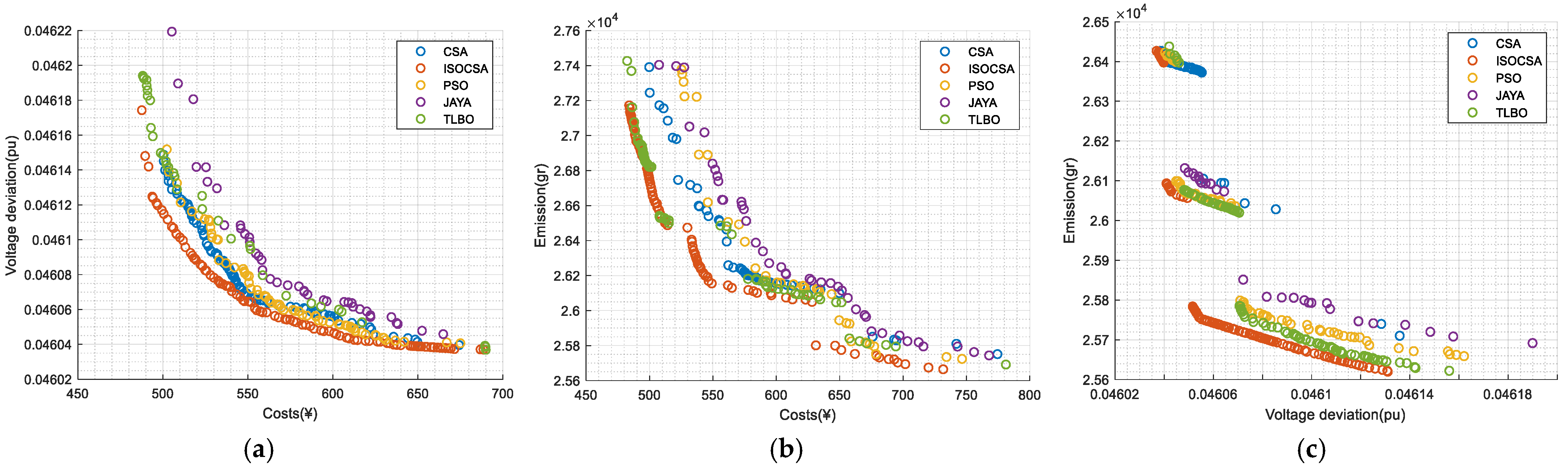
5.1.1. Evaluation of the Proposed Method

Initially, to analyze the algorithm’s effectiveness, the proposed algorithm has been applied to the model for only the most probable scenario with correlation, in both single and multi-objective states. The results of a single objective function for ISOCSA, where the mutation is applied to the crow’s memories rather than the repository (47), are compared with other algorithms.

Table 4. All functions’ comparison of the algorithms.

Function	Analysis	ISOCSA (fl = 1.5, α = 0.5)	ISOCSA (fl = 1.5, α = 1)	ISOCSA (fl = 1.5, α = 2)	ISOCSA (fl = 2, α = 0.5)	ISOCSA (fl = 2, α = 1)	ISOCSA (fl = 2, α = 2)	ISOCSA (fl = 2.5, α = 0.5)	ISOCSA (fl = 2.5, α = 1)	ISOCSA (fl = 2.5, α = 2)	CSA	PSO	JAYA	TLBO
f₁	Best	481.9568	481.9904	482.2295	482.144	482.4778	482.2312	483.3879	483.5854	484.3614	483.2319	487.1854	483.634	482.0054
	Worst	482.4872	483.2655	490.7695	491.4336	486.027	489.904	503.5032	497.2385	497.3467	484.3887	490.2728	485.766	482.713
	Median	482.3428	482.6224	483.3581	483.6339	483.7233	484.2281	487.9092	487.4907	487.5329	483.718	487.8968	484.4448	482.4149
	Std. Dev.	0.2012	0.2963	1.5692	1.6709	0.8692	1.4174	4.3039	3.9132	3.8889	0.2634	0.8523	0.4865	0.2025
f₂	Best	4.5368 × 10−2	4.5516 × 10−2	4.6012 × 10−2	4.5993 × 10−2	4.6096 × 10−2	4.6056 × 10−2	4.6236 × 10−2	4.6332 × 10−2	4.6525 × 10−2	4.6122 × 10−2	4.6937 × 10−2	4.6037 × 10−2	4.5851× 10−2
	Worst	4.6037 × 10−2	4.6070 × 10−2	4.7388 × 10−2	4.7571 × 10−2	4.6992 × 10−2	4.7232 × 10−2	5.1532 × 10−2	4.8332 × 10−2	4.8513 × 10−2	4.6598 × 10−2	4.7346 × 10−2	4.6711 × 10−2	4.6044 × 10−2
	Median	4.5722 × 10−2	4.5774 × 10−2	4.6623 × 10−2	4.6625 × 10−2	4.6471 × 10−2	4.6553 × 10−2	4.8978 × 10−2	4.7255 × 10−2	4.7471 × 10−2	4.6379 × 10−2	4.7152 × 10−2	4.6344 × 10−2	4.5936 × 10−2
	Std. Dev.	3.7667 × 10−8	2.0751 × 10−7	4.1080 × 10−7	9.1000 × 10−7	2.7971 × 10−7	2.8233 × 10−7	4.4051 × 10−4	1.8625 × 10−4	4.8919 × 10−5	1.6877 × 10−7	2.7962 × 10−7	2.7281 × 10−7	1.3505 × 10−7
f₃	Best	2.3587 × 104	2.3807 × 104	2.4325 × 104	2.4213 × 104	2.4379 × 104	2.4353 × 104	2.4728 × 104	2.4776 × 104	2.5385 × 104	2.4679 × 104	2.5786 × 104	2.4822 × 104	2.4141 × 104
	Worst	2.4106 × 104	2.4865 × 104	2.6224 × 104	2.6347 × 104	2.5841 × 104	2.6028 × 104	2.7078 × 104	2.6649 × 104	2.6701 × 104	2.5025 × 104	2.6523 × 104	2.5385 × 104	2.4506 × 104
	Median	2.3715 × 104	2.5262 × 104	2.5883 × 104	2.5918 × 104	2.5998 × 104	2.6046 × 104	2.6149 × 104	2.6005 × 104	2.6122 × 104	2.5921 × 104	2.6125 × 104	2.6061 × 104	2.5738 × 104
	Std. Dev.	123.1301	204.4091	238.8368	240.2564	222.1366	230.0278	422.4928	389.2940	255.5197	184.0515	218.6731	215.7913	151.1341

shows the values for the best, worst, mean, and standard deviation, which are derived from 30 executions of the algorithm and across various parameter settings for the proposed ISOCSA. Additionally, the maximum numbers of iterations and population size have been set to 5000 and 200, respectively. The results demonstrate that ISOCSA consistently outperforms the other algorithms in optimizing the three objective functions: cost ($f_1$), voltage deviation ($f_2$), and emissions ($f_3$).

For the cost objective ($f_1$), when fl and α equal 1.5 and 0.5, respectively, ISOCSA achieves the best result of 481.9568, which is lower than the best results of CSA (483.2319), PSO (487.1854), JAYA (483.634), and TLBO (482.0054). This configuration of ISOCSA also shows the smallest standard deviation of 0.2012, indicating high consistency in finding the most optimal solutions. The worst performance of ISOCSA with this configuration (482.4872) is still better than the best performance of the other algorithms, illustrating its robustness. In terms of voltage deviation ($f_2$) and emissions objective ($f_3$), the algorithm performs similarly to the cost objective ($f_1$) and preserves its superiority over other algorithms.

The analysis reveals that ISOCSA’s performance is sensitive to the choice of fl and α parameters. Generally, lower values of fl and α (particularly fl = 1.5 and α = 0.5) tend to yield better results across all three objectives. As these values increase, there is a trend towards slightly worse performance and higher standard deviations, indicating reduced consistency in finding optimal solutions. However, it is important to note that ISOCSA exhibits limitations under specific conditions. For example, Table 4 indicates that for higher values of fl and α (e.g., fl = 2.5 and α = 2), ISOCSA’s performance deteriorates, with higher standard deviations and less competitive results compared to CSA and TLBO for specific objectives such as voltage deviation (f₂). This degradation is primarily attributed to reduced exploitation capabilities and premature convergence to suboptimal solutions when the algorithm’s exploration is overly emphasized.

Additionally, while ISOCSA’s multi-objective performance typically results in a dominant Pareto front (as illustrated in Figure 3), scenarios involving highly complex and non-linear interactions between objectives may cause ISOCSA to struggle in maintaining diversity on the Pareto front. In such cases, algorithms like PSO and JAYA occasionally achieve better trade-offs for specific objectives due to their inherent balance between exploration and exploitation. This underscores the importance of fine-tuning algorithm parameters and understanding the problem’s characteristics when applying ISOCSA.

Overall, while ISOCSA demonstrates superior robustness and effectiveness in handling multi-objective optimization problems, acknowledging its limitations provides a more nuanced understanding of its performance, enabling informed decisions on its applicability to different scenarios.

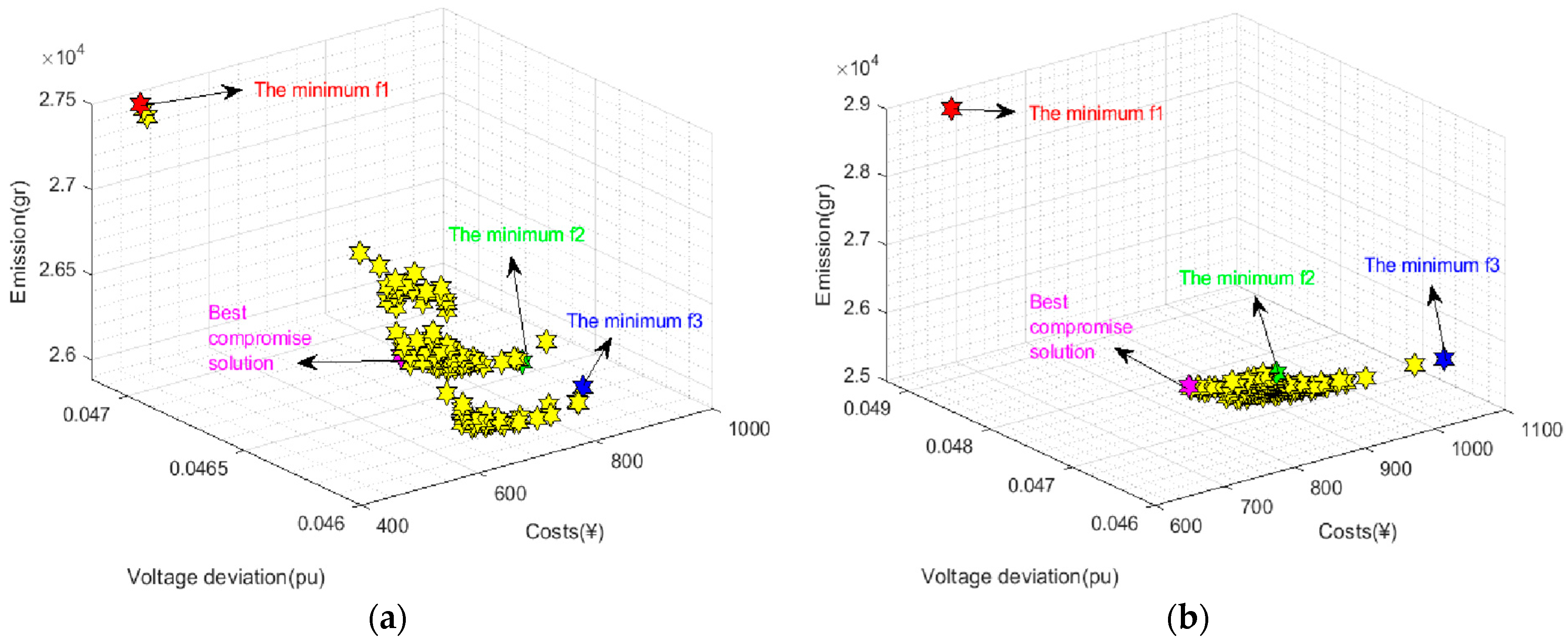
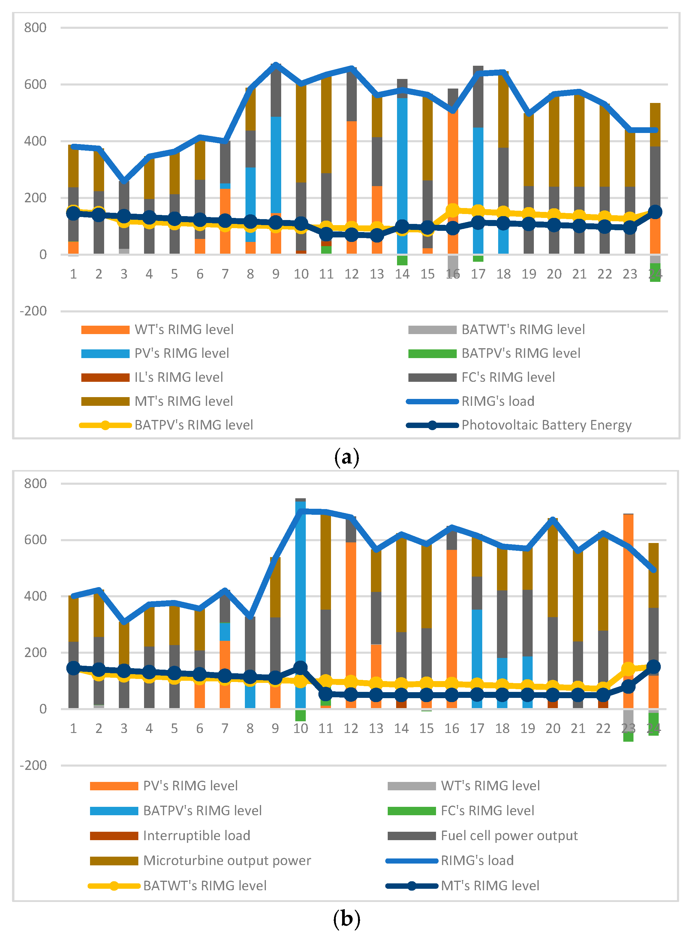
5.1.2. Results of the First Model

To address the multi-objective problem, all three objectives ($f_1$, $f_2$, and $f_3$) are considered. Figure 4 illustrates the Pareto front curves for the most probable scenarios both with and without correlation, using ${\omega }_n=0.33$ to identify the best compromise solution. The figure also presents the values for the best compromise solution and the minimum of each objective. Figure 5 shows the maximum output of each distributed power source in the RMG over a 24 h period and the maximum power discharged from electric energy storage devices under these scenarios. Additionally, Figure 6 demonstrates the DG results for the most probable scenario with and without correlation for the chosen best compromise solution on the Pareto front in Figure 4.

The assumptions regarding power consumption and IL curves for residential users significantly influence these results. These assumptions are based on typical residential load profiles, where peak loads occur during specific hours due to household activities. Consequently, the power balance and dispatch schedules are adjusted to meet these temporal variations. In scenarios with correlation, the stochastic dependencies between load, PV, and WT outputs are considered, leading to a more realistic representation of resource availability and usage. Without correlation, the independent treatment of these variables may lead to discrepancies, such as overestimation or underestimation of resource contributions.

For instance, in Figure 6b, which corresponds to the most probable scenario without correlation, observations at hour 14 reveal that despite the presence of PV output power, the load is supplied independently of PV units. This discrepancy arises because the minimum PV power required to meet the load exceeds the calculated output after considering the discard solar rate (1.9%) as per constraint (18). Even with excess power stored in the BAT associated with PV, an unutilized surplus remains, rendering solar power ineffective during this hour. This phenomenon also occurs from hours 11–13 and 15–16. However, in Figure 6a, which accounts for correlation, similar occurrences are observed but slightly shifted due to the interdependencies among variables, affecting the allocation of resources.

Fluctuations in BAT energy are minimal across both scenarios due to the high maintenance cost of BATs. BATs are charged only with their excess energy, and maintaining the energy level at hour 24 is a key constraint. This requirement necessitates either rescheduling energy allocation in prior hours or sourcing additional energy from the network. Such conditions are most evident for the WT’s BATs at hour 24, where insufficient WT output necessitates adjustments to ensure BAT energy returns to its initial value, as shown in Figure 6.

Table 5. Fuzzy Decision Making on the Pareto Front for the First Model.

Scenario		With Correlation			Without Correlation
		f1	f2	f3	f1	f2	f3
1	f1,min	1024.16	0.05089	29,466.86	1016.89	0.05007	27,629.38
	f2,min	1146.52	0.05082	28,871.58	1198.98	0.04943	26,520.63
	f3,min	1175.08	0.05087	28,438.98	1212.68	0.04949	26,268.10
	Best compromise solution	1026.07	0.05092	29,211.41	1055.92	0.04954	26,954.56
2	f1,min	548.20	0.04401	25,983.69	440.57	0.04169	23,911.64
	f2,min	747.27	0.04214	22,693.28	578.66	0.04149	23,502.80
	f3,min	986.73	0.04227	22,289.29	772.09	0.04165	22,721.67
	Best compromise solution	563.91	0.04235	23,442.24	440.57	0.04169	23,911.64
3	f1,min	573.26	0.04565	27,078.34	668.45	0.04701	28,346.14
	f2,min	759.22	0.04554	26,875.41	801.61	0.04691	27,975.56
	f3,min	1111.22	0.04585	26,150.10	1065.18	0.04712	26,977.99
	Best compromise solution	573.26	0.04565	27,078.34	693.80	0.04699	27,963.38
4	f1,min	481.99	0.04715	27,426.66	554.10	0.04793	29,159.79
	f2,min	689.90	0.04537	26,426.47	804.08	0.04716	27,856.34
	f3,min	908.34	0.04633	23,587.80	849.94	0.04726	26,833.79
	Best compromise solution	519.15	0.04613	26,565.07	582.21	0.04727	27,901.27
5	f1,min	702.30	0.04203	21,510.89	693.53	0.04927	28,744.74
	f2,min	1054.19	0.04173	20,695.99	818.38	0.04638	26,117.71
	f3,min	1202.06	0.04187	20,128.81	1079.01	0.04657	25,492.73
	Best compromise solution	702.30	0.04203	21,510.89	703.29	0.04647	26,203.15

summarizes the outcomes for various scenarios with and without correlation. It highlights significant variations in cost ($f_1$) and emissions ($f_3$) between scenarios. For example, in the third scenario with correlation, minimizing cost results in a value of CNY 573.26, whereas minimizing emissions yields a cost of CNY 1111.22, a 93.84% difference. Similarly, the emission values differ by 16.57% when minimizing cost compared to emission optimization. These variations emphasize the need for a multi-objective solution approach, as neglecting correlation can significantly impact the optimal trade-offs among objectives.

Furthermore, voltage deviation ($f_2$) differences are particularly noteworthy. The second scenario with correlation exhibits a 4.44% change, while the fifth scenario without correlation shows a 5.8% change. If a decision-maker sets a maximum permissible change of 6%, voltage deviation may be deprioritized when simultaneously considering cost and pollution emissions. Overall, these findings underscore the critical role of assumptions in shaping model results and the importance of accounting for stochastic interdependencies in RMG optimization.

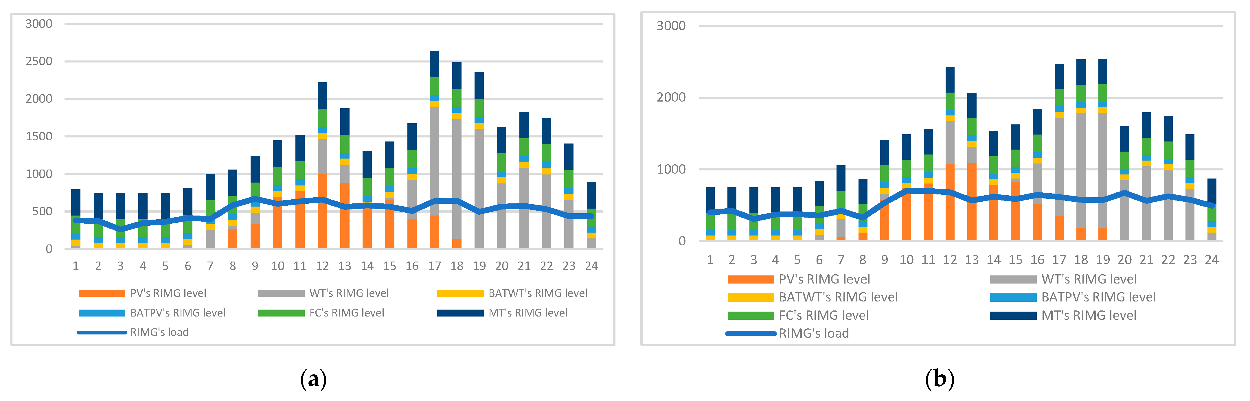
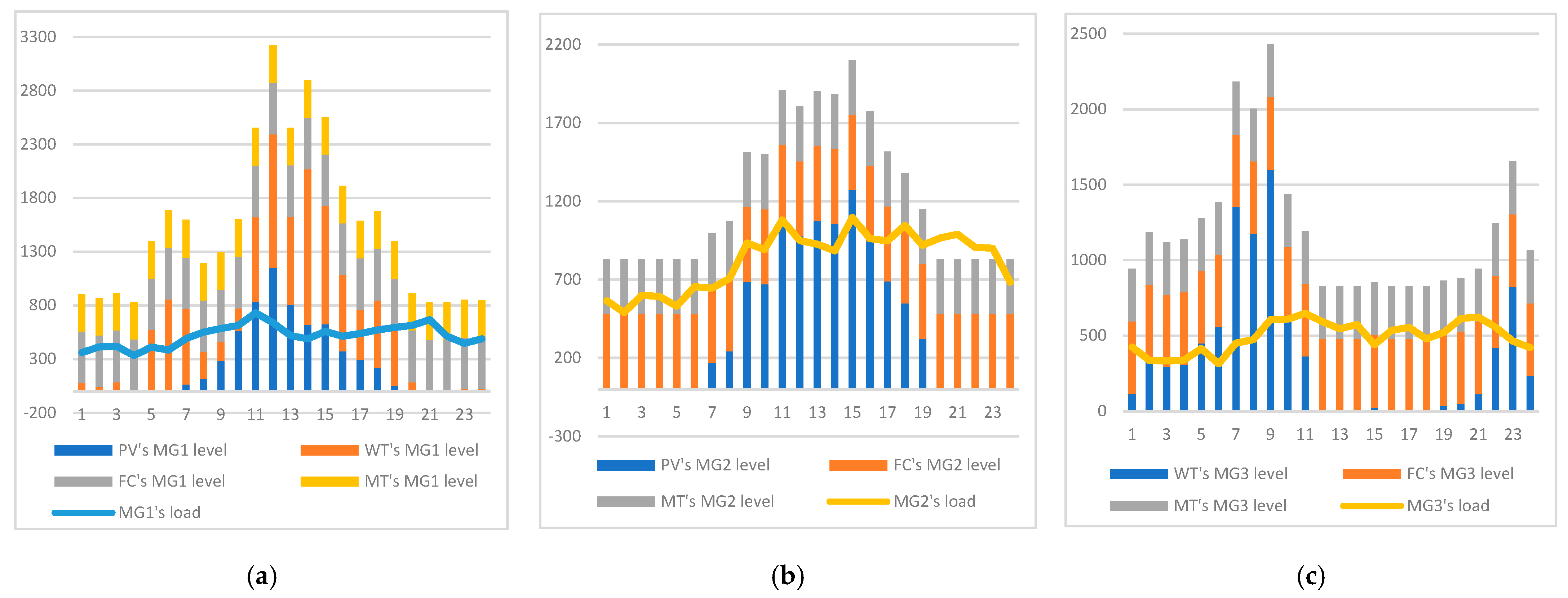
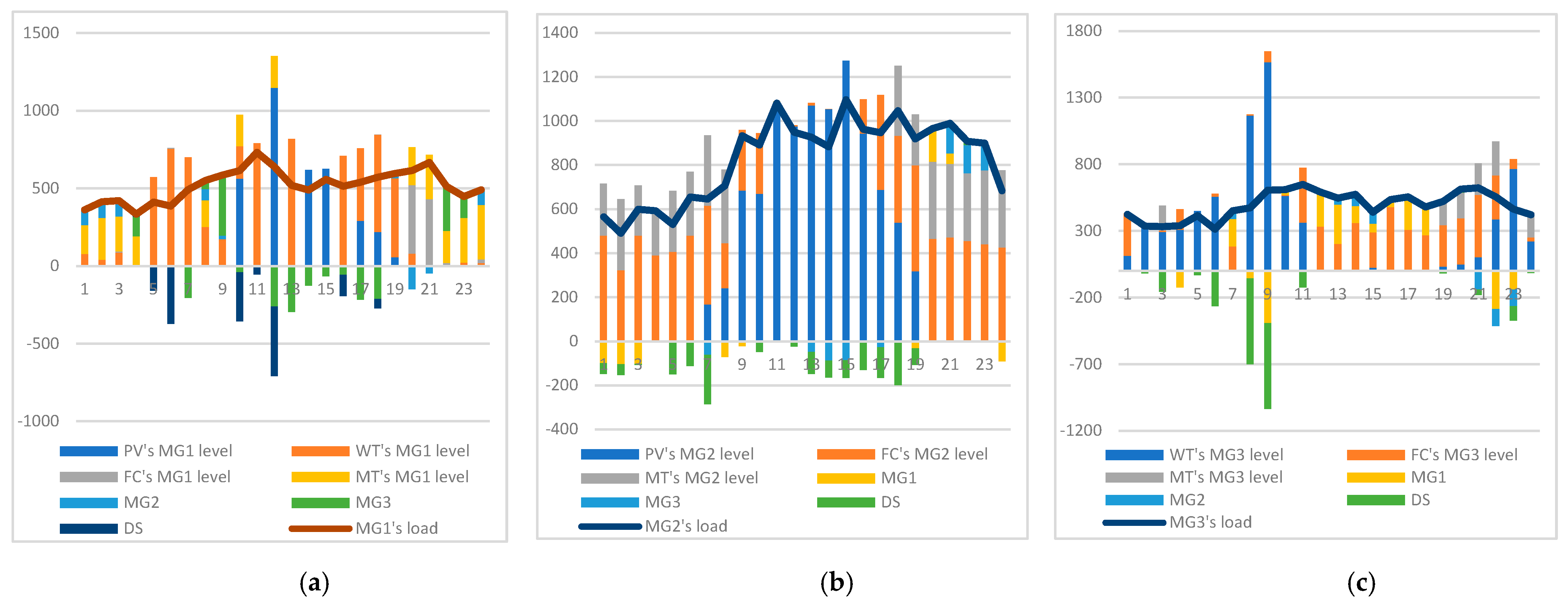
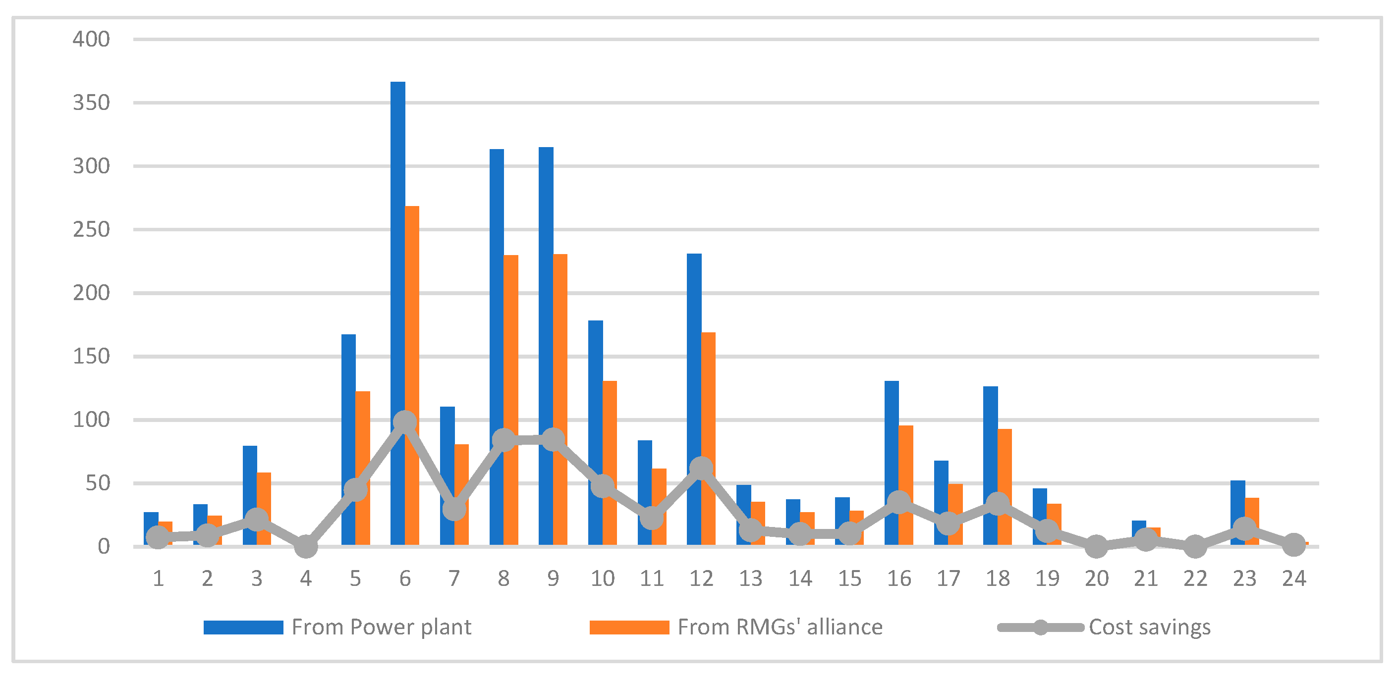
5.2. Results of the Second Model

RMGs, when operating conventionally, engage in power exchange solely with the distribution network.

Table 6. Fuzzy Decision Making on all Alliances for the Second Model.

Scenario	Form of Alliance	With Correlation			Without Correlation
		f1	f2	f3	f1	f2	f3
1	{MG1,MG2}	118.24	−0.00025	6827.9	270.59	0	9335.2
	{MG1,MG3}	65.6	−0.00025	13,183.9	16.2	0	2305.3
	{MG2,MG3}	196.41	0.00017	4209.3	302.55	−0.00023	7448.3
	{MG1,MG2,MG3}	197.94	0.00019	20,989.6	304.51	0.00017	13,993.9
2	{MG1,MG2}	282.5	0	6769.1	320.93	0.00002	8243.5
	{MG1,MG3}	78.79	0	9748.1	48.23	0.00002	10,616.9
	{MG2,MG3}	490.97	0	11,349.5	398.01	−0.00011	10,559.2
	{MG1,MG2,MG3}	567.59	0	24,009.8	413.05	0.000015	20,017.5
3	{MG1,MG2}	319.76	0.00024	8629.3	230.44	0.00044	9112.2
	{MG1,MG3}	−27.65	0.00024	12,763.8	22.45	0.00044	11,675.7
	{MG2,MG3}	367.79	0.00001	9430.1	264.79	0.00018	8665.6
	{MG1,MG2,MG3}	368.93	0.00025	22,447.8	266.46	0.00059	21,719.9
4	{MG1,MG2}	304.55	−0.00022	7932	147.77	0.00259	8460.04
	{MG1,MG3}	18.77	−0.00022	8969.3	50.45	0.00259	10,492.4
	{MG2,MG3}	381.4	−0.00021	11,760.8	180.95	0.00273	8287.7
	{MG1,MG2,MG3}	382.82	0.0008	21,206.6	182.44	0.00296	20,622.9
5	{MG1,MG2}	284.52	−0.00002	9451.1	232.61	0.00004	9788.8
	{MG1,MG3}	27.78	−0.00002	13,479.2	41.07	0.00004	11,286.5
	{MG2,MG3}	368.95	0.00003	9932.6	290.38	−0.00047	10,660.2
	{MG1,MG2,MG3}	370.35	0.00013	23,483.9	291.72	0.00014	22,838.5

depicts the variation between the optimized values under all feasible states of RMGs among generated alliances and their conventional operations. These differences are evaluated while the cost, emission, and voltage deviation are taken into account as the objective functions in selected scenarios.

Moreover, Table 6 indicates that when the objective function is either the optimization of cost or emission pollution regardless of whether the correlation is taken into account, the most optimal form of alliance across all scenarios is a full alliance. Moreover, when the objective is voltage deviation with or without correlation considering the unit’s capacity and load, the differences compared to the conventional operation are remarkably minimal, and the alliance form does not affect the optimization. Consequently, according to the presented results, the most favorable strategy for optimizing the cost, voltage deviation, and pollution emission is the formation of a full alliance, and the consideration of correlation does not influence the outcomes.

Figure 7 presents the maximum power generation values for RMGs and their corresponding loads under the most probable scenario with correlation. Figure 8 illustrates the power generation value associated with the best compromise solution from the resulting repository with ${\omega }_i$= 0.33 for the same scenario. As shown in Figure 7c, RMG3 does not generate sufficient wind output power from hours 12 to 18 to meet its load requirements, and under conventional operation, it must source this power from either the distribution network or its own MT and FC, which increases the cost and pollution.

However, as depicted in Figure 8c, after alliance generation by utilizing the excess power of RMG1 and RMG2 generated via their wind and solar units, both emission production and cost have been simultaneously reduced. Additionally, RMG3 has excess power from its WT unit at hour 23 while both RMG1 and RMG2 lack wind and solar output power. By transferring this excess power, both cost and pollution can be reduced. Therefore, the function of all three RMGs in energy provision and load management is complementary, and the alliance generation helps efficient energy planning to reduce both the cost and emission pollution.

Figure 9 and Figure 10 illustrate that it is more cost-effective and less polluting for the distribution network to purchase the surplus power from the RMG coalition than from the power plant. The cost-saving value is quantified at CNY 663.68, and the reduction in pollution emission is measured at 23,982.88 g.

6. Conclusions

MGs that integrate renewable power sources like PV and WT offer cost-effective and environmentally friendly energy alternatives. Hence, their utilization is particularly beneficial for rural communities. However, designing optimal scheduling for efficient generation is recognized as an important challenge. Therefore, in this paper, two distinct models, including an islanded mode and connection to the distribution network, were employed. They were utilized in rural areas in order to supply energy to consumers and optimize system performance along with reducing pollution emission, utilization of fossil fuels, and simultaneously increasing cost saving. The scientific novelty of this work lies in three key contributions: the development of IMOCSA that enhances optimization performance through adaptive chaotic awareness probability and mutation mechanisms, the introduction of a sophisticated scenario-based methodology incorporating correlations among uncertainties, and the presentation of a comprehensive two-model approach addressing both islanded and grid-connected operations. The practical significance is demonstrated through substantial reductions in operational costs and environmental impacts, with IMOCSA showing superior performance in handling multi-objective optimization, making it a valuable tool for system operators managing complex microgrid networks. Simulation results indicated that the coalition generation across all RMGs not only reduced operational costs and environmental impacts but also decreased the power purchasing cost from the power plant for the distribution network. These results have important implications for rural electrification projects, offering a practical framework for implementing cost-effective and environmentally sustainable power systems. Furthermore, we found that the correlation did not significantly influence the alliance results, which simplifies implementation for practical applications.

References

1. Islam, M.M.; Nagrial, M.; Rizk, J.; Hellany, A. General aspects, islanding detection, and energy management in Microgrids: A review. Sustainability 2021, 13, 9301. [Google Scholar] [CrossRef]
2. Dashtaki, A.A.; Hakimi, S.M.; Farahani, E.S.; HassanzadehFard, H. Simultaneous optimal location and sizing of DGs in distribution system considering different types of MGs in an electricity market. Multiscale Multidiscip. Model. Exp. Des. 2024, 7, 2443–2459. [Google Scholar] [CrossRef]
3. Rashwan, A.; Faragalla, A.; Abo-Zahhad, E.M.; El-Dein, A.Z.; Liu, Y.; Chen, Y.; Abdelhameed, E.H. Techno-economic Optimization of Isolated Hybrid Microgrids for Remote Areas Electrification: Aswan city as a Case Study. Smart Grids Sustain. Energy 2024, 9, 18. [Google Scholar] [CrossRef]
4. Bashir, A.A.; Pourakbari-Kasmaei, M.; Contreras, J.; Lehtonen, M. A novel energy scheduling framework for reliable and economic operation of islanded and grid-connected microgrids. Electr. Power Syst. Res. 2019, 171, 85–96. [Google Scholar] [CrossRef]
5. Han, Y.; Zhang, K.; Li, H.; Coelho, E.A.A.; Guerrero, J.M. MAS-based distributed coordinated control and optimization in microgrid and microgrid clusters: A comprehensive overview. IEEE Trans. Power Electron. 2017, 33, 6488–6508. [Google Scholar] [CrossRef]
6. Chen, G.; Wang, J.-M.; Yuan, X.-D.; Chen, L.; Zhao, L.-J.; He, Y.-L. Chinese national condition based power dispatching optimization in microgrids. J. Control. Sci. Eng. 2018, 2018, 8695391. [Google Scholar] [CrossRef]
7. Khan, M.R.; Haider, Z.M.; Malik, F.H.; Almasoudi, F.M.; Alatawi, K.S.S.; Bhutta, M.S. A Comprehensive Review of Microgrid Energy Management Strategies Considering Electric Vehicles, Energy Storage Systems, and AI Techniques. Processes 2024, 12, 270. [Google Scholar] [CrossRef]
8. Prinsloo, G.; Mammoli, A.; Dobson, R. Customer domain supply and load coordination: A case for smart villages and transactive control in rural off-grid microgrids. Energy 2017, 135, 430–441. [Google Scholar] [CrossRef]
9. Wang, Z.; Chen, B.; Wang, J. Decentralized energy management system for networked microgrids in grid-connected and islanded modes. IEEE Trans. Smart Grid 2015, 7, 1097–1105. [Google Scholar] [CrossRef]
10. Espín-Sarzosa, D.; Palma-Behnke, R.; Núñez-Mata, O. Energy management systems for microgrids: Main existing trends in centralized control architectures. Energies 2020, 13, 547. [Google Scholar] [CrossRef]
11. Sabzalian, M.H.; Pirouzi, S.; Aredes, M.; Franca, B.W.; Cunha, A.C. Two-Layer Coordinated Energy Management Method in the Smart Distribution Network including Multi-Microgrid Based on the Hybrid Flexible and Securable Operation Strategy. Int. Trans. Electr. Energy Syst. 2022, 2022, 3378538. [Google Scholar] [CrossRef]
12. Zhang, B.; Li, Q.; Wang, L.; Feng, W. Robust optimization for energy transactions in multi-microgrids under uncertainty. Appl. Energy 2018, 217, 346–360. [Google Scholar] [CrossRef]
13. Huang, B.; Li, Y.; Zhang, H.; Sun, Q. Distributed optimal co-multi-microgrids energy management for energy internet. IEEE/CAA J. Autom. Sin. 2016, 3, 357–364. [Google Scholar] [CrossRef]
14. Arefifar, S.A.; Ordonez, M.; Mohamed, Y.A.-R.I. Energy management in multi-microgrid systems—Development and assessment. IEEE Trans. Power Syst. 2016, 32, 910–922. [Google Scholar] [CrossRef]
15. Chen, F.; Wang, Z.; He, Y. A Deep Neural Network-Based Optimal Scheduling Decision-Making Method for Microgrids. Energies 2023, 16, 7635. [Google Scholar] [CrossRef]
16. Du, Y.; Li, F. Intelligent multi-microgrid energy management based on deep neural network and model-free reinforcement learning. IEEE Trans. Smart Grid 2019, 11, 1066–1076. [Google Scholar] [CrossRef]
17. Aguila-Leon, J.; Vargas-Salgado, C.; Chiñas-Palacios, C.; Díaz-Bello, D. Energy management model for a standalone hybrid microgrid through a particle Swarm optimization and artificial neural networks approach. Energy Convers. Manag. 2022, 267, 115920. [Google Scholar] [CrossRef]
18. Roldán-Blay, C.; Escrivá-Escrivá, G.; Roldán-Porta, C.; Dasí-Crespo, D. Optimal sizing and design of renewable power plants in rural microgrids using multi-objective particle swarm optimization and branch and bound methods. Energy 2023, 284, 129318. [Google Scholar] [CrossRef]
19. Zhang, X.; Son, Y.; Cheong, T.; Choi, S. Affine-arithmetic-based microgrid interval optimization considering uncertainty and battery energy storage system degradation. Energy 2022, 242, 123015. [Google Scholar] [CrossRef]
20. Tan, B.; Chen, H. Multi-objective energy management of multiple microgrids under random electric vehicle charging. Energy 2020, 208, 118360. [Google Scholar] [CrossRef]
21. Dev, A.; Mondal, B.; Verma, V.K.; Kumar, V. Teaching learning optimization-based sliding mode control for frequency regulation in microgrid. Electr. Eng. 2024, 106, 7009–7021. [Google Scholar] [CrossRef]
22. Liu, Y.; Yang, S.; Li, D.; Zhang, S. Improved whale optimization algorithm for solving microgrid operations planning problems. Symmetry 2022, 15, 36. [Google Scholar] [CrossRef]
23. Askarzadeh, A. A novel metaheuristic method for solving constrained engineering optimization problems: Crow search algorithm. Comput. Struct. 2016, 169, 1–12. [Google Scholar] [CrossRef]
24. Xu, Y.; Guo, Q.; Sun, H.; Fei, Z. Distributed discrete robust secondary cooperative control for islanded microgrids. IEEE Trans. Smart Grid 2018, 10, 3620–3629. [Google Scholar] [CrossRef]
25. Jia, Y.; Wen; Yan, Y.; Huo, L. Joint operation and transaction mode of rural multi microgrid and distribution network. IEEE Access 2021, 9, 14409–14421. [Google Scholar] [CrossRef]
26. Roustaei, M.; Niknam, T.; Salari, S.; Chabok, H.; Sheikh, M.; Kavousi-Fard, A.; Aghaei, J. A scenario-based approach for the design of Smart Energy and Water Hub. Energy 2020, 195, 116931. [Google Scholar] [CrossRef]
27. Christopher, S.B.; Mabel, M.C. A bio-inspired approach for probabilistic energy management of micro-grid incorporating uncertainty in statistical cost estimation. Energy 2020, 203, 117810. [Google Scholar] [CrossRef]
28. Atwa, Y.M.; El-Saadany, E. Optimal allocation of ESS in distribution systems with a high penetration of wind energy. IEEE Trans. Power Syst. 2010, 25, 1815–1822. [Google Scholar] [CrossRef]
29. Tabatabaee, S.; Mortazavi, S.S.; Niknam, T. Stochastic energy management of renewable micro-grids in the correlated environment using unscented transformation. Energy 2016, 109, 365–377. [Google Scholar] [CrossRef]
30. Biswas, P.P.; Suganthan, N.; Mallipeddi, R.; Amaratunga, G.A. Optimal reactive power dispatch with uncertainties in load demand and renewable energy sources adopting scenario-based approach. Appl. Soft Comput. 2019, 75, 616–632. [Google Scholar] [CrossRef]
31. Lins, D.R.; Guedes, K.S.; Pitombeira-Neto, A.R.; Rocha, A.C.; de Andrade, C.F. Comparison of the performance of different wind speed distribution models applied to onshore and offshore wind speed data in the Northeast Brazil. Energy 2023, 278, 127787. [Google Scholar] [CrossRef]
32. Elgamal, M.; Korovkin, N.; Elmitwally, A.; Menaem, A.A.; Chen, Z. A framework for profit maximization in a grid-connected microgrid with hybrid resources using a novel rule base-bat algorithm. IEEE Access 2020, 8, 71460–71474. [Google Scholar] [CrossRef]
33. Shen, J.; Jiang, C.; Liu, Y.; Wang, X. A microgrid energy management system and risk management under an electricity market environment. IEEE Access 2016, 4, 2349–2356. [Google Scholar] [CrossRef]
34. Talaat, M.; Elkholy, M.; Alblawi, A.; Said, T. Artificial intelligence applications for microgrids integration and management of hybrid renewable energy sources. Artif. Intell. Rev. 2023, 56, 10557–10611. [Google Scholar] [CrossRef]
35. Makhdoomi, S.; Askarzadeh, A. Optimizing operation of a photovoltaic/diesel generator hybrid energy system with pumped hydro storage by a modified crow search algorithm. J. Energy Storage 2020, 27, 101040. [Google Scholar] [CrossRef]
36. Gholami, J.; Mardukhi, F.; Zawbaa, H.M. An improved crow search algorithm for solving numerical optimization functions. Soft Comput. 2021, 25, 9441–9454. [Google Scholar] [CrossRef]
37. Shaheen, A.M.; El-Sehiemy, R.A.; Elattar, E.E.; Abd-Elrazek, A.S. A modified crow search optimizer for solving non-linear OPF problem with emissions. IEEE Access 2021, 9, 43107–43120. [Google Scholar] [CrossRef]
38. Song, X.; Lin, H.; De, G.; Li, H.; Fu, X.; Tan, Z. An energy optimal dispatching model of an integrated energy system based on uncertain bilevel programming. Energies 2020, 13, 477. [Google Scholar] [CrossRef]
39. Niknam, T.; Bornapour, M.; Gheisari, A.; Bahmani-Firouzi, B. Impact of heat, power and hydrogen generation on optimal placement and operation of fuel cell power plants. Int. J. Hydrogen Energy 2013, 38, 1111–1127. [Google Scholar] [CrossRef]
40. Zhang, J.; Hu, C.; Zheng, C.; Rui, T.; Shen, W.; Wang, B. Distributed peer-to-peer electricity trading considering network loss in a distribution system. Energies 2019, 12, 4318. [Google Scholar] [CrossRef]
Figure 1. Diagram of the first model.
Energies 18 00294 g001
Figure 2. Diagram of the second model.
Energies 18 00294 g002
Figure 3. Comparison of the Pareto front of the proposed algorithm and other algorithms. (a) Pareto front algorithms for costs and voltage deviation objectives. (b) Pareto front algorithms for emission and voltage deviation objectives. (c) Pareto front algorithms for costs and emission objectives.
Energies 18 00294 g003
Figure 4. Pareto front of the first model for multi-objective function. (a) Pareto front for the most probable scenario with correlation. (b) Pareto front for the most probable scenario without correlation.
Energies 18 00294 g004
Figure 5. Power load and generation level of the first model. (a) With correlation. (b) Without correlation.
Energies 18 00294 g005
Figure 6. Output optimization of the first model. (a) With correlation. (b) Without correlation.
Energies 18 00294 g006
Figure 7. Power load and generation level of the second model. (a) For MG1. (b) For MG2. (c) For MG3.
Energies 18 00294 g007
Figure 8. Outcomes of RMGs’ alliance operation. (a) For MG1. (b) For MG2. (c) For MG3.
Energies 18 00294 g008
Figure 9. Comparison of power purchasing cost for the distribution network.
Energies 18 00294 g009
Figure 10. Comparison of emission pollution for the distribution network.
Energies 18 00294 g010