Deep Learning Models Applied Flowrate Estimation in Offshore Wells with Electric Submersible Pump

Abstract

To address the persistent challenge of reliable real-time flowrate estimation in complex offshore oil production systems using Electric Submersible Pumps (ESPs), this study proposes a hybrid modeling approach that integrates a first-principles hydrodynamic model with Long Short-Term Memory (LSTM) neural networks. The aim is to enhance prediction accuracy across five offshore wells (A through E) in Brazil, particularly under conditions of limited or noisy sensor data. The methodology encompasses exploratory data analysis, preprocessing, model development, training, and validation using high-frequency operational data, including active power, frequency, and pressure, all collected at one-minute intervals. The LSTM architectures were tailored to the operational stability of each well, ranging from simpler configurations for stable wells to more complex structures for transient systems. Results indicate that prediction accuracy is strongly correlated with operational stability: LSTM models achieved near-perfect forecasts in stable wells such as Well E, with minimal residuals, and effectively captured cyclical patterns in unstable wells such as Well B, albeit with greater error dispersion during abrupt transients. The model also demonstrated adaptability to planned interruptions, as observed in Well A. Statistical validation using ANOVA, Levene’s test, and Tukey’s HSD confirmed significant performance differences (α < 0.01) among the wells, underscoring the importance of well-specific model tuning. This study confirms that the LSTM-based hybrid approach is a robust and scalable solution for real-time flowrate forecasting in digital oilfields, supporting production optimization and fault detection, while laying the groundwork for future advances in adaptive and interpretable modeling of complex petroleum systems.

1. Introduction

The accurate flowrate measurement is vital in the oil industry for operational control, performance assessment, and economic decision-making. Conventional devices such as Coriolis, ultrasonic, thermal, vortex, and turbine meters provide high precision but are costly, prone to failure in harsh conditions, and less effective in multiphase flows [1,2,3].

Among artificial lift methods for non-flowing wells, the Electrical Submersible Pump (ESP) is notable for its versatility, broad operational range, and ability to pressurize fluids for efficient transport to the surface at economically viable flowrates [4,5]. A complete ESP system integrates surface components, such as the power source, transformers, control panel, and wellhead, with subsurface equipment including the electric motor, protector, multistage pump, and power cables [6].

To effectively manage such systems and sustain production efficiency, precise and well-specific measurements remain critical. These data are essential for calibrating simulation models, estimating reserves, assessing decline rates, and optimizing the artificial lift performance [7,8,9].

The most advanced production systems using ESP, such as Phoenix CTS [10] or Welllift [11], allow the installation of sensors at the base of the motor. These sensors capture critical data, such as suction pressure, fluid temperature, and vibrations, which are transmitted to the surface via the motor’s electric cable. These data are essential for monitoring and automating operations but may be subject to failures due to adverse operational environment conditions [12]. This can lead to distorted monitoring signals and frequent false alarms [13].

A major challenge in ESP-based production systems is the dynamic variation in fluid properties inside the wellbore, caused by intense heat transfer between the high-temperature reservoir and the production fluids. According to [14], thermal effects in deep wells can significantly alter viscosity and filtration behavior by disrupting intermolecular hydrogen bonds. These changes generate a complex and nonlinear operating environment in which the relationship between pump power consumption and flow rate is unstable. Traditional mechanistic models, which assume fixed fluid properties, struggle to capture these dynamics, reinforcing the importance of data-driven approaches capable of learning such temporal patterns from operational data [14].

The data generated by sensors in production systems using ESP, such as pressure, temperature, and vibrations, have increased exponentially, requiring greater computational power for efficient processing and monitoring [15]. This scenario has driven the adoption of Industry 4.0 technologies, such as Big Data, the Internet of Things (IoT), cloud computing, and deep learning [16]. In fluid measurement for production systems, the application of deep learning and neural networks, particularly Long Short-Term Memory (LSTM) networks, has enabled more efficient data processing, enhancing monitoring and process automation [17]. Additionally, hybrid CNN-LSTM models have been used for forecasting sensor data, while CNN-MLP models classify potential faults in these measurements [18].

In the context of oil production, LSTM networks have stood out for their ability to model and predict flows, capturing temporal and spatial patterns in the data, improving precision and efficiency in production management. Various studies [19,20] have demonstrated the effectiveness of LSTM in predicting gas rates and multiphase production, while other studies [21] applied this technology to model complex flows in shale wells.

Recent research [22,23] has proven the superiority of LSTM compared to other models, such as DCA and XGBoost. Ref. [24] enhanced daily flow prediction using a combined CNN-LSTM network, while [25] utilized LSTM for detecting anomalous sensors in subsea production control systems. Other advancements include the use of BiLSTM, which has demonstrated greater accuracy and better generalization capability in complex shale gas production time series [26] and the development of hybrid networks, such as CNN-LSTM and BPNN-LSTM, which have improved prediction accuracy in MPD data [27].

The combination of hydrodynamic models with Long Short-Term Memory (LSTM) neural networks offers a more robust and effective approach for modeling and predicting liquid flow in production wells, especially in scenarios where sensor data transmission is restricted [28]. While hydrodynamic models, based on physical knowledge of fluids, may fail by not incorporating the stochastic structure of the data and relying heavily on data availability, LSTM, with its ability to capture autocorrelations and transient phenomena in time series, overcomes these limitations, enabling real-time analysis and improving productivity and decision-making in oil and gas production [29]. This integrated approach can also be incorporated into intelligent production systems, significantly contributing to the digital transformation process in the industry, especially in the development of virtual measurement tools that provide reliable results for optimized production management [30,31].

This study presents a hybrid method combining a first-principles hydrodynamic model with Long Short-Term Memory (LSTM) neural networks to estimate real-time oil flowrates in five offshore Brazilian wells using ESP systems. By integrating physics-based modeling with LSTM’s predictive capabilities, the approach overcomes limitations of purely mechanistic models. Results indicate accuracy depends on well stability, with strong performance in stable systems and effective cyclic behavior modeling in unstable ones. The method shows potential to improve real-time monitoring, productivity, and decision-making.

2. Materials and Methods

2.1. ESP Well FlowRate Estimation

In the wells analyzed in this study, all equipped with Electrical Submersible Pumps (ESPs), flowrates are measured using Coriolis-type multiphase flow meters (Emerson—Micro Motion, St. Louis, MO, USA). However, due to operational challenges and high instrumentation costs, production tests are conducted periodically (typically every 30 to 42 days) in compliance with regulatory guidelines [32]. To overcome these limitations, several flowrate estimation models have been developed based on hydrodynamic equations and artificial intelligence techniques. Notably, [33] proposed a model (Equation (1)) that estimates pump flowrate from electrical and pressure variables using a power balance. This equation establishes that the hydraulic power generated by the pump is proportional to the electrical power consumed by the motor, mediated by their respective efficiencies. The estimation of flowrate (Q_p) is derived as follows:

$${\displaystyle \frac{∆P·Q_p}{\mathrm{58,847}· {\eta }_p}}= {\displaystyle \frac{V_{m }·I ·PF · {\eta }_m · \sqrt{3}}{746}}$$

(1)

where $∆P$ is pump differential pressure (psi); $Q_p$ is flowrate (m³/day); ${\eta }_p$ is pump efficiency; $V_{m }$ is downhole motor voltage (V); $I$ is motor current (A); $PF$ is motor power factor and ${\eta }_m$ is motor efficiency. The unmeasured efficiency parameters (${\eta }_p$ and ${\eta }_m$) were quantified by adopting the nominal efficiency values provided by the equipment manufacturer at the Best Efficiency Point (BEP). This assumption provides a robust baseline estimate for periods of stable operation, although it is acknowledged that real-time efficiencies vary with operational conditions.

The hydrodynamic model assumes that the pump’s hydraulic power equals the motor’s electrical input, mediated by system efficiencies. These efficiencies were estimated from pump and motor performance curves suited to the equipment scale and flowrates of the wells. However, efficiencies are not constant: motor efficiency increases with flowrate until stabilizing, while pump efficiency can degrade over time, usually detected in well tests. For these reasons, fixed efficiencies were adopted as a primary simplification of the model. To improve real-time flowrate estimation and minimize reliance on sensors, the authors also proposed an alternative equation to estimate the theoretical maximum flowrate, based on active power and performance at the best efficiency point (BEP), is shown in Equation (2):

$$q=q_{max} · {\displaystyle \frac{f}{60}} \left[1- {\displaystyle \frac{q_{max} · ∆P}{\sqrt{3 } ·V_m ·I_f ·cos\phi · {\eta }_m ·4{\eta }_b^{BEP}}} · \left({\displaystyle \frac{f}{60}}\right)\right]$$

(2)

where $q_{max}$ is maximum flowrate (m³/day); $f$ is operating frequency (Hz); ${\eta }_b^{BEP}$ is pump efficiency at BEP and $V_m, I_f, cos\phi , {\eta }_m$ are electrical and efficiency parameters. These were determined through multivariate regression analysis using historical data from periodic production tests. This calibration process is essential to tune the generalized model to the unique performance characteristics of each well’s specific downhole equipment and reservoir interactions, thus ensuring the model’s practical applicability.

This approach requires pump/motor performance curves and discharge pressure data from sensors or multiphase correlations. Purely physical models overlook operational variability, limiting predictive value [34]. We propose a hybrid method integrating hydrodynamic modeling with deep learning, trained on historical datasets to detect patterns even with partial sensor loss. Variable normalization prevents numerical instability, and time-series features enhance forecast accuracy.

ESP operation in multiphase offshore wells faces challenges from free gas, which reduces pump efficiency, impairs motor cooling, and accelerates wear [35,36]. Gas separators help, but regime shifts, such as bubble-to-slug flow, still degrade performance. Advances in Virtual Flow Metering (VFM) highlight hybrid models’ potential, yet machine learning applications remain limited, especially for uncertainty quantification [37]. The system’s nonlinearity, from viscosity and flow regime changes, hinders universal model development [38].

2.2. Workflow

The methodology of this study consisted of six sequential phases (Figure 1): Problem Identification (and scope delineation), Data Obtaining (acquisition of operational well data with provenance documentation), Data Exploration (preprocessing and feature extraction), Data Preparation, Model Selection, and Model Validation.

The study began by defining the problem to evaluate the feasibility of integrating hydrodynamic modeling with deep learning for real-time oil flowrate estimation in wells with Electric Submersible Pumps (ESPs) (Baker Hughes, Houston, TX, USA). Operational well data were collected with careful attention to provenance and acquisition conditions to ensure model robustness. Hydrodynamic modeling supported the extraction of relevant physical variables, which were then used to select a deep learning architecture suited to the data’s temporal and nonlinear patterns. Model validation employed statistical metrics to confirm predictive accuracy. The results demonstrated that the hybrid approach can deliver reliable real-time flowrate estimates, offering potential for improved petroleum production efficiency.

2.2.1. Problem Identification

Precise flowrate measurement in oil wells, particularly offshore, remains a significant challenge. Conventional physical sensors often face reliability issues due to extreme pressure, temperature, and multiphase flow conditions. Consequently, sensor failures, noise, and technical limitations directly compromise real-time monitoring and production management [25]. As a critical economic and operational parameter, accurate flowrate estimation is essential for ensuring production continuity, safety, and profitability [39].

This study investigates deep learning models, specifically Long Short-Term Memory (LSTM) neural networks, for predicting liquid flowrates in offshore production wells. The research focuses in five offshore wells located in Northeast and Southeast Brazil, all utilizing Electric Submersible Pump (ESP) artificial lift systems. LSTM networks demonstrate particular effectiveness in this application due to their ability to: (1) capture long-term temporal patterns in operational data, (2) maintain robust performance with noisy or incomplete datasets, and (3) provide reliable estimates even during periods of sensor unavailability [18,20,29].

2.2.2. Data Obtaining

The data acquisition and preparation phase constituted a fundamental stage of this research, involving systematic collection and processing of operational parameters from five offshore wells equipped with Electric Submersible Pump (ESP) systems. The dataset included critical variables such as active power, operating frequency, suction pressure, and wellhead pressure, recorded at one-minute intervals through the PI Datalink tool integrated with Microsoft Excel. As shown in

Table 1. Distribution of collected data records by well.

Well	Number of Records
A	59,021
B	40,320
C	61,282
D	61,282
E	61,282

, the volume of data collected showed variations between 40,320 and 61,282 points in different wells.

The data processing workflow was implemented in Python (3.12) using Google Colab, chosen for its efficient resource management and support for reproducible analysis. To ensure confidentiality, all well identifiers were anonymized (A through E). The dataset’s high temporal resolution (1 min intervals) was crucial for capturing transient phenomena essential for time-series modeling. Building on the established work of [33], the methodology was adapted to address variable data volumes across wells, providing a robust foundation for subsequent deep learning and predictive modeling.

2.2.3. Data Exploration

The data exploration phase is crucial for ensuring data quality in predictive modeling, enabling the detection of patterns, inconsistencies, and key relationships. In this study, exploratory analysis was conducted after data acquisition to compare the hydrodynamic model’s flowrate estimates with regulatory-compliant well test measurements. This process identified sensor failures, operational deviations, and other issues affecting data integrity. Graphical tools, statistical metrics, and Pearson’s correlation analysis were applied to all five offshore wells, supporting the identification of production trends, anomalies, and inter-parameter relationships, and providing a solid foundation for subsequent model development and validation.

2.2.4. Data Preparation

The data preparation procedure was designed to enhance both accuracy and consistency of the dataset. Inactive well periods were excluded to achieve standardized sample sizes, and spurious negative flow rate values were removed. Missing data were not corrected using interpolation techniques such as linear or spline fitting, in order to avoid artificial signal distortion. Instead, anomalous or absent entries, most often linked to sensor malfunctions in pressure or frequency measurements, were systematically replaced with zero values, ensuring uniformity across the dataset. Normalization was applied to address scale disparities, while outlier detection combined statistical thresholds with domain knowledge. Imputation techniques for missing values were chosen to preserve critical temporal dependencies. Finally, the dataset was partitioned into training (70%) and testing (30%) subsets to ensure robust model validation.

This rigorous processing yielded a representative sample of real offshore well operating conditions (Table 1 with base dataset), establishing a solid foundation for subsequent modeling. Such a comprehensive approach is essential for enhancing model reliability when handling the noisy and incomplete data characteristic of offshore environments, ensuring that predictive systems are built upon a clean, consistent, and representative operational foundation.

2.2.5. Model Selection

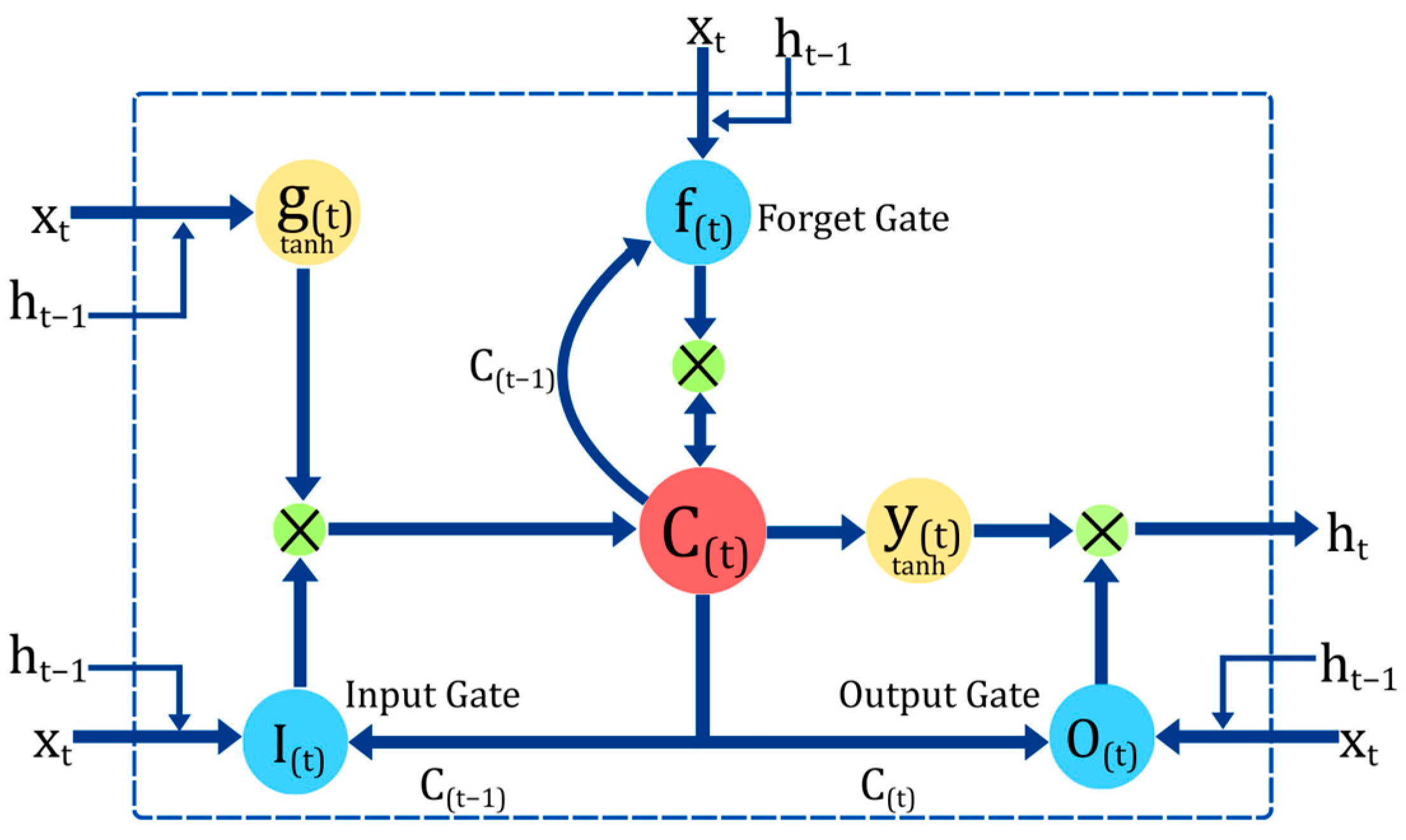
Deep learning (DL) has become central to data-driven modeling in complex systems, offering advanced capabilities for analyzing sequential data [40,41]. While traditional recurrent neural networks (RNNs) are designed for this purpose, they are often limited by an inability to capture long-range temporal dependencies due to issues like the vanishing gradient problem [42,43]. To overcome this, the Long Short-Term Memory (LSTM) network was developed as a specialized RNN architecture. LSTMs are defined by their unique structure, which incorporates gated mechanisms (input, forget, and output gates) that regulate the flow of information. This allows the network to selectively retain relevant patterns over extended time steps, making it highly effective for modeling time series with long-term dependencies [43,44].

Given these strengths, LSTMs are increasingly applied in industrial contexts such as predictive maintenance and, specifically within oil and gas operations, for forecasting flowrates and detecting equipment malfunctions [15,25,26,41]. The selection of the LSTM model for this study was motivated by its proven effectiveness in predicting production variables in multiphase systems and its suitability for the dataset obtained from the offshore wells. These data consist of highly variable and nonlinear multivariate time series (including active power, frequency, and pressures), where the LSTM’s ability to preserve temporal memory is crucial for identifying latent patterns associated with operational failures or flow rate fluctuations [19,20,21,22,23,41].

To optimize the model’s performance and mitigate known limitations such as high computational cost and risk of overfitting, the architecture was enhanced with regularization techniques, including dropout and early stopping [45]. The Adam optimizer was also employed for its computational efficiency in large-scale settings. At the core of this architecture is the LSTM cell, which functions like a “conveyor belt” for information, using its gated mechanisms to carry relevant signals across numerous time steps without degradation [41,46,47]. This structure, which combines the LSTM cell with specific optimization and regularization methods to effectively model the dynamic behavior of well operations, is detailed in Figure 2.

An LSTM cell’s gating mechanism allows it to identify, store, and retrieve information, enabling it to effectively capture long-range dependencies in temporal data. For this study, each well’s LSTM was customized based on data quality and validation performance, measured by Mean Squared Error (MSE).

The models were implemented in Python (3.12) using Keras (3.3) [48], with data management handled by Excel and the Pandas library (3.0). Key hyperparameters, including learning rate, layers, neurons, and dropout rate, were optimized through iterative experimentation, as detailed in

Table 2. Hyperparameters of each applied LSTM model.

Model.	Hyperparameters	Conditions
LSTM	Activation	Linear, Tanh and Relu
	Alpha	{0.01; 0.005}
	Hidden_layer_sizes	{(32:32:16), (64:64:32), (128:64:64)}:
	Learning_rate	Constant, Adaptive and Invscaling
	Learning_rate_init	{0.001; 0.005}
	Solver Dropout	Sgd and Adam 0.20 and 0.30

.

The hyperparameter selection was performed using a trial-and-error method. This process involved testing values in multiples of 8 (e.g., 16, 32, 64), in accordance with the recommendations in the literature [49,50].

In summary, the use of LSTM enabled the development of effective predictive models for real-time flowrate estimation, even under complex operational conditions. Integrating this approach with industrial sensor data streams paves the way for future applications in smart field systems, contributing to improved operational efficiency, reduced corrective maintenance costs, and enhanced decision-making in the oil and gas industry.

2.2.6. Model Validation

The performance of machine learning and deep learning models, including LSTM, depends heavily on the proper selection of hyperparameters. These predefined settings influence both the model architecture and its ability to generalize. Key hyperparameters include the optimizer, evaluation metric (e.g., Mean Squared Error), number of hidden layers, neurons per layer, learning rate, and activation functions. When properly tuned, these parameters significantly enhance model performance by adapting the architecture to the specific characteristics of the dataset.

In addition to hyperparameter tuning, this study employed regularization techniques to prevent overfitting and improve model generalization. Specifically, L1 (lasso), L2 (ridge), and dropout were applied. L1 and L2 add weight penalties to the loss function, encouraging sparsity and stability, respectively, while dropout randomly deactivates neurons during training, promoting robustness and reducing reliance on specific features.

In the modeling process, the liquid flowrate (m³/day), estimated from active power, operating frequency, and suction/discharge pressures, was the main predictive target. Calculations followed [33], using one-minute interval data from two offshore wells. LSTM-based modeling was chosen for its ability to capture long-term temporal patterns and complex variable dependencies.

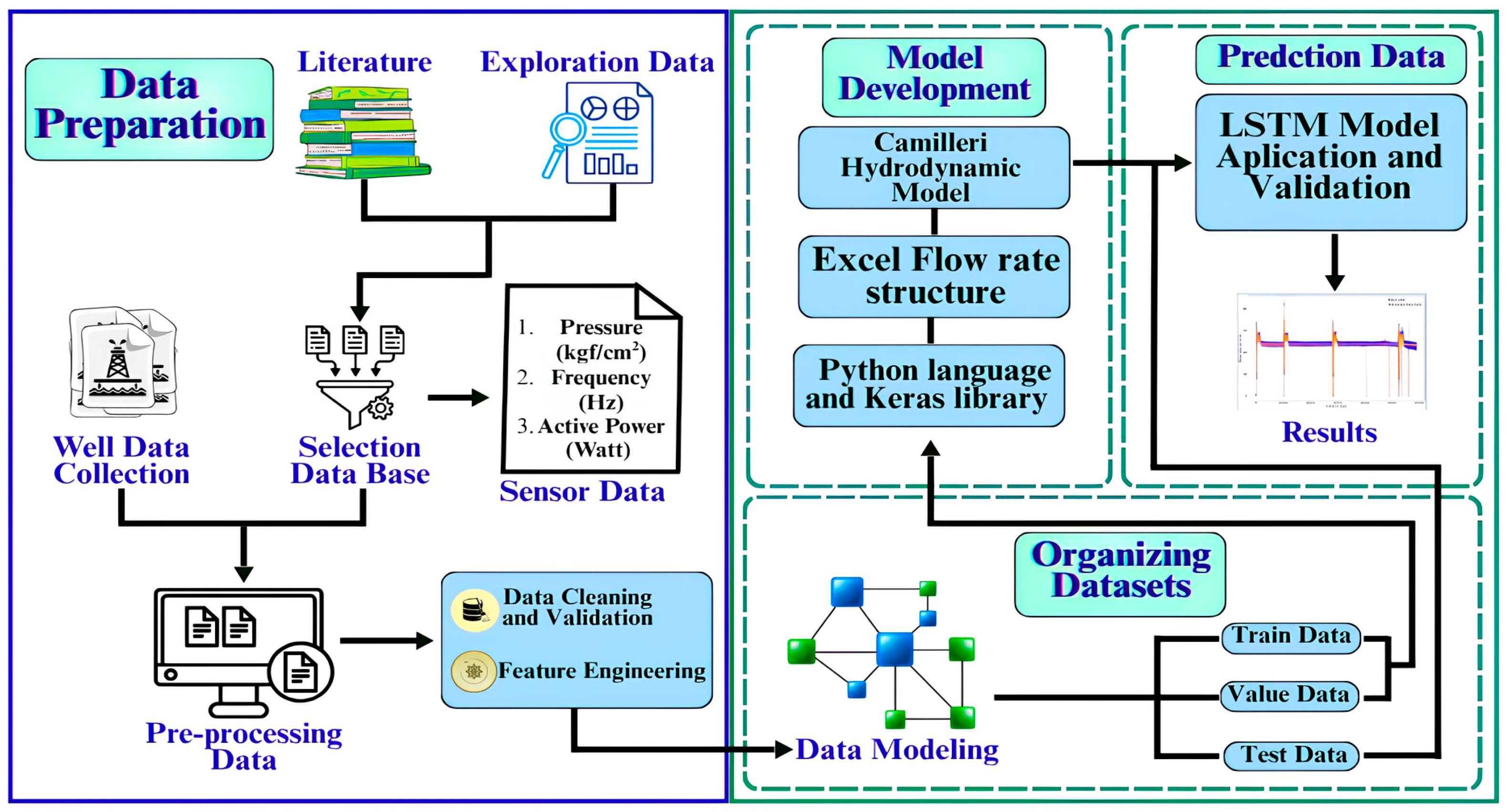
To ensure robustness, the data were split into training (70–90%) and test sets, with cross-validation and early stopping applied to prevent overfitting. Model performance was assessed using Mean Squared Error (MSE) for both sets, selecting configurations that minimized errors and maintained stability. These practices reinforced the accuracy and applicability of LSTM models in complex industrial contexts, such as oil and gas. Figure 3 presents the workflow employed in the study.

The complete workflow adopted in this study is structured in three main stages: data preparation, model development, and prediction. The process begins with the collection of well data and relevant literature, followed by the selection and preprocessing of key sensor variables, namely pressure, frequency, and active power. These variables undergo data cleaning, validation, and feature engineering to ensure quality and consistency. Subsequently, data modeling incorporates a hydrodynamic framework (Ref. [33] model) and is implemented using Excel-based flowrate structures and Python (3.12) with the Keras library (3.3). The processed datasets are then organized into training, validation, and testing subsets. Finally, the LSTM model is applied and validated, producing real-time flowrate predictions and performance results.

3. Results

3.1. Exploratory Data Analysis

This section details the exploratory data analysis of key operational variables, including well flowrate, pump head pressure, suction pressure, power consumption, and operating frequency. Individual and joint analyses across Wells A–E identified patterns and correlations to inform subsequent modeling.

3.1.1. Results of Well A

An exploratory data analysis for Well A was performed on key operational variables, including active power, frequency, suction and wellhead pressures, and the flowrate estimated from the hydrodynamic model by [33]. These variables were examined using detailed graphical representations to evaluate their temporal behavior and interrelationships. This analysis is critical, as the behavior of these parameters directly impacts predictive model performance and aligns with the physical relationships in the referenced hydrodynamic framework. Figure 4 and Figure 5 present this detailed graphical analysis for Well A.

Figure 4 presents the temporal behavior of critical operational parameters for Well A, including active power, frequency, suction pressure, and head pressure. The data demonstrate characteristic patterns of operational stability, with clearly distinguishable periods of steady-state production interspersed with brief interruptions attributable to operational interventions. These transient events are consistently followed by rapid system recovery, indicating robust operational management protocols.

The active power profile (Figure 4a) exhibits remarkable stability during normal operation, maintaining values between 20 and 22 kW, which confirms consistent electrical supply to the pumping system. The observed sharp declines to near-zero values represent controlled shutdown events, likely implemented as part of pressure management protocols or maintenance procedures. The immediate restoration of power levels following these events suggests an automated protection system is effectively maintaining operational integrity.

Frequency measurements (Figure 4b) directly correlate with the active power behavior, demonstrating stable operation at approximately 55 Hz during production periods. The synchronous drops in frequency with power interruptions confirm coordinated system shutdowns. The precise maintenance of target frequency during active periods indicates excellent regulation by the variable frequency drive (VFD) and stable power supply conditions.

Suction pressure dynamics (Figure 4c) reveal characteristic operational signatures, with baseline values around 40 kgf/cm² during normal flow conditions. The dramatic pressure surges exceeding 80 kgf/cm² during shutdown periods represent expected hydrodynamic responses to flow interruption, where reservoir energy accumulates at the pump intake. The consistent return to baseline values following system restart demonstrates effective pressure management.

Head pressure measurements (Figure 4d) show stable operation within the 6–8 kgf/cm² range, indicating proper downstream flow control. The absence of extreme pressure excursions during shutdown events suggests effective pressure dissipation mechanisms in the delivery system. The minor pressure fluctuations observed during system restart represent normal transient behavior as the pump re-establishes equilibrium between suction and discharge conditions.

Collectively, these parameters paint a comprehensive picture of Well A’s operational profile, characterized by extended periods of stable production punctuated by brief, controlled interruptions. The system’s rapid recovery following these events and the maintenance of all parameters within expected operational ranges demonstrate effective field management practices and robust equipment performance. This behavior pattern is consistent with modern production wells employing automated protection systems and routine maintenance protocols. The data quality and consistency support their use for further analytical modeling and performance optimization studies.

The flowrate data from Well A, presented in Figure 5, exhibits characteristic operational patterns that merit detailed examination. The temporal profile demonstrates stable production conditions with flowrates consistently maintained within a well-defined operational range, punctuated by periodic interruptions. During normal operation, the flowrate stabilizes around 50 m³/d, reflecting optimal reservoir deliverability and pump performance. The observed fluctuations show an amplitude of approximately ±10–15%, indicating moderate but expected variability in production conditions.

Sharp drops to zero flow are observed at regular intervals, approximately every 18,000 to 20,000 min, typically lasting 1000 to 1500 min. These patterns suggest planned shutdowns for operational maintenance or pressure control. Each interruption is followed by a rapid recovery to baseline production levels, indicating effective restart protocols. The absence of gradual decline prior to these events reinforces the interpretation of controlled, non-emergency shutdowns.

Moreover, the stability of flowrates between shutdown events reflects consistent reservoir pressure support and effective operation of the artificial lift system. This behavior is consistent with established production management practices in which periodic interruptions are employed to preserve long-term well integrity and maximize well recovery performance following operational interruptions. The high quality of the data, demonstrated by clear signal continuity and the absence of measurement artifacts, provides a robust and reliable foundation for subsequent production analyses and predictive modeling.

3.1.2. Results of Well B

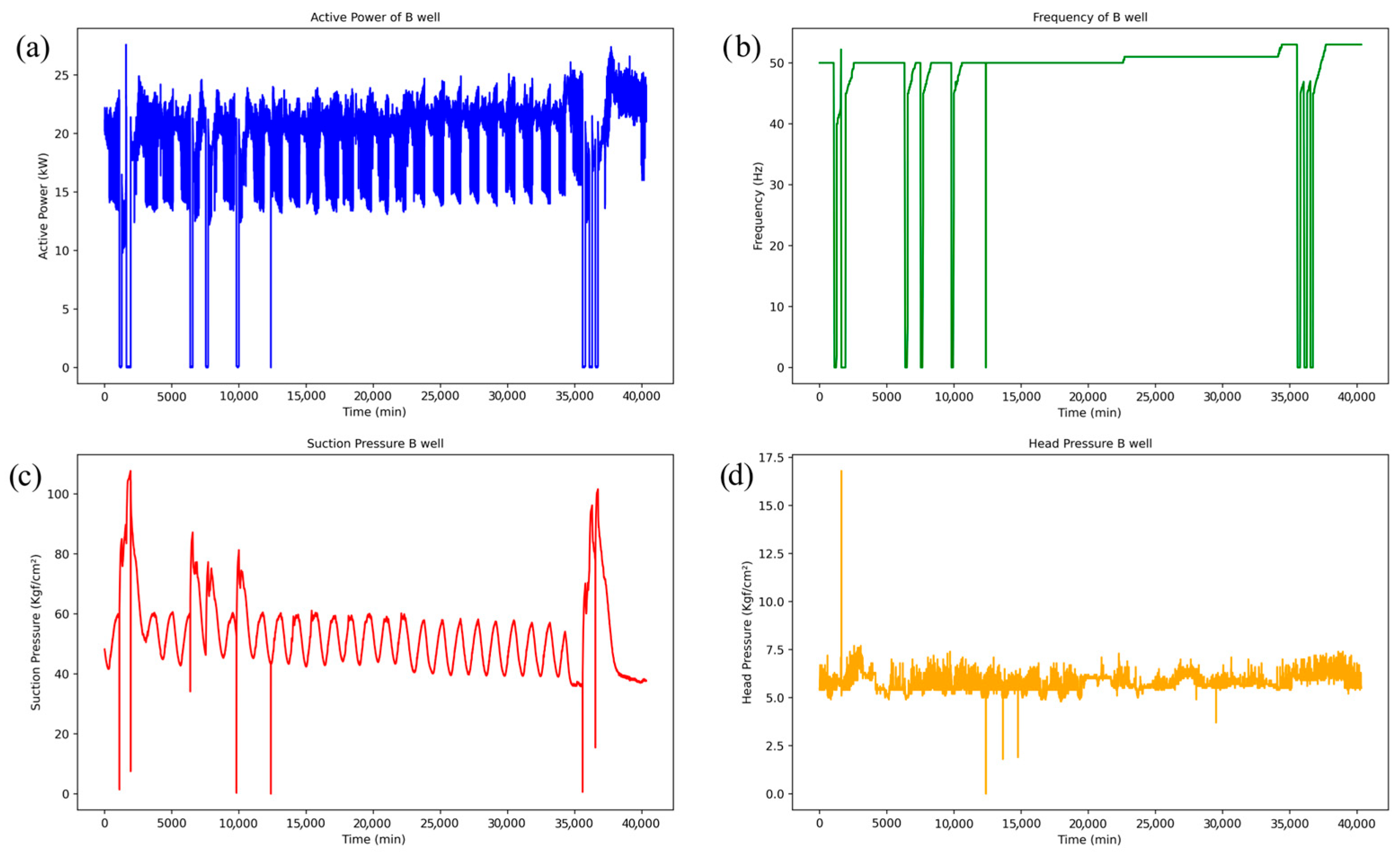
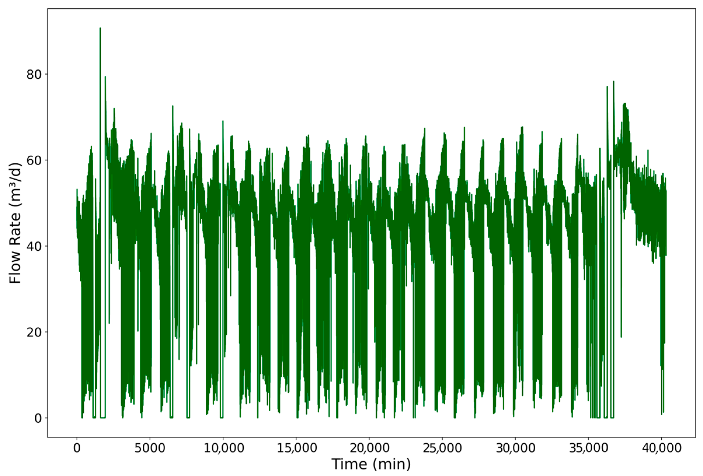
Figure 6 and Figure 7 present the operational variables for Well B, which exhibit a markedly different behavior compared to Well A. While Well A’s operation is characterized by relative stability, Well B demonstrates significant operational instability, as evidenced by cyclical fluctuations in its data.

The wellbore configuration for Well B features a packer set below the Electric Submersible Pump (ESP), with a 350 m lower tubing section extending further downhole. The prevailing hypothesis suggests that gas accumulates in the lower section of the tubing annulus. Periodically, this trapped gas is believed to reach the intake of the production tubing below the packer. Such an event would cause a rapid increase in the gas volume fraction at the pump’s suction, consequently impairing its performance. This phenomenon provides a compelling explanation for the cyclical patterns observed in Well B’s pressure, power, and production data, which manifest with a consistent periodicity, particularly upon pump startup.

The operational behavior of Well B, detailed in the accompanying figures, presents a stark contrast to the stable conditions observed in Well A. The time-series data for active power (Figure 6a), frequency (Figure 6b), suction pressure (Figure 6c), and head pressure (Figure 6d) collectively illustrate an operation characterized by severe instability and periodic cycles. The active power exhibits pronounced fluctuations, which correspond directly to extreme volatility in the suction pressure. Crucially, the frequency plot reveals that these unstable periods culminate in repeated, systematic shutdowns of the pump, where the operational frequency drops to 0 Hz before restarting. This pattern confirms that the well operates under transient conditions, a behavior that directly results in the cyclical flowrate presented in Figure 7.

The production flowrate of Well B, as illustrated in the provided figure, is characterized by significant instability and severe transient behavior. The data clearly shows a distinct cyclical pattern where production periodically ceases entirely, with the flowrate dropping to zero m³/d. During the operational phases between these interruptions, the flowrate remains highly volatile, fluctuating rapidly within a wide band, generally between approximately 40 and 70 m³/d. This cyclical start–stop behavior, which persists with a consistent periodicity throughout the monitored timeframe, confirms a non-steady-state production regime and highlights profound operational challenges for this well.

The presence of these severe, transient operational states is of particular importance to this study for two main reasons. First, such challenging conditions serve as a rigorous test for assessing the robustness and predictive accuracy of the proposed LSTM network. A model that performs effectively under these adverse real-world dynamics demonstrates strong potential to support production management and enhancing operational decision-making. Second, this scenario highlights the capability of the hybrid modeling approach to generate accurate forecasts even when physical sensors might fail or provide erroneous readings, as long as the well remains operational. This ability to maintain predictive oversight during intermittent sensor failure is critical for ensuring operational continuity and enabling proactive intervention.

3.1.3. Results of Well C

Wells C–E are completely different from wells A and B. They have only two things in common: they are offshore wells and equipped with ESP. While wells A and B are located in the Northeast region of Brazil, wells C–E are located in the Southeast region of Brazil. In addition, wells A and B have reduced oil and gas production with several operational problems. Wells C–E, on the other hand, have high production and high efficiency, with rare shutdowns, and it can be said that there is a team of engineers working preventively to avoid failures and production shutdowns.

The graphs below and the following sections show results from wells C–E that differ greatly from the results seen so far from wells A and B. Consistent with the analysis performed on the preceding wells, an exploratory data analysis was conducted for Well C. This analysis encompassed the primary operational variables: active power, operating frequency, suction pressure, wellhead pressure, and flowrate. Figure 8 and Figure 9 provide a detailed graphical representation of these data.

The graphs in Figure 8 show the behavior of key operational parameters for Well C: active power (Figure 8a), frequency (Figure 8b), suction pressure (Figure 8c), and head pressure (Figure 8d). The data indicate a system operating predominantly under stable conditions, with occasional interruptions likely due to planned events or transient disturbances.

Active power (Figure 8a) remains stable around 1000 kW, reflecting a high-capacity pumping system with consistent energy input. Five distinct drops to nearly zero occur, typical of automated safety shutdowns, scheduled maintenance, or brief power losses. Their short duration and rapid recovery suggest controlled stoppages rather than equipment failures.

Frequency (Figure 8b) closely follows the power trend, staying near 53 Hz during normal operation. Reductions in frequency coincide with power drops, confirming the pump’s variable frequency drive was off or reset. The near-constant frequency indicates full or near-full pump speed, consistent with high-volume production.

Suction pressure (Figure 8c) is steady at 78–80 kgf/cm², with transient spikes above 100 kgf/cm² after shutdowns, likely from fluid accumulation at the pump intake during stoppages. This is typical when reservoir pressure is substantial and the artificial lift system temporarily ceases, allowing pressure to build before restart.

Head pressure (Figure 8d) is generally stable at 120 kgf/cm², with minor acceptable fluctuations. Significant drops to zero align with shutdowns, while a sharp spike above 170 kgf/cm² near the final stoppage may result from pressure wave reflection or downstream backpressure on restart.

Overall, Well C demonstrates continuous, high-throughput performance with brief, well-managed interruptions. The synchronization between power, frequency, and pressure confirms a well-tuned control system, while suction pressure spikes during downtime match established ESP operational principles. This stability supports optimized uptime, effective maintenance scheduling, and sustained production integrity.

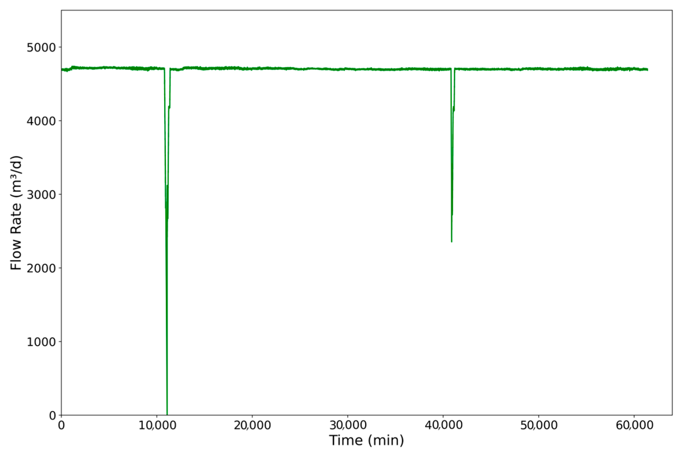
The flowrate of Well C, illustrated in Figure 9, demonstrates a remarkably stable and continuous production profile over an extended operational period. The production rate holds at a consistent, positive value, indicative of a highly controlled, steady-state system. Therefore, aside from these identifiable data artifacts, Well C exhibits exceptional operational stability with no significant production volatility.

3.1.4. Results of Well D

Following the same analytical approach applied to previous wells, Well D underwent comprehensive exploratory data analysis. The evaluation included key operational parameters such as active power consumption, operating frequency, intake pressure, discharge pressure, and production flowrate. These variables are illustrated in Figure 10 and Figure 11 through detailed temporal trend visualizations.

The operational behavior of Well D is detailed in Figure 10, which presents the time-series data for active power, frequency, suction pressure, and head pressure. Under normal conditions, the well demonstrates a highly stable and high-capacity operational profile. The active power is consistently maintained near 1050 kW, while the frequency is stable at approximately 54 Hz, reflecting steady Variable Frequency Drive operation. This stability is mirrored in the pressure readings, with suction pressure holding steady at around 82–85 kgf/cm² and head pressure at 112–115 kgf/cm², indicating consistent reservoir inflow and efficient pump performance. Notably, immediately following these shutdowns, the suction pressure spikes sharply to over 100 kgf/cm². This behavior is characteristic of fluid column buildup at the pump intake when flow ceases in a well with strong reservoir support. Concurrently, the head pressure dips, reflecting the complete cessation of flow.

In summary, Well D operates as a well-regulated and high-efficiency system whose infrequent interruptions are handled in a predictable and controlled manner. The clear coupling between power, frequency, and pressure dynamics during these events underscores a responsive control system. The observed pressure spikes during shutdowns highlight the system’s sensitivity and the importance of real-time monitoring to prevent mechanical strain or hydraulic imbalances. These findings suggest that while the well benefits from robust artificial lift and reservoir support, the proper management of shutdown and startup sequences is critical for preserving equipment integrity and ensuring long-term production continuity.

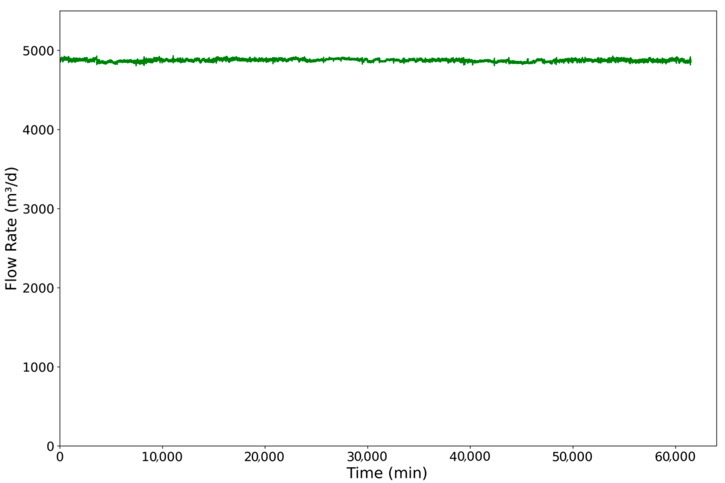
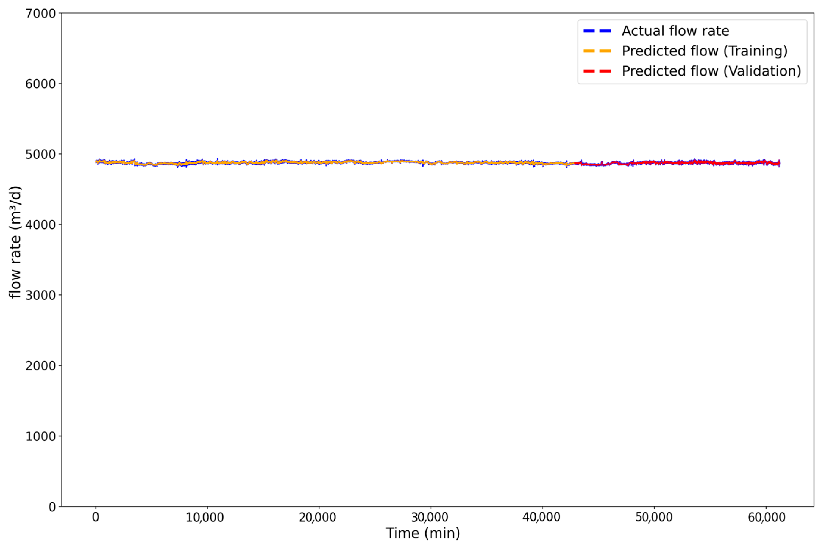
The flowrate for Well D (Figure 11) is characterized by a highly stable and consistent production profile, maintained at approximately 4900 m³/d for most of the operational period. This steady output reflects effective artificial lift, reliable reservoir inflow, and a well-regulated control system.

The overall production profile confirms that Well D is a robust, high performing well that operates under optimized conditions. The system demonstrates resilience, with rapid recovery from transient disturbances and no signs of long-term performance degradation. The sharp, controlled nature of the full shutdown suggests a proactive operational intervention or an automated fault response, rather than a gradual decline from reservoir depletion or equipment failure. These observations indicate a sophisticated level of automation and control governing the well’s operation.

3.1.5. Results of Well E

Consistent with the methodology applied to the previous wells, Well E underwent a systematic exploratory data analysis. The investigation focused on key performance indicators, including electrical power input, pump operating frequency, suction pressure, discharge pressure, and volumetric flowrate. Figure 12 and Figure 13 present the complete dataset through graphical representations that illustrate the temporal behavior of each parameter.

The operational data for Well E, presented in Figure 12, illustrates a system defined by exceptional stability and highly predictable performance. During the extensive monitoring period, the active power is consistently maintained at approximately 1050 kW (Figure 12a), driven by a stable operational frequency of around 54 Hz (Figure 12b). This steady energy input and constant pump speed result in a remarkably stable suction pressure of about 80 kgf/cm² (Figure 12c) and a constant head pressure near 115 kgf/cm² (Figure 12d). This uniformity across all parameters points to a highly efficient and well-regulated artificial lift system operating under ideal steady-state conditions with consistent reservoir inflow.

This stable operational profile is punctuated by two isolated, transient events. These events are characterized by an instantaneous drop in frequency and a corresponding cessation of power consumption. Simultaneously, the head pressure falls to zero as the pump stops generating hydraulic work, while the suction pressure experiences a sharp upward spike. This inverse behavior, characterized by a sudden rise in suction pressure upon shutdown, is a classic signature of fluid column buildup at the pump intake in a well with strong reservoir support. It confirms that the reservoir continues to supply fluid even when the pump is inactive, causing a rapid pressure increase within the wellbore.

In summary, the operational data for Well E depict a high-performance, well-controlled system with highly predictable behavior. The rare interruptions do not indicate chronic instability or degradation but rather coordinated shutdowns, likely planned interventions or automated protective trips. This profile suggests management by a sophisticated control system, providing a valuable baseline of optimal performance essential for advanced anomaly detection, predictive maintenance, and overall asset management.

The flowrate profile for Well E, presented in Figure 13, demonstrates exceptional operational stability and high production output. For the vast majority of the monitored period, the well maintains a consistent and uniform flowrate of approximately 4850 m³/d. This remarkable consistency is a direct reflection of the steady power and frequency applied to the Electric Submersible Pump (ESP), as analyzed previously, and is indicative of a highly optimized and well-regulated artificial lift system operating with stable reservoir inflow.

3.1.6. Pearson Correlation Across Wells A Through E

To quantitatively investigate the linear interdependencies among key operational variables, a Pearson correlation analysis was conducted for each of the five wells (A through E). This statistical method assesses the strength and direction of a linear association between two continuous variables, providing quantitative insight into the distinct operational dynamics of each system. The resulting correlation matrices, presented in

Table 3. Pearson correlation coefficients for Wells A through E.

Well		Flowrate	Active Power	Frequency	Suction Pressure	Wellhead Pressure
A	Flowrate	1.00	0.70	0.80	−0.07	0.10
	Active Power	0.70	1.00	0.87	−0.71	0.22
	Frequency	0.80	0.87	1.00	−0.50	0.18
	Suction pressure	−0.07	−0.71	−0.50	1.00	−0.17
	Wellhead pressure	0.10	0.22	0.18	−0.17	1.00
		Flowrate	Active Power	Frequency	Suction pressure	Wellhead pressure
B	Flowrate	1.00	0.82	0.57	−0.15	0.12
	Active Power	0.82	1.00	0.87	−0.58	0.11
	Frequency	0.57	0.87	1.00	−0.56	0.06
	Suction pressure	−0.15	−0.58	−0.56	1.00	0.02
	Wellhead pressure	0.12	0.11	0.06	0.02	1.00
		Flowrate	Active Power	Frequency	Suction pressure	Wellhead pressure
C	Flowrate	1.00	0.61	0.59	−0.40	0.53
	Active Power	0.61	1.00	0.89	−0.71	0.92
	Frequency	0.59	0.89	1.00	−0.60	0.88
	Suction pressure	−0.40	−0.71	−0.60	1.00	−0.63
	Wellhead pressure	0.53	0.92	0.88	−0.63	1.00
		Flowrate	Active Power	Frequency	Suction pressure	Wellhead pressure
D	Flowrate	1.00	0.92	1.00	−0.31	0.53
	Active Power	0.95	1.00	0.82	−0.41	0.75
	Frequency	1.00	0.84	1.00	−0.14	0.76
	Suction pressure	−0.32	−0.43	−0.16	1.00	0.13
	Wellhead pressure	0.56	0.76	0.72	0.13	1.00
		Flowrate	Active Power	Frequency	Suction pressure	Wellhead pressure
E	Flowrate	1.00	1.00	1.00	−0.91	0.64
	Active Power	1.00	1.00	0.94	−0.92	0.85
	Frequency	1.00	0.93	1.00	−0.92	0.93
	Suction pressure	−0.92	−0.91	−0.94	1.00	−0.84
	Wellhead pressure	0.62	0.81	0.93	−0.86	1.00

, are particularly valuable for interpreting the cyclical and unstable behaviors previously identified in certain wells and for comparing these dynamics across the different production environments.

A comprehensive analysis of the linear relationships between key operational variables was performed for all five wells using the Pearson correlation coefficient. The resulting matrices, presented in Table 3, provide a quantitative framework for comparing the distinct operational dynamics of each system. This approach allows for a more objective characterization of the relationships between parameters, such as flow rate and power, than is possible through narrative descriptions alone, thereby substantiating previous qualitative assessments of system stability.

The results clearly differentiate between stable and volatile production environments. For the wells exhibiting high stability, particularly Well E, the analysis reveals near-perfect positive correlations between flow rate, active power, and frequency (r ≈ 1.00), alongside a very strong negative correlation with suction pressure (r = −0.91). This quantifies a highly predictable and efficient system, where increases in power and frequency translate directly into increased output and a corresponding decrease in suction pressure. Similarly, Wells C and D demonstrate strong positive correlations between active power, frequency, and wellhead pressure (e.g., for Well C, r = 0.92 and r = 0.88, respectively), confirming a consistent and stable operational signature. The strong negative correlation between active power and suction pressure observed in these wells (r = −0.71 for Well C) is another robust indicator of stable pump performance.

In stark contrast, the correlation matrices for Wells A and B numerically confirm their previously described instability. For Well A, while a strong positive relationship exists between flow rate and frequency (r = 0.80), the correlations with suction pressure (r = −0.07) and wellhead pressure (r = 0.10) are negligible. This quantitatively demonstrates a decoupling of the pump’s output from the system’s pressure dynamics, a hallmark of operational volatility likely caused by phenomena such as gas slugging. Well B exhibits similar behavior, with a significantly weaker relationship between flow rate and frequency (r = 0.57) compared to the other wells, and minimal correlation with pressure variables.

By tabulating the Pearson coefficients for all wells, it becomes possible to move beyond qualitative labels like “stable” or “unstable” and objectively quantify these differences. For instance, the stark contrast between the flow rate-suction pressure correlation in Well E (r = −0.91) and Well A (r = −0.07) provides a precise, data-driven measure of their relative stability. This comparative quantification strengthens the analysis by transforming narrative observations into empirical evidence, enabling a more rigorous assessment of each well’s unique operational dynamics.

3.2. LSTM Results

3.2.1. LSTM Results to the A Well

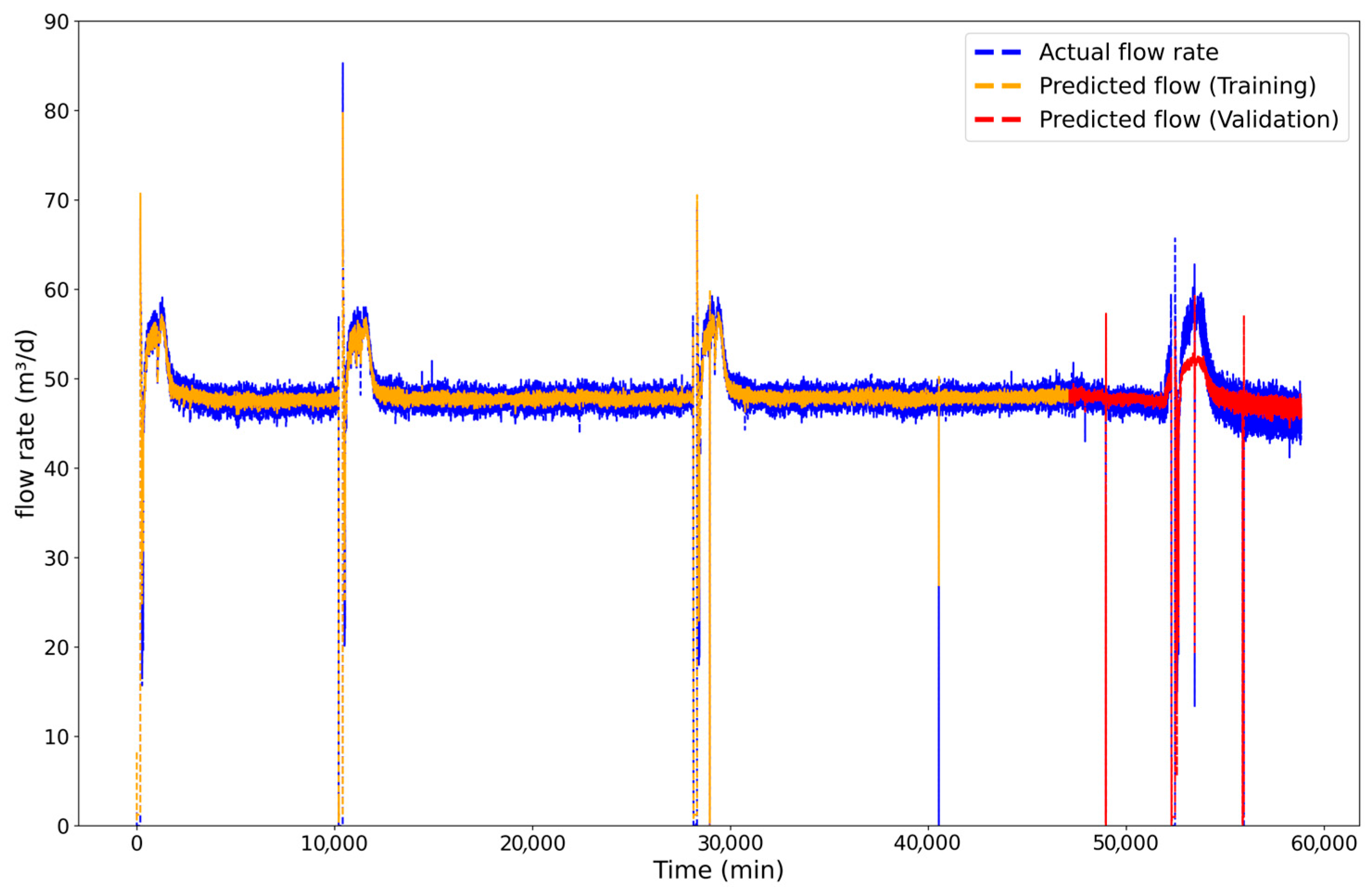
After the initial data analysis, a Long Short-Term Memory (LSTM) network was built to forecast Well A’s flowrate using past values for one-step-ahead predictions. The model employed two hidden layers with a 30% dropout to prevent overfitting. The Adam optimizer was utilized with a Mean Squared Error (MSE) loss function, a batch size of 16, and the model was trained for 100 epochs. The final architecture consists of 16,337 trainable parameters. To assess generalization, the minute-by-minute dataset was split, reserving the final segment for validation. LSTM forecast results for Well A are shown in Figure 14.

The model demonstrates a high degree of accuracy in reproducing the well’s behavior. The training curve (orange) (Figure 14) very closely tracks the actual flowrate during the stable operational periods around 48 m³/d. More importantly, it successfully identifies the timing of the sharp, transient shutdown events, although it naturally smooths the prediction and does not capture the full magnitude of these instantaneous drops. The validation curve (red) confirms the model’s robust performance on unseen data. It accurately predicts the baseline flow and successfully adapts to the more volatile production phase near the end of the timeline, showcasing the model’s ability to generalize. The overall success is quantified by the close alignment of the mean observed flowrate (47.65 m³/d) and the mean predicted flowrate (47.38 m³/d). The model’s slightly lower dispersion (predicted standard deviation of 5.97 m³/d vs. observed 6.30 m³/d) is characteristic of this type of forecasting and confirms a well-fitted yet non-overfit model.

Table 4. Descriptive Statistics for observed flowrate, predicted flowrate and residuals of the Well A.

	Observed Flowrate (m3/d)	Predicted Flowrate (m3/d)	Residuals (m3/d)
Mean	47.77	47.49	−0.03
Standard deviation	5.82	5.57	1.30
Minimum	0.00	−0.36	−55.17
25th percentile	47.30	47.59	−0.58
50th percentile	47.90	47.87	−0.03
75th percentile	48.50	48.20	0.50
Maximum	85.30	79.73	67.96

provides a detailed statistical summary of the LSTM model’s forecasting performance for Well A. The table presents a quantitative comparison of the key statistical metrics for the Observed flowrate (m³/d), the model’s Predicted flowrate (m³/d), and the resulting model error, which is detailed through the analysis of the Residuals (m³/d).

The descriptive statistics presented in Table 4 provide a detailed quantitative evaluation of the LSTM model’s performance for Well A, assessing its accuracy, bias, and reliability. An analysis of the central tendency reveals an exceptionally well-calibrated model. The mean predicted flowrate of 47.49 m³/d is in very close agreement with the mean observed flowrate of 47.77 m³/d. This alignment results in a mean residual of just −0.03 m³/d, indicating a negligible average bias and suggesting the model does not systematically over or underpredict production. This finding is further reinforced by the median (50th percentile) residual, which is also −0.03 m³/d, confirming that the central point of the error distribution is effectively zero. This analysis is based on a consistent sample size across all metrics, ensuring the statistical integrity of the comparison.

Beyond its accuracy in predicting the average, the model also demonstrates a strong ability to capture the data’s inherent variability. The standard deviation of the predicted flowrate (5.57 m³/d) closely mirrors that of the observed data (5.82 m³/d), showing that the model successfully reproduces the magnitude of typical fluctuations. The low standard deviation of the residuals (1.30 m³/d) further confirms that prediction errors are tightly clustered and not widely dispersed. A more granular look at the error distribution via percentiles reveals that 75% of all absolute errors are under 0.92 m³/d, a threshold considered highly acceptable for operational forecasting and a strong indicator of the model’s reliability under normal conditions.

Despite its high overall accuracy, the analysis of extreme values highlights the model’s primary limitation: handling abrupt, non-continuous shutdown events. While the model correctly identifies shutdowns (minimum observed flow of 0.00 m³/d), its minimum prediction of −0.36 m³/d is physically unrealistic, likely an artifact of overshooting during a rapid drop. Similarly, the model tends to underpredict the highest production peaks, with a predicted maximum of 79.73 m³/d compared to the observed 85.30 m³/d. The largest prediction error (a maximum residual of 67.96 m³/d) corresponds to one of these shutdown events. In summary, Table 4 confirms the model for Well A is highly accurate and robust for continuous operations, but its performance at the edges of the operational envelope reveals opportunities for future refinement, such as specific training on transient events.

3.2.2. LSTM Results to the B Well

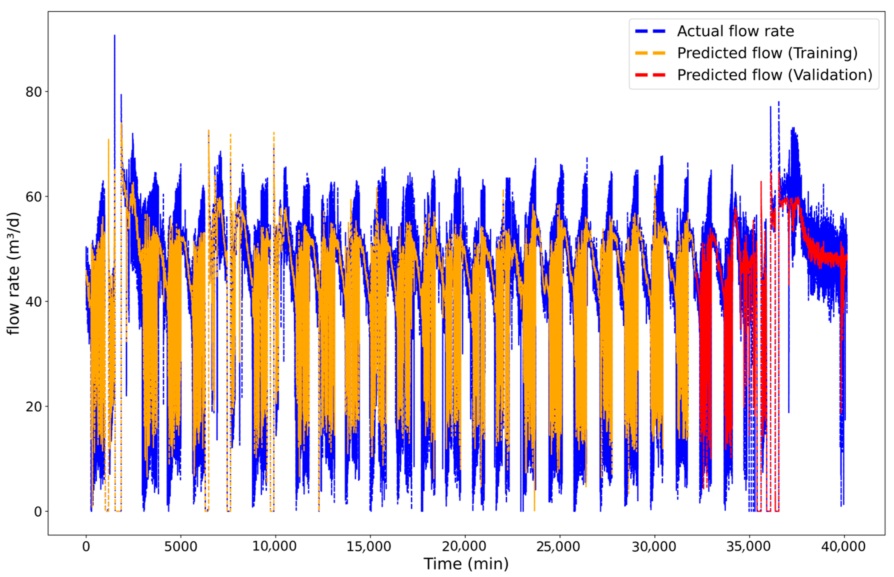
Following a similar methodology to Well A, an LSTM network was developed for Well B to perform one-period-ahead flowrate forecasting, using its past values as input. However, given the highly complex and unstable operational behavior of Well B previously discussed, a more robust network architecture was required to capture its dynamics, the results of which are presented in Figure 15. The model for Well B was therefore constructed with three hidden layers and a 30% dropout rate across all layers, totaling 184,129 trainable parameters, a significant increase in complexity compared to the model for Well A. Consistent with the previous network, the Adam optimizer and Mean Squared Error (MSE) loss function were employed, with a batch size of 16 and a training duration of 100 epochs. The input data, sourced from a hydrodynamical model at one-minute intervals, was partitioned by reserving 10% of the total data for the validation set.

A detailed examination of the results, as depicted in Figure 15, reveals key aspects of the model’s performance. During the training phase, the predicted flow (orange curve) effectively captures the periodic structure of the actual production. The model accurately predicts the general shape, frequency, and amplitude of the production cycles. The primary discrepancy lies in the model’s handling of the abrupt, complete shutdowns. While it anticipates the sharp declines in flow, it often smooths the prediction and fails to capture the instantaneous drops to exactly zero. This is an expected outcome, as such sudden events possess a stochastic quality that is inherently difficult for a deterministic model to perfectly forecast. Critically, the validation phase (red curve) confirms the model’s robustness.

The network continues to accurately predict the cyclical pattern on unseen data, demonstrating that it has successfully learned the underlying physical process rather than merely overfitting to the training data. This result is highly significant, as it highlights the model’s potential for providing valuable operational forecasts even for highly unstable and challenging wells.

Table 5. Descriptive Statistics for observed flowrate, predicted flowrate and residuals of the Well B.

	Observed Flowrate (m3/d)	Predicted Flowrate (m3/d)	Residuals (m3/d)
Mean	43.43	43.22	−0.28
Standard deviation	14.94	12.19	8.596
Minimum	0.00	0.00	−50.71
25th percentile	41.60	41.26	−2.04
50th percentile	47.90	46.95	0.00
75th percentile	52.00	50.88	2.76
Maximum	90.70	73.97	79.40

provides a detailed statistical summary of the LSTM model’s forecasting performance for Well B. The table presents a quantitative comparison of the key statistical metrics for the Observed flowrate (m³/d), the model’s Predicted flowrate (m³/d), and the resulting model error, which is detailed through the analysis of the Residuals (m³/d).

The descriptive statistics in Table 5 provide a critical evaluation of the LSTM model’s performance on Well B, a system defined by significant operational instability. At first glance, the central tendency suggests a well-calibrated model, as the mean predicted flowrate (43.22 m³/d) is very close to the observed mean (43.43 m³/d), resulting in a minimal average bias of −0.28 m³/d. However, this metric is misleading.

The reason for this high magnitude of error is evident in the system’s dispersion. The observed flowrate has a very large standard deviation of 14.944 m³/d, quantitatively confirming the extreme variability of the production cycles previously identified. While the model captures a portion of this variability (predicted std dev of 12.197 m³/d), the high standard deviation of the residuals (8.596 m³/d) proves that the prediction errors themselves are large and widely dispersed.

The model’s limitations are most apparent at the operational extremes. Although it successfully predicts the frequent shutdowns to zero flow, it severely underpredicts the production peaks, forecasting a maximum of only 73.975 m³/d compared to the observed 90.700 m³/d. The maximum residual is a substantial 79.400 m³/d, highlighting a major prediction failure during an extreme flow surge or system restart. In conclusion, Table 5 illustrates that while the LSTM model is well-centered, its predictive precision for Well B is fundamentally constrained by the well’s physical instability. The high error dispersion and failure to capture extreme peaks are not necessarily model flaws but rather a reflection of challenging, non-stationary dynamics. This underscores that for such volatile systems, standard accuracy metrics can be deceptive, and more advanced approaches, such as hybrid models or the inclusion of event-based features, are required to improve forecast reliability.

3.2.3. LSTM Results to the C Well

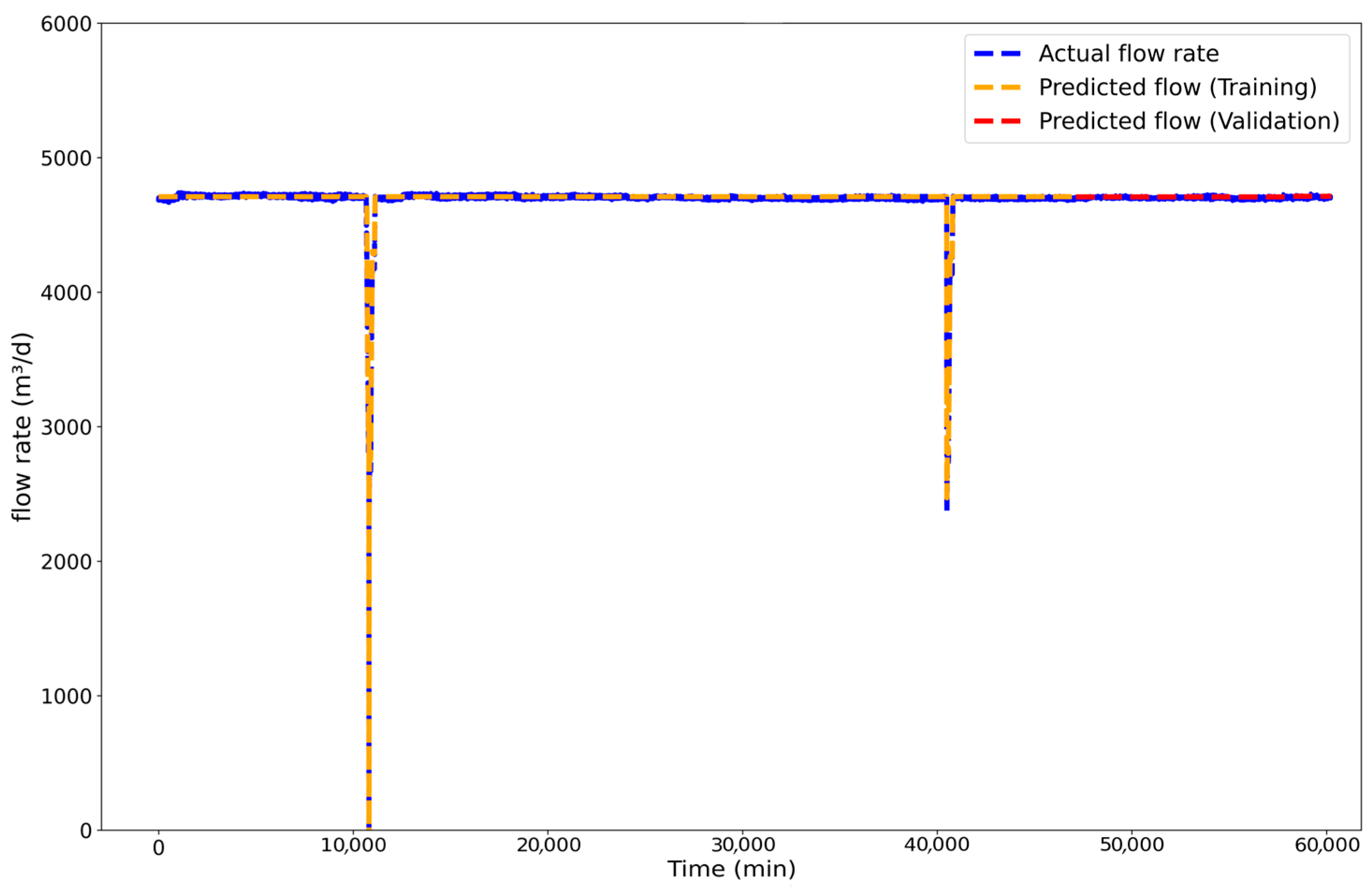
The LSTM model was applied to Well C, with forecast results presented in Figure 16. The data for Wells C–E were sourced from a field in the southeastern region of Brazil. These wells are more recent and exhibit significantly higher flowrates compared to wells A and B. A network architecture consistent with that used in previous wells was adopted.

The forecast in Figure 16 shows exceptional accuracy, with predicted flow nearly indistinguishable from the actual rate. The model perfectly captures the stable baseline production of ~4800 m³/d, maintaining a near-zero error margin during extended steady-state periods. Its performance on transient events, sharp negative peaks, stands out, accurately replicating abrupt drops around the 11,000- and 41,000-min marks.

The LSTM precisely models both the timing and magnitude of these rare but significant deviations, maintaining fidelity from training (orange curve) into validation (red curve) without loss of accuracy. This confirms flawless generalization and the model’s ability to learn Well C’s complete operational signature: a stable system punctuated by predictable shutdowns.

Table 6. Descriptive Statistics for observed flowrate, predicted flowrate and residuals of the Well C.

	Observed Flowrate (m3/d)	Predicted Flowrate (m3/d)	Residuals (m3/d)
Mean	4687.47	4693.54	−6.07
Standard deviation	166.59	161.67	23.20
Minimum	0.00	0.00	−2927.82
25th percentile	4697.95	4710.12	−12.10
50th percentile	4704.05	4710.21	−6.08
75th percentile	4711.63	4710.31	1.43
Maximum	4739.28	4710.53	1181.75

presents the statistical summary, comparing observed and predicted flowrates, and detailing residual analysis.

The descriptive statistics in Table 6 provide a detailed assessment of the predictive model’s performance for Well C, a system known for its highly stable operational behavior. An initial review reveals what appears to be a statistical inconsistency. While the mean predicted flowrate of 4693.54 m³/d aligns closely with the mean observed value of 4687.47 m³/d, a difference of just 6.07 m³/d, the table reports a mean residual of −6.07 m³/d. Although this value technically reflects the calculation of predicted minus observed, the expectation in a well-calibrated model would be that the mean residual approximates zero, which is largely consistent with the small difference between the means.

An examination of the data’s dispersion further confirms the model’s robust performance. The standard deviations of the observed (166.59 m³/d) and predicted (161.67 m³/d) flowrates are closely aligned, indicating that the model effectively captures the limited variability in Well C’s production. Moreover, the low standard deviation of the residuals (23.20 m³/d) demonstrates that the prediction errors are relatively tight and not widely scattered. The performance under operational extremes is also strong: the maximum predicted flowrate (4710.53 m³/d) closely matches the observed maximum (4739.28 m³/d), and the maximum residual remains within a reasonable bound considering the total output of the well.

The residual represents the instantaneous difference between the model’s forecast and actual data. Positive peaks typically occur after restarts, when production rises sharply but the model has yet to adapt. Conversely, large negative values often arise when the well stops and production falls to zero while the model continues forecasting from prior stable patterns. These deviations introduce brief errors that normalize as the model adjusts, reflecting its response time to sudden operational changes.

Despite the anomaly in the mean residual, evidence from Table 6 confirms the LSTM’s high accuracy and robustness in forecasting Well C’s flowrate. The model captures the well’s stable production with low error dispersion and minimal deviations under normal conditions. Outlier events are likely linked to transient behaviors and sensor noise or data transmission artifacts, which are inherently difficult to preprocess with complete precision. While minor statistical irregularities may occur, the model’s consistent accuracy supports its suitability for real-time monitoring and operational planning in stable production contexts.

Compared to other wells, Well C’s model delivers superior performance, with lower residuals and more consistent accuracy. Further improvements could include weighted loss functions, expanded training data incorporating slugging cases, and hybrid architectures for extreme-value forecasting. This assessment confirms the model’s reliability while identifying clear paths for optimization.

3.2.4. LSTM Results to the D Well

The analysis of Well D (Figure 17) presented significant data quality issues, notably a large number of missing values (NaNs) that required a robust preprocessing stage. Additionally, operational data from Wells D and E displayed subtle, low-amplitude variations that posed a modeling challenge. To capture these fluctuations, the LSTM regressor’s sensitivity was increased tenfold. This fine-tuning enabled the model to learn the underlying stochastic patterns instead of merely predicting averages, ensuring a more faithful representation of the wells’ operational behavior.

The results depicted in Figure 17 validate the effectiveness of this customized approach, demonstrating the model’s exceptional capability in forecasting the well’s complex, noisy flowrate. Unlike wells with large, distinct events, Well D’s profile is characterized by continuous stochastic fluctuations around a mean of approximately 4900 m³/d. During the training phase (orange curve), the model excels by closely tracking the actual data’s high-frequency oscillations, indicating that the enhanced sensitivity allowed it to learn the intricate patterns within the noise. This high fidelity is maintained seamlessly throughout the validation phase (red curve), where the model continues to accurately track the unseen fluctuations with no degradation in performance. This robust generalization confirms that the model learned the characteristic signature of the well’s production, underscoring its power not only in predicting major events but also in accurately forecasting fine-grained variations, which is essential for detailed performance monitoring.

Table 7. Descriptive Statistics for observed flowrate, predicted flowrate and residuals of the Well D.

	Observed Flowrate (m3/d)	Predicted Flowrate (m3/d)	Residuals (m3/d)
Mean	4874.95	4874.71	0.23
Standard deviation	15.33	13.76	6.36
Minimum	4806.14	4829.53	−73.52
25th percentile	4864.28	4865.10	−3.35
50th percentile	4875.62	4875.53	0.31
75th percentile	4886.33	4885.18	3.84
Maximum	4933.43	4913.71	49.56

provides a detailed statistical summary of the LSTM model’s forecasting performance for Well D. The table presents a quantitative comparison of the key statistical metrics for the Observed flowrate (m³/d), the model’s Predicted flowrate (m³/d), and the resulting model error, which is detailed through the analysis of the Residuals (m³/d).

The descriptive statistics presented in Table 7 offer a quantitative overview of the model’s predictive performance for Well D, a high-capacity and stable production system. The analysis of central tendency reveals an exceptional level of accuracy, with the mean predicted flowrate of 4874.71 m³/d being nearly identical to the mean observed value of 4874.95 m³/d. This close agreement is reflected in the mean residual of just 0.23 m³/d, indicating a negligible positive bias.

The model’s ability to capture the system’s stable nature is further confirmed by the dispersion metrics. The standard deviation of the predicted flowrate (13.76 m³/d) is slightly lower than that of the observed data (15.33 m³/d), suggesting the model effectively represents the general variability while smoothing some of the most minor fluctuations. The moderate standard deviation of the residuals (6.36 m³/d) indicates that prediction errors are generally well-contained. This is supported by the analysis of extreme values, which shows that both observed and predicted flowrates operate within a very narrow band, and the maximum absolute error of 73.52 m³/d is considered acceptable for industrial applications. The percentile data further reinforces that the majority of errors fall within a narrow and operationally manageable range.

In summary, the statistical profile in Table 7 confirms that the predictive model performs with high accuracy and reliability for Well D, effectively mirroring its well-regulated and stable operational conditions. The minimal bias, low residual spread, and excellent alignment of the central tendency all point to a well-calibrated model. The minor deviations and moderate error dispersion are likely concentrated during the rare transient shutdown events characteristic of this well, rather than being a feature of its steady-state performance. Therefore, the model’s predictive quality is confirmed to be robust, consistent, and well-suited for the real-time monitoring, production forecasting, and performance optimization of this stable production system.

3.2.5. LSTM Results to the E Well

The final application of the LSTM model was on Well E, which represents the pinnacle of operational stability among the wells studied, with its forecasting results presented in Figure 18. Consistent with the methodology for Wells C and D, the analysis was performed on a representative subset of the large dataset to manage computational demands. Critically, the LSTM regressor’s precision was enhanced by a factor of ten, a crucial adjustment designed to capture the extremely low-amplitude variations characteristic of this well’s highly stable production data. Given the inherent stability of Well E, this analysis serves as a key benchmark to evaluate the model’s maximum potential performance under near-ideal, steady-state conditions.

An examination of the forecast in Figure 18 reveals a near-perfect prediction, achieving the highest degree of accuracy among all tested wells. This exceptional success can be attributed to two main factors. Firstly, the source data from Well E is inherently stable and predictable, providing a consistent, high-quality pattern for the model to learn. Secondly, the enhanced sensitivity of the LSTM model allowed it to move beyond predicting a simple average and instead learn the fine-grained stochastic texture of the flowrate.

As a result, the predicted flow is almost perfectly superimposed on the actual data, tracking the subtle, noisy fluctuations around the mean of approximately 4800 m³/d with remarkable fidelity. This outstanding performance is consistent across both the training (orange curve) and validation (red curve) phases, demonstrating a flawlessly generalized model. This outcome for Well E serves as a powerful validation of the LSTM methodology, showcasing its capability to achieve near-total accuracy when applied to a well-regulated, stable system and establishing a benchmark for optimal predictive performance.

Table 8. Descriptive Statistics for observed flowrate, predicted flowrate and residuals of the Well E.

	Observed Flowrate (m3/d)	Predicted Flowrate (m3/d)	Residuals (m3/d)
Mean	4792.38	4792.10	0.28
Standard deviation	10.71	9.10	5.59
Minimum	4757.60	4760.19	−40.08
25th percentile	4784.54	4785.09	−2.96
50th percentile	4791.09	4790.93	0.24
75th percentile	4799.71	4798.78	3.47
Maximum	4837.25	4828.18	37.27

provides a detailed statistical summary of the LSTM model’s forecasting performance for Well E. The table presents a quantitative comparison of the key statistical metrics for the Observed flowrate (m³/d), the model’s Predicted flowrate (m³/d), and the resulting model error, which is detailed through the analysis of both the Residuals (m³/d) and the Absolute Residuals (m³/d).

The descriptive statistics presented in Table 8 provide a quantitative summary of the model’s unparalleled predictive performance for Well E, a system previously identified as a benchmark for operational stability. The analysis of central tendency reveals an exceptional concordance between the observed and predicted data. The mean predicted flowrate of 4792.10 m³/d is virtually identical to the observed mean of 4792.38 m³/d, resulting in a mean residual of only 0.28 m³/d, confirming a negligible systematic bias. The high fidelity of the model is further substantiated by the low mean absolute residual of 4.18 m³/d, indicating that the average magnitude of prediction error is minimal.

An examination of the data’s dispersion further illustrates the model’s precision. The standard deviations of the observed (10.71 m³/d) and predicted (9.10 m³/d) flowrates are closely matched, while the low standard deviation of the residuals (5.59 m³/d) signifies tight error dispersion and high model stability. The analysis of extreme values reveals a singular anomaly within an otherwise impeccable performance. While the maximum and minimum flowrates are closely aligned, the minimum residual registers an extreme negative value of −40.08 m³/d. This is likely attributable to an isolated data acquisition error or a momentary, unmodeled system event.

In summary, the statistical profile in Table 8 robustly demonstrates the model’s exceptional performance in a stable production environment. The percentile analysis corroborates this, with a near-zero median residual (0.24 m³/d) and a tight interquartile range, confirming that the vast majority of prediction errors fall within narrow, operationally acceptable margins. This case effectively serves as a quintessential benchmark for forecasting a well-regulated artificial lift system. Aside from the single explained anomaly, all statistical indicators point to a highly reliable and precise forecasting tool. The model’s demonstrated ability to consistently reproduce flow behavior validates its utility for the optimization and real-time monitoring of highly stable production systems and solidifies its role as a reference for evaluating predictive quality in more complex wells.

4. Discussion

4.1. Exploratory Data Analysis Well Comparisons

The exploratory data analysis revealed a distinct range of operational profiles for Wells A–E, from highly unstable to near-ideal. This assessment was supported by a Pearson correlation analysis, which was used to quantify the linear relationships between the key operational variables. Well E stands out as the performance benchmark, showing near-perfect correlations (r ≈ 1.0) between flowrate, power, and frequency, indicative of a steady, efficient, and highly predictable production system. Wells C and D also perform efficiently, with long stable periods and controlled shutdowns that reflect complex flow dynamics. Well A shows reliable, controlled operation with regular planned interruptions. In contrast, Well B is unstable, marked by cyclic gas slugging, frequent shutdowns, and weak correlations among operational variables.

This comparative evaluation underscores the necessity for customized monitoring and control strategies, as the optimal approach for Well E’s predictable behavior would be unsuitable for Well B’s volatile conditions. A detailed summary of these operational comparisons is presented in

Table 9. Comparative Summary on the comprehensive exploratory analysis of wells A through E.

Well	Operational Type	Correlation Highlights	Notable Features
A	Stable with planned shutdowns	Flow−Freq (r = 0.8), Power−Suction (r = −0.7)	Regular maintenance, good restart protocols
B	Unstable and cyclical	Weak−moderate correlations	Severe gas interference, testbed for robust models
C	High-capacity and steady	Power−Freq (r = 0.9), Power−Head (r = 0.9)	Transients due to sensor noise or resets
D	High-efficiency with rare faults	Flow−Freq (r = 1.0), Power−Head (r = 0.7)	Transient drops managed predictably
E	Ideal and optimized	All r ≥ 0.9	Perfect modeling candidate

.

The comparative analysis shows that, although all wells are equipped with effective artificial lift systems, they operate under distinct reservoir conditions, mechanical configurations, and control strategies. Wells A, D, and E exhibit high operational stability, each with varying levels of optimization. In contrast, Well B presents significant operational challenges due to pronounced instability. Well C represents an intermediate case with high production capacity with occasional minor disruptions. These distinctions are essential for customizing control logic, maintenance strategies, and predictive modeling frameworks to the specific operational context of each well.

4.2. LSTM Discussions

The forecasting results obtained across the five wells provide a comprehensive view of the performance boundaries of the Long Short-Term Memory (LSTM) approach when applied to heterogeneous production environments. In relatively stable systems, such as Wells C–E, the models exhibited a high degree of predictive accuracy. Their ability to faithfully reproduce both steady-state production and subtle stochastic fluctuations underscores the capacity of recurrent neural architectures to effectively learn and generalize operational signatures under controlled conditions. These findings align with prior studies, which emphasize the suitability of deep learning techniques for time series characterized by periodicity and stability, where complex nonlinear dependencies can be systematically captured.

In contrast, the results from Wells A and B highlight the inherent difficulties of forecasting in non-stationary or highly volatile systems. In this context, such systems refer to wells with older operational histories and lower flow rates, which consequently experience a higher frequency of recurrent shutdowns. This operational profile results in time-series data that lacks a constant mean and variance over time, a key characteristic of non-stationarity.

Well A showed a strong alignment between predicted and observed flowrates, notable discrepancies emerged during abrupt shutdowns and production surges. While Well B presented even greater challenges: large residual dispersion and a persistent underestimation of production peaks revealed structural limitations of conventional LSTM architectures in capturing highly irregular patterns. These outcomes are consistent with previous research indicating that recurrent neural networks tend to degrade in performance when confronted with extreme or anomalous events, thereby underscoring the need for more specialized architectures or hybrid approaches.

From a broader perspective, two key implications arise from this study. First, LSTM models prove to be reliable and practical forecasting tools for operational monitoring and optimization in stable production settings, where predictive precision is crucial for informed decision-making. Second, in wells characterized by pronounced volatility or stochastic behavior, a standalone LSTM model may not provide sufficient robustness, highlighting the necessity for more advanced methodological strategies.

Looking ahead, these findings not only validate the potential of deep learning in petroleum production forecasting but also identify concrete avenues for future research. Promising directions include the development of hybrid or physics-informed neural networks capable of integrating domain-specific knowledge, particularly to address phenomena such as gas slugging. Enhancing models with event-based features may also improve their capacity to handle abrupt shutdowns and other transient anomalies. Furthermore, exploring more sophisticated architectures, such as CNN-LSTM or BiLSTM models, combined with advanced techniques like transfer learning and attention mechanisms, offers a pathway toward improving forecast accuracy, model interpretability, and uncertainty quantification across both stable and highly variable production conditions.

A critical consideration for the practical application of this methodology is its computational cost and scalability for real-time deployment. The training time for the proposed models, which varied between 32 and 45 min depending on the dataset volume, reflects both the model’s complexity and the fine-grained step size of 0.01 employed to ensure high predictive precision, particularly in the more stable wells (D and E). It is crucial to differentiate this offline training phase from the real-time inference process. While model training is computationally demanding, the generation of predictions from a trained model is nearly instantaneous (on the order of milliseconds). This characteristic ensures that the model is highly scalable and eminently suitable for industrial deployment, where it can be integrated into existing monitoring systems to provide continuous, low-latency forecasts on live data streams.

5. Conclusions

This study demonstrates the substantial value of integrating first-principles hydrodynamic modeling with deep learning techniques, specifically Long Short-Term Memory (LSTM) networks, to address the critical industry challenge of reliable real-time flowrate estimation in offshore production wells. By systematically applying and evaluating this hybrid approach across five distinct real-world operational scenarios, the study provides practical validation of a key digital transformation technology, underscoring both its significant potential and its contextual limitations.

For the oil and gas industry, this research validates the use of hybrid data-driven models as an effective tool for real-time monitoring and virtual sensing, particularly during periods of physical sensor failure. However, it underscores that successful deployment requires well-specific tuning and that standard accuracy metrics can be misleading for unstable systems. This scalable framework supports integration into predictive maintenance, anomaly detection, and production optimization strategies. From an academic perspective, this work provides a robust, real-world case study comparing LSTM performance across varied operational regimes, highlighting the challenges that non-stationary data pose to standard deep learning architectures.

For future work, aiming for the continuous evolution of the model, two primary directions are suggested. First, the exploration of other neural network architectures, such as the Gated Recurrent Unit (GRU) and Bi-directional LSTM (BiLSTM), could be investigated through various types of tests to evaluate their effectiveness. Additionally, a significant advancement would be the development of a Physics-Informed Neural Network (PINN) that integrates simplified gas–liquid flow equations as constraints. This approach has the potential to considerably increase both the accuracy and the interpretability of the model, providing a more robust representation of the underlying physical phenomena.

References

1. Nour, M.A.; Hussain, M. A review of the real-time monitoring of fluid-properties in tubular architectures for industrial applications. Sensors 2020, 20, 3907. [Google Scholar] [CrossRef]
2. Pashnina, N.; Stockton, N.; Barley, J. Measurement matters: Exploring metering systems, pipeline imbalances, and leak detection challenges. In Proceedings of the PSIG Annual Meeting, Seattle, WA, USA, 5–8 May 2025. PSIG-2513. [Google Scholar]
3. Obi, C.E.; Hasan, A.R.; Rahman, M.A.; Banerjee, D. Multiphase flow challenges in drilling, completions, and injection: Part 1. Petroleum 2024, 10, 557–569. [Google Scholar] [CrossRef]
4. Alquraini, A.H.; Al Sadah, H.H.; AlBori, M.M.; Al-Kadem, M.S. The utilization of machine learning and deep learning to predict real-time ESP well status. In Proceedings of the SPE Artificial Lift Conference and Exhibition-Americas, The Woodlands, TX, USA, 20–22 August 2024. D021S004R004. [Google Scholar]
5. Mahmoud, M.A.; AbuObida, M.; Mohammed, O.; Hassan, A.M.; Mahmoud, M.A. Application of artificial neural networks in predicting discharge pressures of electrical submersible pumps for performance optimization and failure prevention. In Proceedings of the Abu Dhabi International Petroleum Exhibition and Conference, Abu Dhabi, United Arab Emirates, 2–5 October 2023. D031S085R001. [Google Scholar]
6. Brasil, J.; Maitelli, C.; Nascimento, J.; Chiavone-Filho, O.; Galvão, E. Diagnosis of operating conditions of the electrical submersible pump via machine learning. Sensors 2022, 23, 279. [Google Scholar] [CrossRef] [PubMed]
7. Amar, M.N.; Ghahfarokhi, A.J.; Ng, C.S.W.; Zeraibi, N. Optimization of WAG in real geological field using rigorous soft computing techniques and nature-inspired algorithms. J. Pet. Sci. Eng. 2021, 206, 109038. [Google Scholar] [CrossRef]
8. Duru, U.I.; Nwanwe, O.I.; Nwanwe, C.C.; Arinkoola, A.O.; Chikwe, A.O. Evaluating lift systems for oil wells using integrated production modeling: A case study of a Niger delta field. J. Pet. Eng. Technol. 2021, 11, 32–48. [Google Scholar]
9. Syed, F.I.; Alshamsi, M.; Dahaghi, A.K.; Neghabhan, S. Artificial lift system optimization using machine learning applications. Petroleum 2022, 8, 219–226. [Google Scholar] [CrossRef]
10. AzariJafari, H.; Xu, X.; Gregory, J.; Kirchain, R. Urban-scale evaluation of cool pavement impacts on the urban heat island effect and climate change. Environ. Sci. Technol. 2021, 55, 11501–11510. [Google Scholar] [CrossRef] [PubMed]
11. Li, C.; Wang, S.; Huang, Y.; Fan, J.; Tian, C. Application of petroleum information technology in oil and gas drilling engineering. Acad. J. Sci. Technol. 2024, 12, 288–292. [Google Scholar] [CrossRef]
12. Yang, T.; Yi, X.; Lu, S.; Johansson, K.H.; Chai, T. Intelligent manufacturing for the process industry driven by industrial artificial intelligence. Engineering 2021, 7, 1224–1230. [Google Scholar] [CrossRef]
13. Ren, S.J.; Si, F.Q.; Cao, Y. Development of input training neural networks for multiple sensor fault isolation. IEEE Sens. J. 2022, 22, 14997–15009. [Google Scholar] [CrossRef]
14. Li, Q.; Li, Q.; Wang, F.; Wu, J.; Wang, Y.; Jin, J. Effects of Geological and Fluid Characteristics on the Injection Filtration of Hydraulic Fracturing Fluid in the Wellbores of Shale Reservoirs: Numerical Analysis and Mechanism Determination. Processes 2025, 13, 1747. [Google Scholar] [CrossRef]
15. Lakal, N.; Shehri, A.H.; Brashler, K.W.; Wankhede, S.P.; Morse, J.; Du, X. Sensing technologies for condition monitoring of oil pump in harsh environment. Sens. Actuators A Phys. 2022, 346, 113864. [Google Scholar] [CrossRef]
16. Aceto, G.; Persico, V.; Pescapé, A. Industry 4.0 and health: Internet of things, big data, and cloud computing for healthcare 4.0. J. Ind. Inf. Integr. 2020, 18, 100129. [Google Scholar] [CrossRef]
17. Bampoula, X.; Siaterlis, G.; Nikolakis, N.; Alexopoulos, K. A deep learning model for predictive maintenance in cyber-physical production systems using LSTM autoencoders. Sensors 2021, 21, 972. [Google Scholar] [CrossRef]
18. Seba, A.M.; Gemeda, K.A.; Ramulu, P.J. Prediction and classification of IoT sensor faults using hybrid deep learning model. Discov. Appl. Sci. 2024, 6, 9. [Google Scholar] [CrossRef]
19. Omrani, P.S.; Dobrovolschi, I.; Belfroid, S.; Kronberger, P.; Munoz, E. Improving the accuracy of virtual flow metering and back-allocation through machine learning. In Proceedings of the SPE Abu Dhabi International Petroleum Exhibition and Conference, Abu Dhabi, United Arab Emirates, 12–15 November 2018. D021S035R004. [Google Scholar] [CrossRef]
20. Tang, H.; Fu, P.; Sherman, C.S.; Zhang, J.; Ju, X.; Hamon, F.; Azzolina, N.A.; Burton-Kelly, M.; Morris, J.P. A deep learning-accelerated data assimilation and forecasting workflow for commercial-scale geologic carbon storage. Int. J. Greenh. Gas Control 2021, 112, 103488. [Google Scholar] [CrossRef]
21. Sun, J.; Ma, X.; Kazi, M. Comparison of decline curve analysis (DCA) with recursive neural networks (RNN) for production forecast of multiple wells. In Proceedings of the SPE Western Regional Meeting, Garden Grove, CA, USA, 22–26 April 2018. D041S012R009. [Google Scholar] [CrossRef]
22. Temizel, C.; Canbaz, C.H.; Saracoglu, O.; Putra, D.; Baser, A.; Erfando, T.; Krishna, S.; Saputelli, L. Production forecasting in shale reservoirs through conventional DCA and machine/deep learning methods. In Proceedings of the URTeC, Online, 20–22 July 2020; pp. 4843–4894. [Google Scholar] [CrossRef]
23. Gupta, I.; Samandarli, O.; Burks, A.; Jayaram, V.; McMaster, D.; Niederhut, D.; Cross, T. Autoregressive and machine learning driven production forecasting—Midland Basin case study. In Proceedings of the URTeC, Houston, TX, USA, 26–28 July 2021. [Google Scholar] [CrossRef]
24. Xie, J.; Yang, R.; Gooi, H.B.; Nguyen, H.D. PID-based CNN-LSTM for accuracy-boosted virtual sensor in battery thermal management system. Appl. Energy 2023, 331, 120424. [Google Scholar] [CrossRef]
25. Zhang, R.; Cai, B.-P.; Yang, C.; Zhou, Y.-M.; Liu, Y.-H.; Qi, X.-Y. Combinatorial reasoning-based abnormal sensor recognition method for subsea production control system. Pet. Sci. 2024, 21, 2758–2768. [Google Scholar] [CrossRef]
26. Liang, B.; Liu, J.; Kang, L.-X.; Jiang, K.; You, J.-Y.; Jeong, H.; Meng, Z. A novel framework for predicting non-stationary production time series of shale gas based on BiLSTM-RF-MPA deep fusion model. Pet. Sci. 2024, 21, 3326–3339. [Google Scholar] [CrossRef]
27. Zhu, Z.; Song, X.; Zhang, R.; Li, G.; Han, L.; Hu, X.; Li, D.; Yang, D.; Qin, F. A hybrid neural network model for predicting bottomhole pressure in managed pressure drilling. Appl. Sci. 2022, 12, 6728. [Google Scholar] [CrossRef]
28. Arief, H.A.; Wiktorski, T.; Thomas, P.J. A survey on distributed fibre optic sensor data modelling techniques and machine learning algorithms for multiphase fluid flow estimation. Sensors 2021, 21, 2801. [Google Scholar] [CrossRef]
29. Maaroufi, N.; Najib, M.; Bakhouya, M. Predicting the future is like completing a painting: Towards a novel method for time-series forecasting. IEEE Access 2021, 9, 119918–119938. [Google Scholar] [CrossRef]
30. Dreyfus, P.-A.; Psarommatis, F.; May, G.; Kiritsis, D. Virtual metrology as an approach for product quality estimation in Industry 4.0: A systematic review and integrative conceptual framework. Int. J. Prod. Res. 2022, 60, 742–765. [Google Scholar] [CrossRef]
31. Gryzlov, A.; Safonov, S.; Alkhalaf, M.; Arsalan, M. Novel methods for production data forecast utilizing machine learning and dynamic mode decomposition. In Proceedings of the SPE Abu Dhabi International Petroleum Exhibition and Conference, Abu Dhabi, United Arab Emirates, 9–12 November 2020. D011S018R002. [Google Scholar] [CrossRef]
32. Le, V.; Tran, S. Hybrid electrical-submersible-pump/gas-lift application to improve heavy oil production: From system design to field optimization. J. Energy Resour. Technol. 2022, 144, 083006. [Google Scholar] [CrossRef]
33. Camilleri, L.; Banciu, T.; Ditoiui, G. First installation of 5 ESPs offshore Romania—A case study and lessons learned. In Proceedings of the SPE Intelligent Energy Conference and Exhibition, Utrecht, The Netherlands, 23–25 March 2010. [Google Scholar]
34. Bulgarelli, N.A.V.; Biazussi, J.L.; Verde, W.M.; Perles, C.E.; de Castro, M.S.; Bannwart, A.C. Experimental investigation on the performance of electrical submersible pump (ESP) operating with unstable water/oil emulsions. J. Pet. Sci. Eng. 2021, 197, 107900. [Google Scholar] [CrossRef]
35. Chu, T.H.T. Simulation Study of ESP’s Failures due to Motors Overheating. Master’s Thesis, New Mexico Institute of Mining and Technology, Socorro, NM, USA, 2021. [Google Scholar]
36. Fakher, S.; Khlaifat, A.; Hossain, M.E.; Nameer, H. Rigorous Review of electrical submersible pump failure mechanisms and their mitigation measures. J. Pet. Explor. Prod. Technol. 2021, 11, 3799–3814. [Google Scholar] [CrossRef]
37. Bikmukhametov, T.; Jäschke, J. First principles and machine learning virtual flow metering: A literature review. J. Pet. Sci. Eng. 2020, 184, 106487. [Google Scholar] [CrossRef]
38. Goodfellow, I.; Bengio, Y.; Courville, A. Deep Learning; MIT Press: Cambridge, MA, USA, 2016. [Google Scholar]
39. Haykin, S. Redes Neurais: Princípios e Prática, 2nd ed.; Bookman: Porto Alegre, Brazil, 2001. [Google Scholar]
40. Liu, W.; Chen, Z.; Hu, Y.; Xu, L. A systematic machine learning method for reservoir identification and production prediction. Pet. Sci. 2023, 20, 295–308. [Google Scholar] [CrossRef]
41. Zhou, W.; Fu, W.; Liu, C.; Zhang, K.; Shen, J.; Liu, P.; Zhang, J.; Zhang, L.; Yan, X. Deep learning surrogate model-based randomized maximum likelihood for large-scale reservoir automatic history matching. Comput. Energy Sci. 2024, 1, 17–27. [Google Scholar] [CrossRef]
42. Ibrahim, M.; Haider, A.; Lim, J.W.; Mainali, B.; Aslam, M.; Kumar, M.; Shahid, M.K. Artificial neural network modeling for the prediction, estimation, and treatment of diverse wastewaters: A comprehensive review and future perspective. Chemosphere 2024, 362, 142860. [Google Scholar] [CrossRef]
43. Jiang, H.; Qin, F.; Cao, J.; Peng, Y.; Shao, Y. Recurrent neural network from adder’s perspective: Carry-lookahead RNN. Neural Netw. 2021, 144, 297–306. [Google Scholar] [CrossRef]
44. Sarker, I.H. Deep cybersecurity: A comprehensive overview from neural network and deep learning perspective. SN Comput. Sci. 2021, 2, 154. [Google Scholar] [CrossRef]
45. Huang, R.; Wei, C.; Wang, B.; Yang, J.; Xu, X.; Wu, S.; Huang, S. Well performance prediction based on Long Short-Term Memory (LSTM) neural network. J. Pet. Sci. Eng. 2022, 208, 109686. [Google Scholar] [CrossRef]
46. Shah, J.; Vaidya, D.; Shah, M. A comprehensive review on multiple hybrid deep learning approaches for stock prediction. Intell. Syst. Appl. 2022, 16, 200111. [Google Scholar] [CrossRef]
47. Huang, H.; Gong, B.; Sun, W. A deep-learning-based graph neural network-long-short-term memory model for reservoir simulation and optimization with varying well controls. SPE J. 2023, 28, 2898–2916. [Google Scholar] [CrossRef]
48. Andrade, G.M.; de Menezes, D.Q.; Soares, R.M.; Lemos, T.S.; Teixeira, A.F.; Ribeiro, L.D.; Vieira, B.F.; Pinto, J.C. Virtual flow metering of production flowrates of individual wells in oil and gas platforms through data reconciliation. J. Pet. Sci. Eng. 2022, 208, 109772. [Google Scholar] [CrossRef]
49. Jia, J.; Wang, X.; Xu, Y.; Song, Z.; Zhang, Z.; Wu, J.; Liu, Z. Digital twin technology and ergonomics for comprehensive improvement of safety in the petrochemical industry. Process Saf. Prog. 2024, 43, 507–522. [Google Scholar] [CrossRef]
50. Jin, H.; Chollet, F.; Song, Q.; Hu, X. Autokeras: An AutoML library for deep learning. J. Mach. Learn. Res. 2023, 24, 169–174. [Google Scholar]
Figure 1. Steps involved in the development of this project.
Energies 18 05311 g001
Figure 2. LSTM cell structure.
Energies 18 05311 g002
Figure 3. Workflow Diagram.
Energies 18 05311 g003
Figure 4. Exploratory data analysis of Well A: Active Power (a); Frequency (b); Suction pressure (c); Wellhead pressure (d).
Energies 18 05311 g004
Figure 5. Flowrate of Well A.
Energies 18 05311 g005
Figure 6. Exploratory data analysis Well B: Active Power (a); Frequency (b); Suction pressure (c); Wellhead pressure (d).
Energies 18 05311 g006
Figure 7. Flowrate of Well B.
Energies 18 05311 g007
Figure 8. Exploratory data analysis Well C: Active Power (a); Frequency (b); Suction pressure (c); Wellhead pressure (d).
Energies 18 05311 g008
Figure 9. Flowrate of Well C.
Energies 18 05311 g009
Figure 10. Exploratory data analysis Well D: Active Power (a); Frequency (b); Suction pressure (c); Wellhead pressure (d).
Energies 18 05311 g010
Figure 11. Flowrate of Well D.
Energies 18 05311 g011
Figure 12. Exploratory data analysis Well E: Active Power (a); Frequency (b); Suction pressure (c); Wellhead pressure (d).
Energies 18 05311 g012
Figure 13. Flowrate of Well E.
Energies 18 05311 g013
Figure 14. Calculated real and predicted flowrate with and without validation for the LSTM trained for Well A.
Energies 18 05311 g014
Figure 15. Calculated real and predicted flowrate with and without validation for the LSTM trained for Well B.
Energies 18 05311 g015
Figure 16. Calculated real and predict flowrate with and without validation for the LSTM trained for Well C.
Energies 18 05311 g016
Figure 17. Calculated real and predicted flowrate with and without validation for the LSTM trained for Well D.
Energies 18 05311 g017
Figure 18. Calculated real and predicted flowrate with and without validation for the LSTM trained for Well E.
Energies 18 05311 g018