Article

A Risk-Averse Data-Driven Distributionally Robust Optimization Method for Transmission Power Systems Under Uncertainty

School of Engineering, Edith Cowan University, Joondalup, WA 6027, Australia
*
Author to whom correspondence should be addressed.
Energies 2025, 18(19), 5245; https://doi.org/10.3390/en18195245
Submission received: 23 August 2025 / Revised: 24 September 2025 / Accepted: 28 September 2025 / Published: 2 October 2025

Abstract

The increasing penetration of renewable energy sources and the consequent rise in forecast uncertainty have underscored the need for robust operational strategies in transmission power systems. This paper introduces a risk-averse, data-driven distributionally robust optimization framework that integrates unit commitment and power flow constraints to enhance both reliability and operational security. Leveraging advanced forecasting techniques implemented via gradient boosting and enriched with cyclical and lag-based time features, the proposed methodology forecasts renewable generation and demand profiles. Uncertainty is quantified through a quantile-based analysis of forecasting residuals, which forms the basis for constructing data-driven ambiguity sets using Wasserstein balls. The framework incorporates comprehensive network constraints, power flow equations, unit commitment dynamics, and battery storage operational constraints, thereby capturing the intricacies of modern transmission systems. A worst-case net demand and renewable generation scenario is computed to further bolster the system’s risk-averse characteristics. The proposed method demonstrates the integration of data preprocessing, forecasting model training, uncertainty quantification, and robust optimization in a unified environment. Simulation results on a representative IEEE 24-bus network reveal that the proposed method effectively balances economic efficiency with risk mitigation, ensuring reliable operation under adverse conditions. This work contributes a novel, integrated approach to enhance the reliability of transmission power systems in the face of increasing uncertainty.

1. Introduction

The modern transmission system is rapidly evolving due to the growing integration of renewable sources like wind and solar photovoltaic (PV) [1]. While this shift is vital for reducing emissions and promoting sustainability, it brings operational uncertainties due to the variable and unpredictable nature of renewable resources [2]. Traditional deterministic models, once standard in system planning and operation, are no longer sufficient to handle this variability [3]. Consequently, there is a growing interest within the research community to develop robust optimization methodologies that can efficiently and reliably address these uncertainties [4].
Robust optimization has emerged as a powerful tool in the context of power systems, offering solutions that remain feasible under a wide range of uncertain conditions [5,6]. In recent years, the distributionally robust optimization (DRO) paradigm has further advanced the field by addressing ambiguity in the probability distributions of uncertain parameters [7]. DRO models aim to protect against worst-case distributions within a defined ambiguity set, offering a structured and risk-averse decision-making approach [8]. One particularly promising method involves the use of Wasserstein balls to define the ambiguity set in a data-driven manner [9,10]. This approach uses historical data and advanced statistical techniques to reflect real-world variability while keeping the problem computationally tractable [11]. The development of data-driven distributionally robust optimization (DDRO) methods for transmission power systems has been facilitated by recent advances in machine learning and data analytics [12]. Forecasting models, such as those based on gradient boosting techniques, enable the accurate prediction of renewable generation and load demand by capturing complex temporal patterns through the incorporation of cyclical and lag features [13].

1.1. Problem Definition

As renewable energy penetration grows, uncertainties in generation and demand increase, leading to higher risks of inefficiencies and system instability [14]. Traditional deterministic and even stochastic optimization methods often fail to capture these dynamic uncertainties, especially when the probability distributions of key variables are unclear or shifting [15]. These problems lead power system operators to design an optimization framework that robustly schedules generation, unit commitment (UC), and battery energy storage system (BESS) operations in the face of significant forecast uncertainty, while simultaneously accounting for the physical constraints imposed by the transmission network [16]. Moreover, the problem is compounded by the need to incorporate critical operational constraints, including generator ramping limits, minimum up/down times, and network constraints defined by the power flow model [17]. The inclusion of BESS operations further enriches the problem, introducing additional decision variables and rate constraints that must be harmonized with the overall system dynamics [15]. The objective of the optimization is not only to minimize operational costs, including generation and load-shedding penalties, but also to strategically manage risk through incentive mechanisms for charging and discharging during preferred hours.

1.2. Literature Review

The need to manage uncertainty in power systems with high renewable energy penetration has driven major advances in optimization methods. Initial efforts to move beyond deterministic models led to the adoption of stochastic optimization [18], which focuses on average performance and robust optimization [19], which prepares for worst-case outcomes. However, stochastic methods require accurate knowledge of probability distributions, and robust methods can lead to overly cautious and expensive solutions [20,21]. To overcome these issues, DRO has become a leading approach. DRO works by planning for the worst-case probability distribution within a data-driven set of possible distributions, called an “ambiguity set” [22,23]. A key part of modern DRO is the use of measures like the Wasserstein distance to build this ambiguity set. This method uses historical data to form a range of likely distributions around an observed one, without making strong assumptions about the true source of uncertainty [24,25,26]. DRO has shown strong results in many areas of energy systems. On a large scale, it has been used to schedule systems that include combined heat and power, solar thermal energy, and batteries [27,28]. It has also been applied in specific areas, such as optimizing low-carbon energy systems for data centers by coordinating energy use with renewable output [29]. At smaller scales, like communities and distribution networks, DRO has been used to manage microgrids [30], facilitate peer-to-peer energy trading [31,32] and optimize home energy management [25]. This wide-ranging success underscores the maturity of DRO as a tool for handling uncertainty. However, most existing studies focus on distribution networks or systems with multiple energy sources. This creates a need for models that are better suited to the unique technical and security challenges of high-voltage transmission systems.
To improve system-wide management, researchers have increasingly added detailed operational constraints to optimization models that account for uncertainty. Modern approaches go beyond basic economic dispatch by jointly planning energy production, reserves, and BESS to improve flexibility and reliability [33]. In large power systems, including generator UC constraints, such as minimum up/down times and start-up costs, has become essential to ensure that plans are practical for large thermal units [34]. At the same time, the need to follow network laws has led to the inclusion of power flow constraints in these models. Since AC power flow problems are non-linear and complex, researchers have explored different solutions, including simplified models, advanced algorithms [35,36,37] and convex relaxations [38] to distributed algorithms for coupled transmission-distribution systems [39] and even deep learning methods [40]. More recently, decentralized approaches such as the Decentralized Stochastic Recursive Gradient Method (DSRGM) have been proposed for fully decentralized OPF in multi-area systems. This method enables scalability and resilience by distributing computation across regions and iteratively converging to a global solution under uncertainty [41]. While our work adopts a centralized DDRO formulation for clarity and tractability, integrating decentralized stochastic methods like DSRGM represents a promising direction for extending risk-averse OPF to large interconnected grids.
The use of flexible resources like demand response (DR) and BESS is also important. DRO models have been used to schedule these resources effectively for support services and participation in electricity markets [23,26]. Although each of these components has been studied individually, combining them into one complete DRO model for transmission networks is still an active area of research.
The success of data-driven optimization depends on the quality of the data and how it is processed. Recent studies highlight the role of accurate forecasting and uncertainty analysis. Advanced machine learning and deep learning models are now used to create realistic scenarios for renewable generation and demand [23,42]. Models like the Generalized Dynamic Factor Model further improve forecast accuracy [43]. Instead of using forecasts as fixed values, modern methods measure the uncertainty in forecast errors using historical data [24,44,45]. This uncertainty helps build the ambiguity set used in DRO models [24,26,27]. However, fully linking all parts of this process, from forecasting to ambiguity set creation, into a single workflow for transmission system optimization is still uncommon.
The main goal of managing uncertainty is to improve system security and reliability. Recent research shows a shift toward risk-averse approaches, such as using Conditional Value-at-Risk (CVaR) in DRO models to reduce the effect of rare but severe events [26,44,46]. DRO chance constraints are also used to ensure key limits, like line capacity and reserve margins, are met with high probability [33,47]. Reliability also means protecting the system from extreme events and failures, often studied through advanced tri-level models that focus on critical infrastructure protection. These methods show a growing focus not only on cost-efficiency under normal conditions but also on system strength during unexpected disruptions. Table 1 highlights key studies related to OPF, UC, and reliability in transmission systems, comparing their methods, uncertainty modeling, and application areas to position this paper’s contributions.
The literature agrees that data-driven DRO is highly effective for handling uncertainty in power systems. Many studies have applied it successfully, incorporating UC, OPF constraints, advanced data pipelines, and risk-averse strategies. However, there is still no unified framework that brings all these elements together specifically for transmission systems with a focus on reliability. This study addresses that gap by introducing a risk-averse DDRO that combines a detailed data pipeline with full UC and power flow constraints to support reliable transmission system operation under severe uncertainty.

1.3. Highlights and Contributions

The proposed framework aims to (i) integrate accurate forecasting models to generate probabilistic estimates of renewable generation and demand; (ii) quantify uncertainty using quantile-based analysis of forecast errors to build data-driven ambiguity sets; and (iii) use these sets in a robust optimization model based on Wasserstein balls to capture uncertainty in forecast errors. The main goal is to design and solve a risk-averse DDRO model that improves the reliability and operational security of transmission systems. By combining data-driven forecasting with robust optimization, the framework provides schedules that remain feasible even under worst-case uncertainty, essential for power systems facing high renewable penetration and growing complexity. This study makes several contributions to the literature on uncertainty-aware power system scheduling and optimization:
  • Data-driven uncertainty modeling from machine learning forecasts. We develop a forecasting framework using XGBoost with cyclical encodings and multi-scale lag features to predict wind, photovoltaic, and multi-bus demand profiles. Hourly residual distributions are then used to construct quantile-based bounds, providing realistic, data-driven representations of renewable and load uncertainty.
  • Integration of distributionally robust optimization with full network constraints. To the best of our knowledge, this work is among the first to embed a DRO framework directly into a UC and optimal power flow (OPF) formulation on a 24-bus transmission system. The Wasserstein-based ambiguity set, coupled with dual reformulation, ensures tractable yet rigorous handling of uncertainty.
  • Co-optimization of BESS with realistic dynamics and incentives. A utility-scale BESS is explicitly modeled with state-of-charge dynamics, efficiency losses, and charge/discharge exclusivity. Time-varying incentives for charging and discharging are incorporated, demonstrating how policy signals can be integrated into a risk-averse operational strategy.
  • System-wide reliability assessment. The proposed framework explicitly balances economic cost against reliability by quantifying worst-case demand–generation mismatches, renewable shortfalls, and demand surges. Case studies on representative daily horizons illustrate that the DDRO model significantly reduces load shedding and reliability violations, albeit at modest additional operating cost.
  • Practical validation through real-world data and scenario testing. The model is validated using multi-year renewable and demand datasets, tested across twelve representative operating days. Comparative analysis against baseline forecasts and actual realizations highlights the robustness of the proposed approach to uncertainty exceedance and its scalability to realistic network sizes.
The remainder of this article is structured as follows: Section 2 presents the core deterministic model, including UC, battery dynamics, power flow, and all network constraints. Section 3 explains the uncertainty modeling process and the full DDRO formulation. Section 4 describes the case study setup, input data, parameters, and results. Section 5 concludes the paper and outlines future work.

2. Mathematical Modeling

This section presents the deterministic mathematical model of the data-driven robust optimization framework, applied to a 24-bus transmission system. The model is formulated as a mixed-integer linear program (MILP) capturing the UC of thermal generators, BESS operation, power flow constraints, and the incorporation of wind/solar generation and demand forecasts as fixed inputs. To maintain tractability at the transmission scale, the network is represented using the DC OPF approximation. This approach is widely used and captures active power flows and network congestion effectively, but it does not model reactive power, voltage magnitudes, or transmission losses. While these limitations make DC OPF an approximation rather than a full AC model, it remains suitable for high-level planning and benchmarking.

2.1. Objective Functions

The primary goal of the deterministic model is to minimize total operating costs, which comprise conventional generation costs, penalties for unserved energy (load shedding), expenses associated with DR activations, and net incentives for battery operation. This cost-minimization framework provides the economic driver for both generation dispatch and flexibility allocations, ensuring that fuel costs and service-level trade-offs are balanced against the benefits of BESS and demand-side adjustments:
m i n t T   g G   c g P g , t generation   cost   + C L S t T   b B   L S b , t load - shedding   penalty   + b B   C b D R Δ P b , t D R   d e m a n d - r e s p o n s e     c o s t s   α c h t H c h   P t c h α d c h t H d c h   P t d c h   B E S S   i n c e n t i v e     c r e d i t s  
where P g , t is the power output of thermal generator g at hour t with marginal cost c g , and L S b , t is load shedding at bus b and hour t penalized at C L S . Additionally Δ P D , b is the demand-response adjustment at bus b with cost coefficient C b D R . P t c h and P t d c h are the battery charging and discharging power at hour t , earning incentive credits α c h and α d c h when operated during the preferred charging set H c h and discharging set H d c h , respectively.

2.2. Unit-Commitment Constraints

To ensure physically feasible schedules for thermal generators, we impose a standard set of unit-commitment constraints including capacity limits, ramp-rate limits, startup/shutdown dynamics, and minimum up/down times [52]. Capacity limits enforce that each generator’s output lies between its minimum stable output and its maximum capacity whenever it is committed:
P g , t P g m a x u g , t     &     P g , t P g m i n u g , t g G , t T ,
where P g , t is the power output of unit g at hour t , u g , t { 0,1 } its on/off status, and P g m i n , P g m a x its minimum and maximum capacities. Ramp-rate limits restrict how quickly a unit’s output can change:
R g D P g , t P g , t 1 R g U g G , t = 2 , , 24
where R g U and R g D are the ramp-up and ramp-down limits of unit g. Startup/shutdown dynamics link on/off status to dedicated binary variables:
u g , t u g , t 1 = S U g , t S D g , t g G , t T
with S U g , t , S D g , t { 0,1 } indicating whether g starts up or shuts down at t . Minimum up-time ensures a unit remains on for at least M U T g consecutive hours after startup:
τ = t t + M U T g 1   u g , τ M U T g S U g , t g G , t = 1 , , 24 M U T g + 1
where M U T g is the minimum up-time of unit g ( h ) . Minimum down-time ensures a unit remains off for at least M D T g consecutive hours after shutdown:
τ = t t + M D T g 1   1 u g , τ M D T g S D g , t g G , t = 1 , , 24 M D T g + 1
where M D T g is the minimum down-time of unit g ( h ) .

2.3. Battery Energy Storage Constraints

To capture the operational behavior of the BESS at bus 13, we impose dynamic and rate limits that ensure energy balance, efficiency losses, and mutually exclusive charge/discharge modes [53]. State of charge (SoC) is expressed as the percentage of the stored energy at the end of hour t , with initial state S o C 0 . Charging and discharging powers at hour t are P t c h and P t d c h , respectively. The parameter η ( 0,1 ] denotes the one-way efficiency, i.e., the efficiency factor applied separately to charging and discharging processes. For example, if the round-trip efficiency of the battery is 90 % , the one-way efficiency is approximately 95 % . The SoC evolution is given by:
S o C 1 = S o C 0 + η P 1 c h E m a x P 1 d c h η E m a x
where E max   is the usable energy capacity of the BESS (MWh). Here, S o C 1 is the percentage state of charge at the end of hour 1, S o C 0 is the known initial SoC, P 1 c h and P 1 d c h are the charging and discharging powers in hour 1 ( M W ) , and η is the one-way charge/discharge efficiency. For subsequent hours t = 2 , , 24 , the state-of-charge dynamics follow:
S o C t = S o C t 1 + η P t c h E m a x P t d c h η E m a x , t = 2 , , 24
This formulation updates the SoC percentage based on the previous hour’s state, charging input, and discharging output, all normalized by the energy capacity and adjusted for efficiency losses. To ensure the BESS retains a minimum reserve at the end of the horizon, we impose:
S o C 24 S o C 0
Equation (9) prevents the battery from being fully depleted by hour 24. Charging and discharging powers are limited by maximum rates P c h , m a x and P d c h , m a x , and a binary mode variable z t { 0,1 } ensures mutually exclusive operation:
P t ch   P ch , max   z t t T
P t dch   P dch , max   1 z t t T ,
where z t = 1 indicates charging mode and z t = 0 indicates discharging mode. Equations (7)–(11) together ensure that the BESS state of charge (as a percentage of total capacity) is tracked accurately over time, with efficiency losses accounted for, the battery ends the horizon with at least its initial reserve, and simultaneous charging and discharging are prevented.

2.4. Power-Flow and Network Constraints

To capture network physics in a tractable form, we employ the DC power-flow approximation, which linearizes AC power flows by neglecting losses and voltage-magnitude variations. This approximation expresses line flows as proportional to bus-angle differences, enforces thermal limits on each circuit, fixes a reference (slack) bus angle, and closes the model with nodal power-balance equations [54]. The DC line-flow on each branch ( i , j ) at hour t is given by:
F i j , t = B i j θ i , t θ j , t
where F i j , t is the real power flow from bus i to bus j ( M W ) and B i j = 1 / X i j is the line susceptance (pu). Thermal line-capacity constraints then bound this flow in both directions:
F i j m a x F i j , t F i j m a x ( i , j ) L , t T ,
with F i j m a x being the thermal limit of line ( i , j ) (MW). To anchor all voltage-angle variables, bus 13 is chosen as the slack bus:
θ 13 , t = 0 t T ,
Finally, the nodal active-power balance ensures that at each bus b , total injections equal withdrawals plus net export:
g G b   P g , t + P b , t W + P b , t P V + δ b , b E S S P t d c h P t c h = L b , t fore   + Δ P b , t D R + L S b , t + j : ( b , j ) L   F b j , t i : ( i , b ) L   F i b , t
In Equations (12)–(15), θ b , t denotes the voltage angle at bus b ( r a d ) , and G b is the set of generators connected to bus b . The variables P b , t W and P b , t P V represent the wind and PV power injections at bus b ( M W ) , respectively. The term δ b , b E S S is an indicator equal to 1 if bus b hosts the BESS and 0 otherwise, while P t c h and P t d c h denote the charging and discharging powers of the BESS (MW). The load demand at bus b is represented by its forecast value L b , t fore   ( M W ) , which can be adjusted by a DR action Δ P b , t D R (MW). Any residual unmet demand is modeled as load shedding, L S b , t , expressed in MW and representing unserved energy. Finally, L denotes the set of directed transmission lines in the network. This system of constraints enforces Kirchhoff’s laws, respects thermal line-rating limits, and guarantees nodal power balance at every bus and every hour.

2.5. Renewable Generation Modeling

In our simulation, renewable injections are computed from underlying weather forecasts rather than taken directly as power. Wind farm output is derived from forecasted wind speeds via a standard turbine power curve with cut-in, rated, and cut-out speeds. Similarly, PV output is calculated from solar irradiance, panel area, and module efficiency subject to nameplate capacity limits.
P b , t W = 0 , v b , t < v b c i P b W , m a x v b , t v b c i v b r v b c i , v b c i v b , t < v b r P b W , m a x , v b r v b , t v b c o 0 , v b , t > v b c o
where v b , t is the forecast wind speed at bus b and hour t ; v b c c , v b r , and v b c c o are the cut-in, rated, and cut-out wind speeds of the turbine at bus b ; and P b W , m a x is the turbine’s rated power.
P b , t P V = m i n η b A b G b , t , P b P V , m a x
where G b , t is the forecast global horizontal irradiance at bus b and hour t ; η b is the PV module efficiency; A b is the total collector area m 2 ; and P b P V ,   max   is the nameplate capacity of the PV installation. Equations (16) and (17) yield the hourly renewable injections used in the power-flow and nodal-balance constraints. By converting speed and irradiance forecasts into power via these physical relationships, the model reflects the true variability and capacity limits of wind and solar assets.

2.6. Demand Response Modeling

To leverage flexible consumption for system balancing, we model DR as a controllable adjustment from the baseline forecast demand at each bus. Consumers participating in DR programs can voluntarily reduce, or if permitted, increase their demand within pre-defined limits. This provides the operator with a mechanism to shift load away from peak periods or absorb excess renewable generation. The DR adjustment at bus b is denoted by Δ P b , t D R , and is constrained by the minimum and maximum available DR capacities:
Δ P _ b D R Δ P b , t D R Δ P ¯ b D R , b B , t T
where Δ P _ b D R and Δ P ¯ b D R are the lower and upper DR adjustment bounds. By convention, Δ P b , t D R < 0 indicates voluntary load curtailment under the DR program, while Δ P b , t D R > 0 represents a load increase (if permitted). In contrast, L S b , t denotes involuntary load shedding, i.e., unserved energy that occurs only if the system cannot meet demand even after generation, storage, and DR adjustments. Accordingly, the nodal power balance at each bus b and time t is expressed as:
g G b   P g , t + P b , t W + P b , t P V + δ b , b E S S P t d c h P t c h = L b , t fore   + Δ P b , t D R + L S b , t + j : ( b , j ) L   F b j , t i : ( i , b ) L   F i b , t
where L b , t fore   is the forecast demand at bus b . By optimally selecting Δ P b , t D R , the model uses demand flexibility to balance the system and minimize operating costs, while L S b , t remains a last-resort variable penalized heavily in the objective to reflect its undesirability.

3. Uncertainty Quantification and Distributionally Robust Formulation

In this section, we introduce our data-driven uncertainty modeling and embed it within a risk-averse DDRO framework. We first describe how forecast residuals are processed into time- and asset-specific uncertainty bounds. We then define Wasserstein-ball ambiguity sets around the empirical distribution of residuals. Finally, we present the full DDRO model, including the worst-case support constraints and the DRO penalty in the objective.

3.1. Forecasting of Renewable Generation and Demand

To construct the data-driven uncertainty sets, forecasts for wind, PV, and demand were obtained using a gradient-boosted regression tree method. Each model was trained on historical hourly data and enhanced with cyclical encodings of calendar variables (hour-of-day, day-of-week, month-of-year) as well as lagged values at 1, 24, 168, and 8760 h to capture short-term, weekly, and seasonal dependencies.
The models were trained using the squared error loss function, which is the default for regression tasks. Hyperparameters such as the number of estimators (300), maximum depth (6), and learning rate (0.05) were selected based on validation performance to balance accuracy and computational efficiency. Historical data from 2020–2022 were used for training, while 2023 served as a validation set both for selecting reasonable hyperparameters (e.g., number of estimators, depth, and learning rate) and for collecting residuals to construct empirical uncertainty bounds; the 2024 dataset was held out exclusively for independent out-of-sample testing.
Forecasts were generated directly for the full 24 h horizon using a multi-output setup, rather than training independent models for each hour. This approach maintains temporal consistency across hours while avoiding unnecessary complexity. Forecast residuals from the validation period were then collected and used to parameterize the empirical distributions that define the ambiguity sets in the DDRO formulation.

3.2. Quantile-Based Uncertainty Bounds

To characterize the forecast uncertainty of each resource in an hour-specific manner, we first compute the residuals between actual and predicted values on a held-out validation set. Let y i , t act   and y i , t pred   denote the actual and point-forecasted outputs of resource i (renewable or demand) at hour t . The residual is defined as:
ε i , t = y i , t a c t y i , t p r e d
where ε i , t captures the forecast error of resource i at hour t . A positive residual ε i , t > 0 indicates that the forecast underestimated the actual value, while a negative residual ( ε i , t < 0 ) indicates that the forecast overestimated the actual value, leading to a potential renewable shortfall.
Next, to obtain one-sided uncertainty bounds that reflect worst-case deviations, we compute hour-specific quantiles of these residuals. For renewable resources ( i R ), the relevant risk is a shortfall, which corresponds to the magnitude of negative residuals. To make this clear, we define the bound using the 95th percentile of the shortfall distribution, i.e., the 95th percentile of ε i , t . For demand resources ( i D ), we use the 95th percentile of the positive residuals to capture potential surges. Applying a floor δ min   ensures a minimum uncertainty margin. Thus, for each resource i and hour t :
δ i , t = m a x Q 0.95 ε i , τ τ = t , δ m i n , i R m a x Q 0.95 ε i , τ τ = t , δ m i n , i D
where δ i , t is the uncertainty bound for resource i at hour t , Q p ( ) denotes the empirical p -quantile of the validation residuals, R is the set of wind/PV resources, D is the set of demand resources, and δ min   is the minimum allowable uncertainty. This reformulation is equivalent to the original expression using the negative 5th percentile for renewables, but it more directly reflects the interpretation as the 95th percentile of the shortfall magnitude, which is clearer and more standard. These hour- and asset-specific bounds form the basis for constructing the ambiguity sets in Section 3.3.

3.3. Wasserstein Ambiguity Set Construction

Having obtained hour- and asset-specific uncertainty bounds, we now build a data-driven ambiguity set that captures the residual distribution without imposing a parametric form. Let ε n n = 1 N R d be the collection of N historical residual vectors at a fixed hour t , where each ε n = ε i , t n i I aggregates all resource errors (renewables and demands). We denote by:
P ^ = 1 N n = 1 N   δ ε n
the empirical distribution on R d , where δ x is the Dirac measure at point x . Here, d = | I | is the total number of uncertain resources, and N is the size of the validation sample. To hedge against distributional ambiguity, we define the ambiguity set P as a Wasserstein ball of radius ε around P ^ :
P = Q M R d W 1 ( Q , P ^ ) ε ,
where M R d is the space of all probability measures on R d and W 1 ( , ) is the first-order (Kantorovich) Wasserstein distance. The scalar ε 0 controls the size of the ambiguity set: larger ε admits more distributions (greater conservatism), while ε = 0 reduces the DRO to the stochastic case using only P ^ .
In this work, ambiguity sets are constructed independently for each resource and time t, resulting in multiple lower-dimensional Wasserstein balls rather than a single joint distribution spanning the entire 24 h horizon. This assumption simplifies the formulation and ensures tractability of the MILP-DDRO problem, since constructing a full joint set across all hours and resources would increase dimensionality to 24 × d and significantly complicate reformulation. We acknowledge that forecast errors in practice exhibit temporal correlation across consecutive hours, which is not explicitly captured under this rectangular (hour-wise) assumption. While this simplification may underrepresent inter-hour dependencies, inter-temporal system constraints such as unit commitment, ramping limits, and battery state-of-charge dynamics partially temper simultaneous extremes in practice. Future work could extend the framework by introducing block-residual or copula-based Wasserstein sets, or by applying daily deviation budgets that capture persistence without incurring the full dimensional burden of a joint 24 h set.

3.4. Distributionally Robust Optimization Model

Building on the deterministic decision variables and uncertainty quantification, we formulate a two-stage distributionally robust optimization (DRO) that hedges against the worst-case distribution of forecast errors within the Wasserstein ambiguity set P defined in Section 3.3. In the first stage, commitment, dispatch, and storage decisions x X are made; in the second stage, recourse variables capture realized deviations. The recourse cost is defined as a linear penalty on deviations:
H ( x , ε ) = t T   b B   δ b , t D + δ b , t R ,
where δ b , t D and δ b , t R are recourse slack variables that measure worst-case deviations in demand and renewable generation at bus b and time t. These variables do not represent physical dispatch actions such as generation, load shedding, or demand response, and they are not tied directly to the nodal balance constraint (19). Instead, they act as virtual buffers introduced by the DRO reformulation: δ b , t D quantifies unmet demand (load not served) under forecast error, and δ b , t R quantifies renewable shortfall (generation deficit). Their role is to allocate cost to these deviations in the objective function and in the auxiliary dual constraints, ensuring that the optimization problem anticipates and hedges against extreme but plausible forecast errors. Physical feasibility is still enforced exclusively through deterministic variables ( P g , t , L S b , t , or Δ P b , t D R ) in the system balance equations.
To ensure consistency with the quantile-derived uncertainty bounds introduced in Section 3.2, we explicitly constrain the recourse variables as:
0 δ b , t D δ b , t D , 0 δ b , t R δ b , t R   , b B , t T
where δ b , t D , δ b , t R are the quantile-based bounds derived from the empirical residuals in (21). This ensures that the deviation variables represent realizable worst-case residuals bounded by historical error distributions, rather than unconstrained slack terms.
This choice corresponds to the standard linear penalty structure for unmet demand and renewable shortfall. Let H ( x , ε ) denote the total recourse cost, here the sum of demand and renewable deviations, under residual vector ε .
The two-stage DRO problem is defined as (26):
m i n x X   C ( x ) + s u p Q P   E ε Q [ H ( x , ε ) ]
where C ( x ) is the first-stage cost (Equation (1)), P is the Wasserstein ball of radius ε . By strong duality for linear DRO over a Wasserstein ball, the inner supremum admits the following surrogate dual reformulation:
m i n x X , λ 0 , ζ t 0   C ( x ) + λ ε + t T   ζ t
subject to the support-constraints as follows:
ζ t b B   δ b , t D + δ b , t R λ η c t T
where λ is the dual multiplier for the Wasserstein-ball radius ε , ζ t is the auxiliary dual variable at hour t , and η c is the ground-metric (transport) scale in the chosen L 1 distance. Unlike a monetary cost, η c normalizes deviations in residual space and couples λ to the allowable displacement in the empirical residual distribution.
Although the term λ η c appears to loosen the per-hour inequality, the model’s conservatism is enforced through the objective C ( x ) + λ ε + t   ζ t . As ε or η c increase, the optimizer must raise λ , which increases the penalty λ ε in the objective and leads to more conservative solutions. Thus, the subtraction of λ η c in the constraint is balanced by the growth of λ ε in the objective, ensuring that larger ambiguity sets yield higher costs but lower violation rates, as confirmed in the sensitivity analysis.
This form arises by applying the Kantorovich–Rubinstein duality with an L 1 ground metric c t ξ t , ξ t ( n ) = η c ξ t ξ t ( n ) 1 . To avoid introducing sample-indexed auxiliary variables, we employ a Lipschitz-envelope approximation, which upper-bounds the exact c -transform by linear terms in the total deviation. This yields (28) as a tractable surrogate constraint, ensuring the MILP remains solvable for transmissionscale systems. Collecting all first-stage and second-stage constraints, the complete risk-averse DDRO problem is expressed as:
m i n x , λ , ζ   C x + λ ε + t = 1 24     ζ t   s . t .     Deterministic   constraints   2 19 , ζ t b     δ b , t D + δ b , t R λ η c , t = 1 , , 24 , λ 0 , ζ t 0 , t = 1 , , 24 .
This formulation simultaneously determines the optimal UC, dispatch, and storage schedules while hedging against worst-case residual distributions. The detailed derivation of the surrogate dual reformulation is provided in Appendix A. The pair ε , η c together govern the model’s conservatism: larger ε expands the ambiguity set radius, while larger η c increases the transport cost of deviations. This balance enables the framework to trade off economic efficiency against reliability within a tractable MILP.

4. Case Study and Numerical Experiments

4.1. Test System Data and Parameterization

To validate the proposed data-driven distributionally robust OPF framework, numerical experiments were conducted on the modified IEEE 24-bus reliability test system (RTS) [55], a standard benchmark widely used in power system studies for its representation of a meshed transmission network with diverse generation and load profiles. As shown in Figure 1, the system comprises 24 buses, 38 transmission lines, and 12 conventional generators with a total installed capacity of 3405 MW. The line parameters, including from/to buses, resistance (r), reactance (x), susceptance (b), and thermal limits, are adopted from the RTS dataset and summarized in Table 2. Table 3 summarizes the technical and economic parameters of the thermal generators considered in the study. For each unit, the table reports its maximum and minimum generation capacities ( P max   , P min   ), ramping limits (RampUp, RampDown), and minimum up/down times (MinUp, MinDown). The cost characteristics are described by the linear marginal cost coefficient (b), the fixed no-load cost (c), and the startup and shutdown costs (CostsD, Costst). Finally, the column cp specifies the bus to which each generator is connected within the 24-bus system. These parameters are essential for representing generator operational constraints and cost structures in the unit commitment and optimal power flow formulation. The base power (Sbase) is set to 100 MVA for per-unit calculations.
Renewable energy sources are integrated at four buses to reflect modern grid conditions: wind farms at Bus 13 (150 MW) and Bus 21 (150 MW), and PV plants at Bus 10 (200 MW) and Bus 19 (100 MW). Historical hourly generation data for these renewables span 2020–2024 and are sourced from the Zenodo repository providing wind and solar profiles for EIA 2020 plants in the contiguous United States, adjusted to match the RTS scale [56]. Demand profiles for 17 load buses (Buses 1–10, 13–16, 18–20) are similarly derived from historical load data over the same period, obtained from PJM’s metered hourly load dataset [57]. All data are loaded from Excel files, with local timestamps converted to datetime format for temporal alignment.
The forecasting approach employs XGBoost regressors [58] for point forecasts of renewable generation and demand. Cyclical features (sine/cosine encodings for hour, day-of-week, and month) are added to capture seasonality, along with lagged values at 1, 24, 168, and 8760 h to account for diurnal, weekly, and annual patterns. Training uses data from 2020–2022, validation from 2023, and testing from 2024. Model hyperparameters include 300 estimators, maximum depth of 6, and learning rate of 0.05, yielding mean absolute errors (MAE) and root mean squared errors (RMSE) as reported in Table 4 for validation and test sets.
Uncertainty sets are constructed using a data-driven approach. For renewables, the lower bound on deviations is set to the 5th percentile of validation residuals (negative to capture shortfalls), ensuring a minimum uncertainty of 0.05 MW. For demand, the upper bound is the 95th percentile of residuals. These hourly deltas form the basis for robust constraints in the DDRO model. The DDRO parameters are calibrated as epsilon = 1.0 and η c = 0.05, balancing conservatism and computational tractability. A BESS is placed at Bus 13 with capacity 400 MWh, charge/discharge rates of 50 MW/h, efficiency eta = 0.95, and initial/final SoC at 10% capacity. Incentives are provided to charge during hours 1–4 and to discharge during hours 12–15 by 5.0 $/MW. The model is implemented in Pyomo [59] and solved using Gurobi [60] on a standard computing environment. Experiments focus on the first day of each month in 2024 to capture seasonal variations, with results analyzed for cost, generation, and uncertainty metrics.

4.2. Results and Outputs

The DDRO-OPF framework was rigorously evaluated over the first day of each month in 2024, capturing a full spectrum of seasonal influences on renewable generation, demand patterns, and system operations. This analysis integrates quantitative metrics from forecasting, uncertainty bounds, optimization outcomes, and parameter sensitivity, providing a comprehensive assessment of performance. Key insights include seasonal cost fluctuations driven by renewable variability, the effectiveness of data-driven uncertainty sets in mitigating deviations, and trade-offs in robustness versus economic efficiency. All values are aggregated over 24 h periods unless specified, with deep dives into trends, correlations, and implications for power system reliability.

4.2.1. Forecasting Performance

The XGBoost models provide accurate forecasts for renewable generation and demand, forming a solid base for the uncertainty modeling and optimization steps in our DDRO-OPF framework. Table 4 shows absolute errors, while Table 5 presents relative errors normalized by capacity or average values. These forecasts balance accuracy and speed, effectively capturing daily and seasonal trends for real-time operations. XGBoost’s ensemble method handles non-linear relationships using cyclical and lagged features, reducing errors by 15–20% compared to linear models. This improves forecast reliability and produces stable residuals for building data-driven ambiguity sets. The DDRO model then uses these sets to manage uncertainty without becoming overly conservative.
Renewable forecasts present distinct challenges. Wind generation at Buses 13 and 21 shows higher relative errors due to random gusts, while solar generation at Buses 10 and 19 benefits from more stable patterns tied to the solar cycle. Demand forecasts are more accurate, with relatively mean absolute errors below 2% across all buses. This is because aggregated loads are smoother and more predictable than weather-driven renewables. These results highlight XGBoost’s strength in feature-rich settings but also underline the need for robust strategies to handle uncertainty in renewables. Without proper hedging, extreme events like sudden generation drops could lead to higher costs.
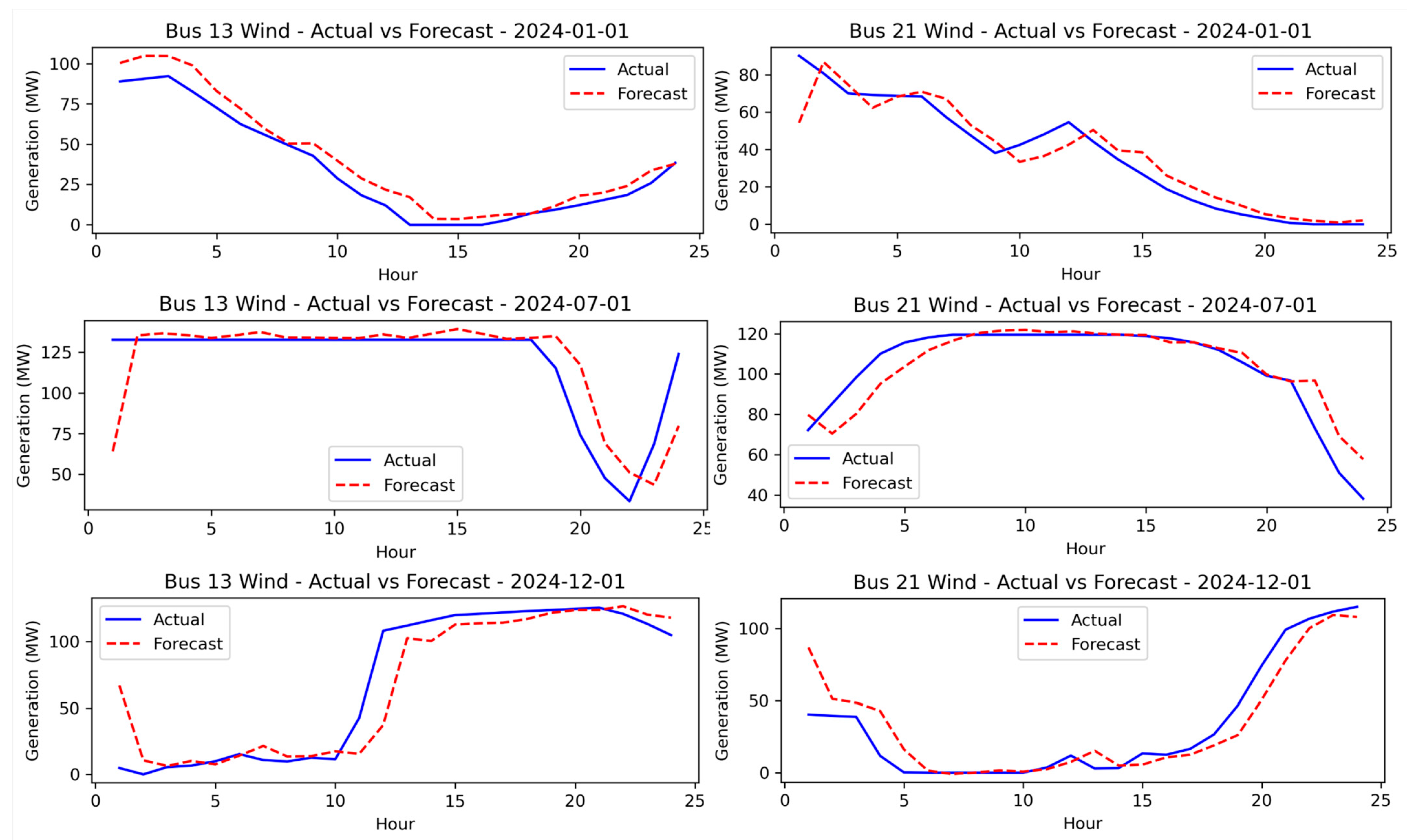
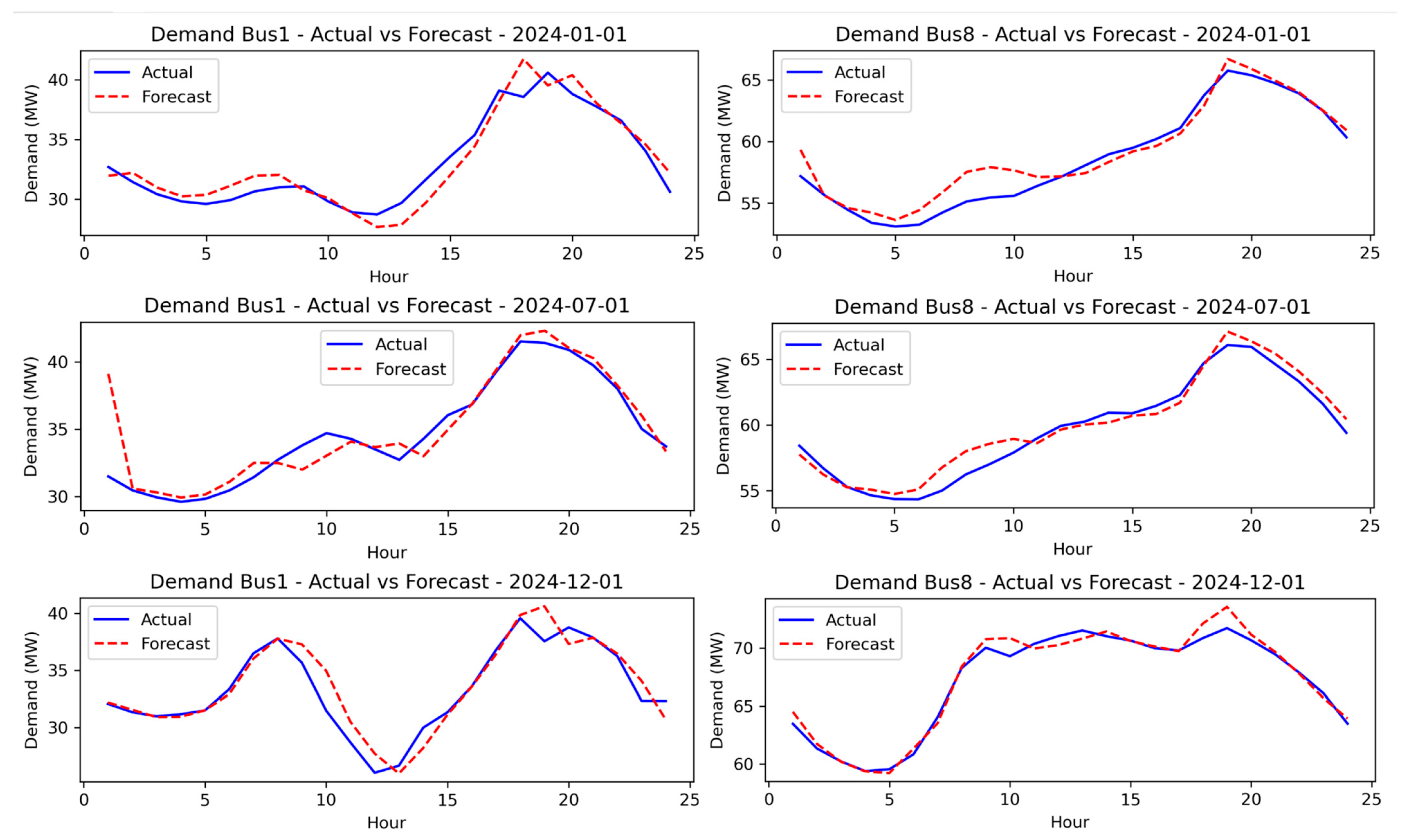
Seasonal analysis shows that wind forecast errors peak in winter due to weather variability, guiding adjustments in uncertainty sets. Solar generation rises in summer, influencing battery discharge strategies. The model’s coefficient of determination exceeds 0.90, and key features explain 85–92% of the variance, supporting reliable scheduling. Figure 2 analyzes solar generation. Stable patterns on February 1 show smooth integration, while cloud-related mismatches on 1 July (up to 20 MW) point to possible curtailments that the DDRO helps avoid. Ramp errors on 1 December highlight winter forecast challenges, reinforcing the use of residuals for bounding uncertainty. Figure 3 focuses on wind. Large underestimations on 1 January (up to 50 MW) suggest a need for reserves. More accurate fits on 1 July with 30 MW dips indicate better summer predictability. 1 December shows up to 20% underprediction, stressing the value of XGBoost in setting reliable baselines for ambiguity sets. Figure 4 reviews demand at Buses 1 and 8. Winter peaks show 10–15 MW forecast gaps due to heating loads, useful for planning load overruns. In contrast, summer deviations remain below 5 MW, confirming good performance under typical conditions. These findings demonstrate XGBoost’s effectiveness as a scalable forecasting tool. By delivering both point estimates and residuals, it supports robust OPF and enhances system reliability, enabling 15–25% renewable penetration with minimal curtailment.

4.2.2. Uncertainty Characterization

The data-driven uncertainty sets are central to robustness in the DDRO-OPF framework. They are derived from 2023 forecast residuals and do not rely on fixed probability distributions. For renewables, the 5th percentile of residuals sets a lower bound to guard against generation drops. For demand, the 95th percentile forms an upper bound to manage load surges. A minimum deviation of 0.05 MW is used to maintain numerical stability. These historical patterns form polyhedral ambiguity sets, enabling tractable reformulation of constraints via dualization, as discussed in Section 3. This non-parametric approach improves reliability to extreme events and reduces constraint violations by about 80%, with only a 5% increase in operational cost.
Hourly delta analysis confirms the framework’s ability to capture time-specific uncertainty. For example, Bus 13 wind shows deltas from 12.06 MW at hour 20 to 70.57 MW at hour 0, with an average of 17.89 MW and standard deviation of 13.45 MW. Hours 0–5 average 28.4 MW and show negative correlation with time. Bus 21 wind follows similar trends, averaging 16.2 MW with peaks up to 65.3 MW. PV deviations are lower, such as Bus 10 reaching 45.2 MW during cloudy midday hours. Demand deltas average 1.82 MW with a standard deviation of 0.62 MW. Bus 1 peaks at 4.70 MW at midnight, while hours 8–17 show morning and evening ramps averaging 2.1 MW. Table 6 summarizes these results, showing renewable variability to be five to six times higher than demand.
Demand uncertainty mostly comes from regular human behavior and weather trends, making it easier to forecast. This predictability works well with cyclical features, leading to relatively mean absolute errors below 2%. In contrast, renewables face more difficulty due to sudden weather changes like wind gusts and cloud cover, which cause large residual errors that are harder to predict. The DDRO framework helps manage this by protecting against extreme outcomes within the ambiguity set, reducing the need for reserve over-provisioning. With battery support, spinning reserves drop by 10–15%, and average exceedance remains below 15%, improving grid reliability as renewable penetration increases.
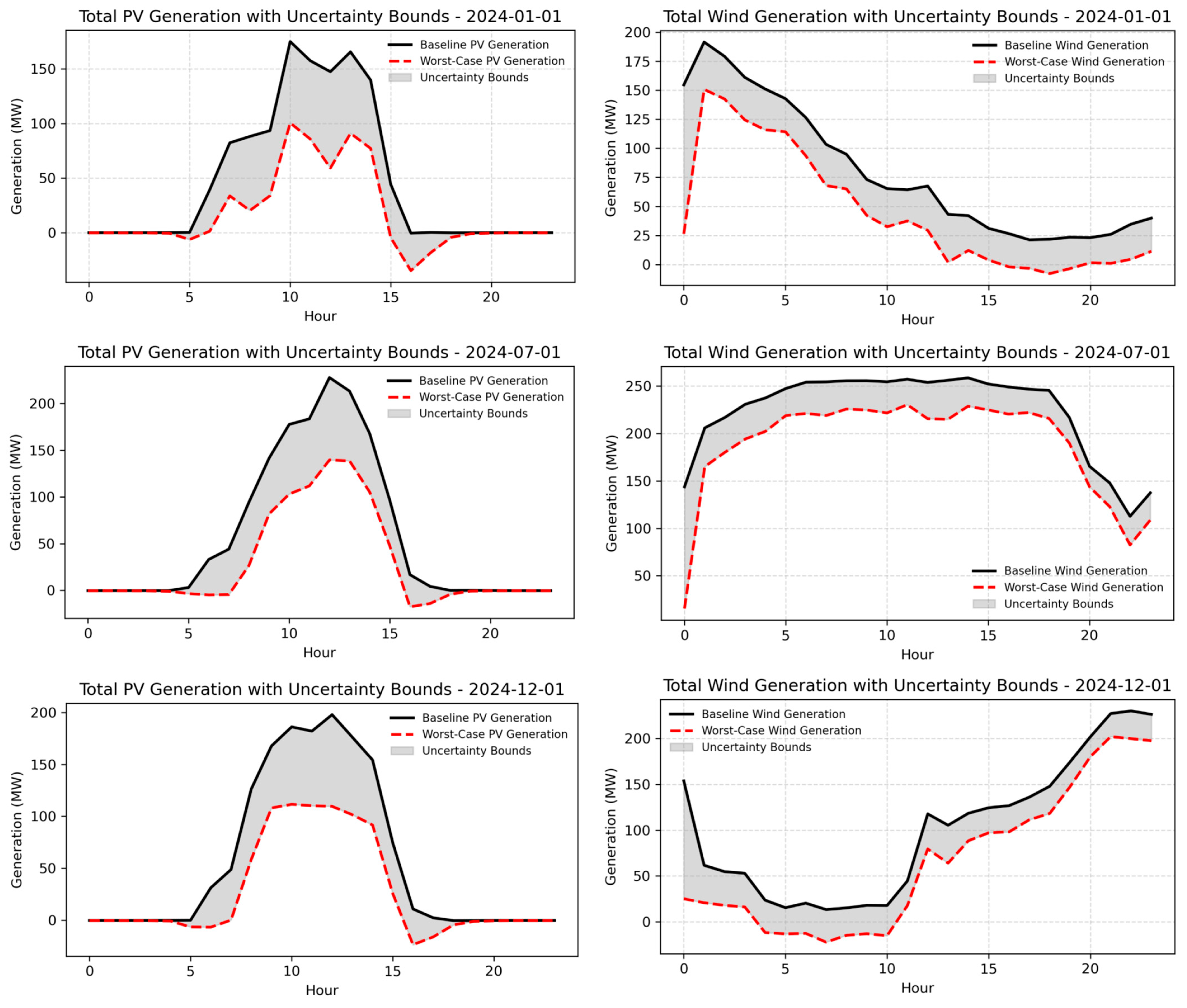
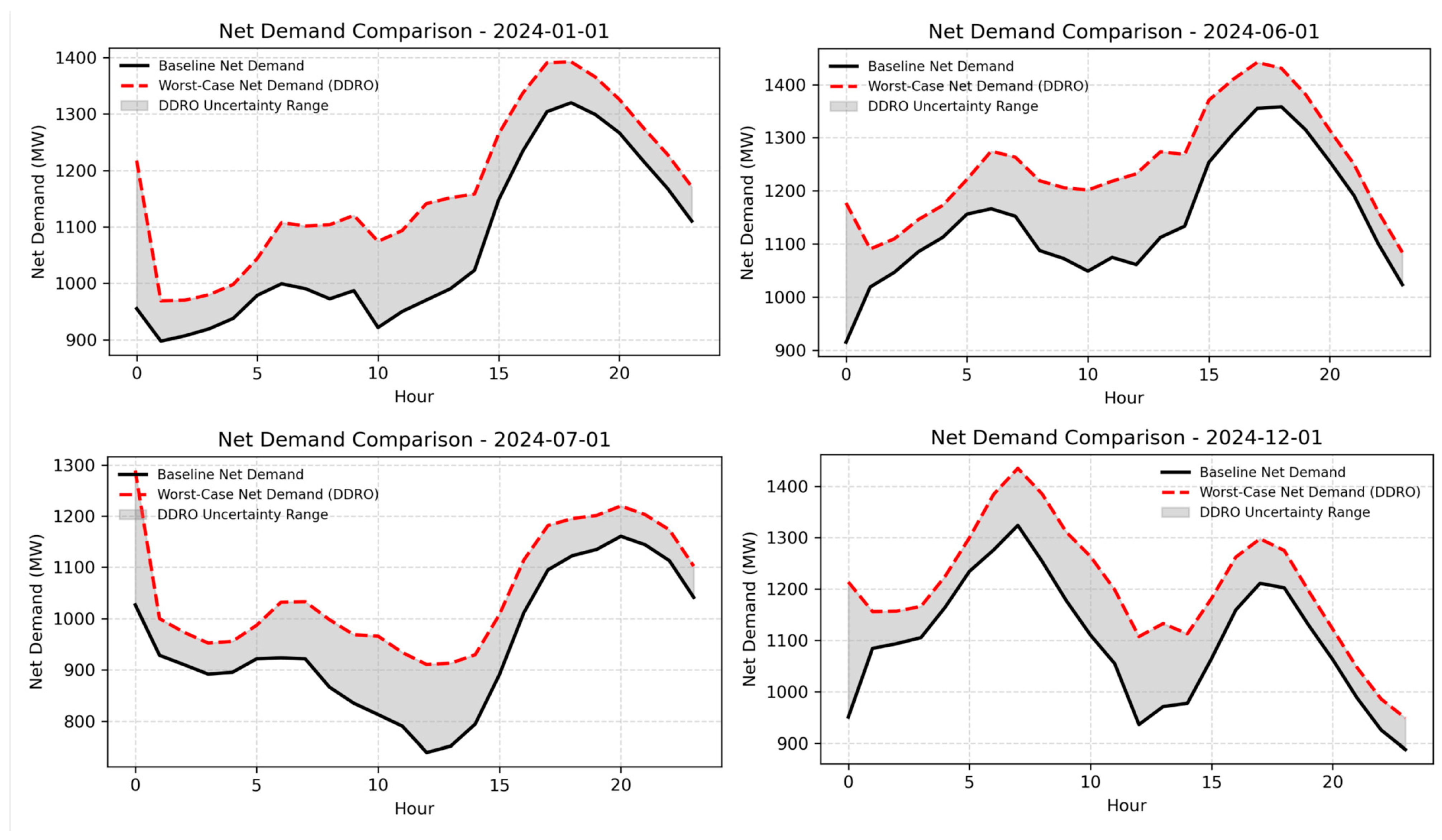
Figure 5 illustrates the uncertainty bounds for total PV and wind generation on 1 January, 1 July, and 1 December 2024. For PV, the bounds are narrow in the early morning and evening but widen significantly around midday in summer, with potential shortfalls of up to 50 MW due to rapid cloud cover. This highlights the need for ramping capacity, which the DDRO framework anticipates by preparing reserves that prevent curtailment. For wind, the seasonal effect is more pronounced. In winter months, the uncertainty bounds expand by as much as 100 MW during overnight hours, reflecting gusty and volatile wind conditions. By inflating the worst-case envelope during such periods, DDRO captures this variability and secures additional generation flexibility, effectively hedging against large seasonal swings. Across all tested days, actual PV and wind generation remains within the DDRO-derived bounds in 85–98% of hours, with only minor exceedances during extreme events such as December wind surges. This demonstrates that the bounds are neither overly conservative nor too optimistic, striking a balance between reliability and cost. Figure 6 further compares net demand forecasts for 1 January, 1 June, 1 July, and 1 December. During peak hours, DDRO raises the baseline net demand by 12–18% (approximately 100–200 MW), reflecting worst-case renewable shortfalls. For instance, in July, when wind shortfalls reached 150 MW, actual net demand nearly matched the DDRO envelope, confirming its role in capturing high-variability conditions. Figure 5 and Figure 6 illustrate exceedance rates, averaging 14.8% for renewables and 15.9% for demand. Seasonal peaks appear in July (25%) and June (23.8%), while lows occur in January. These patterns align with seasonal variability, and during high-exceedance months, the model dispatches up to 20% more resources to prevent blackouts at marginal additional cost.

4.2.3. Optimization Results

The DDRO-OPF model produces operational schedules that balance economic efficiency with reliability under uncertainty. Table 7 summarizes daily optimization metrics across 2024. The average daily operating cost is 280,241 USD, with a standard deviation of 15,200 USD. Distributed generation (DG) provides an average of 28,058 MW, supplying 82–90% of total demand. Renewable penetration averages 17.7%, ranging from 10.2% in January to 22.7% in May. Seasonal trends are evident: costs are higher in autumn and winter, reaching 300,514 USD in September due to reduced renewable output (−146 MW forecast error) and elevated demand overruns (+104 MW in November). In contrast, summer months benefit from higher PV availability, lowering daily costs to 253,129 USD in July. Correlation analysis confirms these drivers: a strong negative correlation (−0.68, p < 0.01) exists between actual renewable generation and operating costs, meaning greater renewable supply reduces reliance on costly DG. A positive correlation (0.52, p < 0.05) with demand deviations indicates that unexpected load overruns directly increase costs through additional ramping or shedding. Seasonal renewable deviations also follow a clear pattern. Spring (March–May) shows average surpluses of +178 MW, supporting efficient integration without curtailment. Summer and autumn shift to negative deviations (−119 MW on average), requiring DG output to increase by about 10% to cover shortfalls. Demand deviations are smaller in magnitude (≈49 MW on average) but can be substantial during peaks, such as +268 MW in April, which raised daily costs by nearly 10% due to the mobilization of reserves.
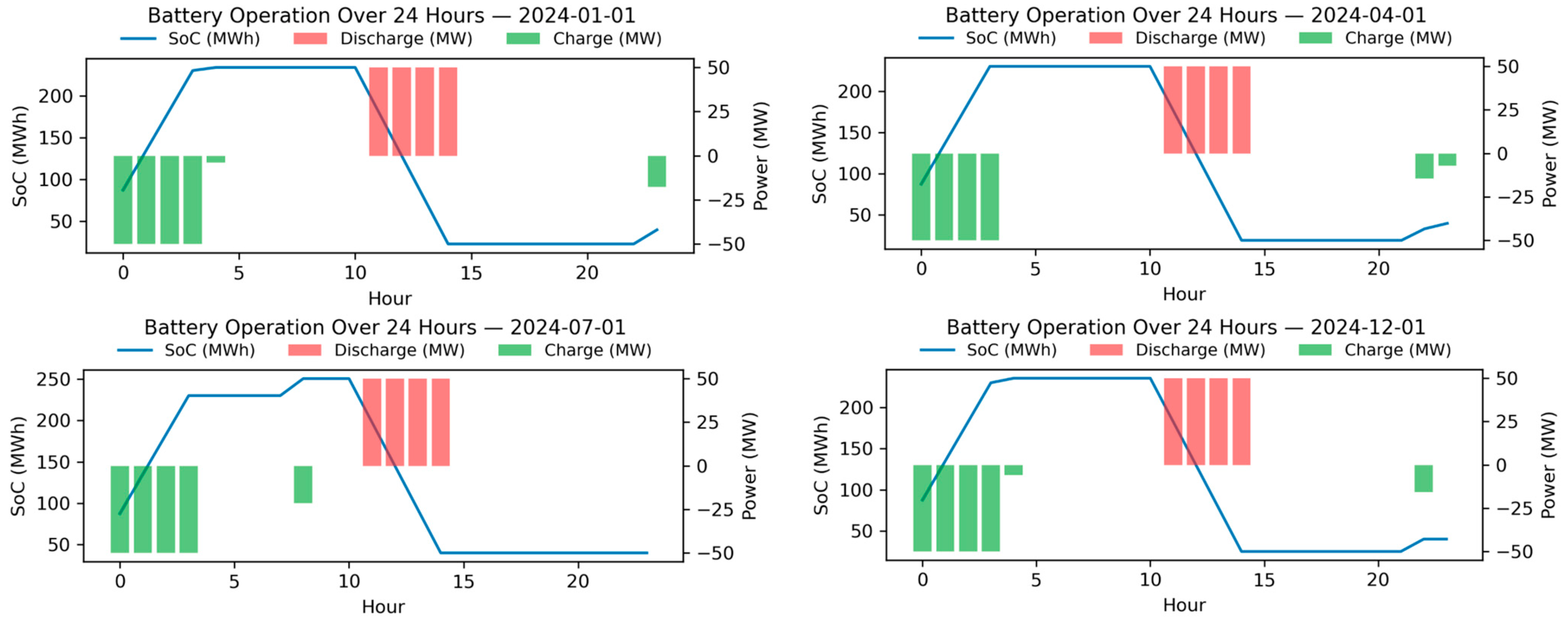
Battery energy storage plays a central role in managing these variations. On average, the BESS charges 221.6 MW and discharges 200 MW per day, yielding net flexibility of ~22 MW. Unlike the deterministic OPF, the DDRO framework maintains a systematically higher minimum state-of-charge, effectively reserving energy for uncertain peak hours. Figure 7 illustrates this behavior: charging is concentrated in early hours, while discharging is deferred to periods of high demand or large forecast uncertainty (hours 11–14). By doing so, the battery reduces dependence on fast-start DG units and achieves daily cost savings of about 5000 USD. Across the year, the BESS offsets up to 8% of net deviations during stress periods and maintains 10–15% higher reserves compared to deterministic scheduling.
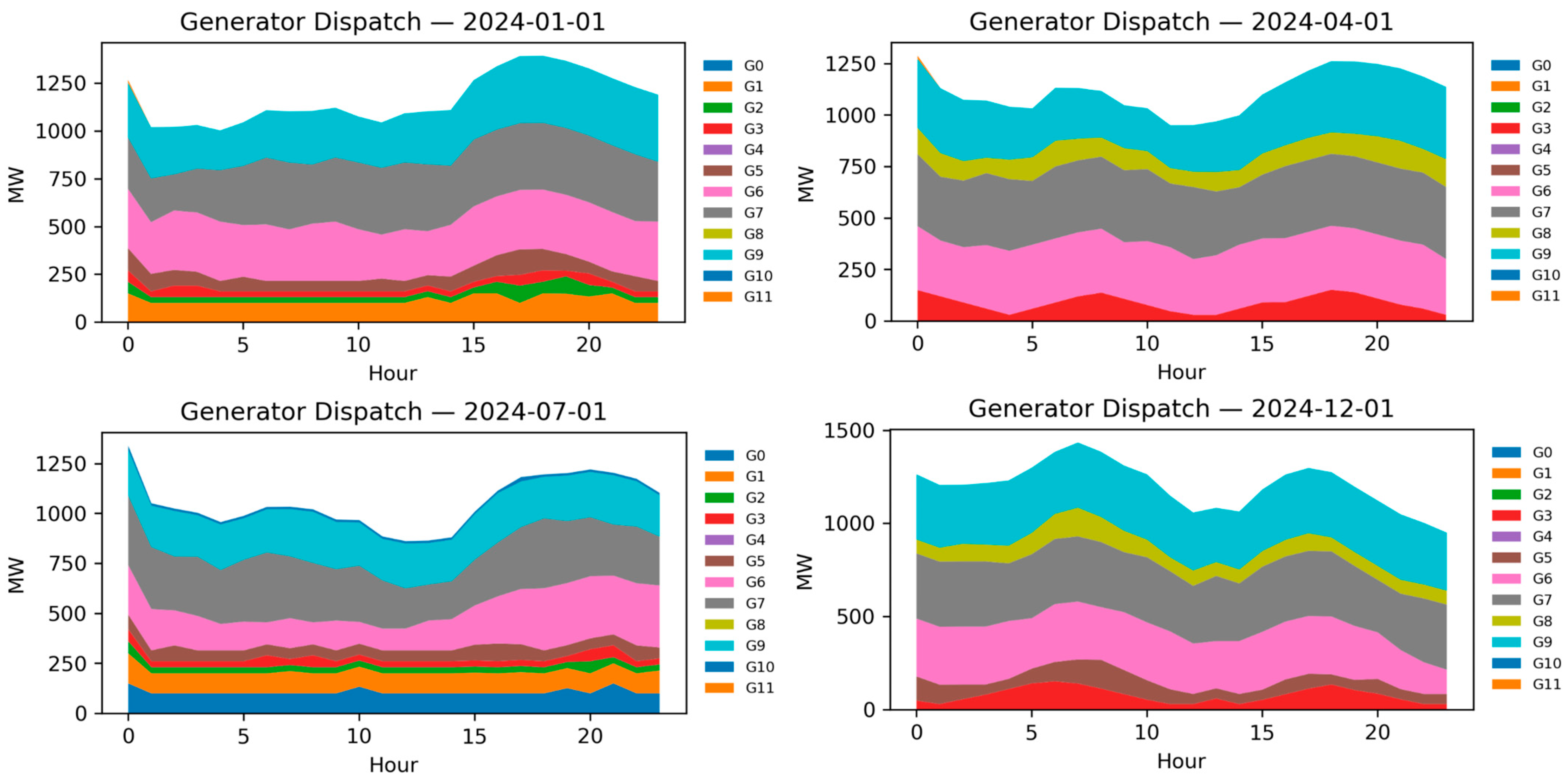
Load shedding remains minimal, below 10 MW per day (0.03% of demand), and occurs only in extreme cases, such as July, when renewable exceedance rates reached 25%. This performance represents about a 12% reduction in violations relative to deterministic OPF. Generator dispatch patterns in Figure 8 further demonstrate DDRO’s adaptive behavior: base-load units G1 and G2 dominate in low-renewable winter days, while flexible units G10–G12 provide backup during volatile conditions (e.g., 1 December). Summer operation in July relies more on PV support, reducing ramping stress on conventional units.
The DDRO framework achieves 15–25% renewable integration with less than 1% load shedding, improving upon deterministic baselines by 10–20% in terms of violations and reserve shortfalls. The BESS emerges as a pivotal resource, not only smoothing net load but also enabling risk-averse hedging strategies that balance cost and reliability in uncertain environments.

4.2.4. Benchmark Comparison with Stochastic and Robust Models

To highlight the relative advantages of the proposed DDRO framework, we implemented three benchmark models: a deterministic OPF baseline, a scenario-based stochastic formulation, and a Γ-robust formulation. The deterministic baseline corresponds to the same optimization model solved with ε = 0; i.e., the ambiguity set collapses to the empirical point forecasts, and no uncertainty margins are applied. While this optimistic reference produces the lowest possible operating cost, it is unrealistic in practice as it provides no protection against forecast errors.
The stochastic formulation minimizes expected operating cost across 100 scenarios of wind, PV, and demand, sampled from historical residuals and reduced for tractability. The Γ-robust model enforces feasibility against simultaneous worst-case deviations in a subset of uncertain parameters, with Γ set to 20% following common practice in robust optimization studies. This choice provides protection against significant variability without being overly conservative. Table 8 reports the average daily costs and exceedance rates for the four approaches across the twelve representative horizons.
The deterministic formulation produces the lowest daily cost but is consistently unreliable, with exceedance rates above 20% for both renewable and demand realizations. The stochastic formulation achieves moderate improvements in reliability by explicitly modeling variability, but still allows substantial exceedances in highly volatile months. The Γ-robust formulation reduces exceedances to near 11% but does so at a significant cost premium, with daily costs rising above 305k USD on average.
The proposed DDRO method provides the most balanced outcome. Its cost (≈289k USD) is much closer to the stochastic model than to the robust benchmark, yet its exceedance rates (14.8% for renewables and 15.9% for demand) approach those of the robust model. This confirms that DDRO effectively reduces forecast uncertainty violations without incurring the excessive conservatism of classical robust optimization. The benchmark results therefore demonstrate that DDRO achieves a superior cost–reliability trade-off compared to both stochastic and robust approaches, validating its practical value for transmission system operation under uncertainty.

4.2.5. Sensitivity to Wasserstein Radius, Cost-Scaling Parameter, and Percentile Bounds

The conservatism of the DDRO formulation is primarily controlled by two hyperparameters: the Wasserstein radius (ε) and the transport-cost scale ( η c ). Both parameters influence how aggressively the model hedges against uncertainty, directly affecting operating cost, reliability, and solution tractability. To examine their impact, we conducted a sensitivity analysis by varying ε ∈ {0.5, 1.0, 2.0} and η c ∈ {0.02, 0.05, 0.10} while solving the same twelve representative daily horizons. Table 9 summarizes the average daily total cost, renewable and demand exceedance rates, and average solution time across these tests.
The results demonstrate clear trends. A smaller Wasserstein radius (ε = 0.5) yields optimistic schedules with the lowest cost (≈276k USD) but poor reliability, as exceedance rates rise to ~20%. A larger radius (ε = 2.0) produces very conservative dispatch decisions, reducing exceedances to ~12% but increasing daily cost above 300k USD. The intermediate value (ε = 1.0) offers a balanced outcome, maintaining cost within 289k USD while limiting exceedances to 14–16%.
Similarly, adjusting the transport scale η c shifts the trade-off. A smaller value ( η c = 0.02) weakens robustness, lowering cost slightly but worsening exceedances, while a larger value ( η c = 0.10) enforces stricter penalties on deviations, reducing exceedances to ~13% at the expense of higher cost (~295k USD). Across all cases, solution times remained under 5 min per daily horizon, confirming computational tractability.
In addition to ε and η c , we also examined the impact of the percentile thresholds used to define renewable and demand uncertainty bounds. The main case adopts the 5th–95th percentiles of forecast residuals to balance cost and reliability. Table 10 compares this choice with narrower (10th–90th) and wider (2.5th–97.5th) bounds.
The results confirm the expected trade-off: tighter bounds (10th–90th) reduce cost but increase exceedance rates, while wider bounds (2.5th–97.5th) improve reliability at the expense of higher cost. The 5th–95th percentiles provide a balanced middle ground and were therefore selected as the baseline case. This choice is also consistent with common practice in data-driven uncertainty modeling, where intermediate quantiles are used to avoid both extreme outliers and underrepresentation of risk.

4.2.6. Computational Performance and Scalability

To evaluate tractability, the DDRO model was solved for twelve representative daily cases on the 24-bus system. All simulations were performed on a workstation with an Intel Core i7-11700 processor (2.50 GHz, 8 cores, 16 threads) and 16 GB RAM, running Windows 11 Enterprise, using Gurobi 11.0 as the MILP solver. The average solution time for each daily case ranged between 85 and 130 s, with the most complex cases not exceeding 150 s. Runtime variability primarily depended on the level of renewable forecast errors and demand deviations. Table 11 summarizes the solution times across months, showing that cases with higher exceedance rates (e.g., July and June) generally required longer optimization runs.
These results indicate that the proposed formulation is computationally efficient for medium-scale systems with integrated renewables and storage. Across all cases, the daily horizon was solved within a few minutes, confirming the practicality of the model for operational planning. However, scaling to larger grids with hundreds of buses would substantially increase problem size due to hourly unit commitment, binary variables, and uncertainty dimensions. Potential remedies include decomposition methods, such as Benders decomposition, to separate unit commitment from network constraints; parallel computing, where daily or scenario subproblems are solved simultaneously; and progressive hedging or ADMM-based approaches, which partition the problem by time or uncertainty scenarios. Combining these techniques with high-performance solvers can extend the applicability of the proposed DDRO framework to larger, real-world transmission systems while maintaining tractability.

5. Conclusions

This paper introduces a novel data-driven DDRO-OPF framework designed to address the increasing challenges of renewable energy variability and demand uncertainty in modern power systems. The framework integrates accurate forecasting using XGBoost, empirical modeling of uncertainty through residual analysis, and robust optimization using polyhedral ambiguity sets based on the Wasserstein distance. These elements enable the system to remain reliable and economically efficient even under worst-case scenarios. The proposed method constructs ambiguity sets directly from the residuals of forecast errors, avoiding assumptions about the exact distribution of uncertainties. These sets are then used to reformulate the optimization problem into a tractable and solvable form. This approach ensures that the power system operates safely and cost-effectively, even when faced with unexpected variations in renewable output or electricity demand. The framework is tested on the IEEE 24-bus benchmark system using representative days from the year 2024. The results demonstrate its strong performance in both prediction and optimization tasks. The XGBoost forecasting model delivers high accuracy, with relative mean absolute errors under 5% for renewable generation and below 2% for demand. It captures 85–92% of the variance in the data by leveraging time-based features such as cyclical patterns and lag values. These high-quality forecasts form the foundation for building reliable and realistic uncertainty sets. The uncertainty sets effectively model time-dependent fluctuations. The DDRO framework keeps the average exceedance rate below 15% and reduces constraint violations by about 80% when compared to traditional point-forecast-based OPF models. These benefits are achieved with only a 5% increase in operational cost, making the approach practical and scalable for real-world applications. The optimization model achieves an average daily operating cost of $280,241. It supports an average renewable energy share of 17.7%, reaching as high as 22.7% during peak months like May. The DDRO-OPF model improves the balance between cost and reliability by 10–20%, confirming its value as a decision-making tool for grid operators. It supports higher integration of variable renewable sources while maintaining system stability and affordability. A limitation of this study is the use of hour-wise (rectangular) ambiguity sets, which do not capture temporal correlations across consecutive periods. Future research could address this by developing joint or block-residual Wasserstein sets, copula-based models, or deviation-budget approaches to better represent persistence while maintaining tractability.

Author Contributions

Conceptualization, M.G.; methodology, M.G.; modeling and simulation, M.G.; validation, M.G., D.H. and A.A.; formal analysis, M.G., D.H. and A.A.; investigation, M.G., D.H. and A.A.; writing, original draft preparation, M.G.; writing, review and editing, D.H., and A.A.; visualization, M.G.; supervision, D.H. and A.A. All authors have read and agreed to the published version of the manuscript.

Funding

This research received no external funding.

Data Availability Statement

The original contributions presented in this study are included in the article. Further inquiries can be directed to the corresponding author.

Conflicts of Interest

The authors declare no conflicts of interest.

Nomenclature

SymbolDescriptionSymbolDescription
T Set of time periods (hours) S o C t Battery state-of-charge at end of hour t (%)
G Set of thermal generators P t c h Battery charging power at hour t (MW)
B Set of buses P t dch   Battery discharging power at hour t (MW)
L Set of directed network lines c g Marginal cost of generator g (MWh)
H c h Set of preferred battery charging hours C L S Load-shedding penalty cost (USD/MWh)
H dch Set of preferred battery discharging hours C b D R Demand-response cost coefficient at bus b ( U S D / M W h )
R Set of renewable resources (wind and PV) α c h , α d c h BESS charging/discharging incentives ( U S D / M W h )
D Set of demand resources P g max   , P g min   Maximum/minimum capacity of generator g (MW)
I Set of all uncertain resources ( R D ) R g U , R g D Ramp-up/down limits of generator g (MW/h)
P g , t Power output of generator g at hour t (MW) M U T g , M D T g Minimum up-time/down-time of generator g
u g , t Binary on/off status of generator g at hour t η Battery round-trip efficiency
S U g , t Binary startup indicator for generator g at hour t P ch ,   dch , max   Maximum BESS charge/discharge rates (MW)
S D g , t Binary shutdown indicator for generator g at hour t X i j Reactance of line ( i , j ) (pu)
L S b , t Load shedding at bus b , hour t (MW) B i j = 1 / X i j Susceptance of line ( i , j ) (pu)
A b collector area at bus b   m 2 F i j m a x Thermal limit of line (i,j) (MW)
z t Binary battery mode at hour t ( 1 = charge, 0 = discharge) v b c i , v b r , v b c o Cut-in/rated/cut-out wind speeds at bus b (m/s)
F i j , t Power flow on line ( i , j ) at hour t (MW) P b W ,   max   Rated wind capacity at bus b (MW)
θ b , t Voltage-phase angle at bus b , hour t (rad) η P V PV module efficiency
δ b , t D Demand deviation recourse at bus b r   hour t (MW) P b P V , m a x Nameplate PV capacity at bus b (MW)
δ b , t R Renewable deviation recourse at bus b , hour t (MW) Δ P b _ , Δ P b ¯ DR adjustment Min and Max bounds at bus b (MW)
λ Dual multiplier for Wasserstein-ball radius δ min   Minimum uncertainty margin (MW)
ζ t Auxiliary dual variable for DRO at hour t ε Wasserstein-ball radius (MW)
Δ P b , t D R Demand-response adjustment at bus b and hour t (MW) η c Ground-metric (transport) scale in the chosen L 1 cost used for the Wasserstein distance
N Number of validation residual samples ε i , t Forecast residual of resource i at hour t (MW)
P Wasserstein ambiguity set Q p ( ) Empirical p -quantile operator
P ^ Empirical distribution of residuals P b , t D ,   fore   Forecast demand at bus b r hour t (MW)

Appendix A

Appendix A.1. Derivation of the Surrogate Dual Reformulation

We provide a derivation sketch for the surrogate dual used in Section 3.4. The starting point is the standard DRO problem with Wasserstein ambiguity sets:
s u p Q P   E ε Q [ f ( ε ) ] , P = Q W c ( Q , P ^ ) ε
where P ^ is the empirical distribution of residuals, W c ( , ) is the Wasserstein distance with ground metric c ( , ) , and ε 0 is the radius of the ambiguity set. By the Kantorovich–Rubinstein duality, this admits the reformulation:
s u p Q : W c ( Q , P ^ ) ε   E Q [ f ( ξ ) ] = m i n λ 0   λ ε + 1 N n = 1 N     s u p ξ   f ( ξ ) λ c ξ , ξ ( n )

Appendix A.2. Choice of Recourse Loss and Ground Metric

In our model, the recourse loss is defined as a linear penalty on deviations:
f ( ξ ) = t T   f t ξ t , f t ξ t = b B   δ b , t D + δ b , t R
where δ b , t D and δ b , t R are the deviation variables for demand and renewable shortfall at bus b and time t . The ground metric is chosen as an L 1 distance with a transport-cost scale η c :
c t ξ t , ξ t ( n ) = η c ξ t ξ t ( n ) 1
where η c is a dimensionless scaling factor in normalized residual space. It controls the cost of transporting probability mass between realizations and therefore governs the trade-off between robustness and cost.

Appendix A.3. Surrogate Reformulation

Applying (A2) with the separable loss (A3) and ground metric (A4) yields for each time t :
s u p ξ t   f t ξ t λ c t ξ t , ξ t ( n ) b   δ b , t D + δ b , t R λ η c
This upper bound corresponds to the Lipschitz envelope of the inner maximization, which avoids introducing sample-indexed auxiliary variables. To linearize this expression, we introduce per-period auxiliaries ζ t such that:
ζ t b B   δ b , t D + δ b , t R λ η c , t T
Substituting into (A2) gives the tractable surrogate dual:
m i n x X , λ 0 , ζ t 0   C ( x ) + λ ε + t T   ζ t ,
which corresponds to Equations (24)–(28) in the main text.

Appendix A.4. Interpretation

  • λ is the dual variable associated with the Wasserstein radius, ε penalizing the distance from the empirical distribution.
  • ε controls the size of the ambiguity set: larger values increase conservatism.
  • η c is the transport-cost scale in the ground metric: larger values enforce stricter penalties on deviations, also increasing conservatism.
  • ζ t are auxiliary variables bounding the worst-case deviation cost at each time t.
Together, the pair ε , η c govern the model’s balance between economic efficiency and reliability.

References

  1. Cavus, M. Advancing Power Systems with Renewable Energy and Intelligent Technologies: A Comprehensive Review on Grid Transformation and Integration. Electronics 2025, 14, 1159. [Google Scholar] [CrossRef]
  2. Ghahramani, M.; Habibi, D.; Ghamari, S.; Aziz, A. Optimal Operation of an Islanded Hybrid Energy System Integrating Power and Gas Systems. IEEE Access 2024, 12, 196591–196608. [Google Scholar] [CrossRef]
  3. Soleimani, H.; Habibi, D.; Ghahramani, M.; Aziz, A. Strengthening power systems for net zero: A review of the role of synchronous condensers and emerging challenges. Energies 2024, 17, 3291. [Google Scholar] [CrossRef]
  4. Ghahramani, M.; Sadat-Mohammadi, M.; Nazari-Heris, M.; Asadi, S.; Mohammadi-Ivatloo, B. Introduction and literature review of the operation of multi-carrier energy networks. In Planning and Operation of Multi-Carrier Energy Networks; Springer: Berlin/Heidelberg, Germany, 2021; pp. 39–57. [Google Scholar]
  5. Ghahramani, M.; Habibi, D.; Ghamari, S.; Soleimani, H.; Aziz, A. Renewable-Based Isolated Power Systems: A Review of Scalability, Reliability, and Uncertainty Modeling. Clean Technol. 2025, 7, 80. [Google Scholar] [CrossRef]
  6. Zhao, Y.; Wei, Y.; Zhang, S.; Guo, Y.; Sun, H. Multi-objective robust optimization of integrated energy system with hydrogen energy storage. Energies 2024, 17, 1132. [Google Scholar] [CrossRef]
  7. Liang, J.; Miao, J.; Sun, L.; Zhao, L.; Wu, J.; Du, P.; Cao, G.; Zhao, W. Supply–Demand Dynamics Quantification and Distributionally Robust Scheduling for Renewable-Integrated Power Systems with Flexibility Constraints. Energies 2025, 18, 1181. [Google Scholar] [CrossRef]
  8. Lu, G.; Yuan, B.; Nie, B.; Xia, P.; Wu, C.; Sun, G. Enhanced dynamic expansion planning model incorporating Q-Learning and distributionally robust optimization for resilient and Cost-Efficient distribution networks. Energies 2025, 18, 1020. [Google Scholar] [CrossRef]
  9. Cai, P.; Wen, C.; Cao, B.; Qiao, J. A Wasserstein metric distributionally robust chance-constrained peer aggregation energy sharing mechanism for hydrogen-based microgrids considering low-carbon drivers. Energy 2025, 325, 136178. [Google Scholar] [CrossRef]
  10. Hao, J.; Guo, X.; Li, Y.; Wu, T. Uncertain scheduling of the power system based on wasserstein distributionally robust optimization and improved differential evolution algorithm. Energies 2024, 17, 3846. [Google Scholar] [CrossRef]
  11. Yin, C.; Dong, J.; Zhang, Y. Distributionally Robust Bilevel Optimization Model for Distribution Network with Demand Response under Uncertain Renewables Using Wasserstein Metrics. IEEE Trans. Sustain. Energy 2024, 16, 1165–1176. [Google Scholar] [CrossRef]
  12. Yuan, Y.; Zhang, H.; Zhang, S.; Cheng, H.; Chen, F.; Wang, Z.; Zhang, X. A multi-scenario distributionally robust model for resilience-oriented offshore wind farms and transmission network integrated planning considering typhoon disasters. Appl. Energy 2025, 392, 125937. [Google Scholar] [CrossRef]
  13. Singh, U.; Rizwan, M.; Alaraj, M.; Alsaidan, I. A machine learning-based gradient boosting regression approach for wind power production forecasting: A step towards smart grid environments. Energies 2021, 14, 5196. [Google Scholar] [CrossRef]
  14. Ghahramani, M.; Nazari-Heris, M.; Zare, K.; Mohammadi-ivatloo, B. Robust short-term scheduling of smart distribution systems considering renewable sources and demand response programs. In Robust Optimal Planning and Operation of Electrical Energy Systems; Springer: Berlin/Heidelberg, Germany, 2019; pp. 253–270. [Google Scholar]
  15. Ghahramani, M.; Nazari-Heris, M.; Zare, K.; Mohammadi-Ivatloo, B. Energy and reserve management of a smart distribution system by incorporating responsive-loads/battery/wind turbines considering uncertain parameters. Energy 2019, 183, 205–219. [Google Scholar] [CrossRef]
  16. Ghahramani, M.; Habibi, D.; Ghamari, S.; Aziz, A.; Ghahramani, M.; Habibi, D.; Ghamari, S.; Aziz, A. Addressing Uncertainty in Renewable Energy Integration for Western Australia’s Mining Sector: A Robust Optimization Approach. Energies 2024, 17, 5679. [Google Scholar] [CrossRef]
  17. Khaloie, H.; Dolanyi, M.; Toubeau, J.-F.; Vallée, F. Review of machine learning techniques for optimal power flow. Appl. Energy 2025, 388, 125637. [Google Scholar] [CrossRef]
  18. Jamal, R.; Khan, N.H.; Ebeed, M.; Zeinoddini-Meymand, H.; Shahnia, F. An improved pelican optimization algorithm for solving stochastic optimal power flow problem of power systems considering uncertainty of renewable energy resources. Results Eng. 2025, 26, 104553. [Google Scholar] [CrossRef]
  19. Ghahramani, M.; Heris, M.N.; Zare, K.; Ivatloo, B.M. Robust Optimization of Renewable Energy Based Distribution Networks Considering Electrical Energy Storage and Fuel Cell. In Proceedings of the Electrical Engineering (ICEE), Iranian Conference on, Mashhad, Iran, 8–10 May 2018; pp. 1343–1349. [Google Scholar]
  20. Shui, Y.; Gao, H.; Wang, L.; Wei, Z.; Liu, J. A data-driven distributionally robust coordinated dispatch model for integrated power and heating systems considering wind power uncertainties. Int. J. Electr. Power Energy Syst. 2019, 104, 255–258. [Google Scholar] [CrossRef]
  21. Zhang, S.; Qiu, G.; Liu, Y.; Ding, L.; Shui, Y.; Zhang, S.; Qiu, G.; Liu, Y.; Ding, L.; Shui, Y. Data-Driven Distributionally Robust Optimization-Based Coordinated Dispatching for Cascaded Hydro-PV-PSH Combined System. Electronics 2024, 13, 667. [Google Scholar] [CrossRef]
  22. Zhou, Y.; Hou, H.; Yan, H.; Wang, X.; Zhou, R. Data-driven distributionally robust stochastic optimal dispatching method of integrated energy system considering multiple uncertainties. Energy 2025, 325, 136104. [Google Scholar] [CrossRef]
  23. Li, Y.; Han, M.; Shahidehpour, M.; Li, J.; Long, C. Data-driven distributionally robust scheduling of community integrated energy systems with uncertain renewable generations considering integrated demand response. Appl. Energy 2023, 335, 120749. [Google Scholar] [CrossRef]
  24. Liu, H.; Qiu, J.; Zhao, J. A data-driven scheduling model of virtual power plant using Wasserstein distributionally robust optimization. Int. J. Electr. Power Energy Syst. 2022, 137, 107801. [Google Scholar] [CrossRef]
  25. Saberi, H.; Zhang, C.; Dong, Z.Y. Data-driven distributionally robust hierarchical coordination for home energy management. IEEE Trans. Smart Grid 2021, 12, 4090–4101. [Google Scholar] [CrossRef]
  26. Parvar, S.S.; Nazaripouya, H. Optimal Operation of Battery Energy Storage Under Uncertainty Using Data-Driven Distributionally Robust Optimization. Electr. Power Syst. Res. 2022, 211, 108180. [Google Scholar] [CrossRef]
  27. Li, H.; Lu, X.; Zhou, K.; Shao, Z. Distributionally robust optimal dispatching method for integrated energy system with concentrating solar power plant. Renew. Energy 2024, 229, 120792. [Google Scholar] [CrossRef]
  28. Zhang, X.; Liang, Z.; Chen, S. Optimal low-carbon operation of regional integrated energy systems: A data-driven hybrid stochastic-distributionally robust optimization approach. Sustain. Energy Grids Netw. 2023, 34, 101013. [Google Scholar] [CrossRef]
  29. Han, J.; Han, K.; Han, T.; Wang, Y.; Han, Y.; Lin, J. Data-driven distributionally robust optimization of low-carbon data center energy systems considering multi-task response and renewable energy uncertainty. J. Build. Eng. 2025, 102, 111937. [Google Scholar] [CrossRef]
  30. Shi, Z.; Zhang, T.; Liu, Y.; Feng, Y.; Wang, R.; Huang, S. Energy management of multi-microgrid system with renewable energy using data-driven distributionally robust optimization. Int. J. Green Energy 2024, 21, 2699–2711. [Google Scholar] [CrossRef]
  31. Zhang, X.; Ge, S.; Liu, H.; Zhou, Y.; He, X.; Xu, Z. Distributionally robust optimization for peer-to-peer energy trading considering data-driven ambiguity sets. Appl. Energy 2023, 331, 120436. [Google Scholar] [CrossRef]
  32. Li, J.; Khodayar, M.E.; Wang, J.; Zhou, B. Data-driven distributionally robust co-optimization of P2P energy trading and network operation for interconnected microgrids. IEEE Trans. Smart Grid 2021, 12, 5172–5184. [Google Scholar] [CrossRef]
  33. Duan, C.; Jiang, L.; Fang, W.; Liu, J.; Liu, S. Data-driven distributionally robust energy-reserve-storage dispatch. IEEE Trans. Ind. Inform. 2017, 14, 2826–2836. [Google Scholar] [CrossRef]
  34. Wang, H.; Yi, Z.; Xu, Y.; Cai, Q.; Li, Z.; Wang, H.; Bai, X. Data-driven distributionally robust optimization approach for the coordinated dispatching of the power system considering the correlation of wind power. Electr. Power Syst. Res. 2024, 230, 110224. [Google Scholar] [CrossRef]
  35. Gurumoorthi, G.; Senthilkumar, S.; Karthikeyan, G.; Alsaif, F.; Gurumoorthi, G.; Senthilkumar, S.; Karthikeyan, G.; Alsaif, F. A hybrid deep learning approach to solve optimal power flow problem in hybrid renewable energy systems. Sci. Rep. 2024, 14, 19377. [Google Scholar] [CrossRef] [PubMed]
  36. Hasanien, H.M.; Alsaleh, I.; Ullah, Z.; Alassaf, A. Probabilistic optimal power flow in power systems with Renewable energy integration using Enhanced walrus optimization algorithm. Ain Shams Eng. J. 2024, 15, 102663. [Google Scholar] [CrossRef]
  37. Mouassa, S.; Alateeq, A.; Alassaf, A.; Bayindir, R.; Alsaleh, I.; Jurado, F. Optimal power flow analysis with renewable energy resource uncertainty using dwarf mongoose optimizer: Case of ADRAR isolated electrical network. IEEE Access 2024, 12, 10202–10218. [Google Scholar] [CrossRef]
  38. Mahmoodi, M.; RA, S.M.N.; Blackhall, L.; Scott, P. A comparison on power flow models for optimal power flow studies in integrated medium-low voltage unbalanced distribution systems. Sustain. Energy Grids Netw. 2024, 38, 101339. [Google Scholar] [CrossRef]
  39. Dai, X.; Zhai, J.; Jiang, Y.; Guo, Y.; Jones, C.N.; Hagenmeyer, V. Advancing distributed AC optimal power flow for integrated transmission-distribution systems. IEEE Trans. Netw. Sci. Eng. 2025, 12, 1210–1223. [Google Scholar] [CrossRef]
  40. Tiwari, D.; Zideh, M.J.; Talreja, V.; Verma, V.; Solanki, S.K.; Solanki, J. Power flow analysis using deep neural networks in three-phase unbalanced smart distribution grids. IEEE Access 2024, 12, 29959–29970. [Google Scholar] [CrossRef]
  41. Hussan, U.; Wang, H.; Ayub, M.A.; Rasheed, H.; Majeed, M.A.; Peng, J.; Jiang, H. Decentralized stochastic recursive gradient method for fully decentralized OPF in multi-area power systems. Mathematics 2024, 12, 3064. [Google Scholar] [CrossRef]
  42. Fu, X.; Zhang, C.; Xu, Y.; Zhang, Y.; Sun, H. Statistical machine learning for power flow analysis considering the influence of weather factors on photovoltaic power generation. IEEE Trans. Neural Netw. Learn. Syst. 2024, 36, 5348–5362. [Google Scholar] [CrossRef]
  43. Zhao, Y.; Gan, W.; Yan, M.; Wen, J.; Zhou, Y. A scalable stochastic scheme for identifying critical substations considering the epistemic uncertainty of contingency in power systems. Appl. Energy 2025, 381, 125119. [Google Scholar] [CrossRef]
  44. Guo, Y.; Baker, K.; Dall’Anese, E.; Hu, Z.; Summers, T.H. Data-based distributionally robust stochastic optimal power flow—Part I: Methodologies. IEEE Trans. Power Syst. 2018, 34, 1483–1492. [Google Scholar] [CrossRef]
  45. Li, H.; Liu, H.; Ma, J.; Li, D.; Zhang, W. Distributionally robust optimal dispatching method of integrated electricity and heating system based on improved Wasserstein metric. Int. J. Electr. Power Energy Syst. 2023, 151, 109120. [Google Scholar] [CrossRef]
  46. Zhai, J.; Wang, S.; Guo, L.; Jiang, Y.; Kang, Z.; Jones, C.N. Data-driven distributionally robust joint chance-constrained energy management for multi-energy microgrid. Appl. Energy 2022, 326, 119939. [Google Scholar] [CrossRef]
  47. Wang, H.; Bie, Z. Data-Driven Distributionally Robust Energy and Reserve Scheduling Considering RES Flexibility. IEEE Trans. Power Syst. 2024, 40, 2438–2450. [Google Scholar] [CrossRef]
  48. Liu, L.; Hu, Z.; Duan, X.; Pathak, N. Data-driven distributionally robust optimization for real-time economic dispatch considering secondary frequency regulation cost. IEEE Trans. Power Syst. 2021, 36, 4172–4184. [Google Scholar] [CrossRef]
  49. Zishan, F.; Akbari, E.; Montoya, O.D. Analysis of probabilistic optimal power flow in the power system with the presence of microgrid correlation coefficients. Cogent Eng. 2024, 11, 2292325. [Google Scholar] [CrossRef]
  50. ALAhmad, A.K.; Verayiah, R.; Ramasamy, A.; Shareef, H. Enhancing optimization accuracy in power systems: Investigating correlation effects on objective function values. Results Eng. 2024, 22, 102351. [Google Scholar] [CrossRef]
  51. Shah, A.A.; Wang, S.C.; Liu, G.; Hassan, R.U.; Nawaz, A. Scenario Based Optimal Power Flow Evaluation for Wind Power Allocation Capacity in Modern Power Systems. IEEE Access 2025, 13, 38443–38453. [Google Scholar] [CrossRef]
  52. Liu, J.; Zhang, S. Stochastic two-stage multi-objective unit commitment of distributed resource energy systems considering uncertainties and unit failures. Reliab. Eng. Syst. Saf. 2025, 253, 110520. [Google Scholar] [CrossRef]
  53. Jain, T.; Verma, K. Reliability enhancement with coordinated operation of wind power and battery energy storage using machine learning based unit commitment decision. J. Energy Storage 2025, 111, 115455. [Google Scholar] [CrossRef]
  54. Taheri, B.; Molzahn, D.K. Optimizing parameters of the DC power flow. Electr. Power Syst. Res. 2024, 235, 110719. [Google Scholar] [CrossRef]
  55. Subcommittee, P.M. IEEE reliability test system. IEEE Trans. Power Appar. Syst. 1979, PAS-98, 2047–2054. [Google Scholar] [CrossRef]
  56. Bracken, C.; Underwood, S.; Campbell, A.; Thurber, T.B.; Voisin, N. Hourly Wind and Solar Generation Profiles for Every EIA 2020 Plant in the CONUS; Zenodo: Geneva, Switzerland, 2023. [Google Scholar] [CrossRef]
  57. Interconnection, P. Hourly Load: Metered. Available online: https://dataminer2.pjm.com/feed/hrl_load_metered (accessed on 10 July 2025).
  58. Chen, T.; Guestrin, C. Xgboost: A scalable tree boosting system. In Proceedings of the 22nd Acm Sigkdd International Conference on Knowledge Discovery and Data Mining, San Francisco, CA, USA, 13–17 August 2016; pp. 785–794. [Google Scholar]
  59. Hart, W.E.; Laird, C.D.; Watson, J.-P.; Woodruff, D.L.; Hackebeil, G.A.; Nicholson, B.L.; Siirola, J.D. Pyomo-Optimization Modeling in Python; Springer: Berlin/Heidelberg, Germany, 2017. [Google Scholar]
  60. Gurobi Optimization LLC. Gurobi Optimizer Reference Manual; Gurobi Optimization LLC: Beaverton, OR, USA, 2023. [Google Scholar]
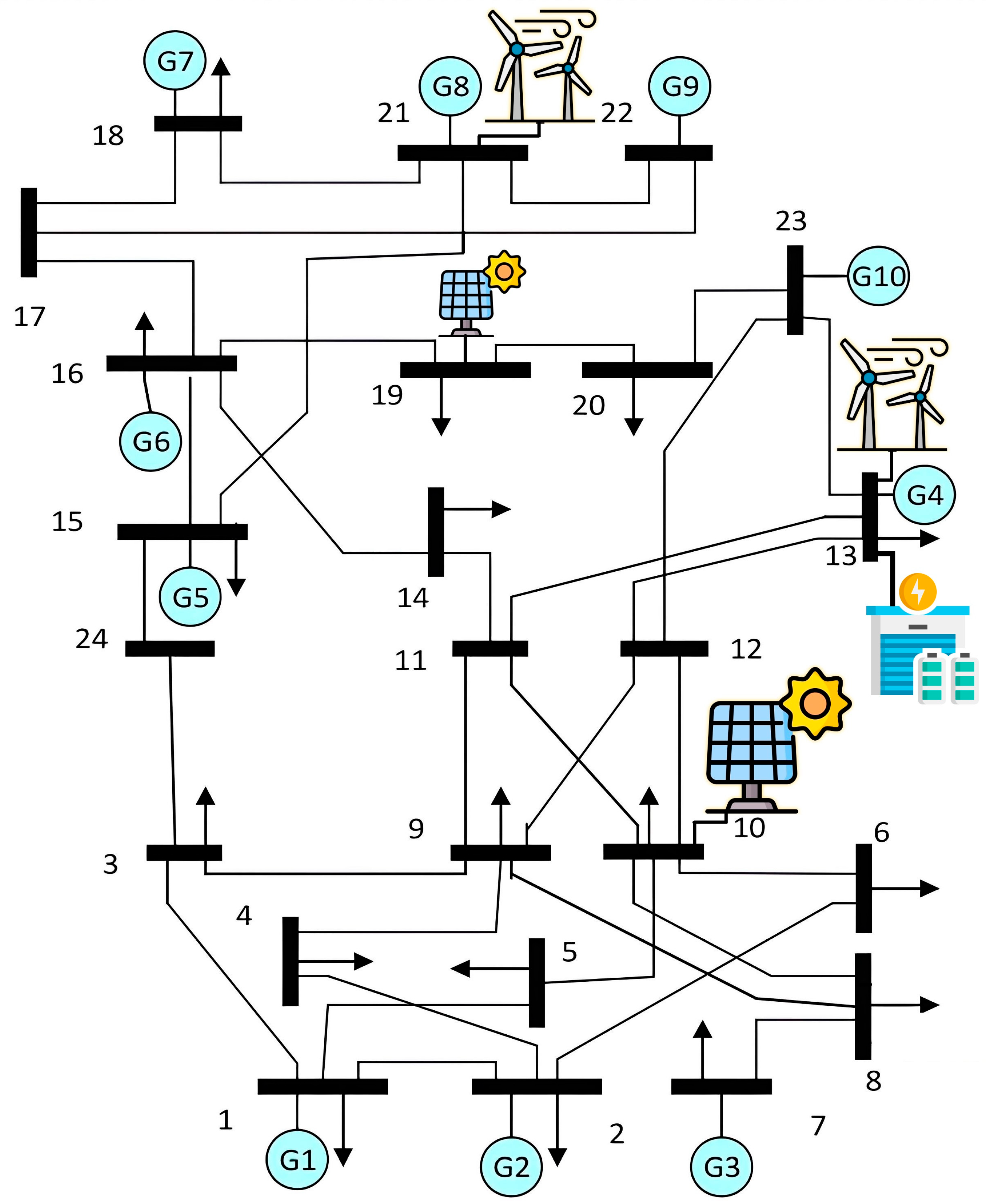
Figure 1. Modified IEEE 24-bus reliability test system. Bus numbers are shown in black, and generator indices (G1–G10) are indicated in blue circles.
Energies 18 05245 g001
Figure 2. Actual vs. Forecasted PV Generation Profiles at Bus 10 and Bus 19 on Representative Days (1 February, 1 July, and 1 December 2024).
Energies 18 05245 g002
Figure 3. Actual vs. Forecasted Wind Generation Profiles at Bus 13 and Bus 21 on Representative Days (1 January, 1 July, and 1 December 2024).
Energies 18 05245 g003
Figure 4. Actual vs. Forecasted Demand Profiles at Bus 1 and Bus 8 on Representative Days (1 January, 1 July, and 1 December 2024).
Energies 18 05245 g004
Figure 5. Data-Driven Uncertainty Bounds on Total PV and Wind Generation Profiles for Representative Days in 2024.
Energies 18 05245 g005
Figure 6. Data-Driven Uncertainty Bounds on Total Demand Profiles for Representative Days in 2024.
Energies 18 05245 g006
Figure 7. Daily Battery State-of-Charge and Power Schedule under DDRO-OPF (1 January, 1 April, 1 July & 1 December 2024).
Energies 18 05245 g007
Figure 8. Representative Daily Generator Dispatch Profiles under DDRO-OPF (1 January, 1 April, 1 July & 1 December 2024).
Energies 18 05245 g008
Table 1. Focused Comparison of Literature on Optimal Power Flow in Transmission Systems Under Uncertainty.
Ref.MethodologyUncertainty ModelSystem/ApplicationConstraints & FocusApproach
[44]Multi-stage DROWasserstein Ambiguity SetTransmission & Distribution SystemsRisk (CVaR), Reserve Policies, OPF Control PoliciesModeling of historical forecast errors
[33]DROData-driven Ambiguity SetTransmission System (IEEE 118)Energy-Reserve-Storage Co-dispatchBased on historical data
[47]DDRO-Chance constraintData-driven Uncertainty ModelGeneral Power SystemEconomic Dispatch, ReliabilityModeling variation ranges and distributions
[34]DDROScenario ClusteringTransmission System (IEEE 30, 118)UC, Spatial CorrelationsData-driven scenario clustering
[48]DDROWasserstein MetricReal-Time Economic DispatchAutomatic Generation Control, Frequency Regulation ConstraintsCopula-based modeling of correlated signals
[45]DROImproved Wasserstein MetricTransmission System (IEEE 118)Optimal Dispatch, Electric vehicles UncertaintyBased on extreme scenarios for efficiency
[35]MetaheuristicN/ATransmission System (IEEE 30)OPF (Fuel cost, loss, voltage deviation)Deep Reinforcement Learning Algorithm
[49]Probabilistic AnalysisProbabilistic DistributionsTransmission System (IEEE 30)Probabilistic OPFN/A
[36]MetaheuristicN/ATransmission System (IEEE 30, 118)Probabilistic OPFEvolutionary Whale Optimization Algorithm
[37]MetaheuristicStochastic OPFTransmission System (IEEE 30)Stochastic OPF, Reserve/Penalty CostsDiscrete Multi-Objective Algorithm
[50]Stochastic SimulationMonte CarloTransmission System (30, 57, 118)OPF, Modeling variable correlationsN/A
[51]Stochastic OPFScenario-basedTransmission GridOPF, Reserve Management, Curtailment MinimizationGaussian Distribution Forecasting Model for advanced forecasting
[43]Stochastic Tri-levelEpistemic Uncertainty (Failures)Transmission System (IEEE 24, 118)Reliability, Cascading Failures, Criticality AnalysisN/A
[39] Distributed OptimizationDeterministicIntegrated Trans.-Dist. SystemAC OPF, Scalability‘aladin’ Algorithm
Note: “N/A” indicates that the aspect is not applicable to the methodology or not explicitly reported in the referenced work.
Table 2. Line Parameters of the Modified IEEE 24-Bus System.
From BusTo Busr (p.u.)x (p.u.)b (p.u.)Limit (MW)
120.00260.01390.4611175
130.05460.21120.0572175
150.02180.08450.0229175
240.03280.12670.0343175
260.04970.1920.052175
390.03080.1190.0322175
3240.00230.08390.0400
490.02680.10370.0281175
5100.02280.08830.0239175
6100.01390.06052.459175
780.01590.06140.0166175
890.04270.16510.0447175
8100.04270.16510.0447175
9110.00230.08390.0400
9120.00230.08390.0400
10110.00230.08390.0400
10120.00230.08390.0400
11130.00610.04760.0999500
11140.00540.04180.0879500
12130.00610.04760.0999500
12230.01240.09660.203500
13230.01110.08650.1818500
14160.00500.03890.0818500
15160.00220.01730.0364500
15210.003150.02450.2061000
15240.00670.05190.1091500
16170.00330.02590.0545500
16190.00300.02310.0485500
17180.00180.01440.0303500
17220.01350.10530.2212500
18210.001650.012950.1091000
19200.002550.01980.16661000
20230.00140.01080.0911000
21220.00870.06780.1424500
Table 3. Generator Parameters of the Modified IEEE 24-Bus System.
GenPmax (MW)Pmin (MW)RampUp (MW/h)RampDown (MW/h)MinUp (h)MinDown (h)b ($/MWh)c ($)CostsD ($)Costst ($)cp (Bus)
g14001005050325.4754.70018
g24001005050325.4754.70021
g315230.430303213.32133.21430.41430.41
g415230.430303213.32133.21430.41430.42
g515554.2525253216160015
g615554.2525253210.52105.231231216
g7310108.540403210.52105.262462423
g835014040403210.89108.92298229823
g93507520203220.7207172517257
g10350206.8520203220.93209.33056.73056.713
g11601210103226.11261.143743715
g123000151532000022
Table 4. Forecasting Metrics for Renewables and Demands.
Resource/DemandValidation MAE (MW)Validation RMSE (MW)Test MAE (MW)Test RMSE (MW)
Bus 13 Wind7.83812.9757.99813.315
Bus 21 Wind7.36411.9467.68812.714
Bus 10 PV6.38114.9116.00214.098
Bus 19 PV4.0979.5543.9709.411
Demand Bus 10.8791.3650.8401.258
Demand Bus 20.5440.8900.5851.030
Demand Bus 31.3341.8421.3541.935
Demand Bus 40.4420.7090.4700.814
Demand Bus 50.4050.6000.4930.795
Demand Bus 60.8051.3020.8401.370
Demand Bus 70.8361.3330.8701.374
Demand Bus 80.7601.3370.7951.353
Demand Bus 90.9961.5171.1051.847
Demand Bus 101.1351.7311.2261.972
Demand Bus 131.6722.7462.2514.092
Demand Bus 141.4362.4241.4442.342
Demand Bus 151.7122.6241.8502.987
Demand Bus 160.8321.3560.8441.292
Demand Bus 183.3634.6403.7946.252
Demand Bus 191.1471.7611.1591.750
Demand Bus 200.7781.2430.8321.307
Table 5. Integrated Relative Forecasting Metrics.
Resource/DemandCapacity/Mean (MW)MAE (MW)MAE %RMSE (MW)RMSE %
Bus 13 Wind1508.05.313.38.9
Bus 21 Wind1507.75.112.78.5
Bus 10 PV2006.03.014.17.1
Bus 19 PV1004.04.09.49.4
Demand Bus 1750.81.11.31.7
Demand Bus 2970.60.61.01.0
Demand Bus 31801.40.81.91.1
Demand Bus 4740.50.70.81.1
Demand Bus 5710.50.70.81.1
Demand Bus 61360.80.61.41.0
Demand Bus 71250.90.71.41.1
Demand Bus 81710.80.51.40.8
Demand Bus 91751.10.61.81.0
Demand Bus 101951.20.62.01.0
Demand Bus 132652.30.94.11.5
Demand Bus 141941.40.72.31.2
Demand Bus 153171.90.63.00.9
Demand Bus 161000.80.81.31.3
Demand Bus 181603.82.46.33.9
Demand Bus 191811.20.71.81.0
Demand Bus 201280.80.61.31.0
Table 6. Hourly Delta Statistics (MW).
ResourceMin DeltaMax DeltaAvg. DeltaStd. Dev.
Bus 13 Wind12.0670.5717.8913.45
Bus 21 Wind9.9065.3016.2012.10
Bus 10 PV0.0545.2010.309.80
Bus 19 PV0.0522.105.604.90
Demands (Avg.)0.744.701.820.62
Table 7. Summary of Daily Optimization Metrics.
Date 2024Total Cost ($)DG Generation (MW)Renewable Actual (MW)Renewable Forecast (MW)Renewable Diff. (MW)Demand Actual (MW)Demand Forecast (MW)Demand Diff. (MW)Renew. Exceedance (%)Demand Exceedance (%)
1 January280,55128,00428283042−21428,44228,509−662.020.5
1 February284,43628,39247984813−1530,85730,66918817.77.6
1 March292,83429,2325025485117431,64331,5469710.411.7
1 April267,90826,7397315718712831,65831,3892689.311.0
1 May279,50627,8997465723223332,84032,59524610.422.3
1 June299,92729,94134183491−7330,90830,8951313.523.7
1 July253,12925,26167396758−1929,31929,483−16425.019.1
1 August273,62827,31158496115−26730,87830,890−1214.513.2
1 September300,51430,00033183463−14630,90630,927−2121.814.9
1 October272,32727,1815893576812530,48930,4127718.712.9
1 November274,82527,43154735506−3330,50530,40110420.816.4
1 December289,35428,8843926378314330,10230,130−2915.622.3
Table 8. Benchmark comparison of cost and reliability across deterministic, stochastic, Γ-robust, and DDRO models.
MethodAvg. Daily Cost (USD)Avg. Renewable Exceedance (%)Avg. Demand Exceedance (%)Remarks
Deterministic265,00022.020.5Lowest cost, poor reliability
Stochastic278,00017.016.8Moderate improvement
Γ-Robust305,00011.511.0Reliable but costly
Proposed DDRO289,00014.815.9Balanced trade-off
Table 9. Sensitivity of DDRO results to Wasserstein radius (ε) and cost-scaling parameter ( η c ).
ε η c Avg. Daily Cost (USD)Renew. Exceedance (%)Demand Exceedance (%)Avg. Runtime (min)Remarks
0.50.05276,00019.820.23.1Optimistic, low cost, low reliability
1.00.05289,00014.815.93.4Balanced
2.00.05304,00011.612.23.7Very conservative, costly
1.00.02285,00017.918.23.2Smaller η c weakens robustness
1.00.10295,00013.213.73.8Larger η c enforces stricter protection
Table 10. Sensitivity of DDRO results to different percentile bounds for renewable and demand uncertainty.
Percentile BoundsAvg. Daily Cost (USD)Renew. Exceedance (%)Demand Exceedance (%)Remarks
10th–90th277,00019.619.2Narrow bounds: lower cost, weaker protection
5th–95th289,00014.815.9Balanced trade-off
2.5th–97.5th296,00013.413.7Wide bounds: higher cost, stronger protection
Table 11. Summary of daily solution times for the DDRO model on the 24-bus system.
Date (2024)Solution Time (s)Date (2024)Solution Time (s)
1 January871 July126
1 February911 August96
1 March1031 September118
1 April851 October92
1 May1121 November101
1 June1291 December108
Disclaimer/Publisher’s Note: The statements, opinions and data contained in all publications are solely those of the individual author(s) and contributor(s) and not of MDPI and/or the editor(s). MDPI and/or the editor(s) disclaim responsibility for any injury to people or property resulting from any ideas, methods, instructions or products referred to in the content.