Article

Optimization Method for Regulating Resource Capacity Allocation in Power Grids with High Penetration of Renewable Energy Based on Seq2Seq Transformer

1
State Grid Corporation of China, Central China Branch, Wuhan 430077, China
2
School of Electrical Engineering and Automation, Wuhan University, Wuhan 430072, China
3
Economic and Technological Research Institute, State Grid Hubei Electric Power Company, Wuhan 430077, China
4
School of Law, Wuhan University, Wuhan 430072, China
*
Author to whom correspondence should be addressed.
Energies 2025, 18(19), 5218; https://doi.org/10.3390/en18195218
Submission received: 23 August 2025 / Revised: 15 September 2025 / Accepted: 16 September 2025 / Published: 1 October 2025
(This article belongs to the Special Issue Advancements in Power Electronics for Power System Applications)

Abstract

With the high penetration of renewable energy integrated into the power grid, the system exhibits strong randomness and volatility. To balance these uncertainties, a large amount of flexible regulating resources is required. This paper proposes an optimization method based on a Seq2Seq Transformer model, which takes stochastic renewable energy and load data as inputs and outputs the allocation ratios of various regulating resources. The method considers renewable energy stochasticity, power flow constraints, and adjustment characteristics of different regulating resources, while constructing a multi-objective loss function that integrates ramping response matching and cost minimization for comprehensive optimization. Furthermore, a multi-feature perception attention mechanism for stochastic renewable energy is introduced, enabling better coordination among resources and improved ramping speed adaptation during both model training and result generation. A multi-solution optimization framework with Pareto-optimal filtering is designed, where the Decoder outputs multiple sets of diverse and balanced allocation ratio combinations. Simulation studies based on a regional power grid demonstrate that the proposed method effectively addresses the problem of regulating resource capacity optimization in new-type power systems.

1. Introduction

With the continuous advancement of the “dual-carbon” strategy, the share of renewable energy in China’s power system has been steadily increasing. The installed capacity of renewables such as wind and photovoltaic (PV) power has grown rapidly, gradually replacing traditional thermal power and becoming the dominant type of generation. By the end of 2024, China’s total installed renewable capacity had exceeded 1.4 billion kW, accounting for more than 50%. However, renewable resources are characterized by significant randomness, volatility, and reverse peak-shaving capability, with their output strongly influenced by factors such as weather and seasonal variations. As the penetration of renewable energy continues to rise, the power system faces severe challenges in terms of source-load balance, operational scheduling, and ancillary services [1,2,3].
Traditional countermeasures have mainly focused on enhancing the carrying capacity of the power grid, such as strengthening backbone network structures, building cross-regional transmission channels, and improving grid automation. However, against the high-penetration renewable background, simply relying on transmission expansion and grid reinforcement is no longer sufficient to fully address the peak-valley gap caused by renewable uncertainty [4,5]. Therefore, it is urgent to establish an operational support system tailored to future power systems, in which the planning and optimal scheduling of flexible and dispatchable resources play a central and critical role.
Flexible regulating resources mainly include: traditional dispatchable units (such as conventional thermal power, hydropower, and gas turbines), new energy storage technologies (including battery energy storage, pumped storage, and compressed air energy storage), and “controllable load” resources such as interruptible loads, virtual power plants, and demand response. These resources not only possess fast response and short-cycle regulation capabilities, but can also participate in medium- and long-term ancillary services, supporting system frequency and voltage control, thereby acting as a “stabilizer” against fluctuations in renewable energy output under high penetration conditions [6].
The optimal allocation of dispatchable resources involves several key factors: their regulation capabilities (ramp rate, minimum output, start-up/shutdown time); their operational economics (unit regulation cost, service life, depreciation, and operation and maintenance costs); and their complementary characteristics with renewable energy output in terms of time, space, and resource attributes.
At present, research on the optimal allocation of flexible regulating resources against the high-penetration renewable energy background both domestically and internationally mainly focuses on the following directions.
For system-level resource coordination and allocation models, institutions such as NREL and EPRI in the United States have proposed “whole-system flexibility assessment frameworks,” which integrate flexible resources into system planning models and establish multi-temporal and multi-spatial coordinated scheduling mechanisms spanning from the supply side to the demand side [7,8,9]. For example, multi-objective allocation models based on chronological simulation and scenario analysis are able to simultaneously evaluate the reliability, economic efficiency, and flexibility redundancy of resource allocation. In addition, in the area of integrated “generation-grid-load-storage” planning, extensive studies have been conducted. Typical approaches include multi-energy coupling optimization models, hierarchical and zonal resource allocation frameworks, and storage system economic evaluation models, all of which aim to address the problem of robust system configuration under renewable output fluctuations [10,11,12,13].
For complementarity models between regulating resources and renewable energy, renewable output modeling frequently adopts probabilistic scenario generation methods, Monte Carlo simulations, and Copula-based wind-solar joint distribution models to achieve probabilistic forecasting and risk assessment of renewable generation. Furthermore, dimension reduction and clustering techniques for renewable scenarios, such as K-means and deep learning methods, have been developed to improve the computational efficiency of planning and allocation models [14,15,16]. In addition, by leveraging the complementarities between renewables and energy storage, various models have been developed, including “wind-solar-storage + load” typical day models, “virtual power plant coordination” models, and “time-coupled constraint configuration models,” which provide methodological support for the coordinated optimization of multiple flexible resources [17].
In terms of economic dispatch and optimization algorithms, the economic modeling of flexible resources is commonly formulated using mixed-integer programming (MIP), dynamic programming (DP), genetic algorithms (GA), particle swarm optimization (PSO), and other system optimization approaches [18,19]. Multi-round simulation tests conducted by institutions such as NREL and MIT have demonstrated that joint regulation by energy storage and fast-response gas turbines can effectively reduce system reserve requirements and scheduling costs. Advanced modeling techniques including game theory, Stackelberg games, Nash equilibrium, and reinforcement learning have also been introduced to establish collaborative decision-making mechanisms among multiple stakeholders (e.g., grid operators, power producers, and storage providers), balancing dispatch objectives with multi-party economic incentives. In multi-source integration scenarios, joint configuration optimization methods have become a major research focus [20,21,22].
So the key to operating future power systems lies in achieving coordinated cooperation among heterogeneous resources, optimizing allocation under economic drivers, and ensuring system reliability. In the face of renewable energy uncertainty, constructing a flexible resource allocation framework with adaptive regulation capabilities is an essential means of promoting the planning and scheduling of new-type power systems.

2. Problem Modeling

The optimal allocation of flexible regulating resources required for stable and economic operation of power systems with high renewable penetration is essentially a multi-objective optimization problem characterized by cross-temporal-spatial interactions, stochastic dynamics, and strong coupling. Wind, solar, and load all exhibit stochastic fluctuations with strong temporal and spatial correlations. Meanwhile, flexible regulating resources (such as deep peak-shaving thermal units, pumped storage, and battery storage) introduce inter-temporal constraints, including minimum on/off times, ramping limits, reservoir level coupling, and battery degradation. On the grid side, power flow balance, stability, and dynamic constraints must also be satisfied simultaneously. The core of the planning problem lies in combinatorial optimization—that is, determining the optimal capacity mix of deep-regulating thermal power, pumped storage, and battery storage under multiple scenarios, while ensuring ramping speed compatibility among different types of power sources.
In this study, fundamental power sources and base loads in the grid are not considered. Instead, the focus is placed on renewable energy and corresponding load integration. Both renewable generation and load vary stochastically, making natural source-load balance impossible; only with the participation of flexible regulating resources can balance be achieved.

2.1. System Power Difference Model

The first step is to characterize the uncertainties of stochastic renewable energy and load, including typical daily power scenarios of wind, solar, and load, multi-scenario clustering, and chance-constrained sets. Within the scheduling horizon (e.g., one day divided into 15 min intervals, resulting in T = 96 time steps), the power difference between renewable generation and load is defined, from which the required regulating resource power can be derived.
P bal ( t ) = k = 1 N l P load ( k ) ( t ) i = 1 N w P wind ( i ) ( t ) j = 1 N p P pv ( j ) ( t )
P bal ( t ) : Regulating resource power;
P load ( k ) ( t ) : Power of the k-th load;
P wind ( i ) ( t ) : Power of the i-th wind unit;
P pv ( j ) ( t ) : Power of the j-th photovoltaic unit;
The above includes power forecasts of Nw wind units, Np photovoltaic units, and Nl load nodes. The power difference between loads and renewable generation must be compensated by flexible regulating resources. In this paper, three types of flexible resources are mainly considered: deep peak-shaving thermal power units, pumped storage, and battery energy storage. These three categories differ in response speed and economic cost, as well as in their application scenarios within the power grid.

2.2. Proportional Allocation of Flexible Resources

Different types of flexible regulating resources vary in cost and response speed, and their deployment within the power grid depends on specific application scenarios. To cope with the stochastic fluctuations of multi-point renewable generation, multiple regulating resources must be analyzed under cross-temporal-spatial coupling and total cost optimization. For instance, deep peak-shaving thermal units are subject to nonlinear thermodynamic boundaries and ramping/minimum output constraints; pumped storage requires piecewise linearization of reservoir level and waterway curves; and battery energy storage involves degradation and lifetime costs. For the sake of analytical convenience, the three types of regulating resources are normalized, with the proportions of each type summing to 1.
x ( t ) = [ x coal ( t ) , x hydro ( t ) , x battery ( t ) ] , x i ( t ) [ 0 , 1 ] , i = 1 3 x i ( t ) = 1
x coal ( t ) , x hydro ( t ) , x battery ( t ) : proportions of the three types of flexible regulating resources in the final calculation results.
P i ( t ) = x i ( t ) · P bal ( t )

2.3. Multi-Objective Loss Function Design

The optimization of heterogeneous multi-source resource coordination is driven by both economic efficiency and system reliability. The loss function is formulated as a weighted combination of two components: a ramping-matching term and a cost term.
Ramping-matching loss:
L ramp = t = 2 T i = 1 3 Δ P i ( t ) x i ( t ) · Δ P bal ( t )
Δ P i ( t ) = P i ( t ) P i ( t 1 )
Operational cost loss:
L cost = t = 2 T i = 1 3 c i · x i ( t ) · P bal ( t )
L total = λ 1 · L ramp + λ 2 · L cost
Here, λ1 and λ2 are weighting coefficients, determined according to the trade-off between system response and cost requirements.
Finally, at the power system level, steady-state power flow and stability constraints are incorporated into the overall verification process, thereby forming a closed-loop framework of “capacity combination–temporal coordination of power variation–risk assessment.” By unifying capacity reserves, ramping speed, and cost analysis into a consistent risk metric, the approach achieves a balance between stability and economic optimality under uncertainty.

3. Seq2Seq Transformer Model Structure Design

3.1. Seq2Seq Transformer Architecture

In traditional time-series modeling, recurrent neural networks (RNNs) and their variants (such as LSTM and GRU) have been widely applied to wind power, photovoltaic, and load forecasting as well as combined analysis. However, these models suffer from two major limitations:
Information transmission bottleneck: Since information is propagated along the temporal dimension, the efficiency of modeling long-range dependencies is relatively low;
Low training efficiency: Sequential processing prevents effective parallelization, thereby limiting training acceleration and hardware utilization.
In this study, the Seq2Seq Transformer model adopts a standard Encoder–Decoder Transformer architecture. The Encoder is responsible for modeling the temporal features of stochastic wind and photovoltaic inputs, while the Decoder progressively generates the output sequences representing the proportions of the three types of flexible resources. Each Transformer module consists of multi-layer attention mechanisms and feed-forward networks, providing strong capabilities for time-series feature extraction and nonlinear representation. The architecture includes the following components:
Encoder: Performs multi-layer multi-head self-attention operations on the multi-source inputs over the future T steps, extracting global temporal features of renewable energy and load.
Decoder: At each step, takes as input either the proportion generated in the previous step (or zero initialization) and generates the regulating resource proportions through Masked Self-Attention combined with cross-attention mechanisms.
Output Head: A linear mapping followed by a Softmax operation, ensuring that the sum of the proportions of all flexible resources equals 1 at each time step.
With its parallelized computation, multi-head attention mechanism, and residual connections, the Transformer model overcomes the aforementioned limitations and is particularly well-suited for modeling high-dimensional, multi-source inputs in new-type power system planning and scheduling. Therefore, this study introduces the Transformer into the planning problem of power systems with high renewable penetration, aiming to achieve time-series modeling of multiple stochastic variables from wind and solar generation, dynamic prediction and analysis of balancing and coordination strategies between renewables and flexible resources across multiple time periods, and the generation of proportion sequences of flexible resources at each time step.
The Seq2Seq Transformer demonstrates superior accuracy, flexibility, and practicality in forecasting renewable energy power output and load. Compared to RNN, LSTM, GRU, and TCN, it offers distinct advantages in handling stochastic time series from wind, solar, and load sources, including parallel computation, effective long-range dependency modeling, cross-variable interaction flexibility, and interpretability. The attention mechanism stands as its core innovation, enabling the model to uncover complex temporal and multi-source data correlations more precisely, thereby significantly enhancing forecasting accuracy and real-world applicability.

3.2. Positional Encoding

Positional encoding is employed to explicitly represent the temporal order of the input sequence. Each input is first linearly projected into a d_model-dimensional space before being passed into the Transformer module.
For each input sequence X ( t ) T × d input , a linear layer is applied to embed it into the d_model-dimensional space required by the Transformer:
X ^ ( t ) = X ( t ) · W emb + b
Considering that the Transformer itself does not possess inherent sequence awareness, positional encoding is introduced to preserve temporal order.

3.3. Encoder Structure

The Encoder consists of Ne stacked sub-layers, each comprising:
  • Multi-Head Self-Attention;
  • Residual Connection;
  • Position-wise Feed-Forward Network;
  • Layer Normalization (LayerNorm).
At each time step of the input sequence, dependencies with other time steps are established through the attention mechanism, effectively capturing the structural relationships between long-term load and renewable energy fluctuations. The attention mechanism is formulated in the form of scaled dot-product attention:
Attention ( Q , K , V ) = softmax Q K d k V

3.4. Decoder Structure

The Decoder also consists of Nd stacked layers, each containing three sub-modules:
(1)
Masked Multi-Head Attention: prevents information leakage from future time steps;
(2)
Encoder–Decoder Cross Attention: captures dependencies between the Encoder outputs and the current decoding state;
(3)
Feed-Forward Network with Residual Connection: the outputs are mapped to grid power flow calculations to check whether actual constraints are satisfied, with the residuals representing power flow deviations.
At each time step, the output proportion is determined jointly by the decoded results from previous time steps and the overall input prediction sequence. This structure enables the Decoder to integrate both historical outputs and global system information, thereby achieving causal decoding.
The input to the Decoder can be initialized with zeros; during training, the initial values are constructed using a sliding window of historical outputs, i.e., the outputs from the previous iteration.

3.5. Output Layer and Constraint Handling

The final output of the Decoder is passed through a fully connected linear mapping layer to obtain the raw proportion vector of flexible regulating resources:
z t = Linear ( h t ) 3
Each element in the vector represents the required capacity of a specific regulating resource. During training, a large number of such values are generated. To ensure that the sum of proportions equals 1, these values are processed through the Softmax function:
x ( t ) = softmax ( z t )
Thus, the proportion of each regulating resource lies within [0, 1] [0, 1] [0, 1] and satisfies
i = 1 3 x i ( t ) = 1
which conforms to the power allocation constraints of source–load balance in power system operation.

4. Input Data Generation and Attention Mechanism

4.1. Input Data Generation

Wind power, photovoltaic, and load exhibit strong stochasticity, making accurate forecasting highly challenging. Their behavior can only be approximated by generating multiple sets of wind, solar, and load power curves under different probabilities. The performance of the Transformer model largely depends on the organization of these input data. For the coordinated planning problem of flexible resources, this study adopts the following modeling scheme:
The model input consists of the time-series forecasting results over the next T steps, including:
Power forecasts of Nw wind units;
Power forecasts of Np photovoltaic units;
Demand forecasts of Nl load nodes.
The overall input matrix is defined as:
X ( t ) T × ( N w + N p + N l )
Based on the probabilistic models of renewable energy and load fluctuations, a large number of renewable and load scenarios can be generated using historical and forecast data, with each scenario representing a possible power curve. However, probabilistic models often produce an excessively large number of scenarios, leading to a sharp increase in the scale of optimization calculations. Therefore, it is necessary to reduce the number of scenarios to a small subset of the most representative and probable ones, a process known as scenario reduction.
To this end, the forecast bin method is employed to characterize the error distribution of point forecasts. Specifically, forecast values are first sorted in descending order and divided into several numerical intervals. Then, according to the magnitude of the forecast value, the corresponding data pairs [forecast, observation] are assigned to the corresponding interval. With the interval length predefined, the set of data within each interval constitutes a “forecast bin.” On this basis, renewable energy and load scenarios can be generated according to their respective probability distributions [23,24].

4.2. Multi-Feature Attention Mechanism for Input Data

The direct variation features of highly stochastic wind, photovoltaic, and load data are not sufficiently distinct. To achieve better performance in Transformer training, multiple features must be extracted to jointly characterize their variability, thereby forming a multi-feature attention mechanism. Specifically, features such as the maximum and minimum values, ramping rates, ramp-up and ramp-down frequencies, and peak-to-valley differences of wind, solar, and load curves are considered as feature quantities for the Transformer attention mechanism.
These feature quantities are explicitly incorporated into the computable formulas of the Transformer’s attention scores and weights. Let Pt ∈ [0, 1] denote the normalized active power output sequence (modeled separately for wind, solar, and load, or jointly as multi-channel inputs), with discrete time steps t = 1, …, T, and step size Δt.
(1)
Definition of Temporal Physical Features
First-order ramping (difference) of the power curve:
r t = P t P t 1 Δ t , t = 2 , , T , r 1 = 0
r t + = max ( r t , 0 ) ,   r t = max ( r t , 0 )
Sliding-Window Extremes and Peak–Valley Difference of Input Data (Window W)
P t max = max τ [ t W + 1 , t ] P τ ,   P t min = min τ [ t W + 1 , t ] P τ ,   Δ t = P t max P t min
Extrema indicators of the power curve (determined by sign changes in the first-order difference):
σ t p e a k = 1 { r t 1 > 0 , r t 0 } ,   σ t v a l l e y = 1 { r t 1 < 0 , r t 0 }   ( t 2 )
Upward/Downward ramping frequency of the power curve:
υ t + = τ = t W + 1 t { r τ 1 0 , r τ > θ + }
υ t = τ = t W + 1 t { r τ 1 0 , r τ < θ }
Feature vector of the power curve:
ψ t = P t , r t , | r t | , r t + r t , υ t + , υ t , Δ t , σ t peak , σ t valley
Feature ψ ˜ t is obtained by normalizing ψ t .
ψ ˜ t = B N ( ψ t )
Batch Normalization (BN) is used as the activation function.
(2)
Feature Embedding and Backbone Representation
The original inputs consist of value embeddings (xt) and positional embeddings (pt). The extracted physical features are linearly projected into the same dimension as the model:
e t = W ψ ψ ˜ t + b ψ d ,   h t = x t + p t + e t d
d: dimension of the model hidden space;
dk: dimension of queries/keys (Q/K);
dv: dimension of values (V);
df: dimension of physical features;
W, b: linear mapping weights and bias from physical features to the model space.
e t denotes the embedded features, while h t represents the hidden states used for the attention mechanism.
(3)
Feature-Aware Attention Scoring
The variation characteristics of photovoltaic, wind, and load curves are evaluated by identifying their features and computing corresponding scores. During Transformer training, the attention mechanism focuses primarily on these feature-aware analyses.
q i = W Q h i , k j = W K h j , v j = W V h j
WQ: learnable projection matrix that maps hidden vectors into the Query space;
WK: learnable projection matrix that maps hidden vectors into the Key space;
WV: learnable projection matrix that maps hidden vectors into the Value space;
qi: Query vector at position i, representing the type of feature pattern to be searched for in renewable and load data;
kj: Key vector at position j, representing the feature patterns currently available;
vj: Value vector at position j, whose features are weighted and aggregated into the final representation.
s i j ( 0 ) = q i k j d k
Let s i j ( 0 ) denote the initial score from position i to position j. On this basis, a feature similarity kernel ( κ ), a physical bias ( b i j ( phys ) ), and a relative distance bias ( b i j ( rel ) ) are incorporated to obtain the total attention score:
s i j = s i j ( 0 ) + κ ( ψ ˜ i , ψ ˜ j ) + b i j ( phys ) + b i j ( rel ) + m i j
Here, mij is the masking term, reflecting causal, local, and block-sparse constraints in the model structure.
κ ( ψ ˜ i , ψ ˜ j ) = α · exp 1 2 ( ψ ˜ i ψ ˜ j ) Λ ( ψ ˜ i ψ ˜ j ) , Λ 0
After computing attention scores for the feature quantities, the attention weights are calculated as follows:
a i j = exp ( s i j ) l N ( i ) exp ( s i l )
where N ( i ) denotes the index set of positions that position i is allowed to attend to
Attn ( i ) = j N ( i ) a i j v j
To further enhance flexibility, various feature quantities are used to modulate the Query/Key vectors through learnable operations, such as additive or multiplicative controls:
q ˜ i = W Q h i + U Q f ˜ i , k ˜ j = W K h j + U K f ˜ j γ i = σ ( w Q f ˜ i ) , γ j = σ ( w K f ˜ j ) , q ^ i = ( 1 + γ i ) q ˜ i , k ^ j = ( 1 + γ j ) k ˜ j s i j = q ^ i k ^ j d k + b i j ( phys ) + b i j ( rel ) + m i j
σ : Sigmoid function.
When all feature and bias coefficients are set to zero, the formulation degenerates to the standard attention mechanism.
In addition to calculating attention scores separately for photovoltaic, wind, and load data, their interrelations must also be considered. Specifically, cross-attention between these three categories (e.g., wind–solar–load multi-point complementarity) is computed. For instance, wind–solar feature complementarity is captured through specialized attention terms.
s i j A B = ( W Q h i ( A ) ) ( W K h j ( B ) ) d k + κ f ˜ i ( A ) , f ˜ j ( B ) + b i j ( phys ) + b i j ( rel ) + m i j
Overall, the above formulation systematically injects feature quantities—such as maximum/minimum values, ramping rates, ramp-up/down frequencies, and peak–valley differences—into four levels of the attention mechanism. This is seamlessly integrated with the standard Transformer, ultimately enabling comprehensive evaluation of photovoltaic, wind, and load data and identification of their characteristic variation parameters.
High-penetration renewable energy data exhibit significant stochasticity and temporal dependency, as power output fluctuates due to changes in factors such as wind speed and solar irradiance. In this study, features such as the maximum and minimum values of wind and solar generation curves, ramp rates, ramp-up and ramp-down frequency, and peak-valley magnitudes are incorporated as attention features in the Transformer model. These elements also reflect and reinforce the modeling of temporal constraints.

5. Pareto-Based Multi-Solution Output Series

5.1. Multi-Objective Analysis of Outputs

The output objective is the proportion combination of the three types of flexible resources at each time step t. However, renewable generation exhibits strong seasonality, meaning that the required regulating resources differ across quarters. To address the stochastic nature of wind and solar generation, multiple candidate solutions must be generated and analyzed.
Each candidate solution consists of a proportion combination of the three types of flexible resources.
x ( t ) = [ x coal ( t ) , x hydro ( t ) , x battery ( t ) ]
For the multi-solution extension, the output dimension is defined as:
Y ^ T × K × 3
In power system planning and operational scheduling scenarios, response speed and economic efficiency are often the two core objectives, yet they are inherently conflicting. Thermal power units provide slow ramping but low cost, energy storage offers fast response but high cost, while pumped storage has relatively slow response but moderate cost. According to system requirements for capacity and ramping speed, the rational allocation of these regulating resources to ensure economic feasibility becomes a key issue.
Therefore, under different grid operating conditions and coordination preferences, the optimal solution is not unique. Moreover, due to the stochastic variations of renewable generation and load, grid operating states are complex and dynamic, typically resulting in multiple non-dominated solutions, i.e., the so-called Pareto-optimal solution set.
Over a daily horizon (t = 1, …, T, with 96 steps per day at 15 min intervals), for each candidate solution k, the following three categories of objectives are calculated:
(1)
Economic Efficiency
The total cost of the three types of regulating resources is defined as:
J cost ( k ) = t c coal P coal ( k ) ( t ) + c hydro P hydro ( k ) ( t ) + c batt P batt ( k ) ( t ) Δ t
P i ( k ) ( t ) = x i ( k ) ( t ) P bal ( t )
where c coal , c hydro , c batt represent the unit cost coefficients of thermal power, pumped storage, and battery storage, respectively.
(2)
Dynamic Coordination
The cumulative ramping power required by regulating resources to respond to the stochastic fluctuations of renewable generation and load is expressed as:
J ramp ( k ) = t = 2 T i { coal , hydro , batt } Δ P i ( k ) ( t ) x i ( k ) ( t ) Δ P bal ( t )
(3)
Supply Reliability
When renewable generation peaks, surplus power may occur. If charging capacity of regulating resources is insufficient, this results in curtailed wind or solar power. Conversely, when renewable generation is low, insufficient discharging capacity leads to a risk of unserved load.
This risk is quantified by the reliability index EENS (Expected Energy Not Served), defined as the expected value of unserved energy across stochastic scenarios s = 1, …, S:
EENS s ( k ) = t max { 0 , P L ( s ) ( t ) P RE ( s ) ( t ) i P i ( k ) ( t ) } Δ t
The critical factor lies in maintaining a balance between the renewable–load power difference and the available capacity of regulating resources:
J rel ( k ) = t ( P RE ( s ) ( t ) + i P i ( k ) ( t ) P L ( s ) ( t ) ) / P L ( s ) ( t )
where P RE ( s ) ( t ) denotes renewable generation power in scenario s.

5.2. Multi-Solution Output Structure Design

In this study, the Transformer output is extended with a multi-channel prediction structure, where the Decoder no longer produces a single proportion sequence but instead generates K candidate combinations of regulating resource proportions. At each time step, the Seq2Seq Transformer outputs K sets of regulating resource proportions. For each candidate k, its performance is comprehensively evaluated across S stochastic scenarios according to system operating requirements in different periods, with respect to objectives J cost ( k ) , J ramp ( k ) , and J rel ( k ) .
From the Pareto front consisting of multiple solutions, M representative schemes are selected to ensure both global coverage and avoidance of clustering redundancy. These selected solutions exhibit diversity and balance, facilitating the identification of an optimal solution suitable for practical application, although not necessarily the global optimum.
Considering the operational requirements of power systems with high renewable penetration—including minimum cost, ramping response, and supply reliability—six representative solutions can be identified:
(1)
Cost Min: The regulating resources achieve the lowest cost, which can meet steady-state operation requirements. However, ramping capability is insufficient under sudden power variations, potentially reducing system reliability.
(2)
Ramp Min: Ensures source–load balance even under significant renewable and load fluctuations, but requires a high proportion of fast-response resources (e.g., battery storage), leading to higher costs.
(3)
Risk Min: Guarantees the highest system stability and user supply reliability, minimizing operational risk. However, it may involve renewable curtailment and under-utilization of regulating resources, thereby increasing costs.
(4)
Cost–Risk Trade-off: Balances regulating resource cost and reliability requirements, with lower ramping speed demands. However, its ability to handle strong renewable fluctuations is limited.
(5)
Cost–Coordination Trade-off: Balances regulating resource cost and ramping response requirements. However, curtailment of highly volatile renewable generation may occur, reducing economic efficiency.
(6)
Cost–Coordination–Risk Trade-off: A comprehensive optimization considering all three objectives simultaneously. This represents the most ideal outcome but is difficult to achieve in practice.

6. Case Study

6.1. Case Introduction

For a regional power grid, in addition to the fundamental power sources and base loads, two photovoltaic plants and three wind farms are integrated, along with load demand. The installed capacities are listed in Table 1. The load level is set to the average demand, while the regulating resources include deep peak-shaving thermal units, pumped storage, and battery energy storage. The case study mainly analyzes the supply–demand balance between renewable energy and load, as well as the type and proportion of regulating resources required.

6.2. Model Parameter Settings

The main parameter settings of the Transformer model are shown in Table 2. These parameters directly determine the model’s fitting ability and generalization capability. In this case study, the regional power grid is relatively small, with only a few integrated renewable energy nodes; therefore, the parameter values are set to relatively small scales. For large-scale power grids with more renewable nodes, higher volatility, and complex load profiles, the model dimension d_model and the number of layers can be appropriately increased. Conversely, in scenarios with fewer samples or higher risk, model complexity should be reduced while enhancing regularization measures.
The parameter d_model controls the dimensionality of the input and output feature vectors. In this study, only four feature quantities are considered for renewable and load curves. A higher dimensionality allows the model representation to better approximate reality and achieve higher accuracy, but at the expense of increased training and inference cost. In this study, four feature variables are considered for both renewable energy and load curves. The nhead parameter determines the number of heads in multi-head attention. Typically, more heads lead to better performance. In this case, each group of renewable energy and load curves is independently generated with different probability distributions, showing weak interdependencies. As a result, variations in the four features within one category have limited influence on features in other categories.
The parameter num_layers denotes the number of structural layers in the Transformer model. Increasing the number of layers enhances the model’s ability to capture complex system structures that evolve over time, which is suitable for scenarios with frequent wind and solar fluctuations. A reasonable dropout value helps prevent overfitting in cases of limited samples or excessively large models.

6.3. Results

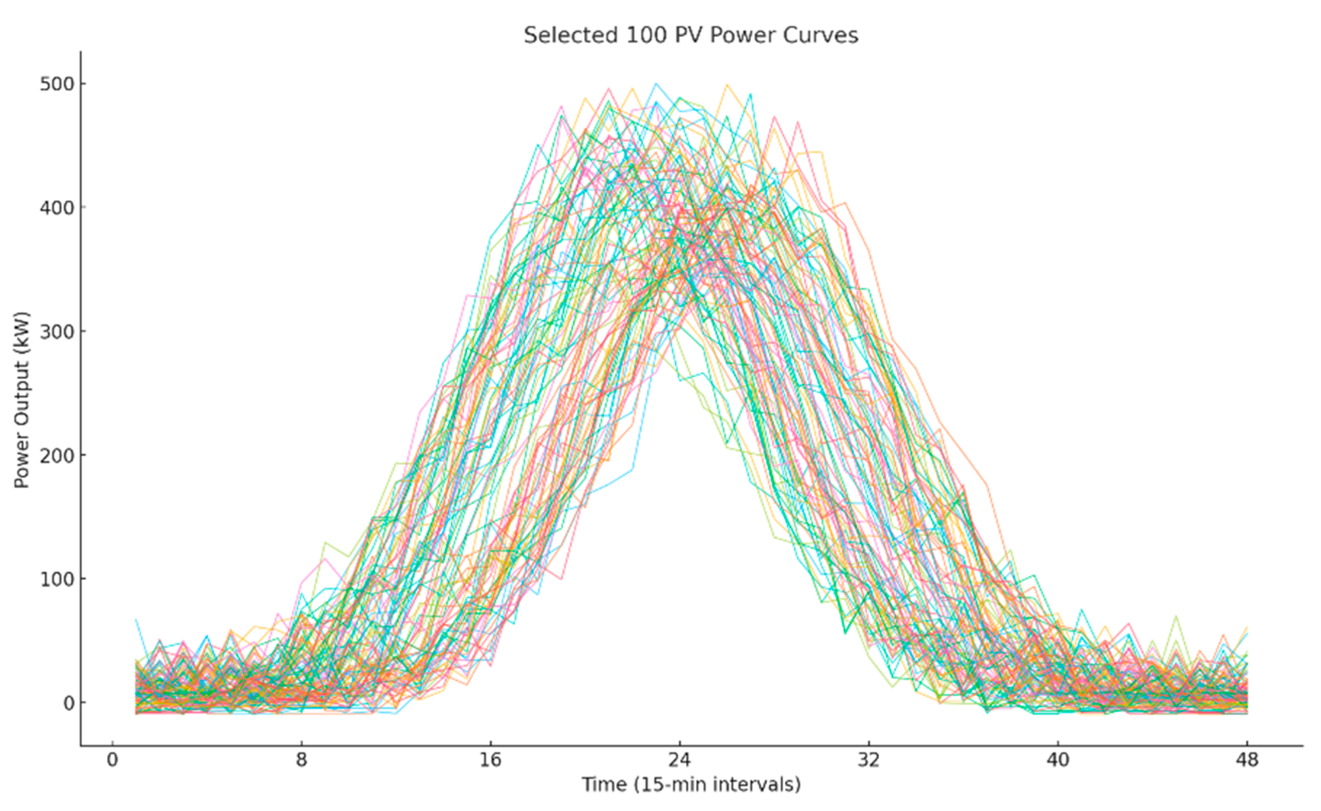
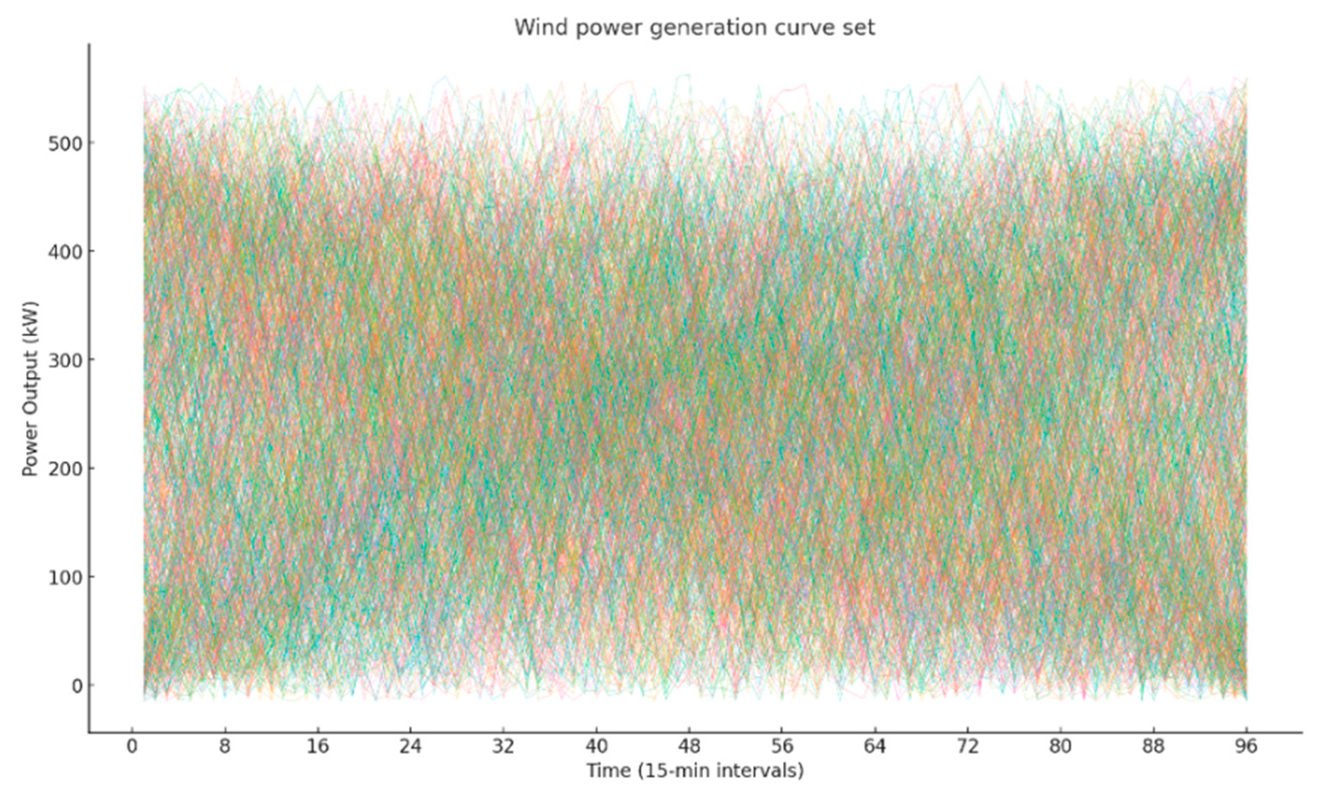
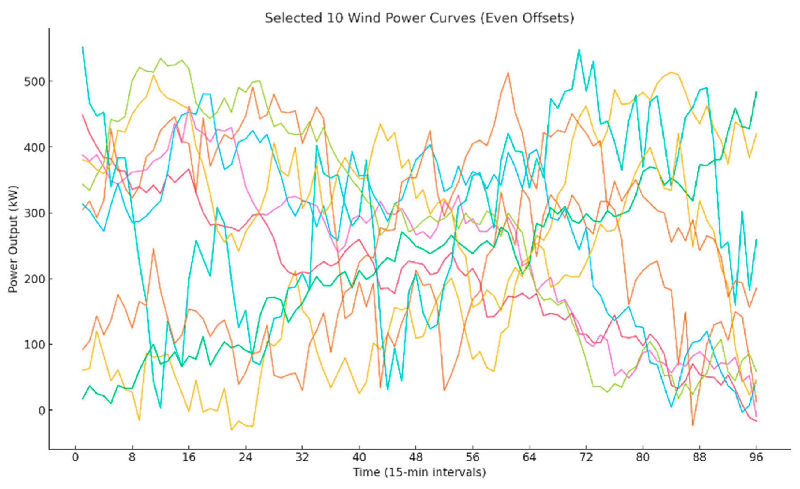
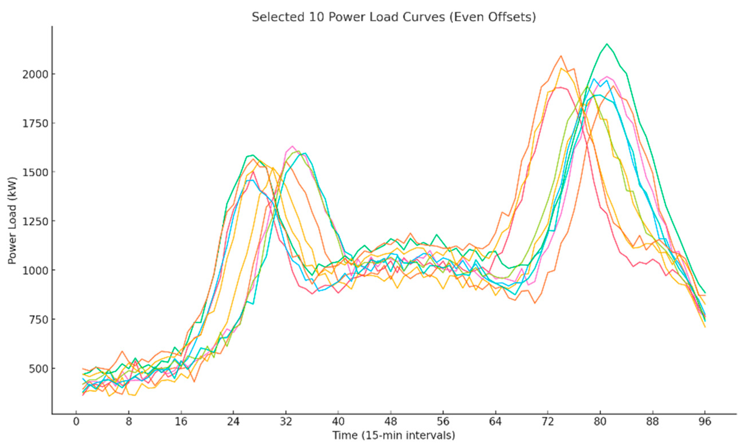
For each renewable and load node, a large number of scenarios are generated. Based on the probability of occurrence of each scenario and the principle of uniform distribution, scenario reduction is performed: first reduced to 1000 scenarios, then to 100 scenarios, and finally to 10 scenarios. These reduced scenarios are used as the inputs to the Seq2Seq Transformer. It should be noted that photovoltaic generation is available only during daytime, yielding 48 time steps per day (15 min per step), whereas wind and load profiles span 96 time steps.
As an example, the scenario analysis of PV station A is presented, while analyses for other PV stations follow a similar approach. Figure 1, Figure 2 and Figure 3 show the reduced photovoltaic scenarios with 1000, 100, and 10 representative cases, respectively.
As another example, the scenario analysis of wind farm C is presented; analyses for other wind farms follow a similar procedure. Figure 4, Figure 5 and Figure 6 illustrate the reduced wind power scenarios with 1000, 100, and 10 representative cases, respectively.
The scenario analysis for load nodes is also similar. Figure 7, Figure 8 and Figure 9 show the reduced load demand scenarios with 1000, 100, and 10 representative cases, respectively.
The three sets of scenarios (1000, 100, and 10) are used as inputs to the Seq2Seq Transformer model for training, generating a large number of results that constitute a solution set. Each regulating resource allocation scheme in the solution set differs across the three objective dimensions, with distinct advantages and disadvantages. This provides planners with diverse and balanced options for decision-making.
By applying the Pareto solution set filtering method, the solution set is further optimized. Based on the proportions of the three types of regulating resources, and considering objectives such as cost minimization, ramping speed minimization, and supply reliability, a series of diverse and balanced solution sets is obtained. The results of the Pareto-filtered outputs corresponding to the three input scenarios are presented in Table 3, Table 4 and Table 5.
The above tables present the final sets of solutions, i.e., the proportion of each regulating resource together with the corresponding values of the three objectives. These solutions satisfy different optimization goals: some achieve the lowest economic cost but have weaker ramping capability; others exhibit good ramping performance and higher supply reliability, but at the expense of higher regulating resource costs. Therefore, no single solution can simultaneously satisfy all three objectives, and the final choice must be made according to practical goals and requirements.
Overall, the size of the training dataset has a significant impact on the stability of the results. In Table 3, with a larger number of training scenarios, the generated results are relatively stable. In Table 4, with fewer training scenarios, the balance of results is somewhat weaker compared to Table 3. In Table 5, with the least training scenarios, the results exhibit stronger fluctuations.
From the perspective of economic efficiency, the lowest-cost solutions are found in Group 2 of Table 3, Group 6 of Table 4, and Group 6 of Table 5. Economic performance is mainly determined by the proportion of battery storage, since batteries currently have the highest unit cost. A proportion of battery storage that is too low will directly affect ramping response matching. Across the three input cases, although the scenario inputs differ significantly, the differences in economic performance are relatively small, as economic efficiency is primarily influenced by the maximum and minimum values of system requirements.
From the perspective of ramping response of regulating resources, the lowest objective values are found in Group 4 of Table 3, Group 4 of Table 4, and Group 5 of Table 5. The ramping performance is directly related to the response speed of regulating resources, as well as to the slopes and frequencies of the rising and falling segments of renewable and load curves. With the largest number of input scenarios, Table 3 yields relatively stable ramping averages. In Table 4, with fewer scenarios, the average ramping objective is higher. In Table 5, with the least number of scenarios, the ramping effect is the weakest.
From the perspective of supply reliability under stochastic renewable variations, the highest reliability is achieved in Group 1 of Table 3, Group 1 of Table 4, and Group 2 of Table 5. However, higher reliability often implies that generation exceeds demand, which may result in partial renewable curtailment. Alternatively, ensuring high reliability requires sufficiently large regulating resource capacity, which reduces utilization efficiency. In Table 5, the small number of scenarios leads to greater variability in reliability; insufficient regulating resources in some groups (e.g., Groups 1 and 6) cause reduced reliability.
The results in Table 3, Table 4 and Table 5 illustrate various scenarios that may occur in real-world applications. Based on the operational requirements of the power grid after the integration of stochastic renewable energy sources, different combinations can be selected under varying weightings—such as minimum cost, minimum ramping response, and power supply reliability. In practical applications, these objectives can be unified and quantified as economic cost for comparative evaluation and decision-making.
In practice, the proportions of regulating resources should be configured according to planning and operational objectives. The best overall performance is observed in Group 4 of Table 3, Group 4 of Table 4, and Group 3 of Table 5. Moreover, the number of renewable and load scenarios significantly affects the output results. In planning, it is advisable to use larger numbers of scenarios, whereas in real-time operational scheduling, smaller sets of recent scenarios can be selected for training regulating resource proportion results.
Effective training of the model relies on large-scale, high-quality data. While the Transformer excels at capturing global dependencies, it may not outperform models like TCN or CNN when it comes to modeling short-term local features, such as the daily periodicity of load or short-term fluctuations in wind speed. Although attention weights offer a degree of interpretability, the Transformer remains largely a “black-box” model. In safety-critical domains such as power systems, this lack of transparency may hinder practical adoption.
Moreover, due to its emphasis on global dependencies, the attention mechanism may over-amplify noise—especially when the input sequence contains outliers or missing values—which can lead to biased predictions. This issue is particularly prominent in scenarios with highly stochastic inputs, such as wind, solar, and load data.

7. Conclusions

To address the issue of optimizing flexible regulation resource allocation required for stable and economical operation after a high proportion of new energy integration into the power grid, this paper proposes a Seq2Seq Transformer-based large model capable of solving the multi-objective planning problem of various types of regulation resources in new-type power systems characterized by spatiotemporal cross-dependency, stochastic dynamics, and strong coupling.
(1)
A Seq2Seq Transformer large model structure is constructed, which incorporates the stochastic nature of new energy sources, the response characteristics of various adjustable resources, and grid constraints. A multi-objective function is established that includes loss minimization, ramping response matching, and cost minimization.
(2)
A multi-feature-aware attention mechanism for stochastic new energy is proposed, enabling better alignment of ramping speeds of different resources and various grid constraints, such as power flow balance, during model training and output generation.
(3)
A multi-solution output scheme based on Pareto-optimal filtering is proposed, generating multiple combinations of regulation resource proportions that are diverse and balanced. These combinations correspond to different planning and operation objectives and can adapt to the stochastic nature of operations in new-type power systems.
The proposed model enables the construction of a regulation resource allocation system with adaptive adjustment capability, meeting the requirements of multi-source resource coordination, economic efficiency of resource allocation, and system reliability, thereby providing an important tool for the planning and scheduling of new-type power systems.

Author Contributions

Conceptualization, H.F., C.N. and X.X.; methodology, W.X. and Q.L.; software, W.X.; validation, H.F. and C.N.; formal analysis, W.X. and Q.L.; investigation, W.Y., W.X. and Q.L.; resources, Y.L.; data curation, Y.W.; writing—original draft preparation, H.F. and Q.L.; eview and editing, H.F.; visualization, Y.L.; supervision, H.F.; project administration, H.F.; funding acquisition, C.N. All authors have read and agreed to the published version of the manuscript.

Funding

This research was funded by Science and Technology Project (SGHZ0000BGJS2500240) of State Grid Corporation of China, Central China Branch.

Data Availability Statement

The original contributions presented in this study are included in the article material. Further inquiries can be directed to the corresponding authors.

Conflicts of Interest

Chunyuan Nie, Wei Xu, Xuening Xiang, and Yan Li are employed by the company, State Grid Corporation of China, Central China Branch; Qingsheng Lei and Yawen Wang, employed by the company, the Economic and Technological Research Institute, State Grid Hubei Electric Power Company. The remaining authors declare that the research was conducted in the absence of any commercial or financial relationships that could be construed as a potential conflict of interest.

References

  1. Zhao, B.; Ren, J.; Chen, J.; Lin, D.; Qin, R. Tri-level robust planning-operation co-optimization of distributed energy storage in distribution networks with high PV penetration. Appl. Energy 2020, 279, 115768. [Google Scholar] [CrossRef]
  2. Zhang, Y.; Ma, C.; Yang, Y.; Pang, X.; Lian, J.; Wang, X. Capacity configuration and economic evaluation of a power system integrating hydropower, solar, and wind. Energy 2022, 259, 125012. [Google Scholar] [CrossRef]
  3. Dunn, B.; Kamath, H.; Tarascon, J.-M. Electrical energy storage for the grid: A battery of choices. Science 2011, 334, 928–935. [Google Scholar] [CrossRef]
  4. Wang, Z.; Fang, G.; Wen, X.; Tan, Q.; Zhang, P.; Liu, Z. Coordinated operation of conventional hydropower plants as hybrid pumped storage hydropower with wind and photovoltaic plants. Energy Convers. Manag. 2023, 277, 116654. [Google Scholar] [CrossRef]
  5. Wu, S.; Li, H.; Liu, Y.; Lu, Y.; Wang, Z.; Liu, Y. A two-stage rolling optimization strategy for park-level integrated energy system considering multi-energy flexibility. Int. J. Electr. Power Energy Syst. 2022, 145, 108600. [Google Scholar] [CrossRef]
  6. Arani, A.K.; Karami, H.; Gharehpetian, G.; Hejazi, M. Review of Flywheel Energy Storage Systems structures and applications in power systems and microgrids. Renew. Sustain. Energy Rev. 2017, 69, 9–18. [Google Scholar] [CrossRef]
  7. Wang, Y.; Zhao, M.; Chang, J.; Wang, X.; Tian, Y. Study on the combined operation of a hydro-thermal-wind hybrid power system based on hydro-wind power compensating principles. Energy Convers. Manag. 2019, 194, 94–111. [Google Scholar] [CrossRef]
  8. Sun, K.; Li, K.-J.; Pan, J.; Liu, Y.; Liu, Y. An optimal combined operation scheme for pumped storage and hybrid wind-photovoltaic complementary power generation system. Appl. Energy 2019, 242, 1155–1163. [Google Scholar] [CrossRef]
  9. Liu, Z.; Liu, B.; Ding, X.; Wang, F. Research on optimization of energy storage regulation model considering wind–solar and multi-energy complementary intermittent energy interconnection. Energy Rep. 2022, 8, 490–501. [Google Scholar] [CrossRef]
  10. Li, J.; Guo, B.; Niu, M.; Xiu, X.Q.; Tian, L.T. Optimal configuration strategy of energy storage capacity in wind/PV/storage hybrid system. Trans. China Electrotech. Soc. 2018, 33, 1189–1196. [Google Scholar]
  11. Ren, Y.; Yao, X.; Liu, D.; Qiao, R.; Zhang, L.; Zhang, K.; Jin, K.; Li, H.; Ran, Y.; Li, F. Optimal design of hydro-wind-PV multi-energy complementary systems considering smooth power output. Sustain. Energy Technol. Assessments 2022, 50, 101832. [Google Scholar] [CrossRef]
  12. Xu, X.; Hu, W.; Cao, D.; Huang, Q.; Chen, C.; Chen, Z. Optimized sizing of a standalone PV-wind-hydropower station with pumped-storage installation hybrid energy system. Renew. Energy 2020, 147, 1418–1431. [Google Scholar] [CrossRef]
  13. Huang, K.; Liu, P.; Ming, B.; Kim, J.-S.; Gong, Y. Economic operation of a wind-solar-hydro complementary system considering risks of output shortage, power curtailment and spilled water. Appl. Energy 2021, 290, 116805. [Google Scholar] [CrossRef]
  14. Galindo Padilha, G.A.; Ko, J.; Jung, J.J.; de Mattos Neto, P.S.G. Transformer-based hybrid forecasting model for multivariate renewable energy. Appl. Sci. 2022, 12, 10985. [Google Scholar] [CrossRef]
  15. Li, P.; Zhou, K.; Lu, X.; Yang, S. A hybrid deep learning model for short-term PV power forecasting. Appl. Energy 2020, 259, 114216. [Google Scholar] [CrossRef]
  16. Al-Ali, E.M.; Hajji, Y.; Said, Y.; Hleili, M.; Alanzi, A.M.; Laatar, A.H.; Atri, M. Solar energy production forecasting based on a hybrid CNN-LSTM-transformer model. Mathematics 2023, 11, 676. [Google Scholar] [CrossRef]
  17. Rocha, O.D.A.; Morozovska, K.; Laneryd, T.; Ivarsson, O.; Ahlrot, C.; Hilber, P. Dynamic rating assists cost-effective expansion of wind farms by utilizing the hidden capacity of transformers. Int. J. Electr. Power Energy Syst. 2020, 123, 106188. [Google Scholar] [CrossRef]
  18. Angelis, G.F.; Timplalexis, C.; Salamanis, A.I.; Krinidis, S.; Ioannidis, D.; Kehagias, D.; Tzovaras, D. Energformer: A new transformer model for energy disaggregation. IEEE Trans. Consum. Electron. 2023, 69, 308–320. [Google Scholar] [CrossRef]
  19. Şencan, A.; Kızılkan, Ö.; Bezir, N.Ç.; Kalogirou, S.A. Different methods for modeling absorption heat transformer powered by solar pond. Energy Convers. Manag. 2007, 48, 724–735. [Google Scholar] [CrossRef]
  20. Dang, J.; Wang, Y.; Jia, R.; Wang, X.; Cao, G. Dual-layer loss reduction strategy for virtual distribution transformer integrating energy storage converter. J. Energy Storage 2024, 90, 111889. [Google Scholar] [CrossRef]
  21. Laayati, O.; El Hadraoui, H.; El Magharaoui, A.; El-Bazi, N.; Bouzi, M.; Chebak, A.; Guerrero, J.M. An AI-layered with multi-agent systems architecture for prognostics health management of smart transformers: A novel approach for smart grid-ready energy management systems. Energies 2022, 15, 7217. [Google Scholar] [CrossRef]
  22. Fang, H.; Liao, J.; Huang, S.; Zhang, M. Research on Status Assessment and Operation and Maintenance of Electric Vehicle DC Charging Stations Based on XGboost. Smart Cities 2024, 7, 3055–3070. [Google Scholar] [CrossRef]
  23. Fang, H.; Shang, L.; Dong, X.; Tian, Y. High Proportion of Distributed PV Reliability Planning Method Based on Big Data. Energies 2023, 16, 7692. [Google Scholar] [CrossRef]
  24. Fang, H.; Li, D.; Peng, H.; Hou, H. Distributed Solar Energy Planning Method based on Internet Plus. Proc. CSEE 2017, 37, 1316–1324. [Google Scholar]
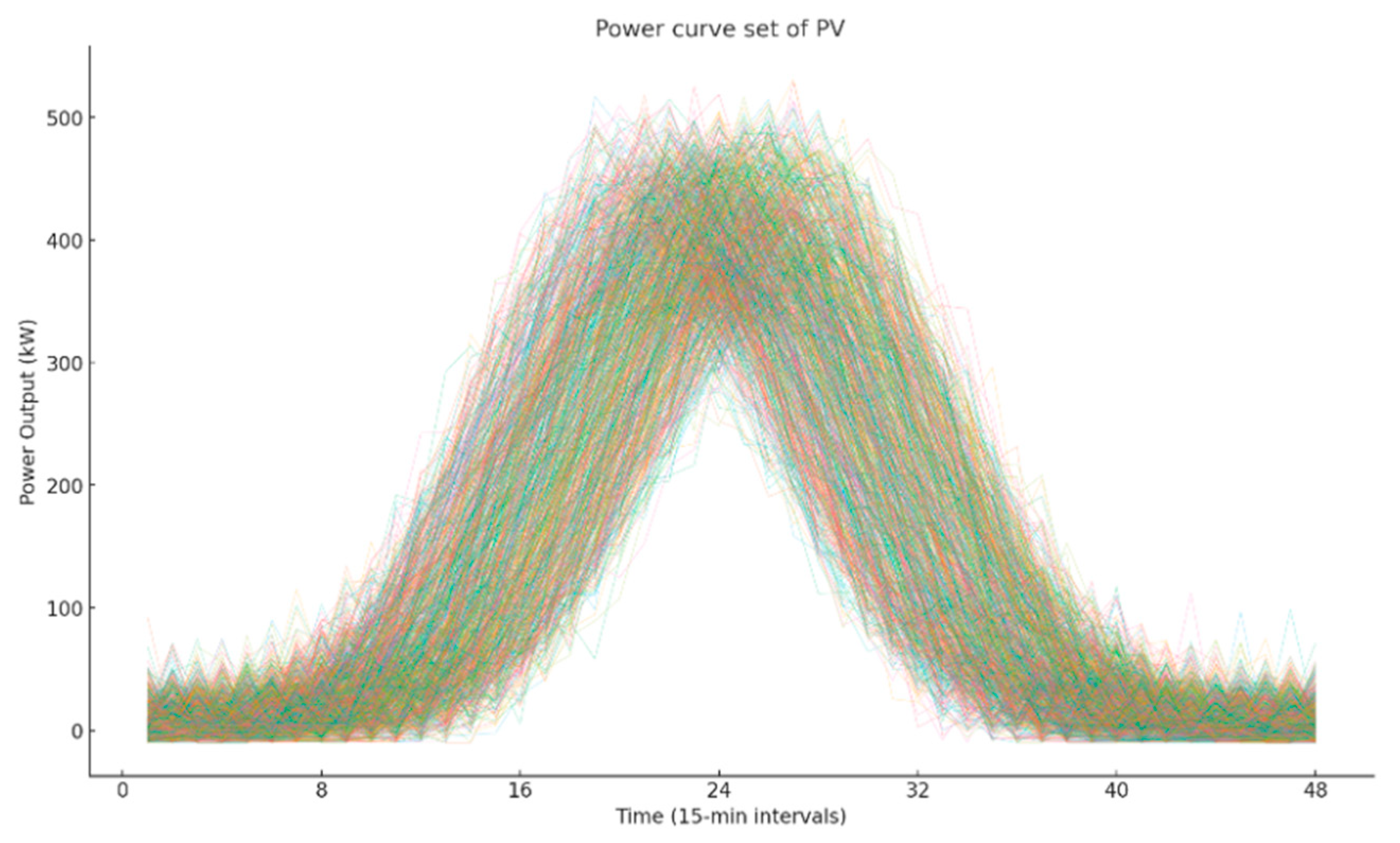
Figure 1. 1000 photovoltaic power generation curves.
Energies 18 05218 g001
Figure 2. 100 photovoltaic power generation curves.
Energies 18 05218 g002
Figure 3. 10 photovoltaic power generation curves.
Energies 18 05218 g003
Figure 4. 1000 wind power generation curves.
Energies 18 05218 g004
Figure 5. 100 wind power generation curves.
Energies 18 05218 g005
Figure 6. 10 wind power generation curves.
Energies 18 05218 g006
Figure 7. 1000 load demand curves.
Energies 18 05218 g007
Figure 8. 100 load demand curves.
Energies 18 05218 g008
Figure 9. 10 load demand curves.
Energies 18 05218 g009
Table 1. Installed Capacity of Renewable Energy and Load.
NoTypeCapacity (kW)
APV500
BPV500
CWind600
DWind600
EWind500
FLoad1500
Table 2. Key Parameters of the Transformer Model.
ParameterDescriptionValue
d_modelHidden layer dimension128
nheadNumber of attention head4
num_encoder_layersNumber of Encoder layers3
num_decoder_layersNumber of Decoder layers3
fn_dimFeed-forward network dimension2 × d_model
dropoutDropout rate0.1
max_seq_lenSequence length (time steps)96
output_dimOutput dimensionK × 3
Table 3. Results generated from 1000 input scenarios.
NoSchemeJcost (k$)JrampJrel (%)
1(0.22,0.51,0.27)1121.8210.22
2(0.28,0.57,0.15)992.55−5.31
3(0.23,0.54,0.23)1091.657.63
4(0.24,0.54,0.22)1061.725.37
5(0.22,0.51,0.20)1071.973.42
6(0.23,0.58,0.19)1031.741.93
Table 4. Results generated from 100 input scenarios.
NoSchemeJcost (k$)JrampJrel (%)
1(0.20,0.49,0.31)1212.809.32
2(0.19,0.53,0.28)1152.455.71
3(0.21,0.57,0.22)1092.155.64
4(0.24,0.54,0.22)1061.93−2.25
5(0.22,0.48,0.30)1171.874.52
6(0.25,0.54,0.21)1042.09−5.67
Table 5. Results generated from 10 input scenarios.
NoSchemeJcost (k$)JrampJrel (%)
1(0.22,0.52,0.16)952.83−2.91
2(0.18,0.49,0.33)1253.3511.52
3(0.23,0.53,0.24)1062.285.71
4(0.21,0.61,0.18)1023.222.38
5(0.28,0.51,0.21)1041.857.65
6(0.26,0.58,0.16)971.97−4.77
Disclaimer/Publisher’s Note: The statements, opinions and data contained in all publications are solely those of the individual author(s) and contributor(s) and not of MDPI and/or the editor(s). MDPI and/or the editor(s) disclaim responsibility for any injury to people or property resulting from any ideas, methods, instructions or products referred to in the content.