Article

A Hybrid Framework for Offshore Wind Power Forecasting: Integrating CNN-BiGRU-XGBoost with Advanced Feature Engineering and Analysis

1
Shanghai Engineering Research Center of Marine Renewable Energy, Shanghai 201306, China
2
College of Engineering Science and Technology, Shanghai Ocean University, Shanghai 201306, China
*
Author to whom correspondence should be addressed.
Energies 2025, 18(19), 5153; https://doi.org/10.3390/en18195153 (registering DOI)
Submission received: 19 August 2025 / Revised: 11 September 2025 / Accepted: 17 September 2025 / Published: 28 September 2025

Abstract

This paper proposes a hybrid forecasting model for offshore wind power, combining CNN, BiGRU, and XGBoost to address the challenges of fluctuating wind speeds and complex meteorological conditions. The model extracts local and temporal features, models nonlinear relationships, and uses residual-driven Ridge regression for improved error correction. Real-world data from a Jiangsu offshore wind farm in 2023 was used for training and testing. Results show the proposed approach consistently outperforms traditional models, achieving lower RMSE and MAE, and R2 values above 0.98 across all seasons. While the model shows strong robustness and accuracy, future work will focus on optimizing hyperparameters and expanding input features for even broader applicability. Overall, this hybrid model provides a practical solution for reliable offshore wind power forecasting.

1. Introduction

Offshore wind power has become a major focus for wind energy development, particularly in coastal nations and regions. Today, the global cumulative installed capacity has reached 64.31 GW. Offshore sites offer several key advantages over onshore wind farms, including more abundant wind resources, higher energy yields, more stable operation, and longer turbine lifespans. As a result, there is a clear global trend moving from land-based to offshore wind farm construction. However, forecasting offshore wind power remains a significant challenge due to the intermittent and uncontrollable nature of wind, as well as the complexity of weather conditions. The existing forecasting methods can be broadly categorized into two types: physical models and statistical models [1]. Physical models, which rely on numerical weather prediction (NWP) techniques, have been widely used for medium- and long-term forecasting. Commonly used tools include the Weather Research and Forecasting (WRF) model, Computational Fluid Dynamics (CFD), and the Global Forecast System (GFS) [2]. These models can improve forecasting accuracy, particularly in complex climates and landscapes. However, they depend heavily on accurate and detailed meteorological data, which may not always be available. Additionally, they require significant computational resources, and the forecasts can be sensitive to errors in input data. In contrast, statistical models such as the Autoregressive Integrated Moving Average (ARIMA) model [3], multiple linear regression [4], and Support Vector Machines (SVM) [5] use historical wind speed and power generation data to predict future outputs. While computationally less demanding, these models often struggle in extreme weather conditions, where their accuracy can degrade.
A variety of machine learning and deep learning techniques have emerged to address the limitations of traditional models. For example, a model combining learnable wavelet decomposition and sparse self-attention mechanisms was proposed to improve ultra-short-term wind power forecasting [6]. While this model offers better feature extraction capabilities, it remains complex and less robust when faced with sudden, non-periodic weather changes. Similarly, a multi-scale convolutional neural network (CNN) combined with residual structures [7] boosts short-term prediction accuracy but fails to fully capture the long-term temporal dependencies inherent in wind power data. Further advancements have been made with models like XGBoost, which optimize model parameters using techniques like Differential Evolution [8]. While this improves forecasting accuracy, it struggles with sequential dependencies and natural temporal fluctuations in wind power data. Hybrid models that combine methods such as CNNs, Gated Recurrent Units (GRUs), and attention mechanisms [9], or data fusion approaches with XGBoost [10], have been shown to improve performance. However, these models often focus on either spatial or temporal features separately, rarely integrating both, and their complexity can limit their practical applicability. Moreover, many models lack systematic parameter selection, multi-level feature fusion [11], or automated hyperparameter tuning, leading to limited generalizability across different datasets and environments.
While these advances in machine learning have made significant contributions to wind power forecasting, several challenges remain. First, most current models focus on extracting either spatial or temporal features, rather than effectively combining both to model the complex dynamics of wind power data. Additionally, existing models tend to be computationally expensive and are often tailored to specific regions or conditions, limiting their generalizability. Moreover, few studies have explored the use of outlier detection and residual error correction mechanisms in combination with these advanced models, which could potentially improve forecasting performance over long-term periods.
Recently, Large Language Models (LLMs) have gained significant attention in natural language processing (NLP) and AI-driven domains [12]. These models have also begun to make their way into power system forecasting, aiding tasks such as electricity price prediction and market behavior analysis. Notably, recent studies have explored the integration of multiple techniques, such as Bidding Behavior Agents and Market Sentiment Agents, which leverage LLMs to predict electricity prices and understand market dynamics. These approaches have been shown to effectively handle complex, nonlinear relationships in time-series data for power forecasting [13]. However, the application of LLMs in wind power forecasting, particularly in offshore settings, remains underexplored.
To address these challenges and research gaps, this study introduces a hybrid forecasting model that combines Convolutional Neural Networks (CNN), Bidirectional Gated Recurrent Units (BiGRU), and XGBoost. This model is designed to extract both spatial and temporal features, model nonlinear relationships, and capture dynamic changes in wind power data. In addition, we introduce a residual correction mechanism that helps reduce the accumulation of prediction errors over time. The proposed model avoids unnecessary complexity, striking a balance between accuracy and computational efficiency. This work aims to bridge the gap between existing forecasting techniques by integrating multiple model components and outlier detection mechanisms, providing a more robust solution for offshore wind power forecasting.

2. Wind Power Data Analysis and Preprocessing Methods

2.1. Data Source

This study uses data from an offshore wind farm in Jiangsu Province, China. The dataset covers the entire year of 2023. The wind turbines at this site have a total rated capacity of 48 MW. Measurements were taken every 15 min, resulting in 35,037 time-stamped records. The dataset includes wind power output and several meteorological variables, such as wind speed, temperature, and precipitation. For model development and evaluation, we randomly split the data into training and test sets with an 80:20 ratio.

2.2. Correlation Analysis

To examine the relationships between variables, we used the Pearson correlation coefficient. Environmental factors can affect wind power output in different ways. Measuring these connections helps us choose the right input features for the model [14]. The Pearson correlation coefficient ranges from −1 to 1 and shows both the strength and direction of a linear relationship. A value close to 1 means a strong positive link. A value near −1 means a strong negative link. The formula for the Pearson correlation coefficient is shown in Equation (1):
r x y = i = 1 n ( x i x ¯ ) ( y i y ¯ ) i = 1 n ( x i x ¯ ) 2 i = 1 n ( y i y ¯ ) 2
As shown in Figure 1, the correlation heatmap highlights a strong positive relationship between wind power output and wind speed measured at 100 m. The correlation coefficient for this pair is 0.7. Wind speed at 10 m also shows a similar strong association with wind power output. These results confirm that wind speed, at both heights, is a key factor in wind power generation. This finding matches the well-known view that wind speed is the main driver behind the changes and levels of wind power output.

2.3. Data Processing

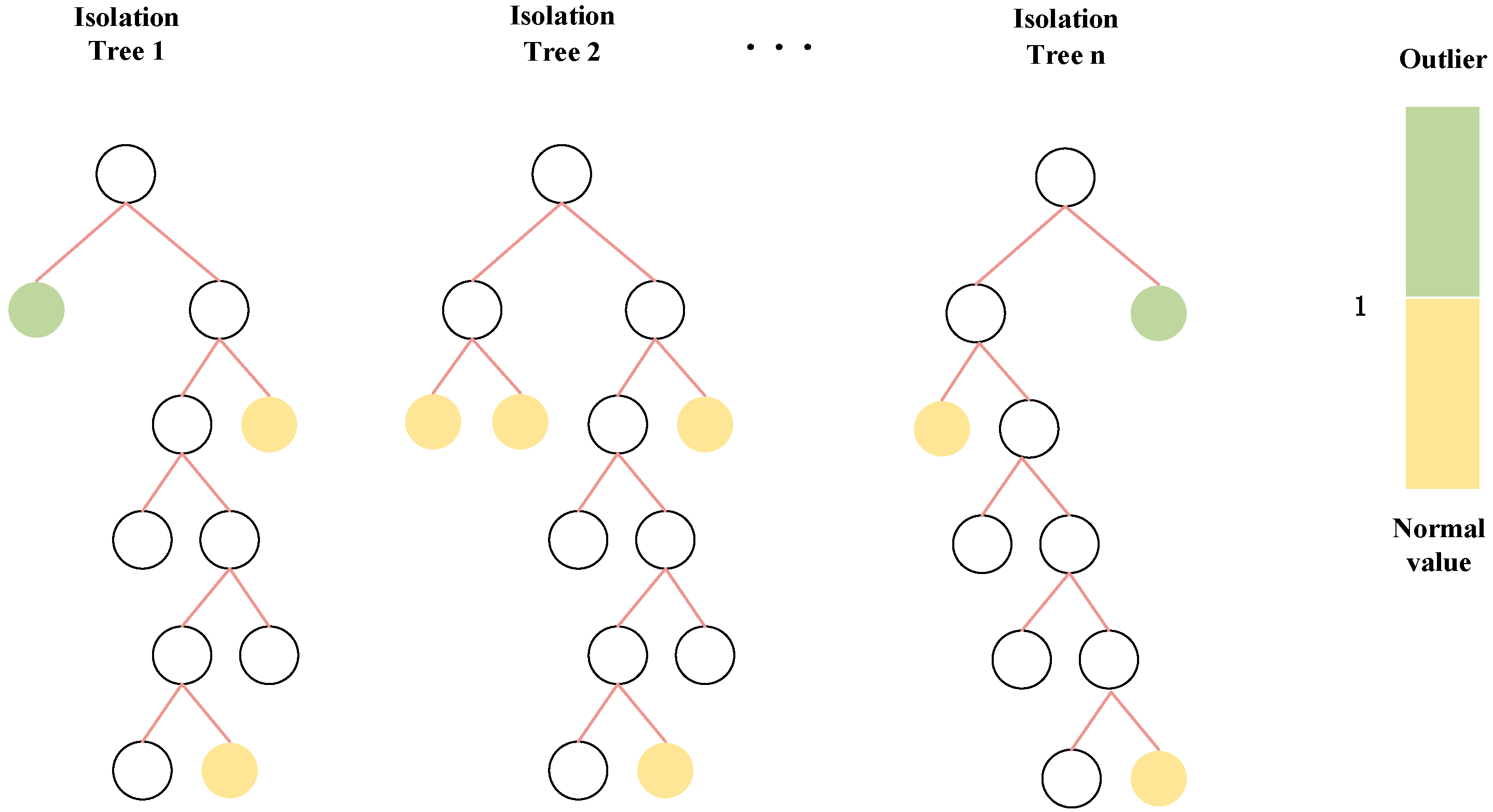
In offshore wind power forecasting, meteorological and power output data can contain outliers. These outliers may result from sensor malfunctions or sudden weather changes. Such data points can disrupt model training and reduce forecasting accuracy. To solve this problem, we used the Isolation Forest algorithm to detect and remove anomalies. Isolation Forest is an unsupervised method for anomaly detection. It works by recursively splitting the data into smaller parts. Outliers, which differ greatly from most samples, are easier to isolate and usually appear at the edges of the data distribution. In this study, we set a contamination rate of 5% to find and remove abnormal data points. Figure 2 illustrates how the Isolation Forest algorithm works. Each data point receives an anomaly score, which helps reliably identify and filter out outliers.
During the data preprocessing stage, all input features were standardized by subtracting the mean and dividing by the standard deviation of each dimension, resulting in zero mean and unit variance. This procedure not only mitigates the imbalance caused by heterogeneous feature scales during model training but also improves the training stability and convergence speed of CNN and BiGRU. Although XGBoost is relatively insensitive to feature scaling, maintaining a consistent feature distribution ensures better comparability when it is integrated with deep learning models.
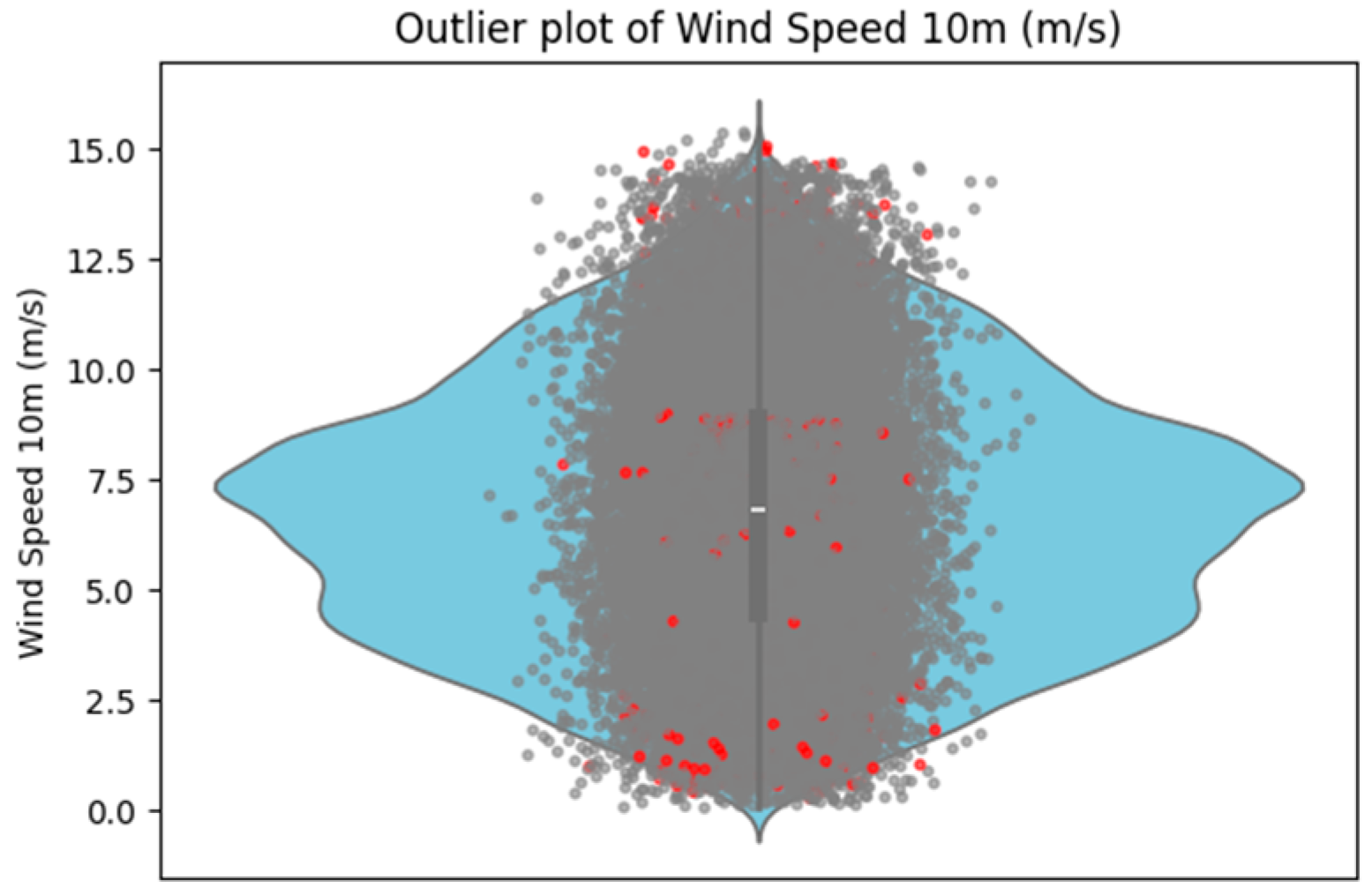
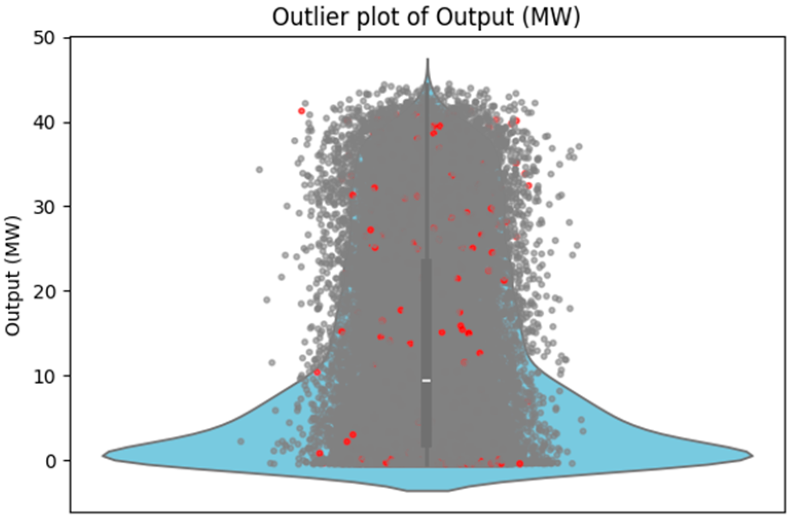
The Pearson correlation analysis shows that both 10 m and 100 m wind speeds have strong positive correlations with power output. These two wind speeds have the highest correlation coefficients among all variables. To illustrate the outlier detection process, we created violin plots for these three variables. In these plots, red markers represent outliers, while gray markers show normal data points. Figure 3, Figure 4 and Figure 5 display these visualizations and highlight the distribution and characteristics of the detected outliers. After identifying the outliers, we replaced all anomalous values with the median of the corresponding feature. This method reduces the effect of extreme values and keeps the overall data distribution intact.

2.4. Experimental Setup

In this study, we use a one-step short-term wind power prediction approach. The prediction time horizon is the wind power output for the next 15 min. In this paper, we use data from the past 24 h, such as hourly wind speed, temperature, and other data as input features. The training and testing sets are generated through a sliding window strategy, where the time window is moved forward by one time step each time, generating the input features and prediction targets for the next time step.
Additionally, the wind power output is standardized during the training process, with normalization applied to the target using the mean and standard deviation of the training set. After the model prediction, the results are inverse normalized to restore them to the actual wind power output values. These settings ensure the reproducibility of the experiment and align with real-world application scenarios.

3. Research Methods

3.1. CNN-BiGRU

Convolutional Neural Networks (CNNs) were first introduced by Yann LeCun in 1998 [15]. Since then, they have been used in many fields, including time series analysis. In meteorological data, local patterns can hold key information, as important changes often happen over short periods. CNNs use convolutional operations to extract these local features. This allows the model to capture short-term fluctuations in wind speed effectively. As convolutional kernels move across the input sequences, they can recognize similar patterns at different time steps. This reduces the number of parameters and improves the model’s ability to generalize.
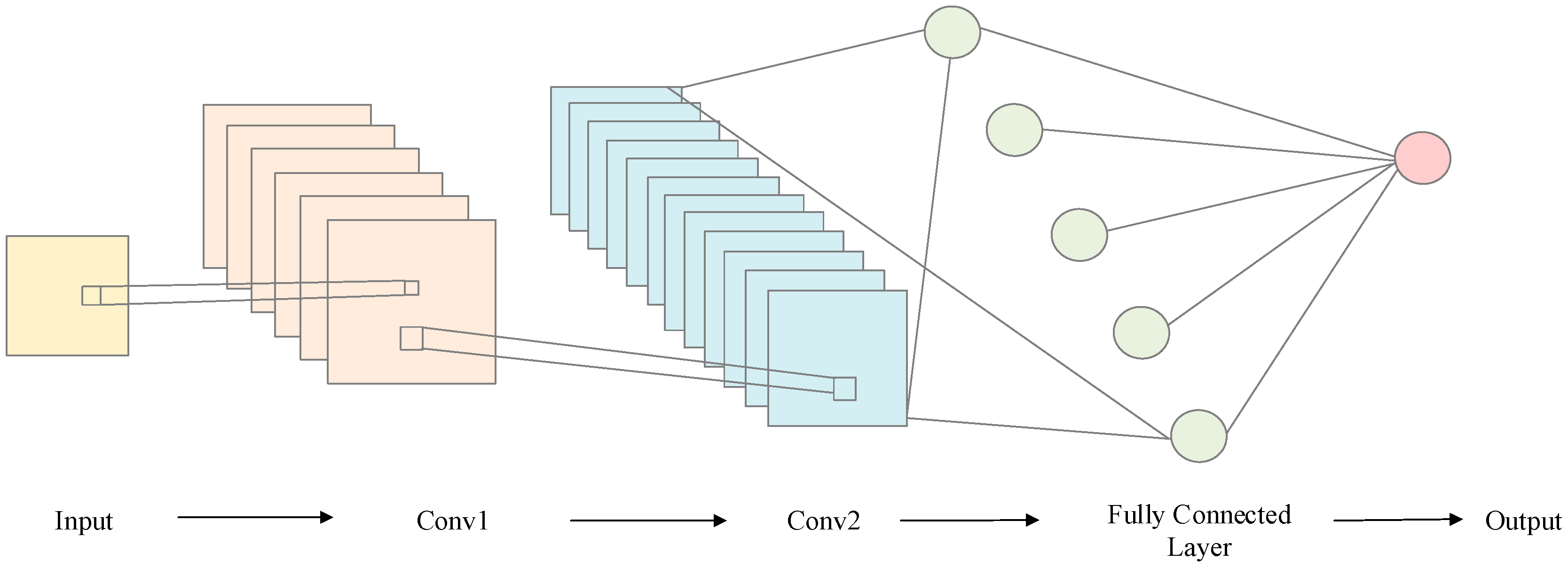
In this study, we use two convolutional layers to extract basic edge information and local temporal patterns from the data. Traditional CNNs often use pooling layers after convolution to down sample data. Pooling reduces the number of parameters and computational cost, and it can also help with generalization. However, for wind power forecasting, pooling layers can remove fine-grained temporal details. These details are important for modeling the rapid and extreme changes in wind power output. For this reason, our model does not use pooling layers, helping preserve important local temporal features. Figure 6 shows this design.
Both the first and second convolutional layers in our model use the Leaky ReLU activation function after convolution. Unlike standard ReLU, Leaky ReLU allows a small, non-zero gradient when the input is negative. This helps prevent the issue of vanishing gradients. Leaky ReLU is especially useful for processing features with possible negative values, such as wind speed. It also helps the model capture more complex nonlinear patterns in the data. The formula for the Leaky ReLU activation function appears in Equation (2):
f ( x ) = x , x > 0 a x , x 0
where x is the input and a is the slope of the gradient in the negative input region.
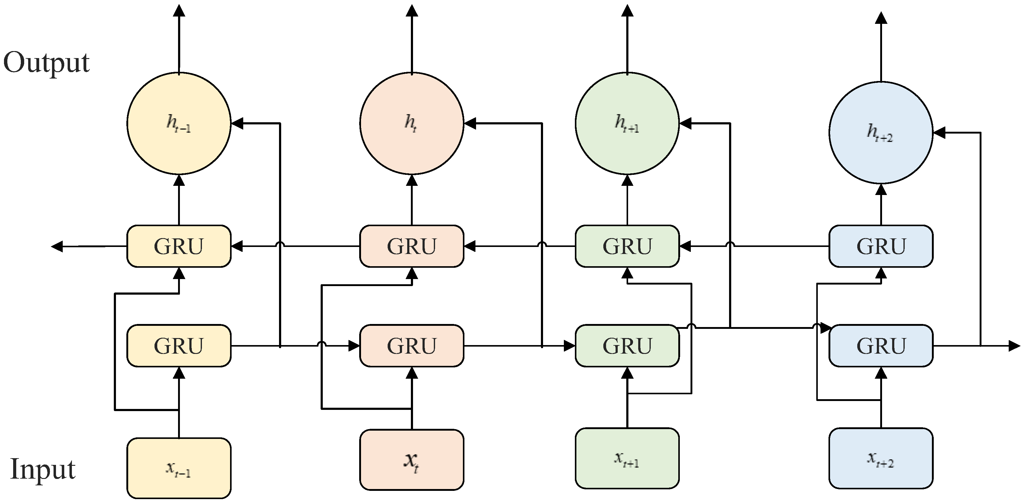
After the convolutional layers, the model includes a bidirectional gated recurrent unit (BiGRU) to process the time series data further [16]. The CNN modules first extract local features from the raw meteorological inputs. Then, the BiGRU models the temporal relationships within these features. A bidirectional GRU goes beyond the standard unidirectional GRU by using two GRU networks in parallel. One processes the sequence from past to present, while the other works from future to present. At each time step, the model combines the outputs from both directions and sends them to the next layer. This setup helps the model gather information from both past and future data points. By integrating context from both directions, the BiGRU provides a better understanding of global temporal patterns in the data. As a result, it improves prediction accuracy. Figure 7 shows how the bidirectional GRU works.
During model training, multiple strategies were employed to mitigate the risk of overfitting. An early stopping mechanism was introduced, using the validation loss as the monitoring criterion; training was terminated when no improvement was observed for several consecutive epochs, and the model weights were rolled back to the best-performing state. In addition, an adaptive learning rate decay strategy was adopted, whereby the learning rate was automatically reduced when the validation error plateaued, thus enhancing convergence stability. L2 regularization was applied to the convolutional, BiGRU, and fully connected layers, while both dropout and recurrent dropout were incorporated into the bidirectional GRU layers to further alleviate overfitting. Finally, random search combined with validation-based selection was used to constrain model capacity—such as the number of convolutional filters, GRU, tree depth, and subsampling rate—ensuring that the model complexity was commensurate with the data scale.

3.2. XGBoost Algorithm

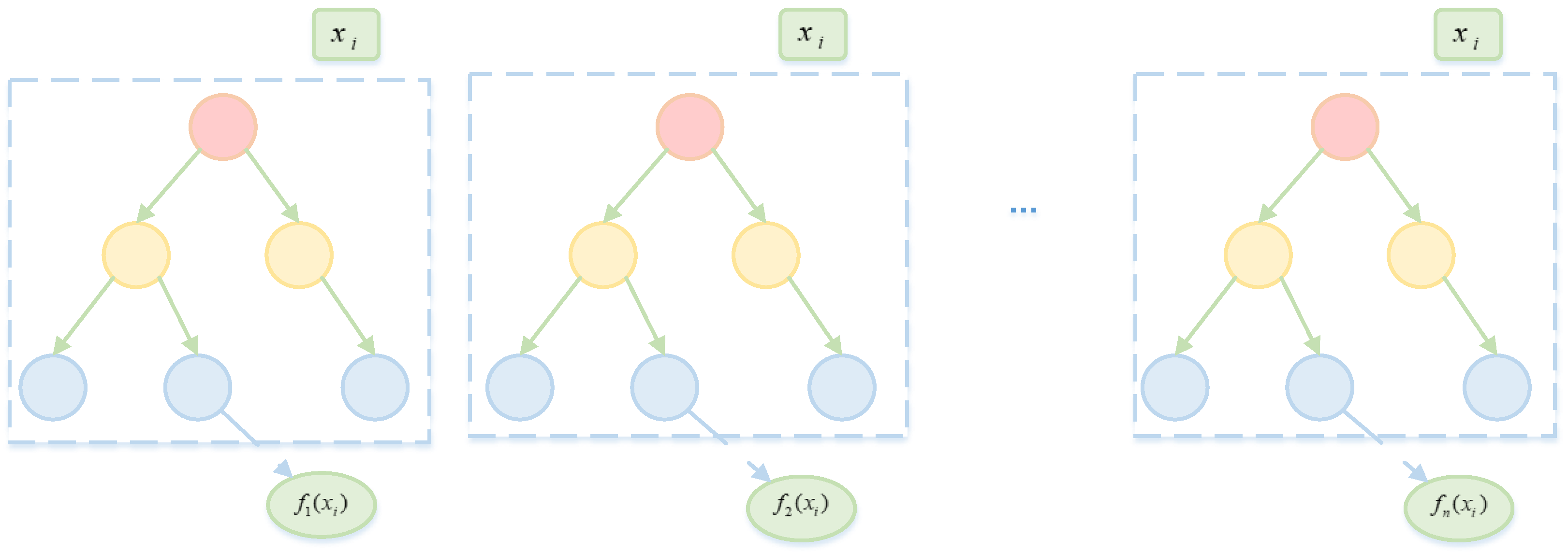
XGBoost is an improved form of the Gradient Boosting Decision Tree (GBDT) algorithm. The prediction output is shown in Equation (3). XGBoost boosts predictive accuracy by reducing residuals through several decision trees, one after another. Each new tree learns to fit the errors made by the previous tree. The model repeats this process, steadily minimizing the residuals and improving prediction accuracy. Figure 8 illustrates how the XGBoost algorithm works.
y ^ i = i = 1 N f n ( x i )
where y ^ i is the prediction of the first j sample, f n ( x i ) is the prediction of the first n tree for the sample i , and N is the total number of trees.
In the XGBoost framework, each decision tree comes from a function space, and the model uses gradient boosting for optimization. This method allows each new tree to minimize the loss function at each step. For regression tasks, XGBoost uses both first-order and second-order gradient information. It calculates the gradient and the second-order derivative (Hessian) of the loss function, as shown in Equations (4) and (5). By using this extra derivative information, XGBoost updates its parameters more efficiently and builds new trees faster. This helps the model reach the best solution more quickly.
g i = L ( y i , y ^ i ) y ^ i
h i = 2 L ( y i , y ^ i ) y ^ i 2
where g i is the gradient of the loss function, h i is the second-order derivation of the loss function, y i is the true value of the ith sample, and y ^ i is the predicted value of the model.

3.3. Randomized SearchCV

In this study, we used Randomized SearchCV for hyperparameter optimization. This method samples and tests multiple parameter combinations from a defined search space to find the best settings for the model. After defining the parameter space, Randomized SearchCV randomly picks several sets of hyperparameters and performs cross-validation on each. During cross-validation, the data is split into three folds. In each round, two folds are used for training and the third for validation. This approach reduces the chance of overfitting to any single data split and improves the robustness and generalizability of the chosen hyperparameters. Figure 9 shows the overall optimization process.

3.4. Ridge Regression

In this study, Ridge regression is selected as the meta-learner. The input of the stacked layer not only includes the prediction results of each base learner but also their residuals. There is often strong multicollinearity among these features. Ridge regression effectively alleviates the overfitting problem caused by overly strong feature correlation by introducing L2 regularization into the loss function and can achieve a relatively balanced weight distribution among multiple related features. In contrast, Lasso regression [17], due to the use of L1 regularization, tends to compress the coefficients of some related features to zero. Although this is beneficial for feature selection, it is prone to losing valuable information in scenarios where features are highly correlated, leading to model instability. ElasticNet [18] combines L1 and L2 regularization, but it may still be affected by L1 sparsity in weight distribution and its performance is not as stable as that of Ridge.
Ridge regression l takes in the prediction outputs and their residuals from earlier stages, creating a four-dimensional feature vector for fusion. By including residual information, the model can correct errors missed in previous predictions and better learn hidden error patterns. This residual-driven correction adds another layer of learning, helping the model handle predictive blind spots more effectively [19]. Ridge regression also controls model complexity by adding an L2 regularization term to the loss function. This term penalizes large regression coefficients, as shown in Equation (6).
L θ = i = 1 n ( y i y ^ i ) 2 + α j = 1 p θ j 2
where y i is the true value of the i-th sample, y ^ i is the predicted value of the model, θ j is the regression coefficient of the model, α is the regularized hyperparameter, n is the total number of samples, and p is the total number of features.
During the fusion stage, we not only combined the predictions of the basic models (CNN-BiGRU and XGBoost), but also took their residuals as additional features, as shown in Equation (7).
r i ( m ) = y i y ^ i ( m )
where y i denotes the true target value of the i-th sample, and y ^ i ( m ) represents the prediction of the base model.
These residual terms capture the systematic errors of each base learner, providing complementary information that is not available from the raw predictions alone. For each sample, we therefore construct a four-dimensional fusion feature vector, as shown in Equation (8). This vector simultaneously encodes the predictive outputs and their associated error patterns. Ridge regression is then employed as the meta-learner to model the linear relationship between these enriched features and the ground truth. By incorporating residual information, the meta-learner can better correct for systematic biases in the base models, thereby improving both predictive accuracy and robustness of the final ensemble.
z i = [ y ^ i C N N B i G R U , y ^ i X G B o o s t , r i C N N B i G R U , r i X G B o o s t ]

4. Construction and Evaluation of the Forecasting Model

4.1. Model Construction

The proposed model includes many tunable parameters. These include the number of convolutional filters, the number of hidden units, the learning rate, and the maximum tree depth. Each parameter can have a significant impact on forecasting performance [20]. Table 1 lists the specific model and system settings used in this study. All experiments ran on a laptop with a 64-bit Windows operating system, an NVIDIA GeForce GTX 1050 Ti GPU, an Intel Core i7-8750H @ 2.20 GHz processor, and 8 GB of RAM. The software environment was Python 3.11. Because parameter selection is stochastic, we carried out systematic hyperparameter optimization to ensure the best forecasting results.
The construction steps of the CNN-BiGRU-XGBoost model are as follows:
(1)
Select the number of filters and kernel sizes for the Convolutional Neural Network (CNN). Unlike conventional CNN structures, the pooling layer is removed in this design. For the Bidirectional GRU (BiGRU), the number of units in the two layers and the dropout rate are determined to construct a deep learning model capable of extracting local features and modeling both short- and long-term dependencies in time series data. The workflow of the CNN-BiGRU forecasting model is shown in Figure 10.
(2)
Introduce XGBoost as the base learner. Key parameters such as learning rate, maximum tree depth, minimum child weight, subsample ratio, feature sampling ratio, and maximum number of iterations are selected. XGBoost’s powerful nonlinear modeling capability is leveraged to further improve model performance, forming a second independent prediction pathway.
(3)
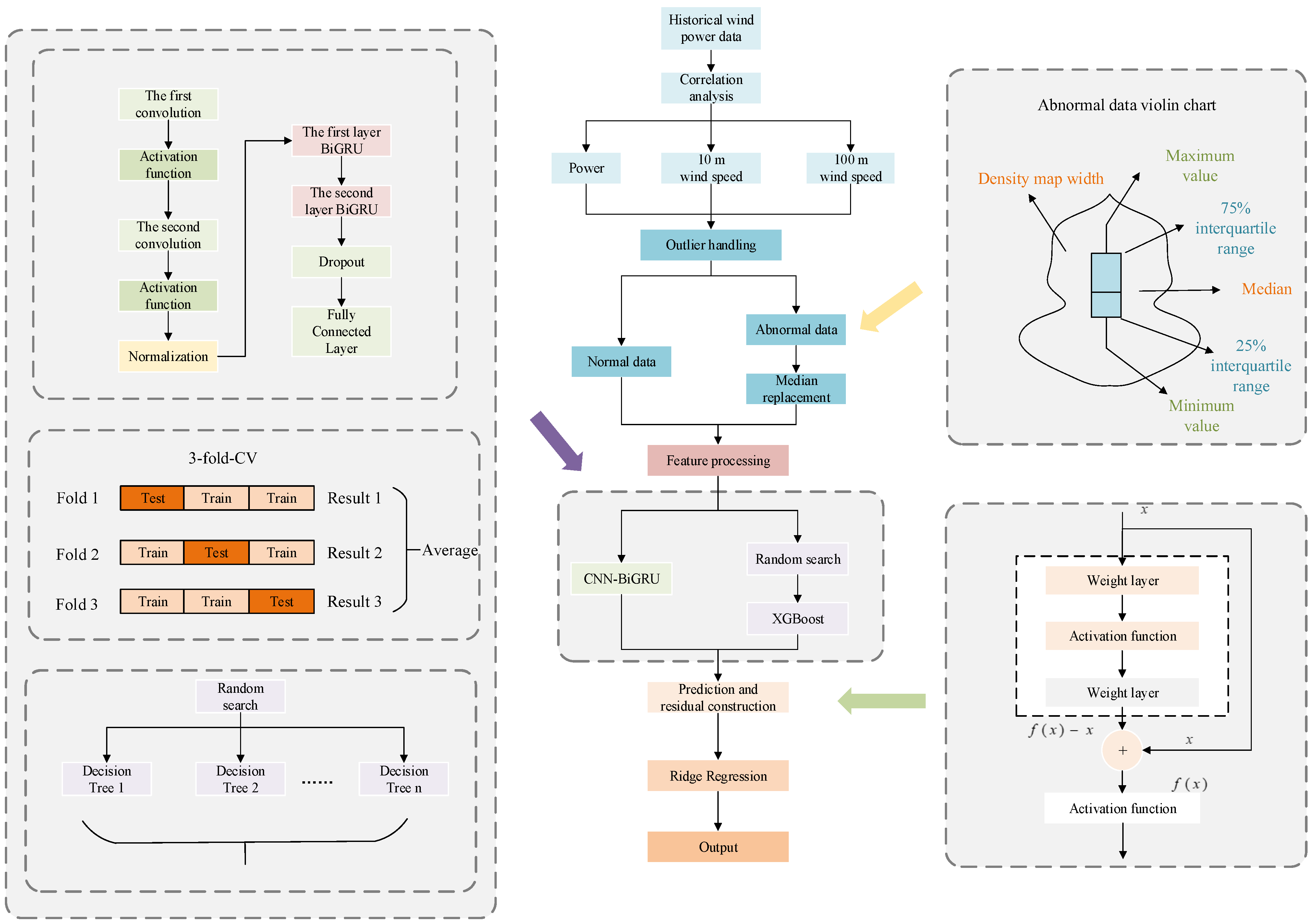
The prediction results from the CNN-BiGRU and XGBoost models, along with their corresponding residuals, are used as input features to form a four-dimensional fusion vector. Ridge regression is then employed to enhance convergence efficiency and improve the model’s ability to fit error structures. The overall modeling process is illustrated in Figure 11.

4.2. Evaluation Metrics

In the task of wind power prediction, the selection of an appropriate evaluation index can effectively measure the accuracy and robustness of the model, so this time, four functions are selected to predict the wind power evaluation index, with the specific formula as follows:
(1)
Root Mean Square Error (RMSE)
The root mean square error is the square root of the mean square error, and can be shown in Equation (9):
R M S E = M S E = 1 n i = 1 n ( y i y ^ i ) 2
(2)
Mean Absolute Error (MAE)
The mean absolute error is the average of the absolute values of the differences between the predicted and actual values [21] and can be shown in Equation (10):
M A E = 1 n i = 1 n | y i y ^ i |
(3)
Coefficient of determination (R2)
The coefficient of determination is used as a measure of the explanatory power of the model, and its value ranges from 0 to 1 and can be shown in Equation (11):
R 2 = 1 i = 1 n ( y i y ^ i ) 2 i = 1 n ( y i y ¯ ) 2

4.3. Results Analysis and Discussion

To verify the settings of the contamination parameter for the outlier handling method using Isolation Forest, this study uses fixed contamination rates of 1%, 5%, and 10% to compare with the experiments without outlier handling. The evaluation criteria used are RMSE, MAE, and R2, as shown in Table 2. Based on the experimental results, it can be concluded that the 5% fixed contamination rate yields the best results. Additionally, this process is applied consistently and only on the training set, ensuring no leakage of test information.
To validate the rationale for adopting Ridge regression as the meta-learner, this study further compared its performance with other commonly used approaches, including Lasso regression and ElasticNet regression. As shown in Table 3, Ridge consistently achieved the best results in terms of RMSE and MAE, while maintaining a relatively high and stable R2. In contrast, both Lasso and ElasticNet tend to enforce sparsity on features, which leads to degraded performance when strong multicollinearity exists among predictors. Ridge, by effectively balancing predictive accuracy and stability, was therefore selected as the final meta-learner.
To test the effectiveness of the proposed baseline model for offshore wind power forecasting, we built several comparison models. These included LSTM, TNN, BiGRU, XGBoost, CNN-BiGRU, BiGRU-XGBoost, ARIMA-BiGRU-XGBoost, and SVM-BiGRU-XGBoost. We systematically compared the predictive performance of each model against the proposed hybrid model. Experiments were carried out for each season—spring, summer, autumn, and winter. For every season, the data was split into training and test sets for model development and evaluation.
Analysis of the results for all four seasons shows that the CNN-BiGRU-XGBoost model is highly effective at capturing wind power output fluctuations. The model’s predictions closely match the actual power measurements, especially during times of large changes, and show reduced prediction errors at extreme values. Across different seasons, the proposed model maintains steady performance. It performs well in both stable conditions (spring and autumn) and in the more variable conditions of summer and winter. The SVM component does provide some nonlinear mapping ability, allowing it to handle moderately complex patterns. However, it is less flexible than the convolutional neural network in highly dynamic situations. As a result, the SVM-BiGRU-XGBoost model is less accurate during extreme events and rapid changes, suggesting it has limitations in such cases. Compared with other benchmark models, the CNN-BiGRU-XGBoost model has smaller error fluctuations and better overall prediction performance. Table 4 summarizes the quantitative error metrics for each model.
The results in Table 4 show that the CNN-BiGRU-XGBoost model consistently outperforms both ARIMA-BiGRU-XGBoost and SVM-BiGRU-XGBoost across all four seasons. It achieves stable and low error metrics. For example, the RMSE values for the CNN-BiGRU-XGBoost model are 1.5131, 1.4962, 1.5565, and 1.6479 for spring, summer, autumn, and winter, respectively. These values represent an average RMSE reduction of about 66% compared to ARIMA-BiGRU-XGBoost and around 53% compared to SVM-BiGRU-XGBoost. For MAE, the CNN-BiGRU-XGBoost model also shows an average reduction of more than 60%. In addition, the R2 values for the proposed model always remain above 0.98. In contrast, the lowest R2 value for the ARIMA-based model is only 0.7865, while the SVM-based model fluctuates between 0.89 and 0.94. These results highlight the superior predictive accuracy and greater seasonal robustness of the CNN-BiGRU-XGBoost model.
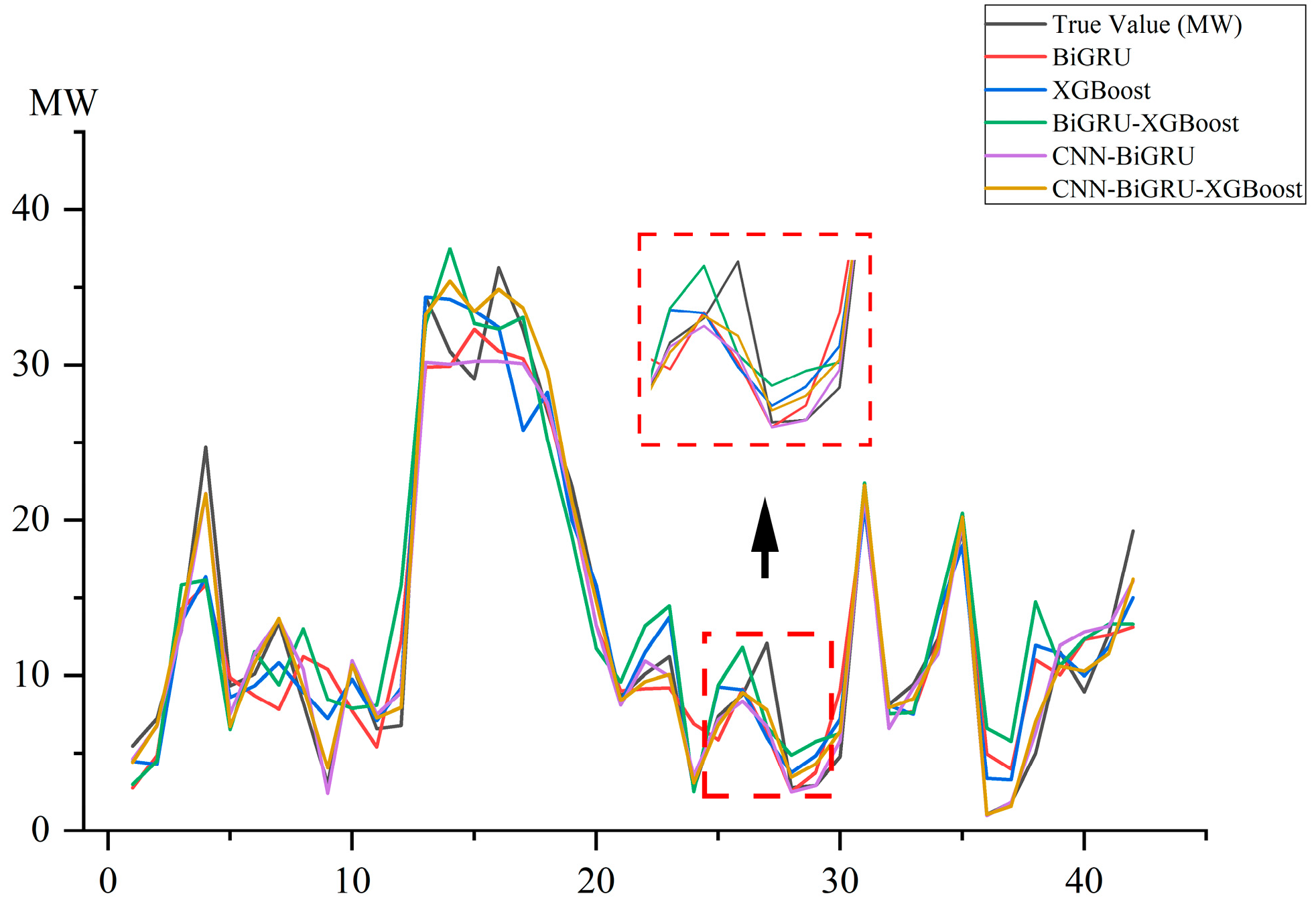
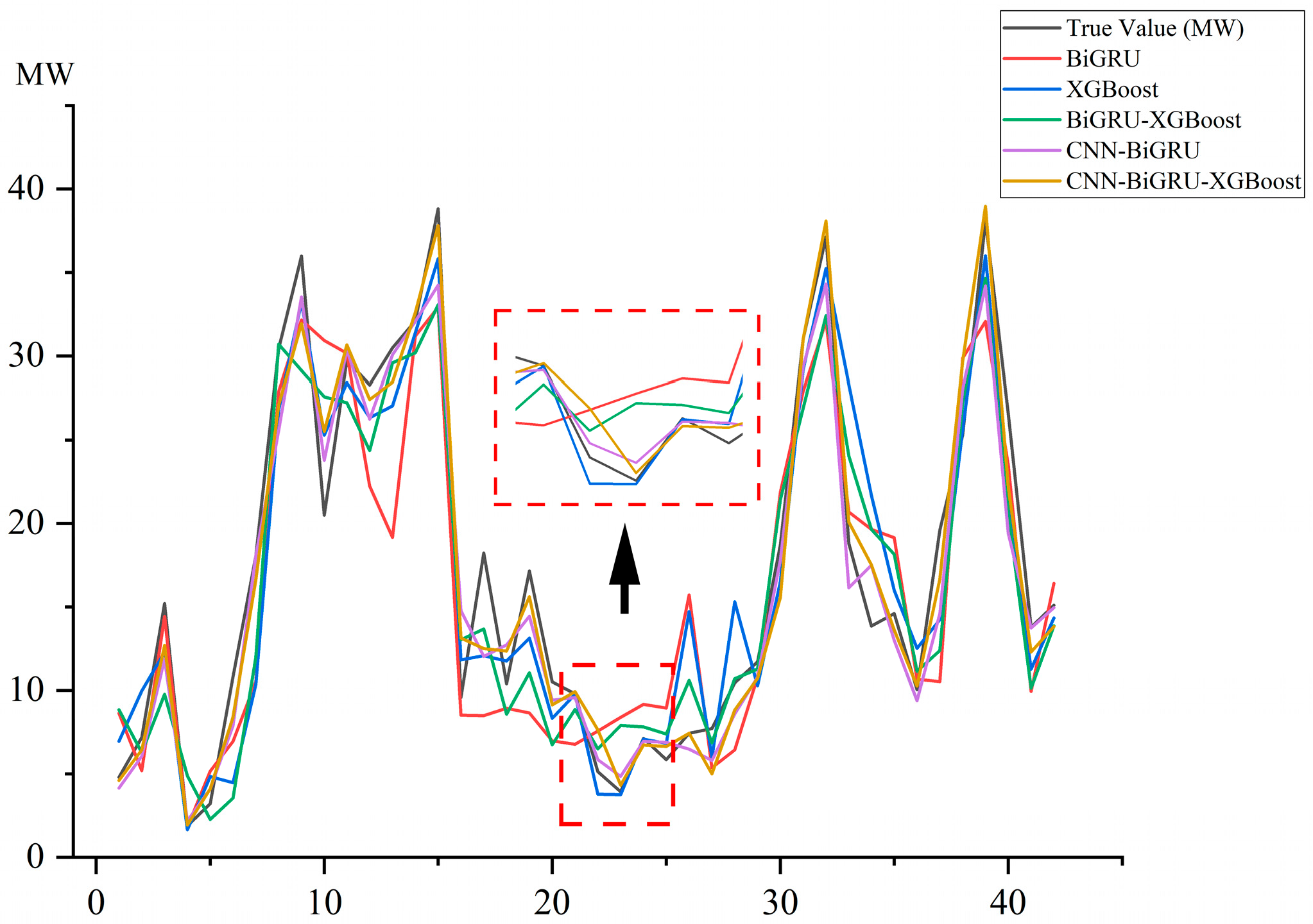
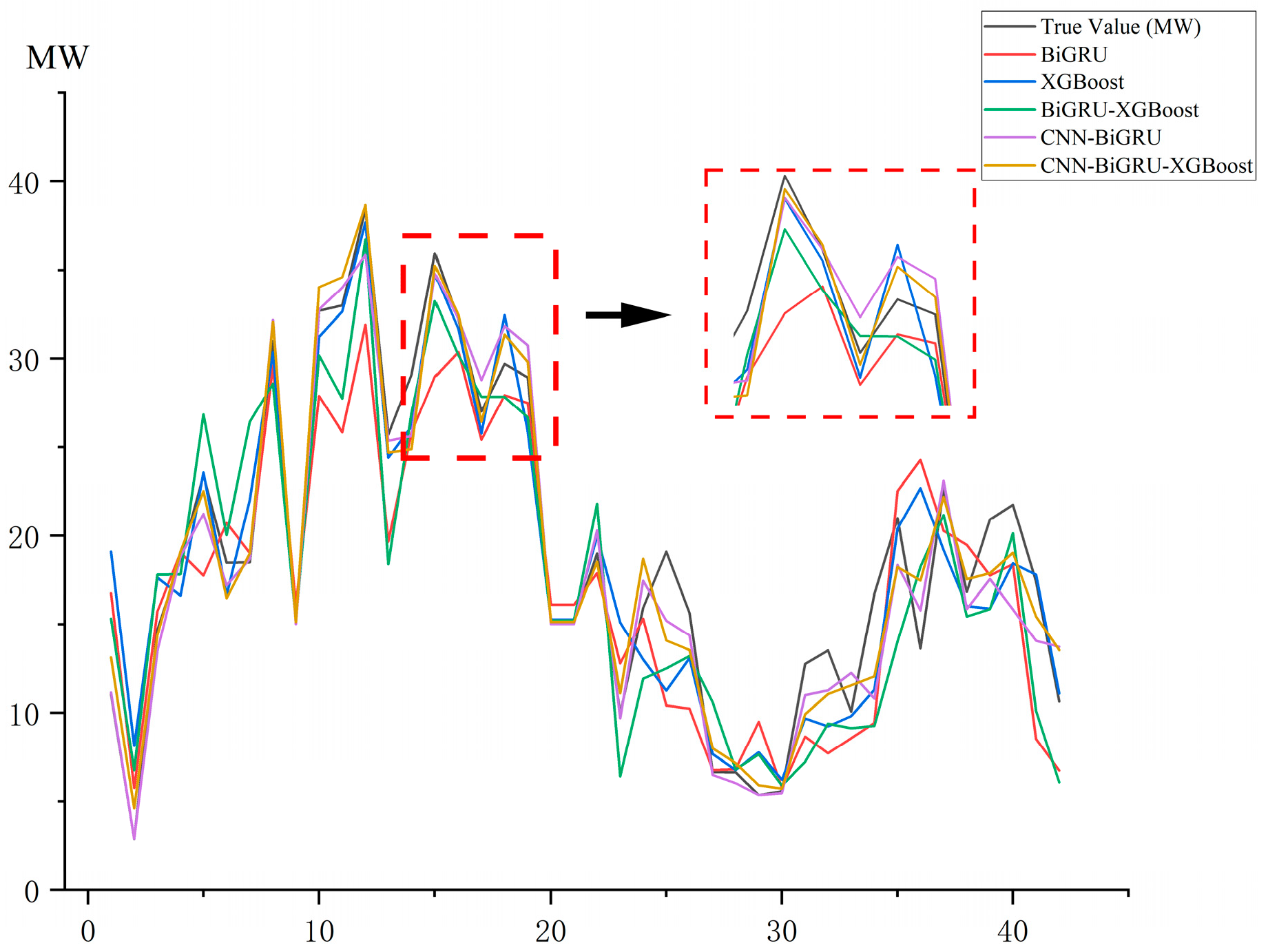
To comprehensively evaluate the performance of the models in wind power prediction, we compared five models, namely BiGRU, XGBoost, BigRU-XGBoost, CNN-BiGRU and CNN-BigRU-XGBoost, in spring, summer, autumn and winter, as shown in Figure 12, Figure 13, Figure 14 and Figure 15 and Table 5. In spring, when wind power output is relatively stable, all models generally follow the observed trend. However, CNN-BiGRU-XGBoost shows noticeably fewer local deviations, especially during minor fluctuations, which highlights the role of residual-driven Ridge regression in correcting systematic errors and maintaining smoother predictions. Summer is characterized by sharp ramping events caused by convective weather. In these conditions, BiGRU and XGBoost often lag behind sudden changes, producing large peak errors. By contrast, the proposed model tracks these ramping events more closely, owing to the CNN design without pooling layers that preserves short-term fluctuations and improves responsiveness to rapid variations. Autumn exhibits moderate variability, where capturing temporal dependencies is critical. CNN-BiGRU-XGBoost produces smoother transitions and fewer error spikes compared to CNN or BiGRU alone. This improvement reflects the contribution of the bidirectional GRU, which integrates contextual information from both past and future within the input window. Winter conditions present strong volatility and extreme dips in power output, which are challenging for all models. While baseline models show pronounced deviations in these extreme cases, CNN-BiGRU-XGBoost consistently maintains smaller errors and higher fidelity to the true curve. This robustness demonstrates the effectiveness of residual-enhanced fusion in mitigating bias accumulation under harsh meteorological conditions.
To further investigate the robustness of the proposed approach, segmented error metrics were calculated for peaks, valleys, and ramp events. As shown in Table 6. Error magnitudes increase under extreme operating conditions for all models, but CNN-BiGRU-XGBoost consistently outperforms the baselines. The largest gains appear in peak and ramp scenarios, where the absence of pooling layers in CNN helps capture short-term fluctuations and the residual-driven Ridge regression corrects systematic errors. Even in valley periods, where percentage-based errors are often inflated due to small denominators, the hybrid model achieves substantially smaller RMSE and MAE than ARIMA-BiGRU and SVM-BiGRU. These results highlight the model’s superior capability to handle non-stationary and volatile patterns in offshore wind power forecasting.
As shown in the tables, the CNN-BiGRU-XGBoost forecasting model consistently outperforms all other models in every performance metric. The predicted curves from this model closely match the actual observed values, accurately reflecting trend changes across all periods of fluctuation. By combining the temporal feature extraction power of deep learning with the structured feature processing strengths of XGBoost, the CNN-BiGRU-XGBoost model captures complex nonlinear temporal patterns and makes full use of the data’s structure. This leads to high predictive accuracy for both extreme values and minor fluctuations. These results highlight the model’s suitability for forecasting wind power in complex and dynamic environments.

5. Conclusions

In this study, we developed a hybrid forecasting model that combines CNN, BiGRU, and XGBoost to address the challenges of frequent wind speed fluctuations and complex meteorological conditions in offshore wind power forecasting. To improve error correction, we also included a residual-driven Ridge regression mechanism. The CNN layers extract key local features without losing important details, as pooling layers are omitted. BiGRU captures temporal dependencies, while XGBoost enhances modeling of nonlinear relationships. By fusing prediction results with residuals, the model reduces error accumulation and increases overall forecasting accuracy.
We tested the model using real-world data from an offshore wind farm in Jiangsu Province, covering all seasons in 2023. Results show that CNN-BiGRU-XGBoost consistently outperforms baseline models such as ARIMA and SVM in terms of RMSE, MAE, and R2. The model’s predictions closely follow the actual power output, showing excellent stability and generalization. However, there are still some limitations. This study used the data from the offshore wind farm in Jiangsu, China, in 2023 for verification, and the results were relatively good. However, due to the limited public availability of data on offshore wind farms at present, this model will be extended to different locations or other years for further testing in the future to evaluate its adaptability and robustness under different conditions. In this study, hyperparameter tuning relies on random search, and feature selection mainly focuses on basic variables such as wind speed and temperature. There are no more diverse data sources. In the future, more effective hyperparameter optimization methods, such as “Bayesian optimization” or “genetic algorithm”, can be explored to improve the tuning process. To support real-time deployment on edge devices, further model compression and acceleration are needed to promote low-latency and real-time prediction of smart grid devices.
In summary, the proposed CNN-BiGRU-XGBoost hybrid model demonstrates strong performance and wide applicability for wind power forecasting. It provides an effective solution for high-precision prediction in complex offshore settings and offers valuable insights for advancing renewable energy forecasting methods.

Author Contributions

Conceptualization, Y.L. and J.P.; data curation, J.P.; formal analysis, J.P. and J.W.; funding acquisition, Y.L.; investigation, J.P.; methodology, J.P.; project administration, Y.L. and J.P.; resources, J.P. and J.W.; software, J.P.; supervision, Y.L.; validation, J.P.; visualization, J.P. and J.W.; writing—original draft, J.P.; writing—review and editing, Y.L. and J.P. All authors have read and agreed to the published version of the manuscript.

Funding

This research was funded by the National Natural Science Foundation of China (No. 51876114) and the Shanghai Science and Technology Commission Funding Project, “Shanghai Marine Renewable Energy Engineering Technology Research Center” (19DZ2254800).

Data Availability Statement

The original contributions presented in the study are included in the article. Further inquiries can be directed to the corresponding author.

Conflicts of Interest

The authors declare that this study received funding from the National Natural Science Foundation of China (No. 51876114) and the Shanghai Science and Technology Commission Funding Project, “Shanghai Marine Renewable Energy Engineering Technology Research Center” (19DZ2254800). The funder was not involved in the study design, collection, analysis, interpretation of data, the writing of this article, or the decision to submit it for publication.

References

  1. Wu, K.; Yuan, Y.; Cheng, B.; Wu, J. Research of Wind Power Prediction Model Based on RBF Neural Network. In Proceedings of the 2013 International Conference on Computational and Information Sciences, Shiyang, China, 21–23 June 2013; pp. 237–240. [Google Scholar] [CrossRef]
  2. Artipoli, G.; Durante, F. Physical Modelling in Wind Energy Forecasting. Dewi Mag. 2014, 44, 10–15. [Google Scholar]
  3. Nayak, A.K.; Sharma, K.C.; Bhakar, R.; Mathur, J. ARIMA based statistical approach to predict wind power ramps. In Proceedings of the 2015 IEEE Power and Energy Society Conference, Denver, CO, USA, 26–30 July 2015; pp. 1–5. [Google Scholar]
  4. Shi, H.; Li, Z.; Ma, X. Wind power prediction based on DBN and multiple linear regression. Comput. Simul. 2023, 40, 90–95. [Google Scholar]
  5. Si, H. Research on Wind Power Prediction Algorithm Based on Support Vector Machine Theory. Master’s Thesis, North China University of Water Resources and Hydropower, Zhengzhou, China, 2019. [Google Scholar]
  6. Wang, M.; Rong, T.; Li, X.; Wei, C.; Zhang, A. Ultra-short-term prediction of offshore wind power based on learnable wavelet self-attention model. High Volt. Technol. 2024, 51, 1422–1433. [Google Scholar] [CrossRef]
  7. Yin, L.; Tong, B.; Li, W. Short-term wind power prediction based on multiscale convolutional-residual networks. Integr. Intell. Energy 2024, 47, 1–10. [Google Scholar] [CrossRef]
  8. Zhang, J.; Tian, H. Short-term wind power prediction based on DE-XGBoost. Inf. Technol. 2024, 7, 136–142. [Google Scholar]
  9. Ren, D.; Ma, J.; Liu, H.; Li, Y.; Chen, C.; Qin, T.; He, Z.; Wu, Q. The IVMD-CNN-GRU-Attention Model for Wind Power Prediction with Sample Entropy Fusion (December 2023). IEEE Access 2024, 12, 2169–3536. [Google Scholar] [CrossRef]
  10. Gao, J.; Ye, X.; Lei, X.; Huang, B.; Wang, X.; Wang, L. A Multichannel-Based CNN and GRU Method for Short-Term Wind Power Prediction. Electronics 2023, 12, 4479. [Google Scholar] [CrossRef]
  11. Jiang, J.; Wang, F.; Tang, R.; Zhang, L.; Xu, X. TS_XGB: Ultra-Short-Term Wind Power Forecasting Method Based on Fusion of Time-Spatial Data and XGBoost Algorithm. Procedia Comput. Sci. 2022, 199, 1103–1111. [Google Scholar]
  12. Yang, Z. Research on Short-Term Wind Power Prediction Based on Hybrid CNN-BiLSTM-AM Model. Master’s Thesis, Beijing Jiaotong University, Beijing, China, 2023. [Google Scholar]
  13. You, J.; Cai, H.; Shi, D.; Guo, L. An Improved Short-Term Electricity Load Forecasting Method: The VMD–KPCA–xLSTM–Informer Model. Energies 2025, 18, 2240. [Google Scholar] [CrossRef]
  14. Yang, M.; Chen, X.; Huang, B. Ultra-short-term multi-step wind power prediction based on fractal scaling factor transformation. J. Renew. Sustain. Energy 2018, 10, 053310. [Google Scholar]
  15. Lecun, Y.; Bottou, L.; Bengio, Y.; Haffner, P. Gradient-based learning applied to document recognition. Proc. IEEE 1998, 86, 2278–2324. [Google Scholar] [CrossRef]
  16. Zhou, G.B.; Wu, J.; Zhang, C.L.; Zhou, Z.H. Minimal gated unit for recurrent neural networks. Int. J. Autom. Comput. 2016, 13, 226–234. [Google Scholar] [CrossRef]
  17. Mauladdawilah, H.; Balfaqih, M.; Balfagih, Z.; Pegalajar, M.d.C.; Gago, E.J. Deep Feature Selection of Meteorological Variables for LSTM-Based PV Power Forecasting in High-Dimensional Time-Series Data. Algorithms 2025, 18, 496. [Google Scholar] [CrossRef]
  18. Shan, C.; Liu, S.; Peng, S.; Huang, Z.; Zuo, Y.; Zhang, W.; Xiao, J. A Wind Power Forecasting Method Based on Lightweight Representation Learning and Multivariate Feature Mixing. Energies 2025, 18, 2902. [Google Scholar] [CrossRef]
  19. Cozad, A.; Sahinidis, N.V.; Miller, D.C. Learning surrogate models for simulation-based optimisation. AIChE J. 2014, 60, 2211–2227. [Google Scholar] [CrossRef]
  20. Wei, F.; Zhang, Q.; Yin, Z. Development and application of national standards for big data system category. Inf. Technol. Stand. 2020, 7, 48–51. [Google Scholar]
  21. Lei, N.; Xiong, X. Suomi NPP VIIRS Solar Diffuser BRDF Degradation Factor at Short-Wave Infrared Band Wavelengths. IEEE Trans. Geosci. Remote Sens. 2016, 54, 6212–6216. [Google Scholar] [CrossRef]
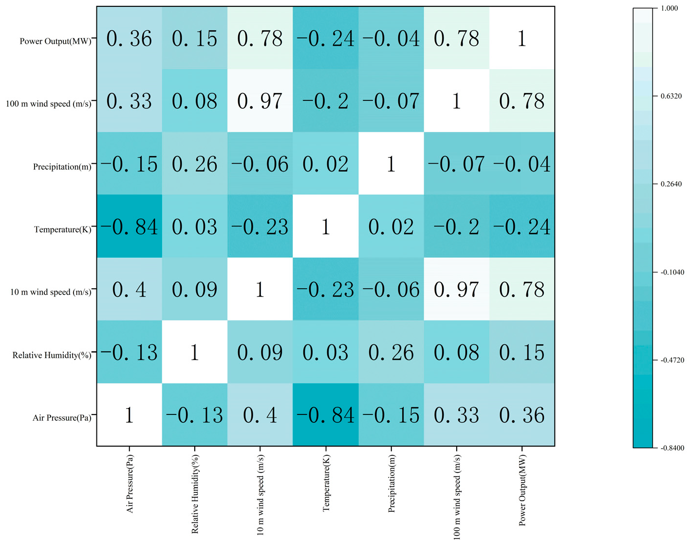
Figure 1. Pearson correlation coefficient heatmap.
Energies 18 05153 g001
Figure 2. Principal diagram of the Isolation Forest algorithm for outlier detection.
Energies 18 05153 g002
Figure 3. Outliers in 10 m wind speed.
Energies 18 05153 g003
Figure 4. Outliers in 100 m wind speed.
Energies 18 05153 g004
Figure 5. Outliers in power output.
Energies 18 05153 g005
Figure 6. Schematic diagram of the improved CNN architecture.
Energies 18 05153 g006
Figure 7. Schematic diagram of the bidirectional GRU (BiGRU) architecture.
Energies 18 05153 g007
Figure 8. Schematic diagram of the XGBoost algorithm.
Energies 18 05153 g008
Figure 9. Schematic diagram of the random search process.
Energies 18 05153 g009
Figure 10. Workflow diagram of the CNN-BiGRU forecasting model.
Energies 18 05153 g010
Figure 11. Workflow diagram of the wind power forecasting process.
Energies 18 05153 g011
Figure 12. Comparison of different models in spring (partial results).
Energies 18 05153 g012
Figure 13. Comparison of different models in summer (partial results).
Energies 18 05153 g013
Figure 14. Comparison of different models in autumn (partial results).
Energies 18 05153 g014
Figure 15. Comparison of different models in winter (partial results).
Energies 18 05153 g015
Table 1. Parameter settings for each component of the proposed model.
ModuleParameterSetting Value
ARIMAautoregressive order5
degree of differencing1
moving average order0
SVMpenalty coefficient100
insensitive to loss parameters0.01
CNNNumber of convolutional filters64, 128
Kernel size3
BiGRUNumber of units128, 64
Dropout rate0.3
XGBoostNumber of base learners300, 500 (tuning range)
Maximum tree depth6, 8 (tuning range)
Minimum child weight1, 5 (tuning range)
Number of CV folds3
Number of random searches20
Random seed42
Table 2. Comparison of Different Contamination Rates and No Outlier Treatment.
Contamination Rate (%)RMSEMAER2
11.52260.97550.9828
51.40760.92160.9857
102.85921.43320.9622
No Outlier Treatment3.06651.56380.9601
Table 3. Evaluation of alternative meta-learners in terms of predictive performance.
Meta-LearnerRMSEMAER2
Ridge1.40760.92160.9857
Lasso2.85991.56420.9652
ElasticNet2.49631.29640.9703
Table 4. Comparison of model prediction errors across different seasons.
SeasonModelRMSEMAER2
SpringTNN3.38382.30190.8936
LSTM4.53412.12930.9552
ARIMA-BiGRU-XGBoost4.53543.95710.7865
SVM-BiGRU-XGBoost3.23442.23490.8914
CNN-BiGRU-XGBoost1.51310.96230.9862
SummerTNN3.66412.45530.8924
LSTM3.55212.38210.9455
ARIMA-BiGRU-XGBoost4.75793.22560.8164
SVM-BiGRU-XGBoost3.61672.29390.8939
CNN-BiGRU-XGBoost1.49620.95190.9876
AutumnTNN3.32132.45880.9342
LSTM3.34552.54190.9281
ARIMA-BiGRU-XGBoost4.68784.02070.8674
SVM-BiGRU-XGBoost3.12272.20050.9411
CNN-BiGRU-XGBoost1.55651.04220.9858
WinterTNN3.62452.65410.9122
LSTM2.93771.87510.9488
ARIMA-BiGRU-XGBoost4.86084.10570.8399
SVM-BiGRU-XGBoost3.63132.70690.9105
CNN-BiGRU-XGBoost1.64791.15710.9813
Table 5. Error metrics of different models for wind power forecasting in each season.
SeasonModelRMSEMAER2
SpringBiGRU4.11642.97400.8241
XGBoost3.43822.46000.8773
BiGRU-XGBoost4.03522.94180.8310
CNN-BiGRU2.57861.45560.9309
CNN-BiGRU-XGBoost1.51310.96230.9862
SummerBiGRU4.24262.92170.8539
XGBoost3.77312.57090.8845
BiGRU-XGBoost4.38313.01990.8441
CNN-BiGRU2.15381.26280.9624
CNN-BiGRU-XGBoost1.49620.95190.9876
AutumnBiGRU4.15622.98170.8957
XGBoost3.26932.39710.9354
BiGRU-XGBoost3.93612.85290.9064
CNN-BiGRU2.12831.42980.9727
CNN-BiGRU-XGBoost1.55651.04220.9858
WinterBiGRU4.33913.23380.8725
XGBoost3.85172.88890.8995
BiGRU-XGBoost4.50013.35960.8628
CNN-BiGRU2.36801.60280.9620
CNN-BiGRU-XGBoost1.64791.15710.9813
Table 6. Seasonal Segmented Error Metrics for Wind Power Forecasting.
RMSEMAER2
SeasonSegmentPeaks
(≥80% Max)
Valleys
(≤20% Max)
Peaks
(≥80% Max)
Valleys
(≤20% Max)
Peaks
(≥80% Max)
Valleys
(≤20% Max)
SpringARIMA-BiGRU-XGBoost9.35564.78149.13624.54490.81130.7397
SVM-BiGRU-XGBoost5.28741.94664.3991.38650.83420.8013
CNN-BiGRU-XGBoost2.48921.00472.2070.69390.96130.9133
SummerARIMA-BiGRU-XGBoost12.59772.270512.4331.54850.79070.7628
SVM-BiGRU-XGBoost5.74271.88674.15541.45060.78170.8288
CNN-BiGRU-XGBoost1.87291.01691.45440.63590.968460.9727
AutumnARIMA-BiGRU-XGBoost7.11435.14376.83674.94630.86740.8365
SVM-BiGRU-XGBoost3.88181.97932.39231.41570.94110.7841
CNN-BiGRU-XGBoost2.02011.00461.31830.67370.96120.9679
WinterARIMA-BiGRU-XGBoost8.76295.69978.51225.02950.81710.7088
SVM-BiGRU-XGBoost5.09234.33974.24292.54720.89540.8363
CNN-BiGRU-XGBoost2.87661.36911.96260.67560.96130.9731
Disclaimer/Publisher’s Note: The statements, opinions and data contained in all publications are solely those of the individual author(s) and contributor(s) and not of MDPI and/or the editor(s). MDPI and/or the editor(s) disclaim responsibility for any injury to people or property resulting from any ideas, methods, instructions or products referred to in the content.