Article

Comparative Performance Analysis of Machine Learning-Based Annual and Seasonal Approaches for Power Output Prediction in Combined Cycle Power Plants

by
Asiye Aslan
1,* and
Ali Osman Büyükköse
2
1
Electricity and Energy Department, Gönen Vocational School, Bandırma Onyedi Eylül University, Balıkesir 10900, Turkey
2
Enerjisa Enerji Uretim Inc., Istanbul 34746, Turkey
*
Author to whom correspondence should be addressed.
Energies 2025, 18(19), 5110; https://doi.org/10.3390/en18195110
Submission received: 3 September 2025 / Revised: 18 September 2025 / Accepted: 20 September 2025 / Published: 25 September 2025
(This article belongs to the Section F1: Electrical Power System)

Abstract

This study develops an innovative framework that utilizes real-time operational data to forecast electrical power output (EPO) in Combined Cycle Power Plants (CCPPs) by employing a temperature segmentation-based modeling approach. Instead of using a single general prediction model, which is commonly seen in the literature, three separate prediction models were created to explicitly capture the nonlinear effect of ambient temperature (AT) on efficiency (AT < 12 °C, 12 °C ≤ AT < 20 °C, AT ≥ 20 °C). Linear Ridge, Medium Tree, Rational Quadratic Gaussian Process Regression (GPR), Support Vector Machine (SVM) Kernel, and Neural Network methods were applied. In the modeling, the variables considered were AT, relative humidity (RH), atmospheric pressure (AP), and condenser vacuum (V). The highest performance was achieved with the Rational Quadratic GPR method. In this approach, the weighted average Mean Absolute Error (MAE) was found to be 2.225 with seasonal segmentation, while it was calculated as 2.417 in the non-segmented model. By applying seasonal prediction models, the hourly EPO prediction error was reduced by 192 kW, achieving a 99.77% average convergence of the predicted power output values to the actual values. This demonstrates the contribution of the proposed approach to enhancing operational efficiency.

1. Introduction

Energy consumption is one of the fundamental indicators that determine the level of development of a country. Increasing population, rapid urbanization, accelerated industrialization, and technological advancements are continuously driving up energy demand. In 2024, global electricity consumption increased by approximately 1100 TWh, representing a growth of 4.3%. About 80% of this increase was met by renewable energy sources and nuclear power. During this period, natural gas also played a significant role in electricity generation; however, dependence on fossil fuels was not completely eliminated. On the contrary, the growth in renewables did not replace fossil fuel consumption but rather was added on top of it. The International Energy Agency’s 2024 report reveals that coal still remains the world’s largest source of electricity generation. Coal accounted for 35% of global electricity generation, while more than 20% was supplied by natural gas. These figures indicate that, despite accelerating efforts toward energy transition, fossil fuels continue to maintain their dominant share in the global energy system [1].
In this context, the continuous increase in energy demand and environmental challenges make it imperative to utilize existing energy resources through more efficient and sustainable methods. Within this framework, Combined Cycle Power Plants (CCPPs) stand out among contemporary power generation technologies with their thermal efficiencies exceeding 60%, short start-up times, and high operational flexibility [2,3,4,5,6]. Supporting environmental sustainability through low emission levels while also offering high economic efficiency, CCPP systems occupy a strategic position in the transformation of modern energy infrastructures [7].
In CCPPs, electrical power output (EPO) is of critical importance in terms of plant performance, efficiency, and economic operation. The primary objective of these plants is to generate electricity with high efficiency through the combined operation of gas and steam turbines (STs). EPO serves as a direct indicator of how efficiently the system operates [8,9,10]. Ensuring that the power produced by the plant meets market commitments is vital for achieving the targets set in day-ahead and intraday markets. Failure to deliver the committed output leads to system imbalances, which in turn increase plant costs and cause economic losses. Moreover, the power generated by CCPPs plays a significant role in maintaining grid security and the supply–demand balance. Particularly during baseload operation, environmental factors such as temperature, humidity, and air pressure can have a substantial impact on generation, potentially leading to deviations from the targeted output. A decline in EPO increases the unit production cost, thereby reducing the plant’s profitability and competitiveness. For this reason, accurate planning, monitoring, and optimization of EPO are fundamental elements for ensuring both the technical and economic success of CCPPs.
In CCPPs, traditional thermodynamic models and deterministic mathematical approaches have long been employed for the accurate and reliable prediction of EPO. However, the necessity of adopting various hypotheses to compensate for uncertainty in the analysis of thermodynamic systems reduces the practicality of these models in real-time applications. This is because such approaches require solving hundreds of nonlinear equations, leading to high computational costs and parametric complexity [11]. Due to these disadvantages, data-driven methods have come to the forefront. In particular, Machine Learning (ML) and Deep Neural Learning (DNN)-based approaches enable highly accurate prediction of EPO in CCPP systems. By incorporating environmental and operational variables such as ambient temperature (AT), condenser vacuum (V), atmospheric pressure (AP), and relative humidity (RH), these models provide real-time and precise predictions while accounting for the dynamic structure of the system.
There are numerous studies in the literature conducted in this field. Pachauri and Ahn [12] proposed a generalized additive model-based forecasting approach for predicting the electrical power of a CCPP operating at full load. In the generalized additive model, a shape function was employed to model the nonlinear relationship between input and output features, and boosted trees and gradient boosting algorithms were used as the learning technique. For comparison purposes, prediction models based on linear regression, Gaussian process regression (GPR), multilayer perceptron neural network, support vector regression, decision tree (DT), and bootstrap bagging tree were also designed. The results demonstrated that the generalized additive model reduced RMSE by 74%, 68.8%, 70.3%, 54.8%, 21.2%, and 17.3% compared with linear regression, GPR, multilayer perceptron neural network, SVR, DT, and bootstrap bagging tree, respectively. Afzal et al. [13] predicted the EPO of a CCPP using Ridge, Linear Regressor, and SVR algorithms. First, a Ridge-based model was implemented in detail, followed by SVR-based Linear Regression, SVR-based Radial Basis Function, and SVR-based Polynomial Regression algorithms. Among these, the SVR-based Radial Basis Function algorithm was found to be the most suitable for providing highly accurate predictions. During training, the SVR-based Radial Basis Function model achieved an R2 value of 0.98, whereas the other algorithms remained within the range of 0.9–0.92. Qu et al. [14] developed a forecasting approach based on stacking ensemble with hyperparameter optimization using 9568 data points from the full-load operation of a CCPP. The results showed that this method ensured high prediction accuracy for plant power generation under a wide range of complex environmental conditions. Sun et al. [15] proposed recurrent neural network and convolutional neural network models for power prediction and applied them to real-time turbine power forecasting using Distributed Control System (DCS) data recorded over 719 days at a thermal power plant. They compared the prediction bias, variance, and time cost of the two deep learning models against five traditional ML models. The results indicated that deep learning models generally outperformed traditional methods, with the recurrent neural network model achieving the best balance between accuracy and efficiency (for 99.76% of the samples, the error was below 1%). Song et al. [16] proposed an ensemble ML algorithm called Super Learner to enhance the accuracy and robustness of EPO prediction. Super Learner evaluates the performance of different ML models through cross-validation and combines their predictions using a weighted averaging method to produce the final forecast. The Super Learner model demonstrated the best prediction performance, with boosting algorithms performing particularly well. By integrating the strengths of multiple models, Super Learner provided more reliable results. Fakir et al. [17] developed three analytical models based on deep learning algorithms for EPO prediction: Long Short-Term Memory, Convolutional Neural Network, and a hybrid model. These models were evaluated using mathematical metrics, and a comparative analysis was conducted. The results revealed that the hybrid model achieved the best prediction performance. Yi et al. [3] proposed a novel forecasting method for improving the accuracy of power generation prediction in CCPPs, based on transformer encoders supported by deep neural networks (DNNs). The model leveraged the feature extraction capability of transformer encoders, while bottleneck layers and residual connections were employed in the DNN component. The results showed that integrating transformer encoders with DNNs significantly enhanced the accuracy of CCPP power generation predictions. Wood [18] analyzed a Combined Cycle Gas Turbine dataset containing 9568 records collected over six years using a transparent and auditable ML method called Transparent Open Box. Transparent Open Box achieved higher predictive accuracy than 15 previously tested algorithms while working with only a 1.5% subsample of the dataset. It was determined that outliers negatively affected model performance, and by excluding 35 outlier data points to form a filtered dataset, prediction accuracy was significantly improved (RMSE = 2.89 MW). Furthermore, it was revealed that working with separate subsets of EPO distribution segments could further improve accuracy.
In existing studies in the literature, the EPO of CCPPs has generally been predicted using data collected throughout the entire year within a single comprehensive model. However, this conventional approach limits prediction accuracy, as it does not adequately reflect the seasonal variations of environmental variables over the course of the year. In this study, the effects of plant degradation and environmental conditions were considered together with real-time operational data; specifically, based on AT, the year was divided into three seasonal temperature ranges (AT < 12 °C, 12 °C ≤ AT < 20 °C, and AT ≥ 20 °C). The findings revealed that the impact of each 1 °C change in temperature on EPO differed across these ranges. To achieve more accurate and reliable results, separate models were developed for each temperature range. For all ranges, the performance of Linear Ridge Regression, Medium Tree, Rational Quadratic GPR, Support Vector Machine (SVM) Kernel, and Neural Network methods were evaluated and compared. The results demonstrated that models segmented by seasonal temperature ranges provided higher accuracy and reliability in predicting EPO. The proposed approach distinguishes this study from previous works and offers a meaningful contribution to the literature.
The key highlights and contributions of this study are summarized below:
  • Context of Energy Transition: The global increase in energy demand shows that fossil fuels continue to dominate the energy system, despite the growing share of renewables. In this context, CCPPs play a strategic role with their high efficiency and low emissions.
  • Critical Role of EPO: EPO is the most direct indicator of plant efficiency and economic performance. Accurate EPO prediction is essential for meeting market commitments and reducing operational costs.
  • Limitations of Traditional Methods: Classical thermodynamic and deterministic mathematical models fall short in real-time applications due to the need to solve numerous nonlinear equations, leading to high computational costs.
  • ML Approach: The study utilizes data-driven ML-based methods to predict EPO, incorporating ambient variables such as AT, V, AP, and RH.
  • Addressing a Gap in the Literature: While previous studies generally used a single comprehensive model across the entire year, this study considers seasonal effects by developing separate models for three temperature ranges based on AT (AT < 12 °C, 12 °C ≤ AT < 20 °C, and AT ≥ 20 °C).
  • Comprehensive Model Comparison: Five different methods (Linear Ridge, Medium Tree, Rational Quadratic GPR, SVM Kernel, and Neural Network) were tested on both the full dataset and the segmented temperature ranges to compare their performance.
  • Impact of Segmentation: The findings show that modeling based on temperature segmentation significantly improves prediction accuracy and reliability.
  • Contribution to the Literature: By presenting a segmentation-based modeling approach and a comprehensive comparison of different ML methods, the study offers a novel contribution to the literature on CCPP performance prediction.
The remaining sections of the paper are structured as follows: Section 2 introduces the system. Section 3 and Section 4 provide a detailed explanation of the methods used (Linear Ridge, Medium Tree, Rational Quadratic GPR, SVM Kernel, and Neural Network) along with their evaluation criteria. Section 5 and Section 6 present the findings and discussion of the regression analyses for both the entire dataset and the seasonal temperature ranges (AT < 12 °C, 12 °C ≤ AT < 20 °C, and AT ≥ 20 °C). Finally, Section 7 summarizes the overall conclusions of the study.

2. System Description

CCPPs consist of three main components: a gas turbine (GT), a heat recovery steam generator (HRSG), and a ST. Their operating principle relies on the integration of the Brayton cycle in the GT with the Rankine cycle in the ST [19,20]. This integration enables efficient utilization of the fuel’s energy, as electricity is generated from both GT and ST. The CCPP investigated in this study features a multishaft configuration with two GTs and one ST, and has a gross installed capacity of 950 MW. This configuration ensures high thermal efficiency and enables the system to respond flexibly to load variations. The energy generation cycle of the plant begins with the compression of air in the compressor. The compressed air is delivered to the combustion chamber, where it is mixed with fuel and undergoes the combustion process. As a result of the combustion process, a high-temperature, high-energy flue gas flow is produced. These hot gases pass through the GT to generate mechanical energy, which is then converted into electricity by a generator. Since the exhaust gases leaving the GT still contain a significant amount of thermal energy. While this energy is lost in conventional simple cycle power plants, it is recovered in the HRSG through CCPP technology. This energy is not released directly into the atmosphere. Instead, it is utilized in the HRSG to produce superheated steam. The generated steam is then directed to the ST, where additional electricity is produced. Thus, the combined operation of the GT and ST enhances the overall efficiency of the system. After completing its work in the ST, the low-energy steam is directed to the condenser. Here, heat transfer takes place with the cooling water circulated by the main cooling water pumps, and the steam is condensed back into liquid form. The condensate is then returned to the HRSG by a condensate extraction pump, restarting the cycle. CCPPs stand out with their high efficiency, low emission levels, and excellent load-following capability in situations requiring flexibility. Thanks to these features, they play a crucial role in both energy supply security and environmental sustainability. Figure 1 presents the flow diagram of the plant under study.
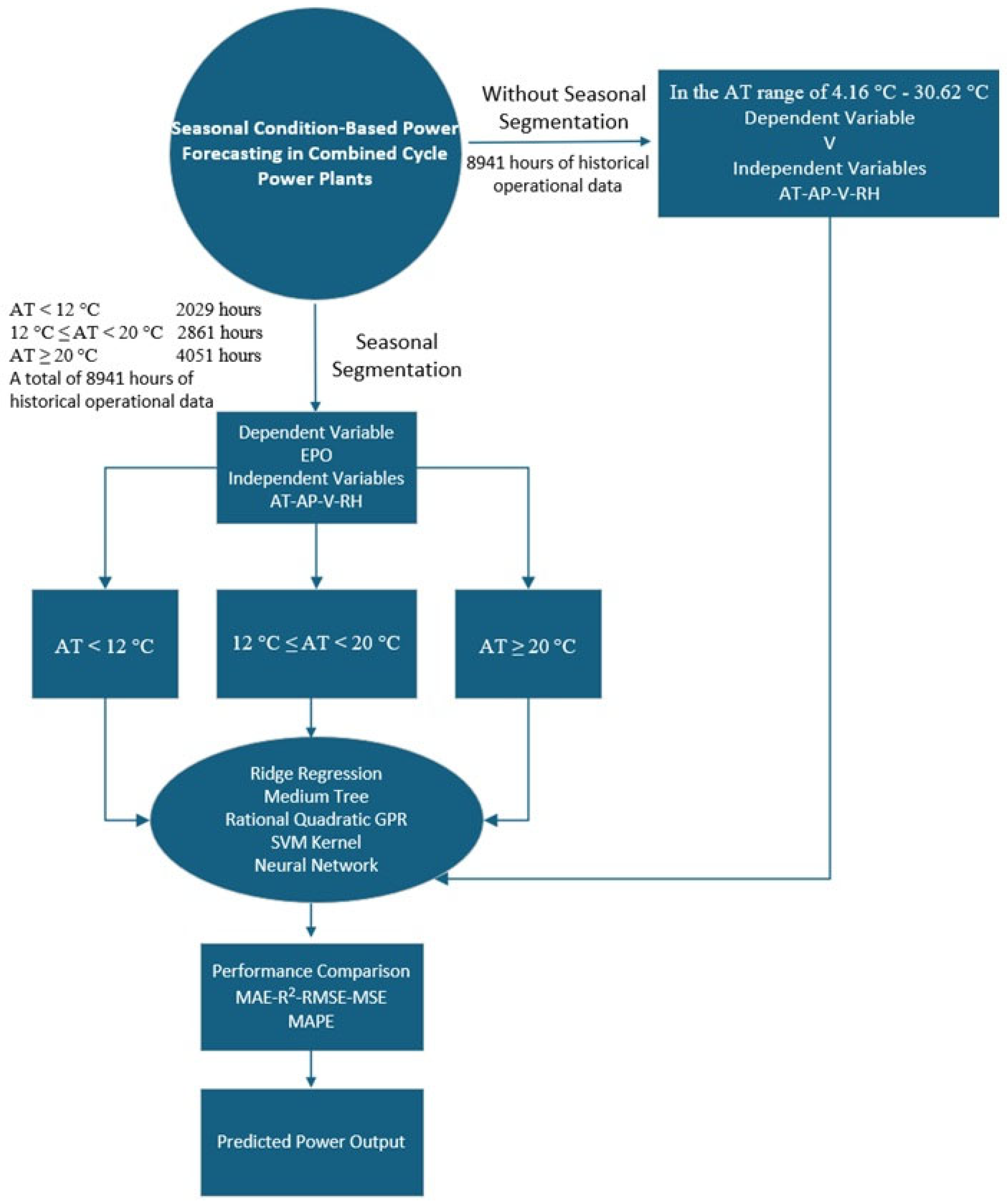
In this study, ambient conditions (AT, AP, and RH) and V were used as input variables, while EPO was defined as the target variable. Regression data were obtained from 8941 h of full-load actual operating records. Figure 2 presents the data flow diagram of the CCPP.
All variables in the dataset used in this study are defined below:
  • AT is an input variable with values ranging from 4.16 °C to 30.62 °C.
  • AP is an input variable with values ranging from 982.54 mbar to 1027.78 mbar.
  • RH is an input variable with values ranging from 24.61% to 100.00%.
  • V is an input variable with values ranging from 0.022 bara to 0.059 bara.
  • EPO is the target variable with values ranging from 860.30 MW to 950.56 MW.

3. Regression Methods

3.1. Ridge Regression

Regression analysis is one of the fundamental statistical approaches used to quantitatively examine the effect of various independent variables on a dependent variable [21]. Ridge Regression, on the other hand, is a special type of linear regression and is preferred to improve the predictive performance of the model and strengthen its generalization capability [22]. In particular, when there is a high correlation (multicollinearity) among the independent variables, the classical Ordinary Least Squares method produces unstable and unreliable estimates. Ridge Regression addresses this problem through the L2 regularization method. By adding a penalty term to the model coefficients, it constrains the magnitude of the coefficients, thereby reducing variance and improving the model’s generalization ability [23]. Moreover, this method reduces the risk of overfitting while achieving lower error rates on test data [24]. As a result, the model performs well not only on training data but also on real-world data. Ridge Regression provides much more stable results than classical methods, especially in high-dimensional datasets (where the number of features is large). Unlike some other regularization methods, Ridge Regression retains all variables in the model; that is, it does not shrink any variable’s effect to zero. This feature provides a particular advantage in application areas such as energy systems, where all inputs may contribute to the outcome to some extent.
Given a dataset with predicted values y ^ , independent variables X, coefficients β, actual values y, and a penalty parameter λ , the mathematical formulation of Ridge regression is as follows:
min β i = 1 n ( y i X i β ) 2 + λ j = 1 p β j 2
Here, i = 1 n y i X i β 2 represents the error term, while λ j = 1 p β j 2 denotes the penalty term.
In this study, the Ridge regression model was applied after standardizing all independent variables (AT, RH, V, and AP) such that they have a mean of zero and a variance of one. This preprocessing step ensured that the ridge penalty coefficient (λ) would be effective regardless of the original scales of the variables. Various λ values were tested in the model, and the optimal parameter was determined through automatic selection. In this analysis, the optimal λ value was found to be 0.1, which stabilized the coefficient estimates and enhanced the model’s generalization capability.

3.2. Regression Trees

The Classification and Regression Trees method, developed by Breiman and colleagues in 1984, stands out as an effective tool for analyzing large datasets. This method constructs a non-parametric tree structure that recursively partitions the data into more homogeneous subgroups by using a combination of explanatory variables (predictors), whether categorical or continuous. The primary objective is to best explain the variation in the target variable (response variable). As a result of this partitioning process, if the target variable is continuous, the model is referred to as a regression tree, whereas if the target variable is categorical, it is referred to as a classification tree [25].
A regression tree predicts the outcome y ^ for an input x by assigning it to a terminal node (leaf) based on the values of its predictors, and using the average of the response variable in that node as the prediction. This can be mathematically expressed as:
f ^ x = 1 N m i R m y i
where Rm is the region (leaf node) to which the input x is assigned, Nm is the number of observations in region Rm and y i is the observed value of the response variable for the i-th observation in that region.
A medium-sized DT is a model structured with limited depth to prevent the classical DT model from becoming overly complex. Compared to very shallow trees, this structure provides higher predictive power, while also significantly reducing the risk of overfitting that may occur in very deep trees. The term “Medium Tree” generally refers to DT configurations with predefined parameters such as a maximum depth and a minimum leaf size. In particular, with a structure where the minimum leaf size is set to 12, this model demonstrates high generalization ability and more robust performance against overfitting [26]. In this study, the minimum leaf size was set to 12.

3.3. Rational Quadratic GPR

Rational Quadratic GPR is a variant of the GPR method, distinguished by its capacity to model variations across multiple scales. GPR is a non-parametric, kernel-based probabilistic model that defines the distribution over functions using a mean and a covariance function. A Gaussian process can be formally described as:
m x = E f x , k x , x ı = C o v f x , f x ı
In practice, the mean function is typically assumed to be zero m x = 0 , and the learning is primarily governed by the kernel k x , x ı . The Rational Quadratic kernel is defined as:
k x , x ı = 1 + x x ı 2 2 l 2
where α is a positive parameter controlling the relative weighting of large- and small-scale variations and l is the characteristic length scale. The Rational Quadratic kernel can be interpreted as a scale mixture of squared exponential kernels with different length scales. This property allows the model to simultaneously capture both short-term fluctuations and long-term trends in the data [27]. GPR can be expressed as:
y = b ( x ) T β + f x , w i t h   f x ~ G P 0 , k x , x ı
where b ( x ) R p is a set of basis functions, β are regression weights, and the kernel k ( x , x ı θ ) is parameterized by hyperparameters θ . The training process involves estimating β , σ 2 (the noise variance), and θ , typically by maximizing the marginal likelihood.
Thanks to its flexibility, Rational Quadratic GPR performs particularly well on time series data exhibiting seasonal patterns, long-term drifts, and complex variability. Furthermore, it provides predictive variance estimates, allowing for the quantification of uncertainty in predictions. Being a non-parametric method, it does not assume any fixed functional form, which reduces the risk of overfitting—especially when working with small to medium-sized datasets [27,28,29].
In the model used in this study, a fixed basis function was adopted. The Rational Quadratic kernel was selected as the kernel function, aiming to flexibly capture variations occurring at different scales. Additionally, it was assumed that the kernel is isotropic, meaning it behaves uniformly in all directions. The kernel scale, signal standard deviation, and sigma values were automatically determined. This automatic adjustment enables the model to select the most appropriate parameters for the data. The input features were standardized to eliminate the influence of scale differences among variables. Furthermore, numerical parameter optimization was activated, allowing the model to reach optimal parameter values during the training process. These hyperparameter settings are intended to enhance both the accuracy and generalization capability of the model. In particular, they provide high flexibility and reliability in modeling nonlinear relationships within the data.

3.4. SVM Kernel

SVMs, based on Vapnik–Chervonenkis theory, are among the most widely used supervised learning methods in the field of ML due to their strong theoretical foundations. The SVM algorithm is a flexible and powerful method that produces effective results in both classification and regression problems. One of its most important advantages is the regularization property, which not only enables the model to learn from the training data but also allows it to exhibit high generalization capability when applied to previously unseen data.
An SVM is essentially a mathematical framework designed to maximize an objective function defined over a given dataset. In this context, the fundamental components of an SVM can be examined within four key concepts: separating hyperplane, maximum-margin hyperplane, soft margin, and kernel functions. The SVM algorithm aims to establish a decision boundary that provides the widest possible separation between classes by determining a maximum-margin hyperplane for linearly separable datasets. However, in practice, many datasets are not linearly separable. In such cases, it may be necessary to transform the data into a higher-dimensional feature space, at which point kernel functions come into play [30].
Kernel functions are mathematical tools that map samples from the original dataset into a higher-dimensional feature space. This transformation enables linearly inseparable samples to become linearly separable in the transformed space. The process is carried out using the kernel trick, which is one of the major advantages of SVMs. Through this technique, classification is made more efficient by performing inner product operations via kernel functions without explicitly transforming the data into higher dimensions [31]. Commonly used kernel functions in SVMs include linear, polynomial, radial basis function and sigmoid kernels [32]. These functions provide different advantages depending on the data structure and the type of problem.
m i n   1 2 w 2 + C i = 1 l ξ i + ξ i * s . t . y i w T Φ 𝔛 i b ε + ξ i y i + w T Φ 𝔛 i + b ε + ξ i * , i = 1,2 , . , l ξ i 0 , ξ i * 0
The final regression formula is as follows:
f x = i = 1 l a i a i * K x i , x + b
K x i , x j = e x p ( γ x i x j 2 ) , γ > 0
In this context, Φ ( x ) represents the nonlinear mapping function, w denotes the normal vector of the hyperplane, and b is the offset of the hyperplane. ε refers to the linear insensitive loss function. The expression, Φ x i ( x j ) corresponds to K ( x i x j ) , which is the kernel function satisfying the Mercer condition. The terms a i * and a i are the Lagrange multipliers in quadratic programming, while γ represents the parameter of the Gaussian radial basis kernel function.
In this study, the number of expansion dimensions parameter was automatically adjusted to ensure that the dimensionality of the transformed feature space was optimally selected with respect to the chosen kernel function. The regularization parameter (Lambda) was also determined automatically to prevent overfitting by controlling model complexity. Similarly, the kernel scale parameter was automatically selected and optimized to ensure balanced performance of the kernel function. The epsilon value, which defines the error tolerance in regression problems, was also set automatically, enabling the model to ignore small deviations and focus on more significant errors. Furthermore, data standardization was applied to bring all features onto the same scale, thereby allowing the SVM to learn more efficiently and stably. Finally, the iteration limit parameter was set to 1000, restricting the maximum number of iterations during the training process. All of these configurations were implemented to enhance the performance of the SVM model and to achieve a more generalizable structure.

3.5. Artificial Neural Network

Artificial Neural Networks (ANNs) were initially proposed with the aim of developing computer systems capable of mimicking the information processing mechanisms of the human brain. Today, ANNs have emerged as a powerful algorithmic framework widely used in various fields such as pattern recognition, prediction, and optimization. One of the most significant advantages of ANNs is their ability to learn from data and apply the acquired knowledge to previously unseen situations. Owing to these features, ANNs have become an effective tool for solving complex problems across many disciplines.
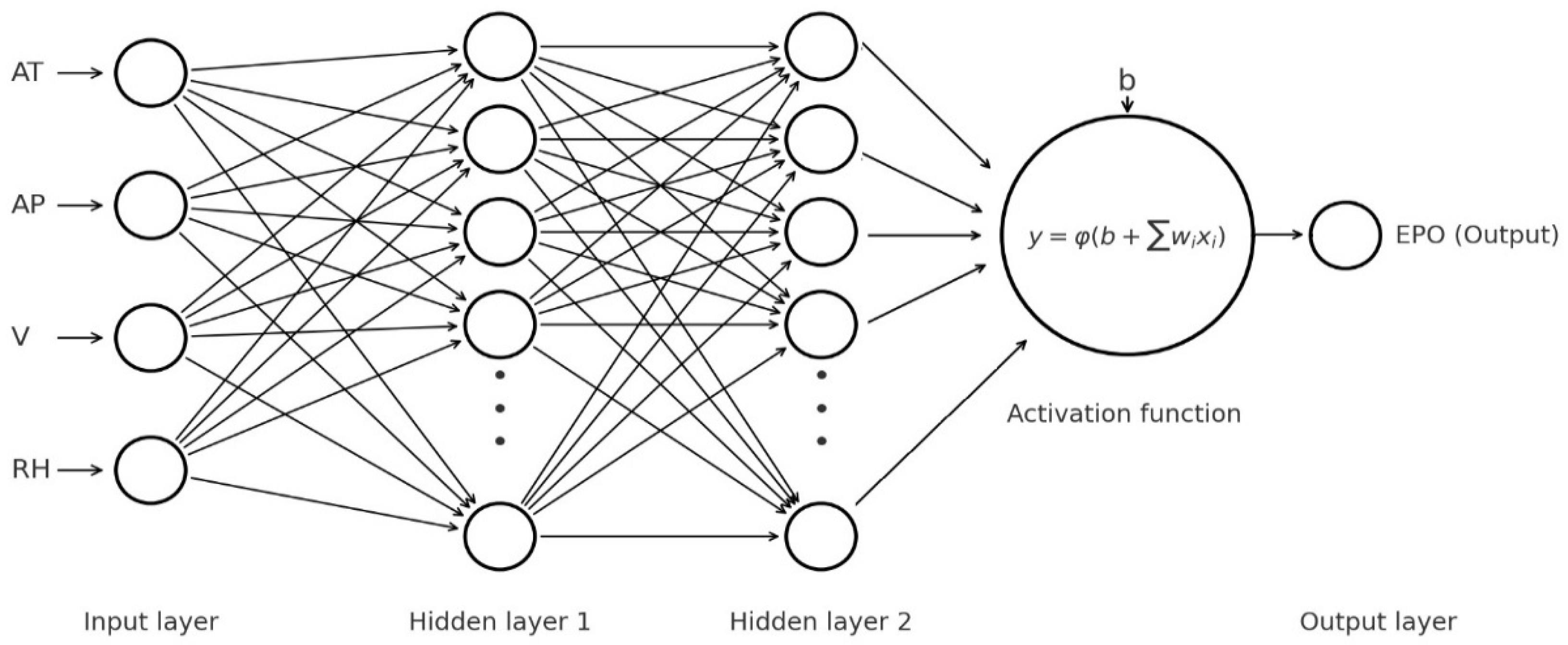
A typical ANN consists of three main structures: an input layer, one or more hidden layers, and an output layer. The operation of an ANN can be summarized as follows: (i) data are received by the input layer of the network and transferred to the first hidden layer; (ii) each neuron in a hidden layer performs a weighted operation on the inputs it receives, after which an activation function is applied to this output and the result is passed to the next layer; and (iii) this chain of operations continues until the output layer is reached, where the network produces its final output. This layered structure enables ANNs to achieve high levels of success in solving a wide variety of problems [33]. Figure 3 illustrates the architecture of the ANN model used in this study.
Mathematically, operations in an ANN can be expressed using weight matrices W(l), bias vectors b(l), and activation functions σ. For each layer l, the neurons are calculated as follows:
z l = W l a l 1 + b l
a l = σ z l
where a(l−1) represents the outputs of the previous layer and a(l) = x represents the initial input.
In this study, the ANN model was configured using the “Wide Neural Network” preset. The model consists of two fully connected layers: the first layer comprises 100 neurons, and the second layer comprises 10 neurons. The ReLU activation function was employed to enable the model to effectively capture nonlinear relationships within the data. During the training process, the maximum number of iterations was set to 1000. To reduce the risk of overfitting, the regularization parameter (Lambda) was set to zero. Furthermore, all input data were standardized to minimize the effects of scale differences across variables, allowing the model to process inputs more consistently. This configuration enables the ANN model to both learn complex patterns in the data and generate predictions with high accuracy.
When summarizing the advantages and limitations of the methods explained above, it is recognized that each has different strengths and weaknesses. Ridge Regression offers simplicity, interpretability, and robustness against overfitting through L2 regularization, but its linear nature restricts its ability to capture nonlinear relationships. DT provide intuitive, rule-based structures that are easy to interpret and can model nonlinear patterns; however, a single tree is prone to high variance and instability unless carefully pruned. GPR is particularly powerful for capturing complex, nonlinear relationships and providing prediction intervals that quantify uncertainty, yet it is computationally demanding for large datasets and highly sensitive to kernel selection. SVMs deliver strong generalization performance and resilience to outliers, especially with nonlinear kernels, but require careful tuning of hyperparameters such as C and γ, and may be computationally expensive. Finally, ANNs demonstrate superior performance in modeling high-dimensional and nonlinear data, especially with sufficient training data, though they often act as ‘black boxes’, require significant computational resources, and are vulnerable to overfitting unless regularization techniques are applied.

4. Performance Assessment

In order to evaluate the accuracy of the examined models, the prediction results were tested using the performance indicators listed below.

4.1. Coefficient of Determination (R2)

The R2 coefficient is one of the most frequently used indicators for evaluating the goodness of fit in linear models [34]. R2 measures how consistent the model’s predictions are with the actual values and reflects the proportion of the total variance in the target variable explained by the model. Its value ranges between 0 and 1; the closer it is to 1, the greater the explanatory power of the model. The formula for calculating R2 is given below [13,35]:
R 2 = 1 i = 1 N y i y i ^ 2 i = 1 N y i y ¯ 2
Here, N represents the number of samples. y i and y i ^ represent the actual and predicted values in the dataset, respectively. y ¯ is the mean of the actual values.

4.2. Mean Absolute Error (MAE)

To evaluate the accuracy and reliability of quantitative models, dimensional error metrics are commonly used in performance analysis, with MAE being one of the most widely applied [36]. MAE is the average of the absolute differences between the predicted values of a model and the actual values. Instead of squaring the differences, it calculates only the average of their absolute values. This metric reflects the model’s average prediction error and is less sensitive to large errors. The formula for calculating MAE is given below [13,14,16,35,37]:
M A E = i = 1 N y i y i ^ N  

4.3. Mean Square Error (MSE)

When the data follows a normal distribution, the MSE is a reliable and ideal method for evaluating the accuracy level of a model [38]. MSE is an error metric that represents the average of the squared differences between the predicted values and the actual values. MSE can be computed using the following formula [39,40]:
M S E = 1 N i = 1 N y i y i ^ 2

4.4. Root Mean-Squared Error (RMSE)

RMSE is a widely used metric for measuring the predictive accuracy of a model, representing the average magnitude of the error between the predicted and actual values [41]. The smaller the RMSE value, the closer the model’s predictions are to the actual values. The formula for calculating RMSE is given below [14,16,35,37]:
R M S E = i = 1 N y i y i ^ 2 N  

4.5. Mean Absolute Percentage Error (MAPE)

MAPE is a commonly used metric to evaluate the accuracy of a ML model. MAPE measures the average percentage difference between predicted and actual values. It is calculated using the following formula [13,14]:
M A P E = 1 N i = 1 N y i y i ^ y i × 100 %

4.6. Average Convergence Rate

The mean convergence indicates the average agreement between the predicted and measured EPO values, and it is calculated as follows:
A v e r a g e   C o n v e r g e n c e   R a t e % = 1 1 n i = 1 n y i y ^ i y ¯ × 100
Here, y i represents the measured EPO value, y ^ i denotes the predicted EPO, and y ¯ refers to the mean of the measured EPO values. This additional metric was used to present the prediction accuracy in a more interpretable way for power plant operators.

4.7. Forecast Evaluation Using Diebold–Mariano and Giacomini–White Tests

When comparing the performance of ML-based forecasting models, error metrics alone are not sufficient. It is also necessary to test whether the difference in predictive ability between models is statistically significant. For this purpose, the most commonly used methods in the literature are the Diebold–Mariano (DM) and Giacomini–White (GW) tests [42,43].
The DM test compares the forecast error series of two models. In this study, the predictive performances of the ANN and GPR models were compared. The forecast error series of the two models are defined as follows:
e t G P R = y t y ^ t G P R
e t A N N = y t y ^ t A N N
Loss farkı,
For MSE;
d t M S E = e t A N N 2 e t G P R 2  
For MAE;
d t M A E = e t A N N e t G P R
Test statistic:
D M = d ¯ 2 π f ^ d 0 T
Here, d ¯ denotes the mean of the loss differentials, T is the number of observations, and f ^ d 0 is the spectral density of the loss differential series at frequency zero, estimated using the Newey–West (HAC) estimator.
GW test evaluates conditional predictive performance. The loss differential series is regressed on a set of conditioning variables:
Regression model:
d t = α + u t  
Here, d t represents the loss differential between the two models, and α denotes the mean value of this differential.
Hypotheses:
H 0 : α = 0
H 1 : α 0
The Wald test statistic used to test these hypotheses is calculated as follows:
G W = α ^ V a r ^ α ^ 1 α ^
V a r ^ α ^ denotes the variance of the coefficient estimate. Under the null hypothesis H 0 : α = 0 , there is no significant difference in the conditional predictive performance between the two models. Under the alternative hypothesis H 1 : α 0 , a statistically significant difference exists between the models.

4.8. Bootstrap Method

The bootstrap method offers a powerful and flexible alternative for calculating prediction intervals in regression models. Unlike traditional parametric approaches, bootstrap eliminates the need for strict assumptions about the distribution of error terms. This approach derives the distribution of prediction errors directly from the observed data, enabling more reliable and accurate prediction intervals. It is particularly advantageous when the dataset is small or when the error distribution deviates from normality. To construct prediction intervals using bootstrap, the original dataset is resampled thousands of times, a regression model is fitted to each resampled dataset, and the prediction errors are computed. The percentile values of this error distribution are then used to form the final prediction intervals [44].
P I 1 α B o o t = [ y ^ i + q ~ α 2 , y ^ i + q ~ 1 α 2 ]
Here, y ^ i denotes the model prediction for the i-th observation, and q ~ α 2   a n d   q ~ 1 α 2 represent the lower and upper quantile values obtained through the bootstrap method, respectively.

5. Results

In this study, a total of 8941 h of actual full-load operation data obtained from the CCPP were used. An extrapolation analysis was conducted and performance evaluation was carried out using Linear Ridge, Medium Tree, Rational Quadratic GPR, SVM Kernel, and Neural Network algorithms. During the modeling process, the dataset was divided into 80% training and 20% testing subsets. In the first stage, analyses were performed on the general dataset covering all temperature values. Subsequently, the AT variable was divided into three sub-ranges based on seasonal distribution: AT < 12 °C, 12 °C ≤ AT < 20 °C, and AT ≥ 20 °C. In each temperature range, the performances of Linear Ridge, Medium Tree, Rational Quadratic GPR, SVM Kernel, and Neural Network methods were evaluated. In the final stage, the results of the seasonally segmented models were compared with those of the general model trained on the entire temperature range, and a comprehensive analysis was presented regarding the generalizability and accuracy of the models.
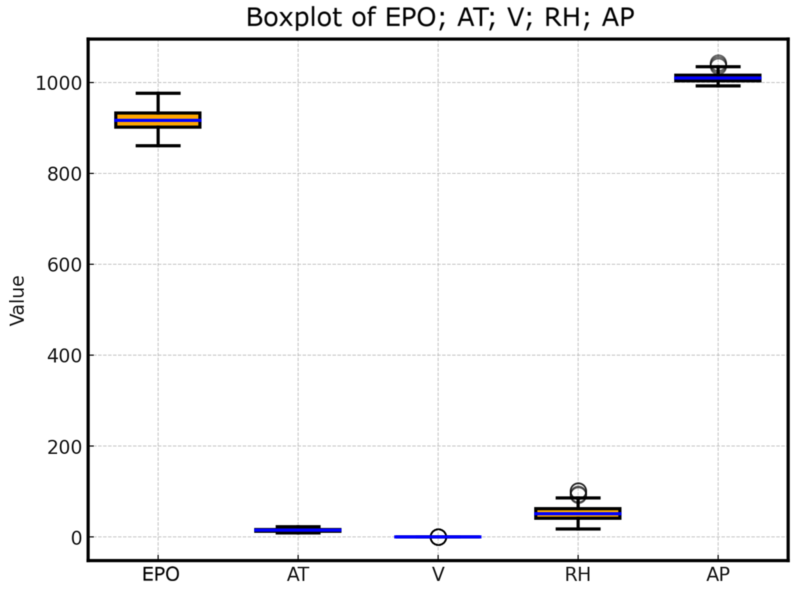
In this study, real-time operational data were used as the basis. The CCPP under investigation operates with a net output of 936 MW and a gross output of 950 MW. Its capability to operate at baseload makes the plant effective in providing primary and secondary frequency control services. The plant’s baseload capacity exhibits seasonal variability depending on environmental factors. The most significant cause of these fluctuations is AT; specifically, power generation decreases during the summer months while higher values are achieved in the winter. In addition, deteriorations in vacuum levels during the summer further exacerbate this reduction in power output. Such volatility in environmental variables leads to the presence of outliers in the dataset. Moreover, errors in data recording may occur due to faulty signals transmitted from measurement equipment, such as transmitters, to the DCS. For reliable results in regression analyses, it is crucial to identify and remove such outliers from the dataset. To this end, the box-plot method was applied, as presented in Figure 4. Following the filtering of outliers, the analyses were carried out on 8941 valid data points.
Table 1 presents the statistical information of the dataset. For each variable, the sample size is 8941, and the table includes the arithmetic mean and standard deviation values.
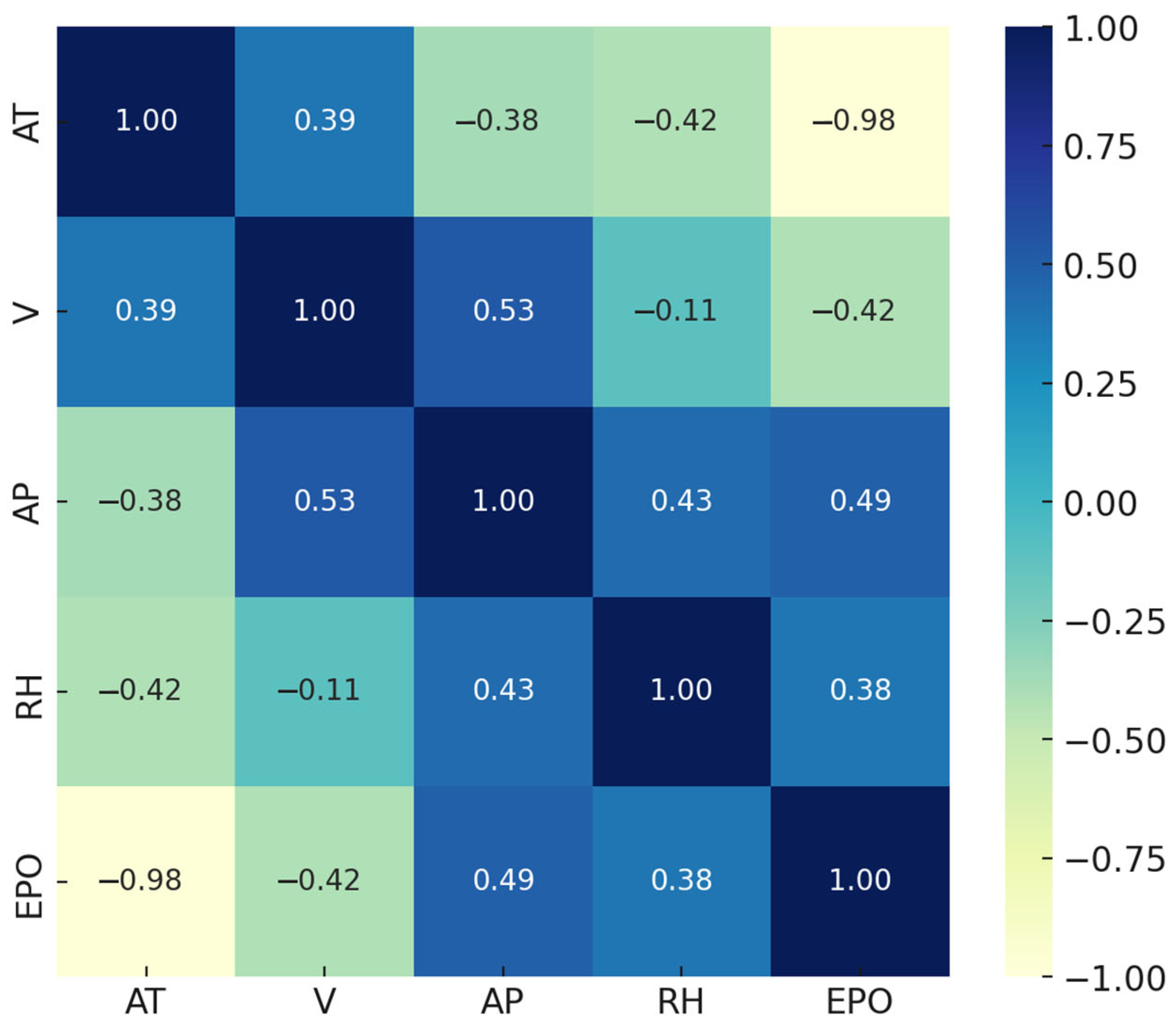
One of the fundamental tools used to detect the problem of multicollinearity is the correlation matrix. The correlation matrix presented in Figure 5 reveals the relationships of the independent variables both with each other and with the dependent variable, EPO. The closer the absolute value of the correlation coefficient between an independent variable and EPO is to 1, the stronger the linear relationship between them.
In this context, the correlation coefficient between AT and EPO was determined as −0.98. This very high and negative value clearly indicates that as AT increases, EPO tends to decrease, revealing a strong inverse relationship between the two variables. This can be explained by the fact that as temperature rises, the density of the air entering the GT decreases, which in turn reduces the generated power. On the other hand, the correlation coefficient between AP and EPO was calculated as 0.49. This value shows that AP has a positive effect on EPO; however, the strength of this relationship remains moderate. This indicates that as AP increases, air density also rises, which enhances the mass flow entering the turbine compressor and consequently increases EPO values. The correlation coefficient between RH and EPO, however, was found to be quite low. This suggests that RH does not have a significant impact on EPO and that their relationship is weak. For the V variable, the correlation coefficient with EPO was calculated as −0.42. This result indicates a negative and low-to-moderate relationship between increased V and reduced EPO. An increase in V raises the exhaust pressure of the ST, thereby limiting its net output power. Although this effect is not as pronounced as that of AT, the V parameter is still an important variable influencing plant performance. In conclusion, AT, AP, and V are seen as the primary operational variables determining output power in CCPPs. In contrast, the effect of RH remains limited and plays a secondary role.
Overall, the results of the correlation matrix reveal the dominant and decisive effect of AT on EPO. Based on this, in the present study, the dependent variable—EPO—was modeled by segmenting the most correlated variable, AT, into seasonal temperature ranges, and the improving effect of this segmentation on the prediction model was evaluated.

5.1. Findings of Regression Analysis on the Entire Dataset

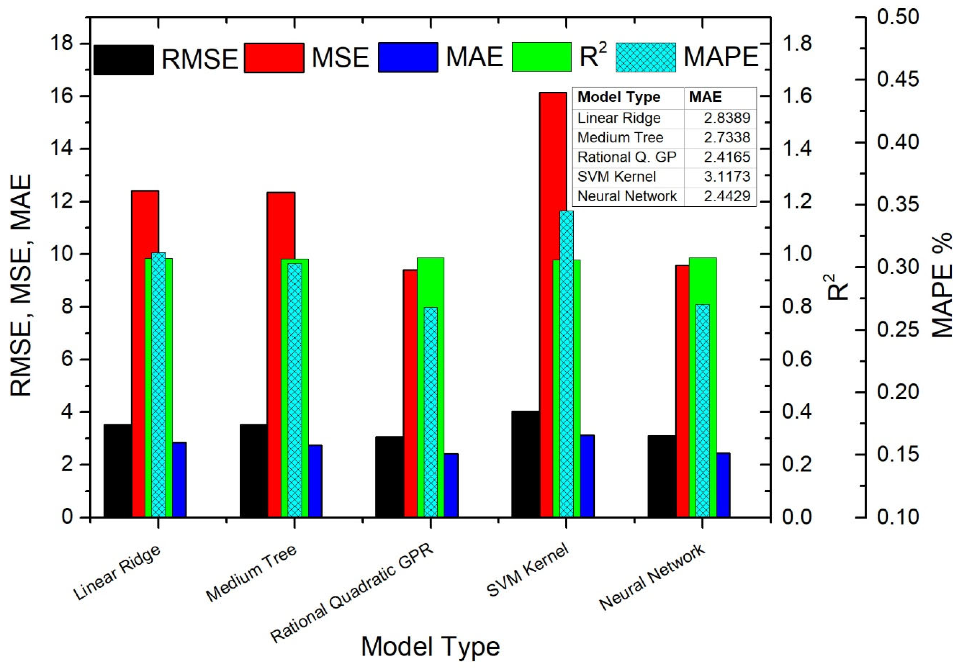
The results of the regression analyses conducted without seasonal segmentation of the temperature data are presented in Figure 6. The figure presents a performance comparison of five different ML models: Linear Ridge, Medium Tree, Rational Quadratic GPR, SVM Kernel, and Neural Network. The comparison was carried out using four statistical metrics: RMSE, MSE, MAE, R2 and MAPE. According to the results, the Rational Quadratic GPR model yielded the lowest error value (MAE = 2.4165), indicating the highest prediction accuracy. In contrast, the model with the highest error was the SVM Kernel (MAE = 3.1173). The Neural Network demonstrated competitive performance with relatively low error values (MAE = 2.4429). Overall, ensemble and non-linear methods (Rational Quadratic GPR, Neural Network) provided higher accuracy and reliability compared to linear models (Linear Ridge). Furthermore, the higher R2 values of these models indicate that they were more successful in capturing the complex non-linear behavior of the system.

5.2. Findings of Regression Analysis Based on Seasonal Temperature Ranges (AT < 12 °C, 12 °C ≤ AT < 20 °C, and AT ≥ 20 °C)

In the technical manuals of turbine manufacturers, characteristic curves are provided to show the effects of ambient conditions on EPO. The main reason for this is that environmental parameters directly influence turbine performance. However, due to natural performance losses (degradation) occurring in turbines during operation, the effect coefficients provided in these manuals may change over time. In this study, using approximately five years of real operational data, the aim was to predict EPO with the highest possible accuracy, and among the four independent variables examined (AT, AP, RH, V), AT was identified as the most dominant parameter.
In load forecasting for CCPPs, it is often assumed that there is a fixed power reduction for every 1 °C increase in temperature. However, this approach overlooks the varying impact of temperature across different ranges. Therefore, in this study, to improve prediction accuracy, AT was analyzed across three different temperature ranges. The results of the analysis revealed that the effect of a 1 °C increase in temperature on EPO varies depending on factors such as changes in air density, the temperature dependence of compressor–turbine efficiencies, the contribution of GT exhaust temperature to HRSG steam production, the effect of V in the ST, and operational control limits. Hence, instead of explaining the relationship between AT and EPO with a fixed coefficient, piecewise linear (segment-based) modeling provides more realistic results.
When the entire temperature range (4.16 °C–30.62 °C) is considered as a whole, the Ridge regression coefficients indicate that each 1 °C increase in AT leads to an average decrease of 3.96 MW in EPO. However, segment-based analyses revealed that this effect varies across temperature ranges: for AT < 12 °C, each 1 °C increase results in a decrease of approximately 2.80 MW in PE; for 12 °C ≤ AT < 20 °C, the decrease is approximately 4.13 MW; and for AT ≥ 20 °C, the decrease is approximately 3.72 MW. These findings demonstrate that while the effect of AT on EPO is linear, it occurs with different slopes across different temperature ranges, indicating that the assumption of a fixed coefficient is insufficient.
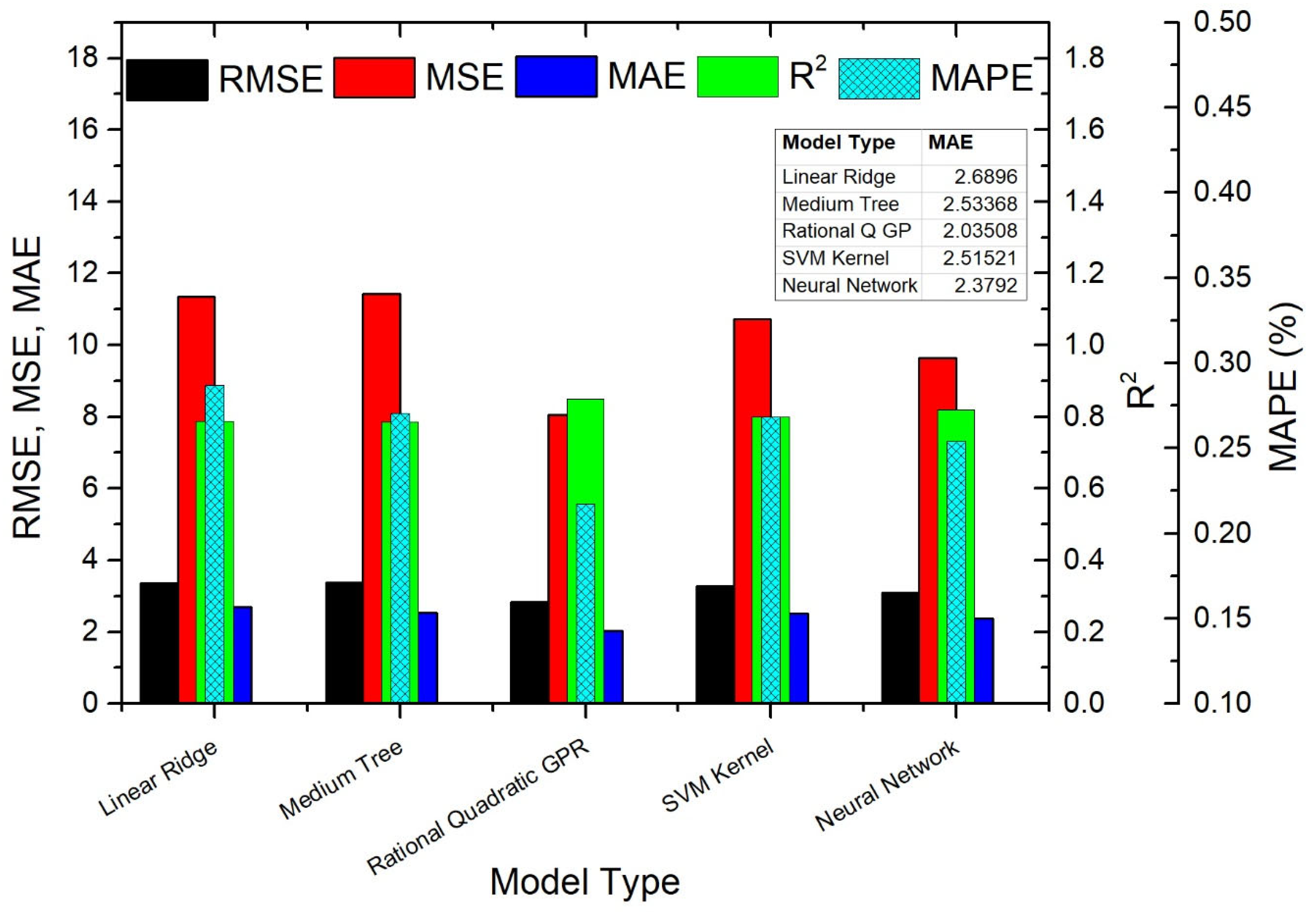
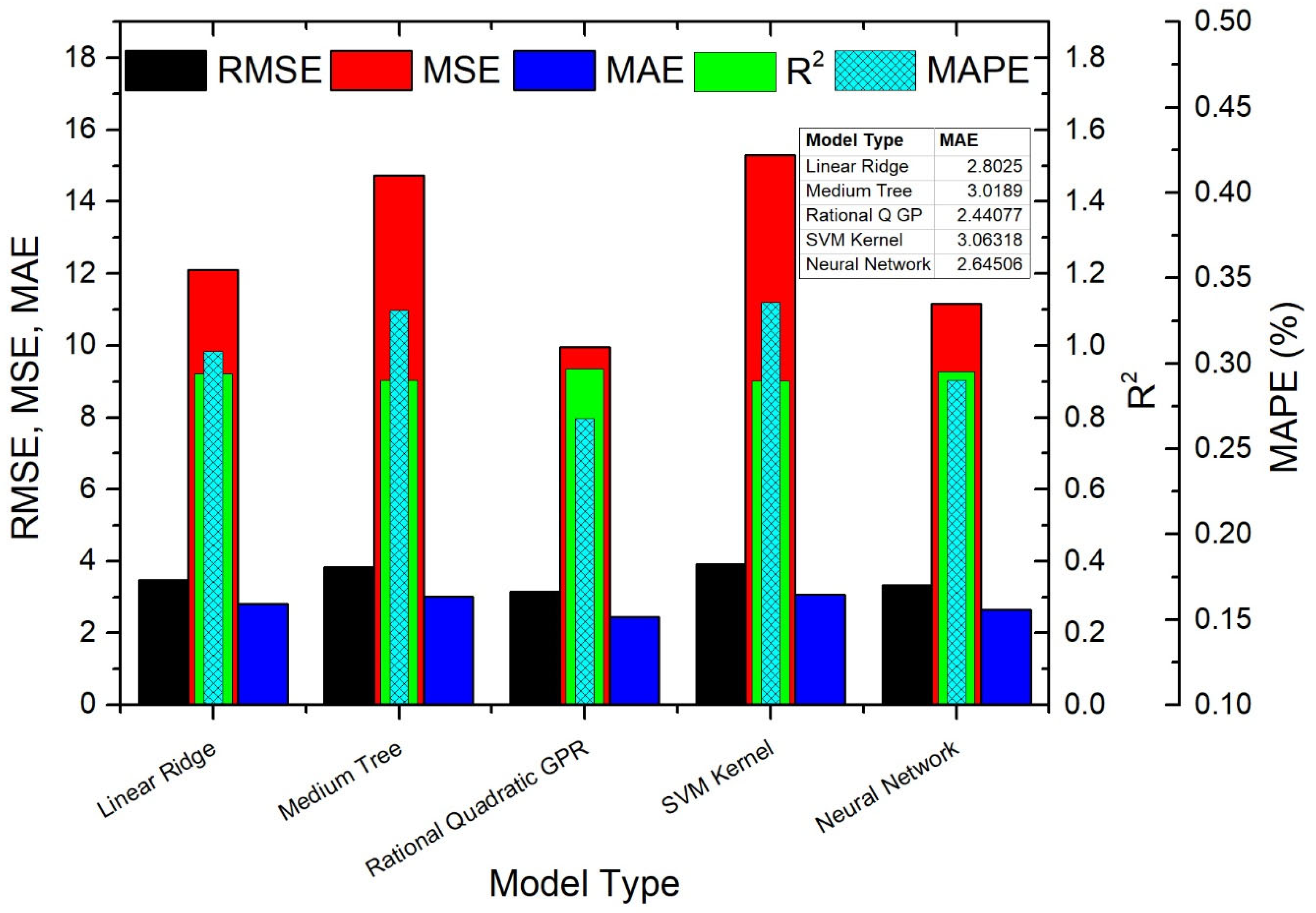
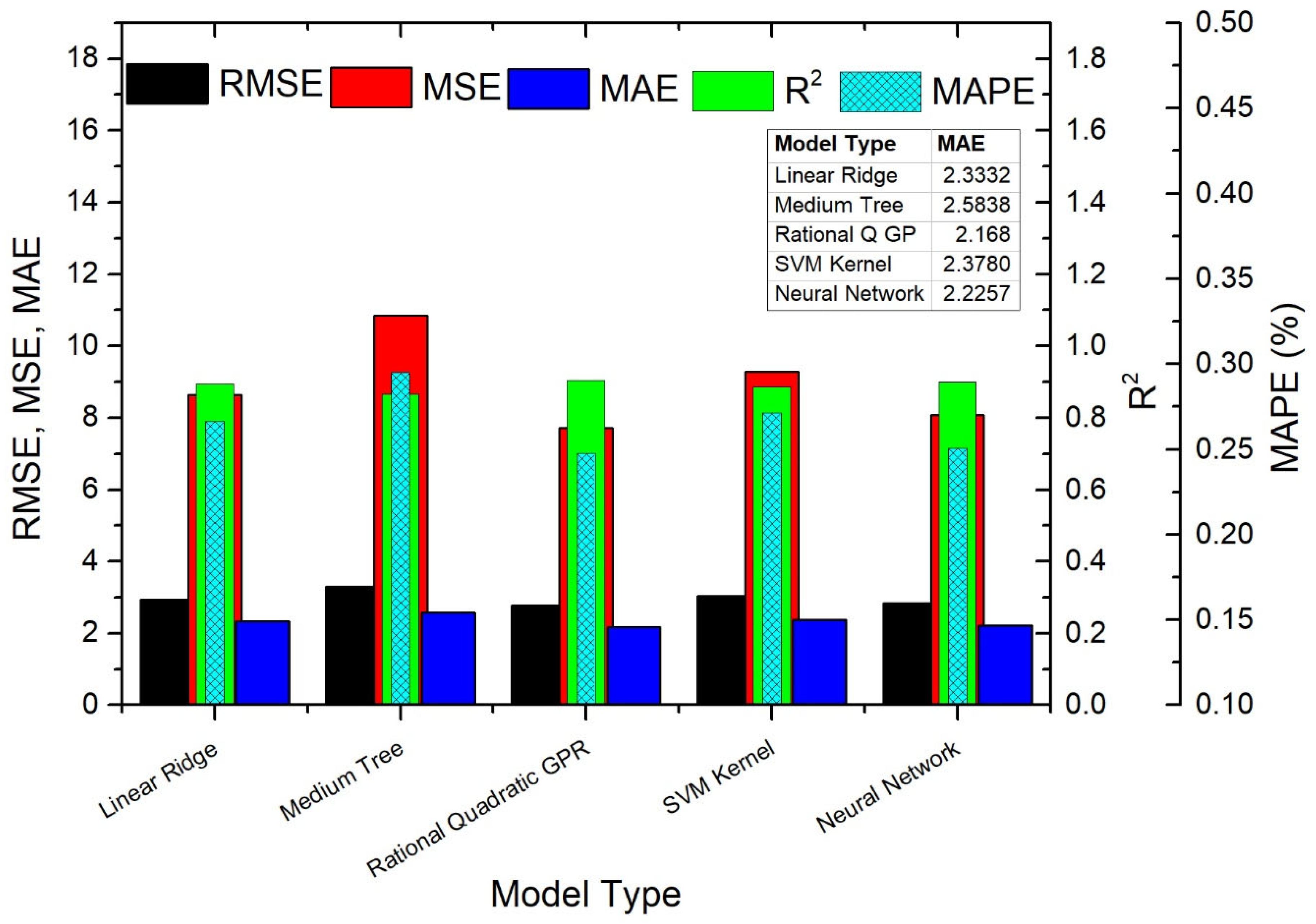
When comparing the performances of the Linear Ridge, Medium Tree, Rational Quadratic GPR, SVM Kernel, and Neural Network models, it was observed that the highest accuracy was achieved with the Rational Quadratic GPR model. Figure 7, Figure 8 and Figure 9 present the comparisons of all models according to seasonal conditions. In the AT < 12 °C range, the Rational Quadratic GPR model achieved MAE = 2.03508, demonstrating the best predictive accuracy. The SVM Kernel (MAE = 2.51521) also exhibited similarly strong performance. However, the Linear Ridge model produced the highest error (MAE = 2.6896), making it weaker compared to the other models. The Neural Network (MAE = 2.3792) and Medium Tree (MAE = 2.53368) showed intermediate performance (Figure 7). In the 12 °C ≤ AT < 20 °C range, the Rational Quadratic GPR model again provided the most accurate predictions (MAE = 2.44077). The Linear Ridge (MAE = 2.8025) and Neural Network (MAE = 2.64506) achieved moderate accuracy, while the Medium Tree (MAE = 3.0189) and SVM Kernel (MAE = 3.06318) recorded the highest error values, indicating weaker performance compared to the other models (Figure 8). In the AT ≥ 20 °C range, the lowest error was obtained with the Rational Quadratic GPR model (MAE = 2.168), which showed the highest predictive accuracy. The Neural Network (MAE = 2.2257) delivered a closely competitive performance. The Linear Ridge (MAE = 2.3332) and SVM Kernel (MAE = 2.3780) achieved moderate accuracy, while the Medium Tree produced the highest error (MAE = 2.5838), making it the weakest performer among the models (Figure 9).
According to the analysis of approximately 8941 h of full-load operation data, 2029 h occurred in the AT < 12 °C range, 2861 h in the 12 °C ≤ AT < 20 °C range, and 4051 h in the AT ≥ 20 °C range. This distribution indicates that a significant portion of the plant’s operating time took place under high-temperature conditions. Considering the segmentation by temperature ranges, the prediction models were separately optimized for each range using the Rational Quadratic GPR model, and the weighted average MAE value was obtained as 2.225. In contrast, when all data were evaluated without segmentation, the MAE value obtained with the same model remained at 2.417. This comparison clearly demonstrates that temperature-based segmentation significantly improves prediction accuracy and thereby contributes to operational efficiency.
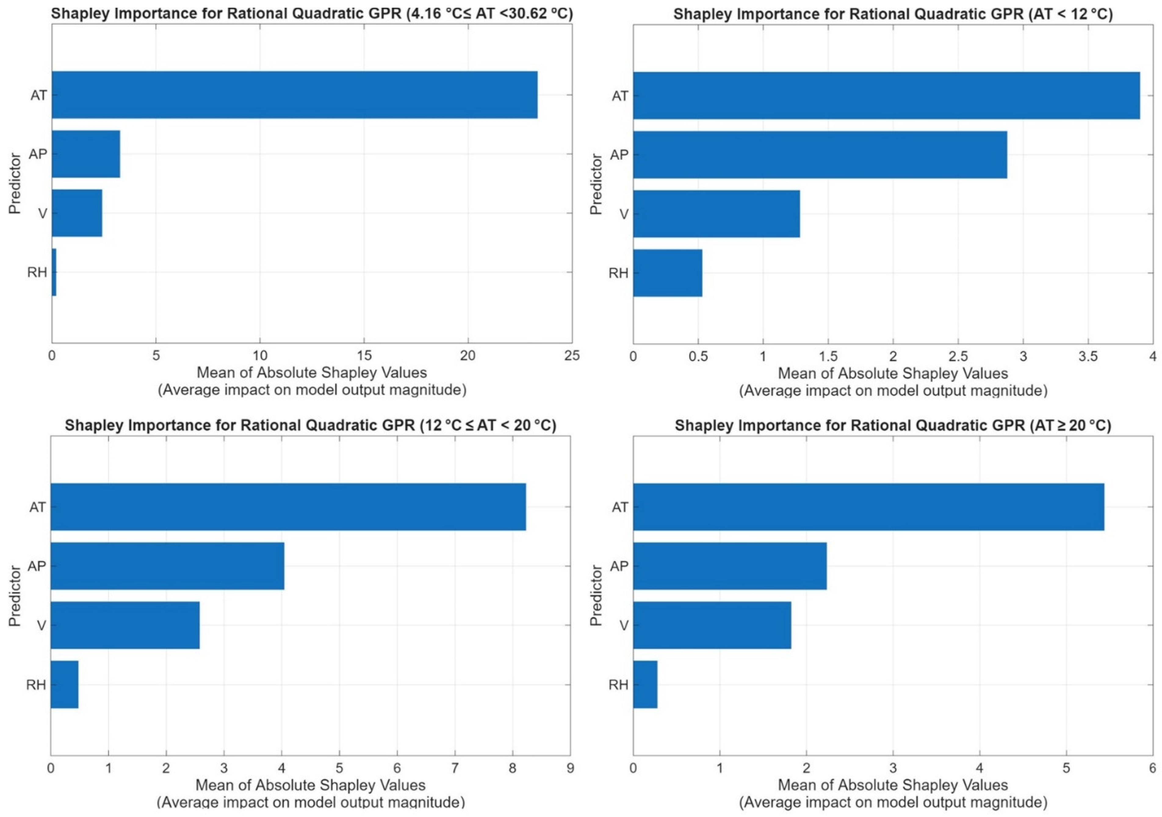
In Figure 10, Shapley importance plots are presented for the global Rational Quadratic GPR model (top left) and the three temperature-segmented models. In all models, AT remains the most influential predictor, confirming its dominant impact on EPO. AP and V are the next most significant features, though their relative contributions shift slightly across temperature ranges: AP has a stronger effect in colder regimes (AT < 12 °C), whereas V becomes slightly more influential at higher temperatures (AT ≥ 20 °C). RH consistently shows minimal impact. Temperature-based segmentation thus produces models with feature importances that more accurately reflect the physical sensitivities of the plant under each regime, reducing cross-regime mismatches and improving interpretability. Figure 10 clearly shows that temperature segmentation allows the model to differentiate how AP and V influence EPO under different thermal conditions. For example, in colder regimes, AP exhibits a larger positive contribution to output prediction, consistent with the higher density of intake air improving turbine performance. Conversely, in warmer regimes, V gains relative importance as condenser performance becomes more critical for overall plant efficiency. These findings confirm that segmentation not only improves statistical accuracy but also leads to more physically consistent insights, aligning the model’s behavior with thermodynamic expectations.
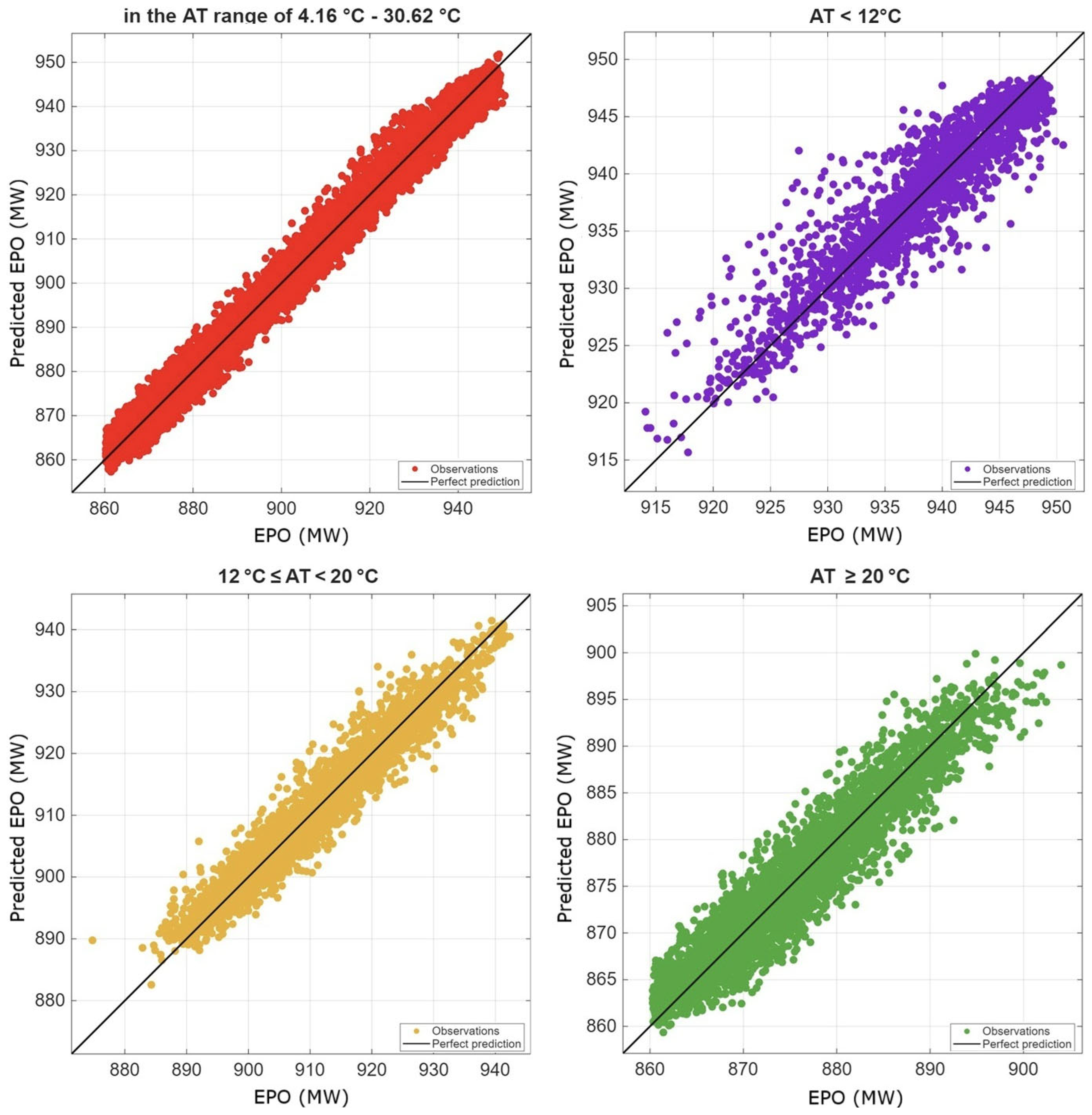
Figure 11 shows the comparison between the predicted EPO obtained from the Rational Quadratic GPR model and the actual measured values across different AT ranges. In the segment-based evaluation, the AT < 12 °C range stood out with the lowest error value (MAE = 2.035), indicating that the model was able to generate predictions closest to the actual values under cold weather conditions. On the other hand, the high R2 obtained in the 12–20 °C range (R2 = 0.935) reveals that in this segment, the model achieved the best alignment of predictions with the overall trend.
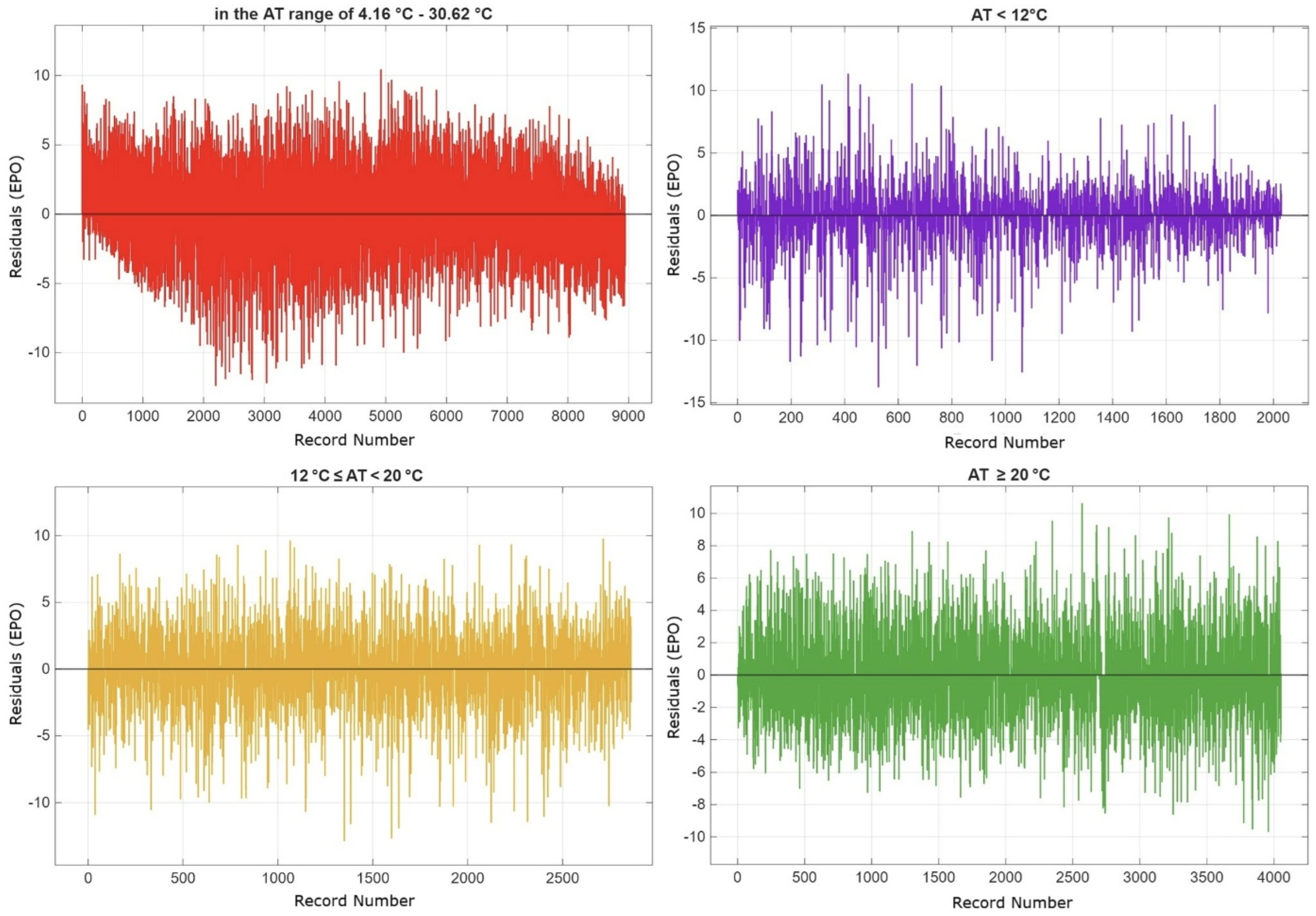
Figure 12 presents the residual distributions (differences between actual and predicted values) of the models developed with seasonal temperature segmentation (AT < 12 °C, 12 °C ≤ AT < 20 °C, and AT ≥ 20 °C) using the Rational Quadratic GPR model, compared with the general model constructed without segmentation. The findings indicate that the residuals of the models developed for low and high temperature ranges are clustered within narrower intervals and that systematic biases are minimized. This demonstrates that segment-based modeling provides more stable performance, particularly under extreme temperature conditions. On the other hand, the residual distribution of the general model developed without temperature segmentation shows high variance and contains noticeable systematic errors. This comparison clearly highlights that the temperature-based modeling approach plays a critical role in improving prediction accuracy and ensuring operational reliability.
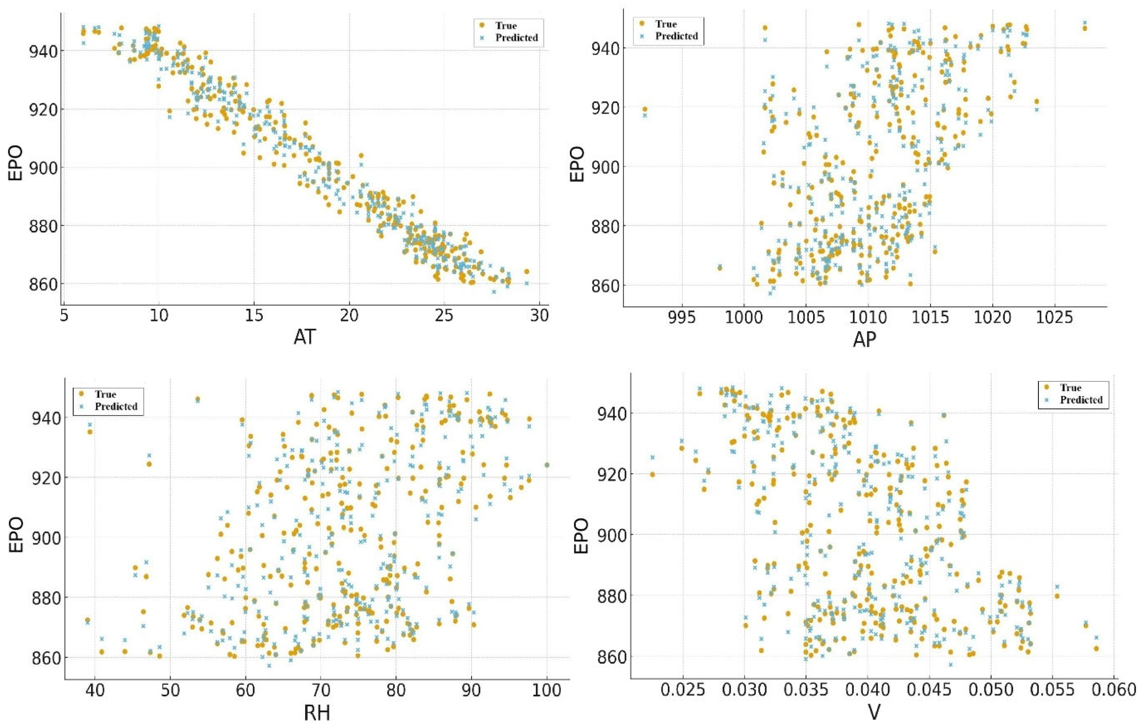
Figure 13 illustrates the relationship between the EPO of the CCPP and four key environmental variables (AT–AP, RH, and V) using the ANN method across the entire temperature range (4.16 °C–30.62 °C). The scatter plots include both the actual (True) and predicted (Predicted) values, allowing a direct comparison of the model’s predictive performance. Overall, the close distribution of actual and predicted values for all variables demonstrates that the applied model successfully captured the impact of environmental variables on plant performance.
In this study, the predictive performance of ANN and GPR models was compared. To statistically evaluate the differences in model accuracy, the DM and GW tests were applied. According to the DM test results, the mean squared error differences between the two models were found to be significantly different (statistic = 7.8491, p < 0.0001). Similarly, the GW test revealed that the correlation between the prediction errors was statistically significant (statistic = 74.5780, p < 0.0001). The results of both tests indicate that the GPR model provides more consistent and accurate predictions compared to the ANN model. These findings support the preference for the GPR model in regression problems.
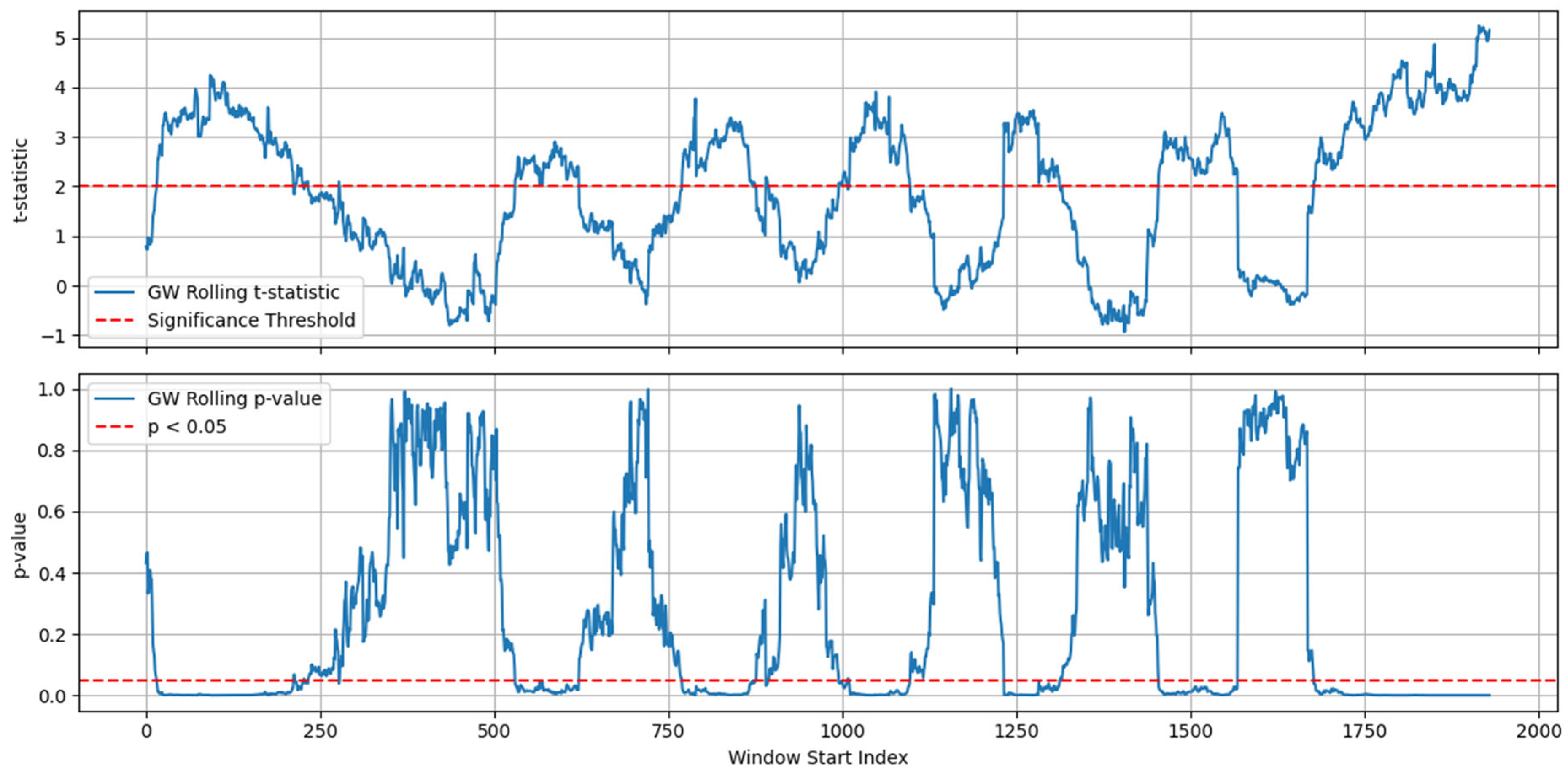
Furthermore, to examine how the predictive accuracy of the ANN and GPR models changes over time, a rolling-window GW test was applied. Figure 14 presents the rolling-window GW test results. Using rolling windows of 100 observations each, the differences in the squared prediction errors were statistically tested for every period. The resulting t-statistic curve reveals that the GPR model significantly outperforms the ANN model during certain periods, while the performance gap narrows in others. This fluctuation indicates that the models’ accuracy does not remain constant over time and varies depending on conditions. Moreover, the fact that the p-values fall below 0.05 in many windows statistically confirms that the GPR model is not only superior on average but also outperforms the ANN model during specific periods. This finding suggests that the GPR model can provide more reliable predictions in dynamic data environments.
In addition, for the GPR model, Bootstrap-based prediction intervals (B = 2000) at the 95% confidence level were calculated and evaluated using appropriate metrics such as coverage probability, mean interval width, and the Winkler score. The results show that the prediction intervals obtained through the bootstrap method are very close to the targeted 95% coverage probability (approximately 94.97%), while providing a narrow mean width (around 11.73 MW) (Table 2). The Winkler and Interval scores are low, indicating that the intervals are successful in terms of both coverage and sharpness.
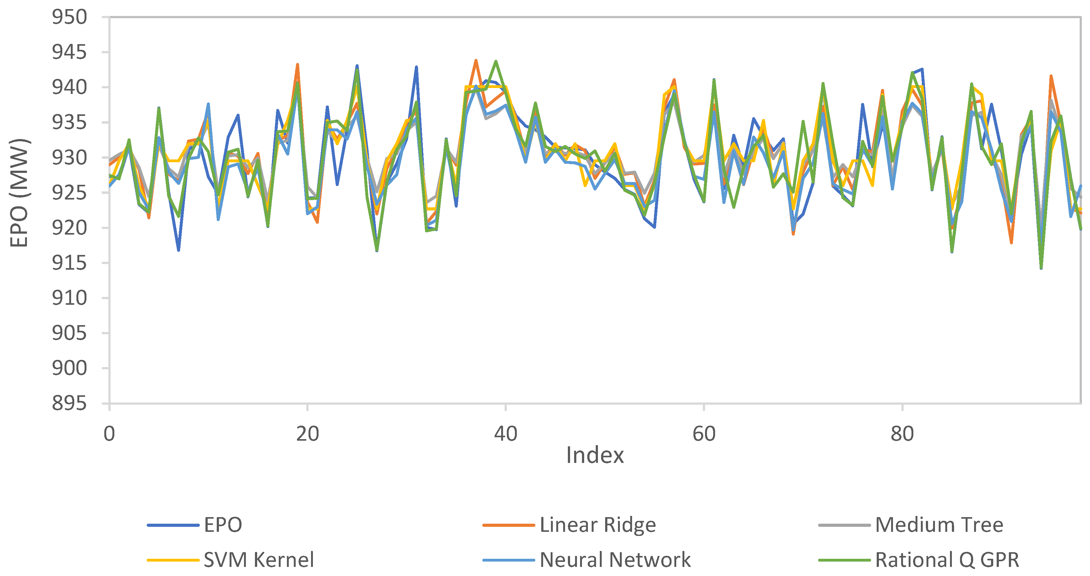
Figure 15 the performances of five different models used to predict EPO are compared. The graph was prepared for conditions where AT < 12 °C. As can be seen, all models successfully captured the overall trend and produced predictions quite close to the actual values. However, the Rational Quadratic GPR model was found to reflect the fluctuations more accurately and to achieve the closest fit to the actual values.
In conclusion, the seasonal temperature segmentation analyses conducted in this study revealed that environmental conditions have a decisive impact on the accuracy of power generation forecasting in CCPPs. The approaches developed by incorporating seasonal variations into the model optimized prediction performance across different temperature ranges. This improvement in short-term load forecasting contributed to more efficient management of fuel consumption, more reliable production planning, and the reduction of economic losses arising from supply–demand imbalances in intraday markets. Thus, by modeling seasonal variability, operational efficiency was sustainably enhanced.

6. Discussion

The temperature-based segmentation approach developed in this study enabled more accurate prediction of EPO in CCPPs and significantly reduced the error compared to predictions made with a single model. In particular, segmentation based on AT led to a notable improvement in model accuracy, demonstrating that considering temperature ranges separately is a critical factor for enhancing prediction performance.
The significance of this improvement becomes clearer when considering that natural gas CCPPs operate at full load for thousands of hours throughout the year. Prediction errors accumulated over such long operating periods can lead to system imbalances and economic losses. In this context, the achieved increase in accuracy is not merely a numerical success, but also a tangible contribution to operating the system more reliably, stably, and efficiently. With more accurate EPO predictions, errors in load forecasting for day-ahead and intraday markets are reduced, supply–demand imbalances are minimized, and the associated penalty costs are lowered.
A review of the literature reveals that no study has reported such a low weighted average MAE value for a power plant of this scale. This result demonstrates that the dataset was carefully prepared; time intervals in which secondary and primary frequency control were applied in the turbines were thoroughly examined, sensor errors were filtered out, and natural variations in baseload levels between summer and winter were distinguished from faulty data.
The improvement achieved not only enhances prediction accuracy, but also contributes to more effective natural gas supply planning, fuel optimization, and production strategies. In many cases, such forecasting improvements provide greater economic benefits than direct revenue increases by generating indirect operational efficiency gains. Therefore, the proposed method can be regarded as a practical decision-support tool applicable to similar natural gas power plants and can contribute to enhancing sustainability and market alignment within the energy system.
However, this study has certain limitations. The models were trained solely on data collected from a single CCPP. In future work, similar analyses are planned to be carried out under different geographical and climatic conditions, and the need for recalibration of the temperature segmentations will be assessed. Such analyses will enhance the generalizability of the proposed approach and contribute to its broader applicability in the literature.

7. Conclusions

This study was conducted to accurately predict the full-load EPO of CCPPs under environmental conditions and operational parameters, by utilizing real-time operational data and advanced ML-based forecasting models. Four key variables affecting power output (AT, AP, RH, and V) were analyzed in detail.
The initial modeling process was carried out using approximately 8941 h of full-load data and was performed on the entire dataset without applying temperature segmentation. Correlation analyses revealed that AT is the most influential variable on EPO, with a strong negative relationship. This finding highlighted the necessity of considering temperature as a separate parameter in the modeling process.
Accordingly, the dataset was divided into three different temperature ranges (AT < 12 °C, 12 °C ≤ AT < 20 °C, and AT ≥ 20 °C), and separate models were developed for each segment. Among the methods applied for power prediction, the Rational Quadratic GPR model exhibited higher accuracy in all scenarios compared to other approaches. While the MAE value was 2.417 MW in the non-segmented model, it was calculated as 2.035 MW, 2.441 MW, and 2.168 MW for the segmented models, respectively. With this approach, the weighted average MAE value was reduced to 2.225 MW, providing an improvement in accuracy of 192 kW. The average convergence rate of the predicted power output values to the actual values reached 99.77%.
The results demonstrate that this improvement in accuracy, achieved in plants operating thousands of hours annually, creates operational and economic value by reducing production-demand imbalances and the associated penalty costs. Furthermore, the study proves that data-driven and temperature-segmentation-based models can be effectively applied to different power plants with appropriate calibrations.
In conclusion, this study fills an important gap in the literature and demonstrates that temperature-based segmentation is not merely a statistical improvement, but also a practical strategy for enhancing the technical and economic performance of CCPPs. The findings provide a foundation for future studies involving the inclusion of additional environmental variables, the analysis of different load regimes, and the evaluation of the method under various market conditions, thereby further strengthening its effectiveness and generalizability.

Author Contributions

Conceptualization, A.A.; data curation, A.O.B.; formal analysis, A.A. and A.O.B.; investigation, A.A. and A.O.B.; methodology, A.A. and A.O.B.; visualization, A.O.B.; writing—original draft, A.A. and A.O.B.; writing—review and editing, A.A. and A.O.B. All authors have read and agreed to the published version of the manuscript.

Funding

This research received no external funding.

Data Availability Statement

The raw data supporting the conclusions of this article will be made available by the authors on request. The data are not publicly available due to commercial confidentiality.

Conflicts of Interest

Author Ali Osman Büyükköse was employed by the company Enerjisa Enerji Uretim Inc. The remaining authors declare that the research was conducted in the absence of any commercial or financial relationships that could be construed as a potential conflict of interest.

List of Abbreviations

ANNArtificial Neural Network
APAtmospheric Pressure
ATAmbient Temperature
CCPPCombined Cycle Power Plant
DCSDistributed Control System
DMDiebold–Mariano
DNNDeep Neural Network
DTDecision Tree
EPOElectrical Power Output
GPRGaussian Process Regression
GTGas Turbine
GWGiacomini–White
HRSGHeat Recovery Steam Generator
MAEMean Absolute Error
MAPEMean Absolute Percentage Error
MLMachine Learning
MSEMean Square Error
R2Coefficient of Determination
RHRelative Humidity
RMSERoot Mean Square Error
STSteam Turbine
SVMSupport Vector Machine
VCondenser Vacuum

References

  1. International Energy Agency (IEA). 2025. Available online: www.iea.org (accessed on 1 August 2025).
  2. López Hernández, O.; Romero Romero, D.; Badaoui, M. Economic Dispatch of Combined Cycle Power Plant: A Mixed-Integer Programming Approach. Processes 2024, 12, 1199. [Google Scholar] [CrossRef]
  3. Yi, Q.; Xiong, H.; Wang, D. Predicting power generation from a combined cycle power plant using transformer encoders with DNN. Electronics 2023, 12, 2431. [Google Scholar] [CrossRef]
  4. Kotowicz, J.; Brzęczek, M. Analysis of increasing efficiency of modern combined cycle power plant: A case study. Energy 2018, 153, 90–99. [Google Scholar] [CrossRef]
  5. Surase, R.S.; Konijeti, R.; Chopade, R.P. Thermal performance analysis of gas turbine power plant using soft computing techniques: A review. Eng. Appl. Comput. Fluid Mech. 2024, 18, 2374317. [Google Scholar] [CrossRef]
  6. Mattos, H.A.D.S.; Bringhenti, C.; Cavalca, D.F.; Silva, O.F.R.; Campos, G.B.D.; Tomita, J.T. Combined cycle performance evaluation and dynamic response simulation. J. Aerosp. Technol. Manag. 2016, 8, 491–497. [Google Scholar] [CrossRef]
  7. Arferiandi, Y.D.; Caesarendra, W.; Nugraha, H. Heat rate prediction of combined cycle power plant using an artificial neural network (ANN) method. Sensors 2021, 21, 1022. [Google Scholar] [CrossRef] [PubMed]
  8. Siddiqui, R.; Anwar, H.; Ullah, F.; Ullah, R.; Rehman, M.A.; Jan, N.; Zaman, F. Power prediction of combined cycle power plant (CCPP) using machine learning algorithm-based paradigm. Wirel. Commun. Mob. Comput. 2021, 2021, 9966395. [Google Scholar] [CrossRef]
  9. Lobo, J.L.; Ballesteros, I.; Oregi, I.; Del Ser, J.; Salcedo-Sanz, S. Stream learning in energy IoT systems: A case study in combined cycle power plants. Energies 2020, 13, 740. [Google Scholar] [CrossRef]
  10. Castillo, A. Risk analysis and management in power outage and restoration: A literature survey. Electr. Power Syst. Res. 2014, 107, 9–15. [Google Scholar] [CrossRef]
  11. Kesgin, U.; Heperkan, H. Simulation of thermodynamic systems using soft computing techniques. Int. J. Energy Res. 2005, 29, 581–611. [Google Scholar] [CrossRef]
  12. Pachauri, N.; Ahn, C.W. Electrical energy prediction of combined cycle power plant using gradient boosted generalized additive model. IEEE Access 2022, 10, 24566–24577. [Google Scholar] [CrossRef]
  13. Afzal, A.; Alshahrani, S.; Alrobaian, A.; Buradi, A.; Khan, S.A. Power plant energy predictions based on thermal factors using ridge and support vector regressor algorithms. Energies 2021, 14, 7254. [Google Scholar] [CrossRef]
  14. Qu, Z.; Xu, J.; Wang, Z.; Chi, R.; Liu, H. Prediction of electricity generation from a combined cycle power plant based on a stacking ensemble and its hyperparameter optimization with a grid-search method. Energy 2021, 227, 120309. [Google Scholar] [CrossRef]
  15. Sun, L.; Liu, T.; Xie, Y.; Zhang, D.; Xia, X. Real-time power prediction approach for turbine using deep learning techniques. Energy 2021, 233, 121130. [Google Scholar] [CrossRef]
  16. Song, Y.; Park, J.; Suh, M.S.; Kim, C. Prediction of Full-Load Electrical Power Output of Combined Cycle Power Plant Using a Super Learner Ensemble. Appl. Sci. 2024, 14, 11638. [Google Scholar] [CrossRef]
  17. Fakir, K.; Ennawaoui, C.; El Mouden, M. Deep learning algorithms to predict output electrical power of an industrial steam turbine. Appl. Syst. Innov. 2022, 5, 123. [Google Scholar] [CrossRef]
  18. Wood, D.A. Combined cycle gas turbine power output prediction and data mining with optimized data matching algorithm. SN Appl. Sci. 2020, 2, 441. [Google Scholar] [CrossRef]
  19. Miller, J. The combined cycle and variations that use HRSGs. In Heat Recovery Steam Generator Technology; Woodhead Publishing: Sawston, UK, 2017; pp. 17–43. [Google Scholar]
  20. Huda, A.N.; Živanović, R. Large-scale integration of distributed generation into distribution networks: Study objectives, review of models and computational tools. Renew. Sustain. Energy Rev. 2017, 76, 974–988. [Google Scholar] [CrossRef]
  21. Thelwall, M.; Wilson, P. Regression for citation data: An evaluation of different methods. J. Informetr. 2014, 8, 963–971. [Google Scholar] [CrossRef]
  22. Hoerl, A.E.; Kennard, R.W. Ridge regression: Biased estimation for nonorthogonal problems. Technometrics 1970, 12, 55–67. [Google Scholar] [CrossRef]
  23. Månsson, K.; Shukur, G. A Poisson ridge regression estimator. Econ. Model. 2011, 28, 1475–1481. [Google Scholar] [CrossRef]
  24. James, G.; Witten, D.; Hastie, T.; Tibshirani, R. An İntroduction to Statistical Learning: With Applications in R; Springer: New York, NY, USA, 2013; Volume 103. [Google Scholar]
  25. Bocci, L.; D’Urso, P.; Vicari, D.; Vitale, V. A regression tree-based analysis of the European regional competitiveness. Soc. Indic. Res. 2024, 173, 137–167. [Google Scholar] [CrossRef]
  26. Argüello-Prada, E.J.; Villota Ojeda, A.V.; Villota Ojeda, M.Y. Non-invasive prediction of cholesterol levels from photoplethysmogram (PPG)-based features using machine learning techniques: A proof-of-concept study. Cogent Eng. 2025, 12, 2467153. [Google Scholar] [CrossRef]
  27. Rasmussen, C.E.; Williams, C.K.I. Gaussian Processes for Machine Learning; MIT Press: Cambridge, MA, USA, 2006. [Google Scholar]
  28. Quinonero-Candela, J.; Rasmussen, C.E. A unifying view of sparse approximate Gaussian process regression. J. Mach. Learn. Res. 2005, 6, 1939–1959. [Google Scholar]
  29. Wang, B.; Alruyemi, I. Comprehensive modeling in predicting biodiesel density using Gaussian process regression approach. BioMed Res. Int. 2021, 2021, 6069010. [Google Scholar] [CrossRef]
  30. Pande, C.B.; Kushwaha, N.L.; Orimoloye, I.R.; Kumar, R.; Abdo, H.G.; Tolche, A.D.; Elbeltagi, A. Comparative assessment of improved SVM method under different kernel functions for predicting multi-scale drought index. Water Resour. Manag. 2023, 37, 1367–1399. [Google Scholar] [CrossRef]
  31. Patle, A.; Chouhan, D.S. SVM kernel functions for classification. In Proceedings of the 2013 International Conference on Advances in Technology and Engineering (ICATE), Mumbai, India, 23–25 January 2013; IEEE: New York, NY, USA, 2013; pp. 1–9. [Google Scholar]
  32. Almaiah, M.A.; Almomani, O.; Alsaaidah, A.; Al-Otaibi, S.; Bani-Hani, N.; Hwaitat, A.K.A.; Al-Zahrani, A.; Lutfi, A.; Awad, A.B.; Aldhyani, T.H. Performance investigation of principal component analysis for intrusion detection system using different support vector machine kernels. Electronics 2022, 11, 3571. [Google Scholar] [CrossRef]
  33. Kurucan, M.; Özbaltan, M.; Yetgin, Z.; Alkaya, A. Applications of artificial neural network based battery management systems: A literature review. Renew. Sustain. Energy Rev. 2024, 192, 114262. [Google Scholar] [CrossRef]
  34. Piepho, H.P. An adjusted coefficient of determination (R2) for generalized linear mixed models in one go. Biom. J. 2023, 65, 2200290. [Google Scholar] [CrossRef]
  35. Guo, B.; Yang, B.; Shi, W.; Yang, F.; Wang, D.; Wang, S. CCPP Power Prediction Using CatBoost with Domain Knowledge and Recursive Feature Elimination. Energies 2025, 18, 4272. [Google Scholar] [CrossRef]
  36. Robeson, S.M.; Willmott, C.J. Decomposition of the mean absolute error (MAE) into systematic and unsystematic components. PLoS ONE 2023, 18, e0279774. [Google Scholar] [CrossRef] [PubMed]
  37. Rasheed, A.A. Improving prediction efficiency by revolutionary machine learning models. Mater. Today Proc. 2023, 81, 577–583. [Google Scholar] [CrossRef]
  38. Hodson, T.O.; Over, T.M.; Foks, S.S. Mean squared error, deconstructed. J. Adv. Model. Earth Syst. 2021, 13, e2021MS002681. [Google Scholar] [CrossRef]
  39. Santarisi, N.S.; Faouri, S.S. Prediction of combined cycle power plant electrical output power using machine learning regression algorithms. East.-Eur. J. Enterp. Technol. 2021, 6, 114. [Google Scholar] [CrossRef]
  40. Rajarao, P.B.V.; Ushanag, S.; Rao, T.P.; Moses, G.J.; Lakshmanarao, A. Power Prediction in CCPP Through ML-Based Probabilistic Regression Models and Ensemble Techniques. In Proceedings of the International Conference on Sustainable Power and Energy Research, Warangal, India, 29 February–2 March 2024; Springer Nature: Singapore, 2024; pp. 223–232. [Google Scholar]
  41. Hodson, T.O. Root mean square error (RMSE) or mean absolute error (MAE): When to use them or not. Geosci. Model Dev. Discuss. 2022, 15, 5481–5487. [Google Scholar] [CrossRef]
  42. Mutavhatsindi, T.; Sigauke, C.; Mbuvha, R. Forecasting hourly global horizontal solar irradiance in South Africa using machine learning models. IEEE Access 2020, 8, 198872–198885. [Google Scholar] [CrossRef]
  43. Buturac, G. Measurement of economic forecast accuracy: A systematic overview of the empirical literature. J. Risk Financ. Manag. 2021, 15, 1. [Google Scholar] [CrossRef]
  44. Wasserman, L. All of Statistics: A Concise Course in Statistical İnference; Springer Science & Business Media: Berlin/Heidelberg, Germany, 2013. [Google Scholar]
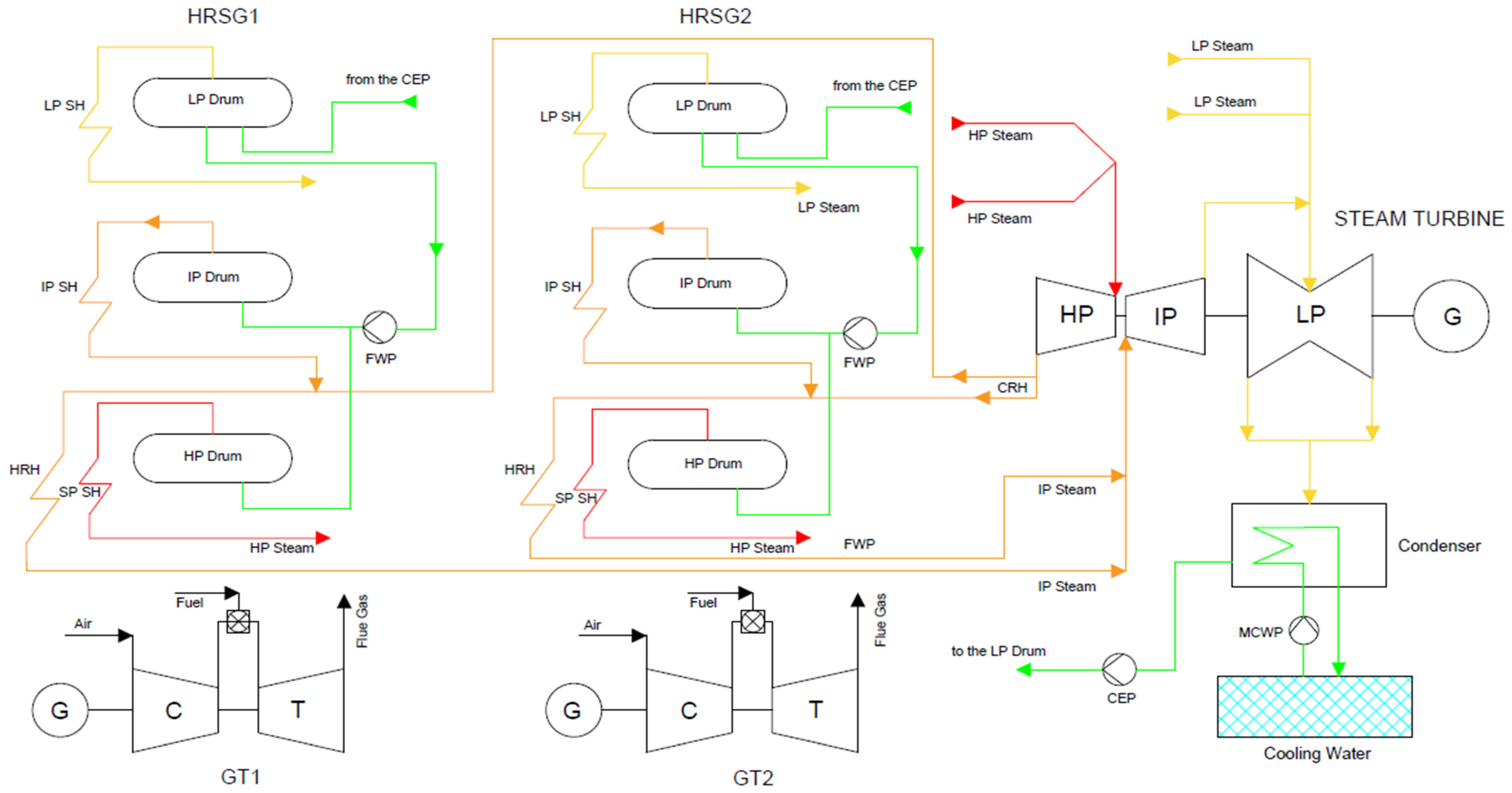
Figure 1. The CCPP flow diagram.
Energies 18 05110 g001
Figure 2. The CCPP data flow diagram.
Energies 18 05110 g002
Figure 3. ANN structure.
Energies 18 05110 g003
Figure 4. Outlier plot of parameters.
Energies 18 05110 g004
Figure 5. Correlation matrix.
Energies 18 05110 g005
Figure 6. Regression model performances without seasonal segmentation.
Energies 18 05110 g006
Figure 7. Regression model performances for AT < 12 °C.
Energies 18 05110 g007
Figure 8. Regression model performances for 12 °C ≤ AT < 20 °C.
Energies 18 05110 g008
Figure 9. Regression model performances for AT ≥ 20 °C.
Energies 18 05110 g009
Figure 10. Shapley plots for the global Rational Quadratic GPR model and the three temperature-segmented models.
Energies 18 05110 g010
Figure 11. Scatter plot of actual and predicted values of EPO.
Energies 18 05110 g011
Figure 12. Residual distributions for different AT segments.
Energies 18 05110 g012
Figure 13. Scatter plots of actual and predicted EPO based on ANN.
Energies 18 05110 g013
Figure 14. Rolling-Window Giacomini–White test plot.
Energies 18 05110 g014
Figure 15. Comparison of Model Predictions for AT < 12 °C.
Energies 18 05110 g015
Table 1. Statistical characteristics of the dataset.
MinMaxMeanStd. Deviation
EPO860.30950.56901.5427.46
AT4.1630.6218.146.13
RH24.61100.0074.6111.91
V0.0220.0590.0390.006
AP982.541027.781010.205.13
Table 2. Bootstrap-based prediction results.
Bootstrap (B = 2000)Confidenceq_low (residual)q_high (residual)Average Width (MW)Empirical CoverageMean Winkler ScoreMean Interval Score
95%−6.39255.342211.73470.949715.743715.7437
Disclaimer/Publisher’s Note: The statements, opinions and data contained in all publications are solely those of the individual author(s) and contributor(s) and not of MDPI and/or the editor(s). MDPI and/or the editor(s) disclaim responsibility for any injury to people or property resulting from any ideas, methods, instructions or products referred to in the content.