Article

A High-Precision, All-Rectangle-Based Method Linearly Concave Hydropower Output in Long-Term Reservoir Operation

by
Hao Zheng
1,2,3,
Yan Huang
1,4,
Yongqiang Wang
1,2,
Feixiang Hou
5,
Yong Xu
5,
Cheng Chen
3,5,
Suzhen Feng
3,6 and
Jinwen Wang
3,7,*
1
Water Resources Management, Changjiang River Scientific Research Institute, Wuhan 430010, China
2
Hubei Key Laboratory of Water Resources & Eco-Environmental Sciences, Changjiang River Scientific Research Institute, Wuhan 430010, China
3
Hubei Key Laboratory of Digital River Basin Science and Technology, Huazhong University of Science and Technology, Wuhan 430074, China
4
College of Hydraulic & Environmental Engineering, China Three Gorges University, Yichang 443002, China
5
Faculty of Electric Power Engineering, Kunming University of Science and Technology, Kunming 650500, China
6
College of Automation and Electronic Engineering, Qingdao University of Science and Technology, 99 Songling Road, Qingdao 266061, China
7
School of Civil and Hydraulic Engineering, Huazhong University of Science and Technology, Wuhan 430074, China
*
Author to whom correspondence should be addressed.
Energies 2025, 18(19), 5102; https://doi.org/10.3390/en18195102
Submission received: 28 August 2025 / Revised: 22 September 2025 / Accepted: 23 September 2025 / Published: 25 September 2025

Abstract

The nonlinearity and non-convexity of the hydropower output function (HOF) make it very challenging to search for the optimal solution to the hydropower scheduling problem, which, however, can be more easily solved with consistency by mathematical programming if the HOF can be properly linearized with high accuracy. In this paper, a detailed review of different linear concaving approximation methods to model the HOF is presented, and a high-precision, all-rectangle linear concaving approximation method is proposed. It avoids the drawback of existing rectangular grid linear approximation methods which introduce a large number of integer variables and reduce solution efficiency by avoiding the accurate expression of fitting error at the corner points. It is mathematically proved that the method based on this rectangular subdivision can converge to any concave function with arbitrary precision as the grid resolution increases. The approximated results of the output functions of the four cascaded hydropower plants in the Lancang River show that both the proposed method and the existing method can reduce the average fitting error from 2.16% of installed capacity to 1.49% compared to the high-efficiency method. Although the proposed method is slower in solving speed than the high-efficiency method, it is significantly better than the unstable existing method.

1. Introduction

As a widely recognized renewable resource, the development and utilization of hydropower is an effective pathway to reducing carbon emissions and mitigating the adverse impacts of global climate change. Beyond substantial installed capacity, hydropower offers crucial operational flexibility, therefore it is indispensable in modern power systems with high penetrations of variable renewable energy. Long-term hydropower scheduling (LTHS) seeks to determine generation strategies over multi-year or annual horizons to maximize system-wide benefits [1]. In practice, the objective function typically combines firm power and total energy production, both of which are vital for supply reliability and sustainable use of water resources. Because LTHS provides key insights into the expected value of stored water, it has long been an internationally prominent topic in the energy–water nexus. Concurrently, recent engineering studies show that setting end-of-dry-season drawdown targets and performing rolling multi-year simulations can have a material impact on annual generation and firm output, further underscoring hydropower’s central role in low-carbon portfolios [2]. In practical long–medium–short operations, the accuracy of head-dependent modeling at the long-term layer is pivotal, which in turn motivates high-quality linearization of the hydropower production function over the storage–discharge domain [3,4].
Nevertheless, LTHS is inherently a large-scale, discrete, nonlinear, and non-concave optimization problem. The complexity is particularly pronounced in the coordinated long-horizon operation of cascaded systems, where release processes and inter-reservoir interactions must be jointly managed. This challenge is further compounded by the nonlinear and non-concave hydropower output function (HOF), which couples generating discharge and hydraulic head—the latter being jointly determined by storage and outflow. Accurately capturing the hydro–energy relationships while maintaining computational tractability remains a central challenge in this field [5]. For long-term horizons, head variation is substantial, making the HOF strongly head-dependent [6].
To address these challenges, a wide range of optimization techniques have been proposed in the literature, including nonlinear programming (NLP) [7,8,9], dynamic programming (DP) [10,11], linear programming (LP) [12,13,14], and intelligent or metaheuristic algorithms (MA) [15]. Marcelino et al. [16] use a heuristic optimization method in Brazil to improve hydropower generation with lower water use. Evolutionary algorithms are widely used for handling nonlinear, nonconcave problems. Nonlinear models are capable of representing the physical system with high fidelity and are thus often considered a natural choice for hydropower scheduling. However, the global optimum cannot generally be guaranteed because the concavity of the formulated problem is uncertain when nonlinear hydropower output limitations are considered. DP is widely used for its ability to handle nonlinear, non-smooth objectives and constraints via stage-wise optimization, but it is susceptible to the “curse of dimensionality” in large cascades [17], mixed integer linear programming (MILP) formulations remain a widely used approach in mathematical programming [18], provided that the HOF is linearized with sufficient care. The feasibility and accuracy of the resulting schedules are strongly influenced by the specific strategy adopted for partitioning and interpolating the bivariate surface.
Metaheuristic algorithms have become increasingly popular in recent decades due to their flexibility in handling nonlinearities and complex constraints [15]. Genetic algorithms, particle swarm optimization, and simulated annealing have been successfully applied in multi-reservoir systems [19]. Recent advances integrate these approaches with mathematical programming to improve efficiency and stability, such as hybrid DP-PSO methods or GA-SA approaches for reservoir scheduling. For example, Baima et al. [20] proposed a GA-based hybrid procedure that reduces spillage through “push–pull” strategies, thereby improving scheduling efficiency and stability. However, these methods are often inconsistent in producing near-optimal solutions within reasonable computational time and may face difficulties when feasible regions are irregular.
LP and its variants have long been applied to hydropower system optimization due to their solid theoretical foundations and scalability. LP-based approaches can solve large-scale decision problems efficiently and guarantee global optima. Since LTHS is fundamentally nonlinear, it is usually necessary to linearize the problem to leverage the computational advantages of LP. The nonlinearity and non-concavity of LTHS are primarily attributable to the HOF, which is a function of generating discharge and reservoir head, the latter being dependent on both storage and outflow. Thus, the success of applying LP methods critically depends on the quality of HOF linearization. Pérez-Díaz et al. [21] compared plant-based and unit-based production functions. Their study shows that the plant-based model can better capture the head losses in common waterways and generally achieves higher revenues in most scenarios, though it requires preprocessing to construct an aggregate function and cannot fully represent unit-level differences. In contrast, the unit-based model accurately describes unit start-ups and operating constraints and is suitable for independent waterway configurations, but it may overestimate output when ignoring coupling effects, leading to lower overall revenues than the plant-based model.
Numerous methods have been proposed for modeling and linearizing the HOF. The simplest linear treatment assumes hydropower output is proportional to turbine discharge, with a constant head and water consumption rate across the scheduling horizon [22]. While convenient, this approach is highly imprecise and unsuitable for systems where head variation significantly affects generation [23]. Piecewise linearization provides a more accurate global approximation and can be solved using MILP. Thus, any tractable linearization should approximate a genuinely bivariate surface rather than a single-variable curve. To this end, several linearization strategies that explicitly incorporate the head effect have been explored, such as representing HOF in terms of head and storage [24], generating discharge and storage [25], average storage [26], or storage and total outflow including spillage [4,27], head and generating discharge [28,29]. Both rectangular and triangular grids have been adopted for piecewise approximation. Kang [30] proposed an efficient one-dimensional linearization method for short-term hydro-thermal scheduling, in which reservoir storage is discretized and the power–discharge curves under fixed storage levels are piecewise linearized. This approach effectively avoids large-scale coupled integer variables while accurately representing the hydropower HOF in the model. Conejo [31] approximated the aggregated HOF in intra-plant hydro economic operation using three output curves under different net heads and formulated an incremental model with linear functions and binary variables to search for the optimal solution. Borghetti et al. proposed a general representation in which each hydropower station’s HOF is expressed as a curve consisting of a fixed number of linear segments. To find the optimal solution for every unit’s curve throughout the scheduling horizon, the method introduces a decomposed convex-combination formulation between the power-output points of these linear segments [32]. Guisández et al. [33] compared five linear programming formulations of the hydro production function, proposed the binary function method, and found that the logarithmic branching method is the most accurate for daily stages, while the binary function method is more effective for weekly stages. Methodological analyses further show that when the net head axis is segmented first and each slice is linearized in discharge, the resulting rectangular partition balances accuracy with implement ability, and careful elimination of redundant binaries/constraints improves efficiency without sacrificing feasibility. Empirical evidence from self-scheduling studies indicates that head-layering is the chief computational bottleneck; hence, rectangular meshing—paired with compact Special Ordered Sets of type II (SOS2) formulations—materially reduces solve time while maintaining fidelity to the original head–discharge surface [31]. Recent advances go further by reconstructing SOS2 via binary branching under rectangular meshing, achieving logarithmic scaling of binary variables and demonstrating strong accuracy–efficiency trade-offs on multi-reservoir Chinese cascades. Finally, from a modeling perspective, rectangular meshes align naturally with SOS2, the classic ordered-set device for piecewise linear interpolation, and therefore provide a clean algebraic interface to modern MILP solvers [34].
In recent years, research has increasingly sought to improve piecewise linearization methods to achieve high accuracy without introducing integer variables. Concave hull (CH) techniques have been employed to approximate nonlinear HOF [35,36,37,38,39]. The CH of a set of points represents the smallest concave set containing them, which generally results in overestimation of functional values since nonlinear functions are enclosed from the outside. Gomes e Souza et al. [40] proposed a partitioning strategy for the hydro production function (HPF), using convex hull approximations in concave regions, multiple-choice linearization in convex regions, and iterative head updates to balance accuracy and computational efficiency. In the Aggregated Convex Combination approach, Special Ordered Sets of type 2 are introduced into the integer-programming formulation to select the triangular or rectangular grid cell in which the Aggregated Convex Combination will take place [41]. The LOG method [42] is characterized by requiring a number of binary variables that is logarithmic (base-2) in the number of the intervals of flow and net head considered, plus at the most six. It operates with a non-orthogonal mesh made up of triangles, which allows it to account for both head-power and head-flow limit dependencies, assigning an active plane to approximate the HOF within or near each grid. This concaving approach avoids consistent overestimation and reduces fitting errors. Triangular grid-based linear concaving (TTBLC) models [39] are efficient in CPU time but often suffer from low accuracy, particularly in low-capacity reservoirs where precise head effects significantly influence results. On the other hand, rectangular grid concaving models (e.g., PWL1 [12]) can provide results comparable to SOS2 linearization but encounter difficulties since adjacent active planes may overlap, failing to share common edges and introducing inconsistencies. These observations, together with evidence from MILP-based scheduling under rectangular meshing, therefore, motivate the pursuit of rectangle-centric linear concaving schemes that preserve the computational benefits of structured partitions while mitigating classical corner and overlap issues. Moreover, market-based and operational studies indicate that, if meshing is poorly structured, head discretization often dominates computing time, reinforcing the need for efficient rectangular partitions.
The existing TTBLC method offers some efficiency in CPU time but suffers from low accuracy, especially in small-capacity reservoirs where head effects are critical. This is because triangular grids often lead to large fitting errors in low-storage regions, failing to capture head dependence precisely. Moreover, triangular meshing introduces rigid corner constraints and discontinuous partitions, which cause overestimation and inconsistencies. As a result, TTBLC cannot simultaneously ensure high precision and numerical stability, limiting its practical effectiveness. In contrast, the PWL1 method based on rectangular grid points can achieve lower fitting errors and perform better in fitting the actual power output of hydropower stations under the same grid resolution. However, when PWL1 is used to calibrate the parameters of the convex hull plane that approximates HOF, the Special Ordered Sets of type I (SOS1) is introduced. When using the solver to interpret SOS1, integer variables are introduced, which further increases the difficulty of solving the calibration model. Under finite time and high grid resolution, the optimal solution of the calibration model cannot be obtained, thereby limiting the acquisition of more accurate convex hull plane parameters. Therefore, it is necessary to develop a method, similar to the PWL1 approach, that can precisely fit the HOF without introducing integer variables, while also having a convergent form and competitive running time.
Against this backdrop, this paper proposes an all-rectangle-grid global linear concaving (ARBLC) method that performs high-precision linearization of the nonlinear HOF without introducing any integer variables. The method partitions the storage–discharge domain into rectangular grids and uses a global comparison mechanism to ensure that each active plane is valid at least at its grid center. Compared with PWL1, ARBLC avoids rigid corner-error constraints, thereby preserving model flexibility and improving computational efficiency. It can be shown that, as grid resolution increases, ARBLC approximates any concave function to arbitrary accuracy, providing a firm theoretical basis for its high-precision characteristics. Numerical experiments indicate that ARBLC significantly reduces computational burden while maintaining approximation accuracy, effectively alleviating the long-standing precision–efficiency trade-off in hydropower scheduling.
The remainder of this paper is structured as follows. Section 2 first outlines the nonlinear and non-concave characteristics of long-term reservoir scheduling and then introduces several linear concaving models for the hydropower output function, including the SOS1-based piecewise linearization (PWL1), the efficient triangular-grid linearization (TTBLC) and the all-rectangle grid concaving model (ARBLC). Section 3 presents the mathematical proof for the high-precision rectangular-grid method, showing that as the grid resolution increases the method can approximate concave (or concave) functions with arbitrarily small error approaching zero in the limit and discusses the limitations of triangular gridding schemes. Section 4 evaluates the fitting accuracy and computational efficiency of these linearization methods using benchmark test functions and case studies from actual hydropower plants. Section 5 summarizes the main findings and outlines directions for future research.

2. Problem Formulation

2.1. Nonlinearity in Hydropower Scheduling Problem

The LTHS is a fortnightly hydropower generation optimization problem that aims to maximize firm power and annual energy production while accounting for the end-of-horizon storage constraint [12]. In essence, it is a nonlinear programming model determined by the nonlinear characteristics of the HOF. The average reservoir storage and release serve as the two primary decision variables, jointly determining the water level, power output, water consumption rate, and ultimately the HOF, which can be expressed as: the average reservoir storage and the release serve as the two primary decision variables that collectively determine the water level, power output, water consumption rate, and ultimately the HOF itself, expressed as
P r t = f r ( Q r t , V ¯ r t ) ,
where r and t are subscript indices of reservoirs and time-steps, respectively; P r t is the power output of reservoir r in t in MW; Q r t is the release from reservoir r in t in m3/s; V ¯ r t is the average water volume of r in t .
Fortunately, it can be simplified by linearizing the nonlinear functions and reformulating the LTHS problem.

2.2. Linear Concaving Models

In our previous research [39], we found that hydropower output increases with higher reservoir releases. However, once the release exceeds the specified generation capacity, further increases no longer enhance energy production and may even reduce output due to the rise in tailwater level, which decreases the effective head. Therefore, the hydropower output, defined by (1), can be approximately regarded as a concave function to be maximized in the LTHS problem. A linearized concave modeling approach is employed, which approximates the hydropower output function using a series of cutting planes, as illustrated in Figure 1 The defining plane is expressed as
f ^ n ( V , Q ) = a n Q + b n V + c n ,
and the HOF can be approximated by the following functions:
P r t a r n Q r t + b r n V ¯ r t + c r n = f ^ r n ( Q r t , V ¯ r t ) ( n = 0 , , N 1 ) ,
where a , b , c are parameters to be determined for the plane; n and N are the index and number of the planes, respectively.
Equation (3) ensures that the lowest boundary among all planes is used to approximate the HOF. By maximizing the objective function of the LTHS problem, the optimal solution is driven toward the boundary or minimum of these planes. This transformation converts the original nonlinear problem into a linear programming formulation without introducing any integer variables. To estimate the parameters of these planes, an optimization model must be constructed based on the original output values calculated from the HOF [39]; this model is essentially a quadratic programming problem. Since the output function of each hydropower plant is estimated independently, indices for hydropower plants and time steps are omitted from the mathematical expressions in this section.

2.2.1. Gridding and Definition

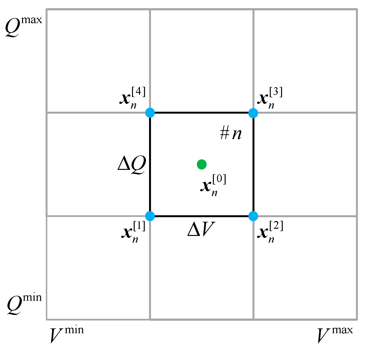
The domain of the HOF is discretized into rectangular grids, as illustrated in Figure 2. Both storage and release are uniformly partitioned into NV and NQ intervals, respectively, spanning their corresponding lower and upper bounds. The storage segment interval ΔV and the release segment interval ΔQ can be calculated by the following formulas:
Δ V = V max V min N V ,
Δ Q = Q max Q min N Q ,
where V r min and Q r min are the minimum storages and the minimum release of r, respectively; V r t max is the maximum storages of r at the beginning of t; Q r t max is the maximum release from reservoir r in t.
The feasible region is discretized into N = N V × N Q rectangular grids, which are sequentially indexed as follows:
n = u ( i , j ) = i * N Q + j ( n = 0 , 1 , N 1 ) .
In Equation (6), each rectangular grid n corresponds one-to-one with the combination (i, j):
i = i ( n ) j = j ( n ) .
As illustrated in Figure 2, the storage and release are discretized into NV + 1 values and NQ + 1 values, respectively. The coordinates of these discrete points can therefore be calculated as follows:
V ( i ) = V min + i Δ V ( i = 0 , 1 , 2 , N V ) ,
Q ( j ) = Q min + j Δ Q ( j = 0 , 1 , 2 , N Q ) .
A point is defined as
X = V Q .
As illustrated in Figure 2, the coordinates of a point are defined as
X i j = V ( i ) Q ( j ) ,
and each grid (n) will be represented by four grid points for fitting error assessment, along with a center point denoted as follows:
X n [ m ] = ( V n [ m ] , Q n [ m ] ) T ( m = 0 , 1 , 2 , 3 , 4 ) ,
and which are denoted as
X n [ 0 ] = [ V ( i + 0.5 ) , Q ( j + 0.5 ) ] T X n [ 1 ] = [ V ( i ) , Q ( j ) ] T X n [ 2 ] = [ V ( i + 1 ) , Q ( j ) ] T X n [ 3 ] = [ V ( i + 1 ) , Q ( j + 1 ) ] T X n [ 4 ] = [ V ( i ) , Q ( j + 1 ) ] T ,
where X n [ 0 ] is the center point of the rectangular grid n and others are the corner points of the rectangular grid.
For the convenience of the following description, the plane Equation (12) can be expressed as
f ^ n ( X ) = A n X + c n A n = [ a n , b n ] .

2.2.2. Piecewise Linearization with SOS1 (PWL1)

Kang [12] presented a piecewise linearization method (PWL1) that divides the variable domain into rectangular grids; each grid has an active plane to approximate the HOF in or near it. For a specific hydroplant, following the same discretization logic, its output function is discretized into values shown in the table of Figure 2.
The parameters in the (2) that define planes are estimated by solving the following model:
Objective:
min i = 0 N V j = 0 N Q [ f ( X i j ) f ^ ( X i j ) ] 2 ,
subject to
f ^ n X n [ 0 ] f ^ k X n [ 0 ] ( k n ; n , k = 0 , 1 , 2 , , N 1 ) ,
f ^ X i j = min f ^ n 1 X i j , n 1 = u ( i , j ) f ^ n 2 X i j , n 2 = u ( i 1 , j ) f ^ n 3 X i j , n 3 = u ( i , j 1 ) f ^ n 4 X i j , n 4 = u ( i 1 , j 1 ) .
The linearization of the “min” constraint can be formulated using SOS1 [12]. It should be noted that if a point lies on the boundary of the domain, some of the adjacent planes ( n 1 , n 2 , n 3 , n 4 ) are not present in Equation (17).

2.2.3. Three-Triangle-Based Linear Concaving (TTBLC)

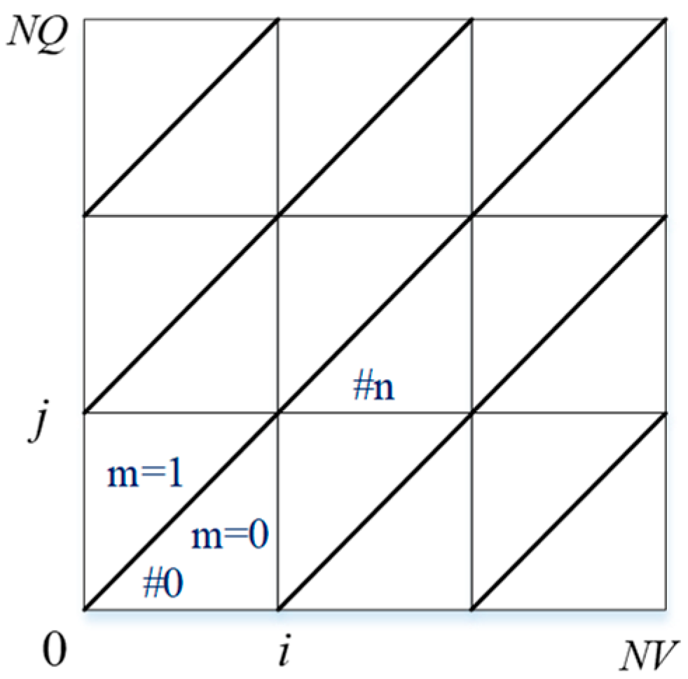
The objective of calibrating the plane parameters is to minimize the sum of squared fitting errors between the estimated and actual power outputs at all three corner points and one center point within each triangular grid region defined by Equation (2) over the feasible domain in Figure 3. This can be mathematically expressed as
min n = 0 N α ( e r r n [ 0 ] + e r r n + [ 0 ] ) 2 + β m = 1 3 ( e r r n [ m ] + e r r n + [ m ] ) 2 ,
subject to
f ^ n ( X n [ m ] ) e r r n [ m ] + e r r n + [ m ] = f ( X n [ m ] ) ( n = 0 , 1 , , N 1 ; m = 0 , 1 , 2 , 3 ) ,
f ^ n ( X n [ 0 ] ) f ^ k ( X n [ 0 ] ) ,   ( k Φ ( n ) ; n = 0 , 1 , , N 1 ) ,
f ^ l ( X i j ) = f ^ k ( X i j ) ( k , l Θ ( i , j ) ; k l ; i ( j ) = 0 , 1 , , N V ( N Q ) ) ,
e r r n [ m ] , e r r n + [ m ] 0 ( n = 0 , 1 , , N 1 ; m = 0 , 1 , 2 , 3 ) .
Here, the number of triangles N is
N = 2 × N V × N Q .
Here, the e r r n [ m ] and e r r n + [ m ] are the negative and positive fitting errors from X n [ m ] ; α and β are the weights of middle and corner points, respectively. Φ ( n ) is the set of triangular grids that are edge-adjacent to triangular grid n ; Θ ( i , j ) is the set of triangular grids that share a cross point X i j . In this work, for α = 3 and β = 1 , the weight ( α ) is assigned to 3 so as to balance the weight of the center point with that of the three corners of a triangular grid.

2.2.4. All Rectangle Based Linear Concaving (ARBLC)

The PWL1 method employs integer variables during the modeling of active plane parameters, with point values defined according to Equation (17). This approach considerably increases computational complexity and solution time. In contrast, our earlier work on All Triangle-Based Linear Concaving (ATBLC) [39] demonstrated that omitting integer variables can significantly enhance the solution efficiency of linear concaving models. However, the triangle-based method suffers from certain limitations that reduce its accuracy in approximating hydropower output—a issue that will be discussed in detail later. To overcome these drawbacks, the proposed method in this study retains the rectangular subdivision scheme of PWL1, while incorporating the grid point valuation concept from the triangle-based approach. Specifically, the value at each grid point is determined based on its corresponding intersecting plane.
In the PWL1 method, the rectangular-partition-based concave hull plane model introduces SOS1. When the solver interprets SOS1, it requires integer variables, which increases the computational complexity of fitting the HOF. To avoid introducing integer variables, the method refrains from precisely representing the fitting error at the corner points. Instead, the objective function of the model is constructed by evaluating each grid corner point.
The objective of plane parameter calibration is to minimize the sum of squared errors between the fitted and actual power outputs at all four corner points of each rectangular grid within the feasible region, The specific mathematical formulation of the model is as follows:
F n min = min A , c n = 1 N ( Δ Ω ) k = 1 4 f ( X n [ k ] ) f ^ n ( X n [ k ] ) 2 ,
where f ( X n [ k ] ) represents the actual power output value at the corner point X n [ k ]
Subject to
f ^ n ( X n [ 0 ] ) f ^ k ( X n [ 0 ] ) ( k n ; n , k = 0 , 1 , 2 N 1 ) ,
where the f ^ n ( X ) is defined in Equation (14).

2.2.5. Summary of Three Models

Table 1 summarizes the variable and constraint counts of each linear concaving model developed for HOF approximation. The discretization resolution is uniformly defined by the parameter N, where NV = NQ = N represent the numbers of intervals for storage and release, respectively. Notably, PWL1 is the only model that introduces binary variables—a subclass of integer variables. Under identical discretization resolution, TTBLC and ARBLC maintain an equal ratio between variable count and number of approximation planes, meaning both models require identical variable quantities for a fixed number of planes. Moreover, ARBLC employs fewer constraints than PWL1 at the same resolution, which further contributes to its computational efficiency. For N > 4, TTBLC achieves the smallest number of constraints among all evaluated models.

3. Convergence Proof

This section will theoretically and numerically demonstrate that the ARBLC method achieves zero-convergent fitting error for concave functions, while also examining the limitations of the triangle-based approach.

3.1. Mathematical Proof

Error definition:
f ^ ( X ) = min n f ^ n ( X ) ,
E r r = Ω f ( X ) f ^ ( X ) 2 d Ω ,
where d Ω represents the area of each grid subregion after uniformly partitioning the feasible domain Ω into N grids, which can also be denoted as Δ Ω . When N ( Δ Ω ) , Δ Ω = 0 . Here, f ^ ( X ) is the approximate value of point x calculated using the linear concaving method.
Lemma 1 
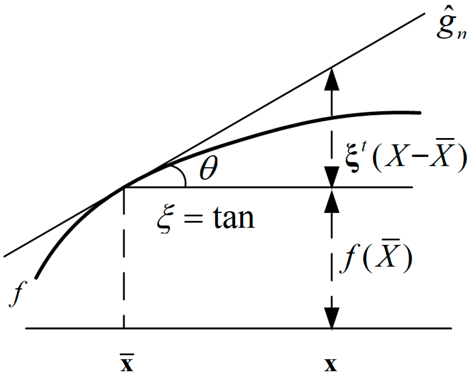
([43]). Let  Ω  be a nonempty concave set in  R n n, and let  f : Ω R  be concave. Then for any  X ¯ Ω , there exists a vector  ξ  such that
f ( X ) f ( X ¯ ) + ξ T ( X X ¯ )     for   X Ω ,
where  ξ  is a subgradient of  f  at  X ¯ .
Proof. 
By Lemma (28), for a concave function f there exists a set of planes g ^ L in the feasible domain in Figure 4 defined as
g ^ i ( X ) = f ( X i [ 0 ] ) + ξ i T ( X X i [ 0 ] ) ,
g ^ ( X ) = min i   g ^ i ( X ) ,
where l is the plane number, L is the total number of planes, and ξ l T is the subgradient of the concave function f at X i [ 0 ] as well as the normal vector to the plane l.
From (29),
g ^ j ( X i [ 0 ] ) = f ( X j [ 0 ] ) + ξ j T ( X i [ 0 ] X j [ 0 ] ) ( 29 ) f ( X i [ 0 ] ) = ( 30 ) g ^ i ( X i [ 0 ] ) .
Obviously, g ^ L ( X ) is a feasible solution to the problem with objective (24) subject to (25). Thus, the objective value at the optimum must be less than or equal to that at any feasible solution,
F n min = i = 1 n ( Δ Ω ) k = 1 4 f ( X i [ k ] ) f ^ i * ( X i [ k ] ) 2 G n = i = 1 n ( Δ Ω ) k = 1 4 f ( X i [ k ] ) g ^ i ( X i [ k ] ) 2 ,
where f ^ i * ( X ) is the optimum. Then,
lim n F n min Δ Ω 4 = lim Δ Ω 0 i = 1 n ( Δ Ω ) 1 4 k = 1 4 f ( X i [ k ] ) f ^ i * ( X i [ k ] ) 2 Δ Ω = lim Δ Ω 0 i = 1 n ( Δ Ω ) f ( X i [ 0 ] ) f ^ i * ( X i [ 0 ] ) 2 Δ Ω = ( 25 ) lim Δ Ω 0 i = 1 n ( Δ Ω ) f ( X i [ 0 ] ) f ^ * ( X i [ 0 ] ) 2 Δ Ω = Ω [ f ( X ) f ^ * ( X ) ] 2 d Ω = E r r * 0 ,
which represents the fitting error in linearly concaving the original concave function [f(X)] by the optimal hyperplanes [ f ^ i * ( X ) ] ,
f ^ * ( X ) = min n   f ^ n * ( X ) .
On the other hand,
lim n G n Δ Ω 4 = lim Δ Ω 0 i = 1 n ( Δ Ω ) 1 4 k = 1 4 f ( X i [ k ] ) g ^ i ( X i [ k ] ) 2 Δ Ω = lim Δ Ω 0 i = 1 n ( Δ Ω ) f ( X i [ 0 ] ) g ^ i ( X i [ 0 ] ) 2 Δ Ω = ( 31 ) 0 ,
which, based on (32) and (33), suggests
E r r * = 0 ,
which indicates the approximating error will infinitely approach zero by increasing the gridding resolution. This is made possible by the feasible hyperplanes [ g ^ i ( X ) ] that ensure each grid has a point [ X i [ 0 ] ] where the fitting error is zero. □

3.2. The Missing Part in TTBLC

In our previous work [39], we proposed a TTBLC method, which discretizes the storage and release domain uniformly into triangular grids. Within each grid, a local active plane is used to approximate the nonlinear function. Since two adjacent active planes share a common edge along the interface of their corresponding triangular grids, local concavity guarantees global concavity. This property significantly reduces computational effort, resulting in markedly faster Central Processing Unit (CPU) times.
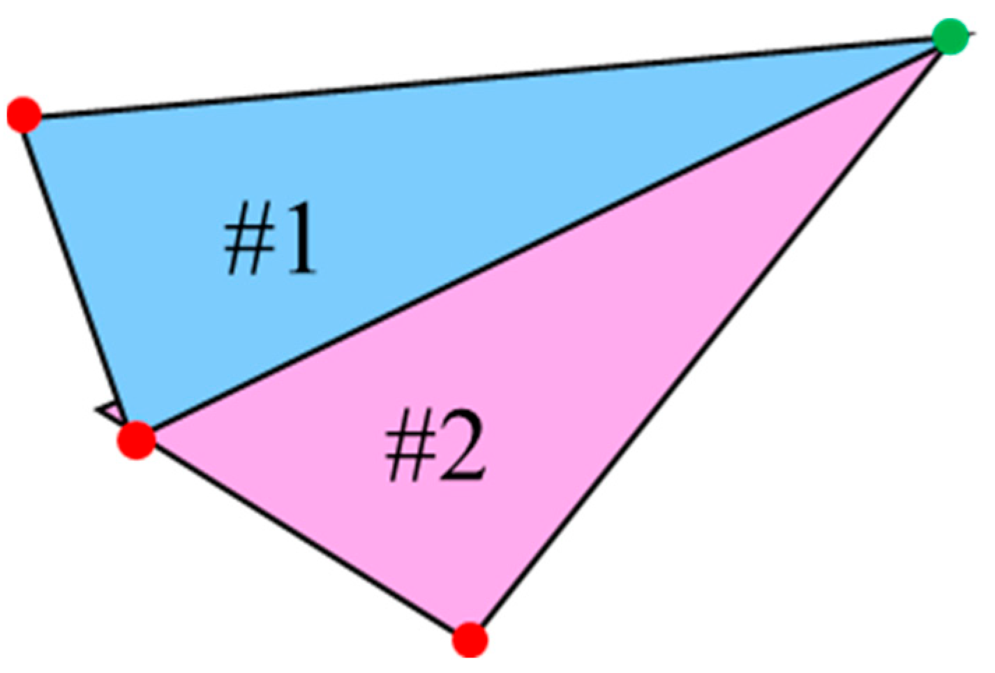
Unfortunately, the TTBLC method may not achieve asymptotically zero fitting error through increased gridding resolution, as it currently cannot reliably identify feasible active planes that ensure at least one point per grid exhibits zero fitting error. A natural alternative is to constrain adjacent active planes to intersect at the original nonlinear function’s surface vertices, thereby enforcing zero fitting error at all corners of each triangular grid. However, the feasibility of such a configuration cannot be guaranteed. A counterexample is illustrated in Figure 5, where the surface formed by two adjacent active planes in triangular grids (#1 and #2) fails to remain concave. This occurs specifically when the functional value at the green grid point is significantly lower than those at the red grid points.
However, it may be possible to develop a gridding strategy that ensures both global concavity through local concavity preservation and the feasibility of active planes such that each grid contains at least one point with zero fitting error. Research on this approach is currently ongoing.

3.3. Numerical Tests

3.3.1. Testing Function

The fitting performance of the three linear concaving models will be tested by using
f ( x , y ) = 200 ( x 10 ) 2 ( y 10 ) 2 ,
which is strictly a concave function of variables x and y, and the functional value is nonnegative when x , y [ 0.10 ] . Here, this work uses the f ( x i , y j ) as a hydropower output function by converting the points X i j into values in range [0, 10] with
x i = V ( i ) V min V max V max × 10 y j = Q ( i ) Q min Q max Q max × 10 ,
and then
f ( x i , y j ) = f ( X i j ) .

3.3.2. Error Assessment

In this paper, the accuracy of the linear approximation will be evaluated based on the root-mean-square error (RMSE), maximum absolute error (MAE), relative error (RE) and mean relative error (MRE). Each performance measure is expressed as
R M S E = k = 1 K f ^ * ( X k ) f ( X k ) 2 K ,
M A E = max k f ^ * ( X k ) f ( X k ) ,
R E = f ^ * ( X k ) f ( X k ) f ( X k ) × 100 % ,
M R E = 1 K k = 1 K f ^ * ( X k ) f ( X k ) f ( X k ) ,
where X k is the k-th sample point; f ^ * ( X k ) determined by Equation (34) is the calculated value by the optimal hyperplanes at the Xk; K is the number of sample points to be evaluated, which set to be 101 × 101 = 10,201 in all the cases of this work.
The Gurobi 9.0.2 solver is employed to solve the three linear concaving models, which are formulated as quadratic programming problems. All computations are carried out under the default solver settings, without additional prescaling or manual adjustments to the barrier/simplex tolerances or stopping criteria. For the barrier tolerance, the default value of BarConvTol is 1 × 10⁻⁸. The default value of MarkowitzTol, which is related to the simplex tolerance, is 0.0078125, and the default value of OptimalityTol is 1 × 10⁻⁶. As for the stopping criteria, besides the tolerance—based stopping conditions, the default value of BarIterLimit for the barrier method is 1000.
The models are implemented in C++, which is also used to perform the optimal piecewise linear fitting of the given point sets. The computations are executed on a personal computer equipped with an AMD Ryzen 7 4800H processor (2.90 GHz) and 16 GB of RAM. To enhance reproducibility, the test functions and station-fitting scripts can be provided upon request.

3.3.3. Three Models for Testing Function

Table 2 summarizes the main performance metrics for the approximation of the test function across various grid resolutions. For each combination of resolution and model, the table provides the RMSE (in MW), MAE (in MW), and the central processing unit (CPU) time (in seconds). Cases where Gurobi reported an “out of memory” error are marked with an “X”. The minimum and maximum RMSE values in each row are highlighted in green and red, respectively.
As indicated in Table 2, the approximation error of all three methods decreases as the number of planes increases. Owing to its triangular discretization scheme, TTBLC utilizes half the number of release segments compared to the rectangular-based methods under an equivalent total number of planes. For instance, a configuration of 256 planes in TTBLC corresponds to a resolution of N V × N Q = 16 × 8 . At the same number of planes, the RMSE of the proposed ARBLC method remains within 7.27% of that achieved by the benchmark PWL1 method, whereas the high-efficiency TTBLC exhibits a considerably larger deviation of at least 27.35%. Under these conditions, ARBLC demonstrates a minimal deviation of merely 1.76%. Although computationally slower than TTBLC, ARBLC delivers significantly faster solution times than PWL1. When the number of planes reaches or exceeds 324, the PWL1 model triggers an “out of memory” error during solution attempts. This failure stems primarily from its incorporation of integer variables, which necessitate a branch-and-bound algorithm within the Gurobi solver—a process that exhausts available memory before identifying a feasible solution for this quadratic programming problem. Furthermore, across all tested plane counts, ARBLC consistently yields the lowest MAE, suggesting a more uniform distribution of fitting errors compared to PWL1.
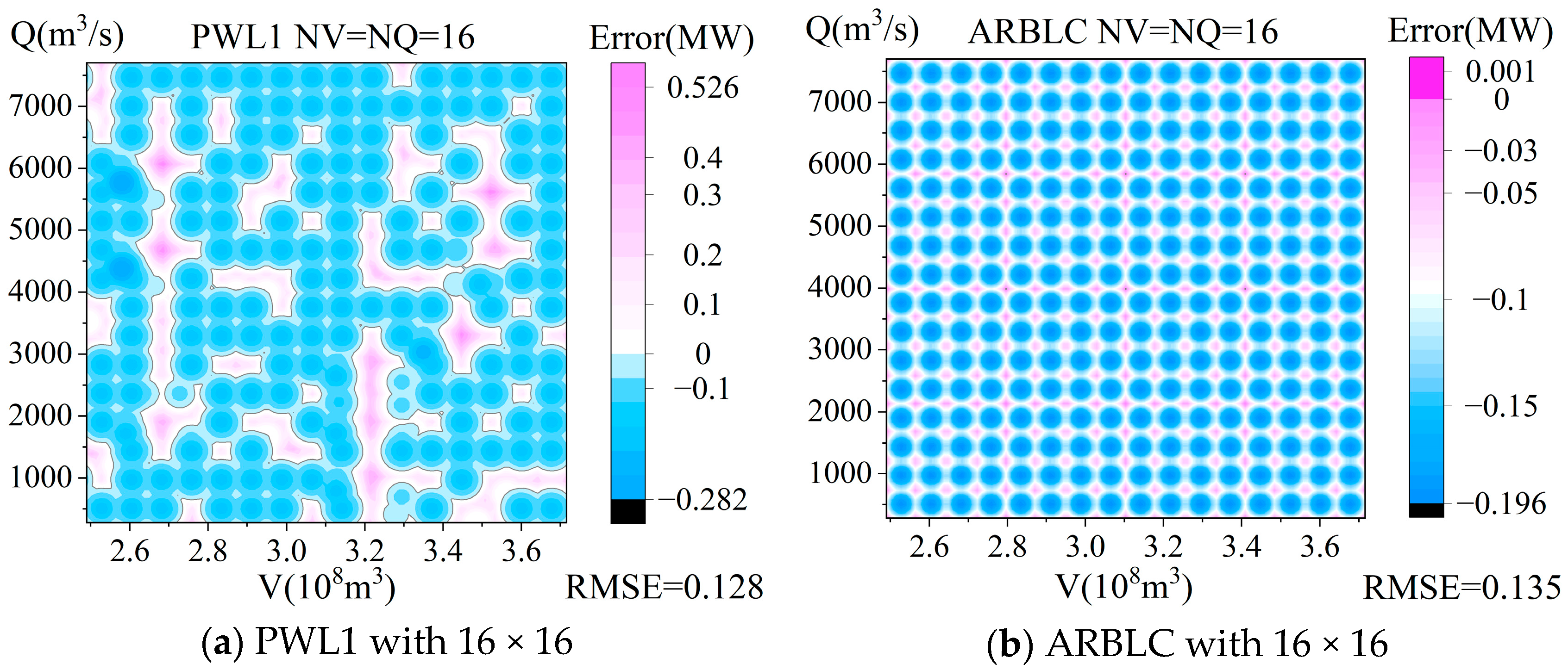
ARBLC achieves a superior fitting effect with significantly less computational time compared to PWL1. For example, ARBLC attains an RMSE of 0.107 MW in only 66.28 s, whereas PWL1 requires 856.76 s to reach a higher RMSE of 0.128 MW. Furthermore, ARBLC consistently yields the minimum ME in each comparison row, indicating a more uniform distribution of fitting errors.
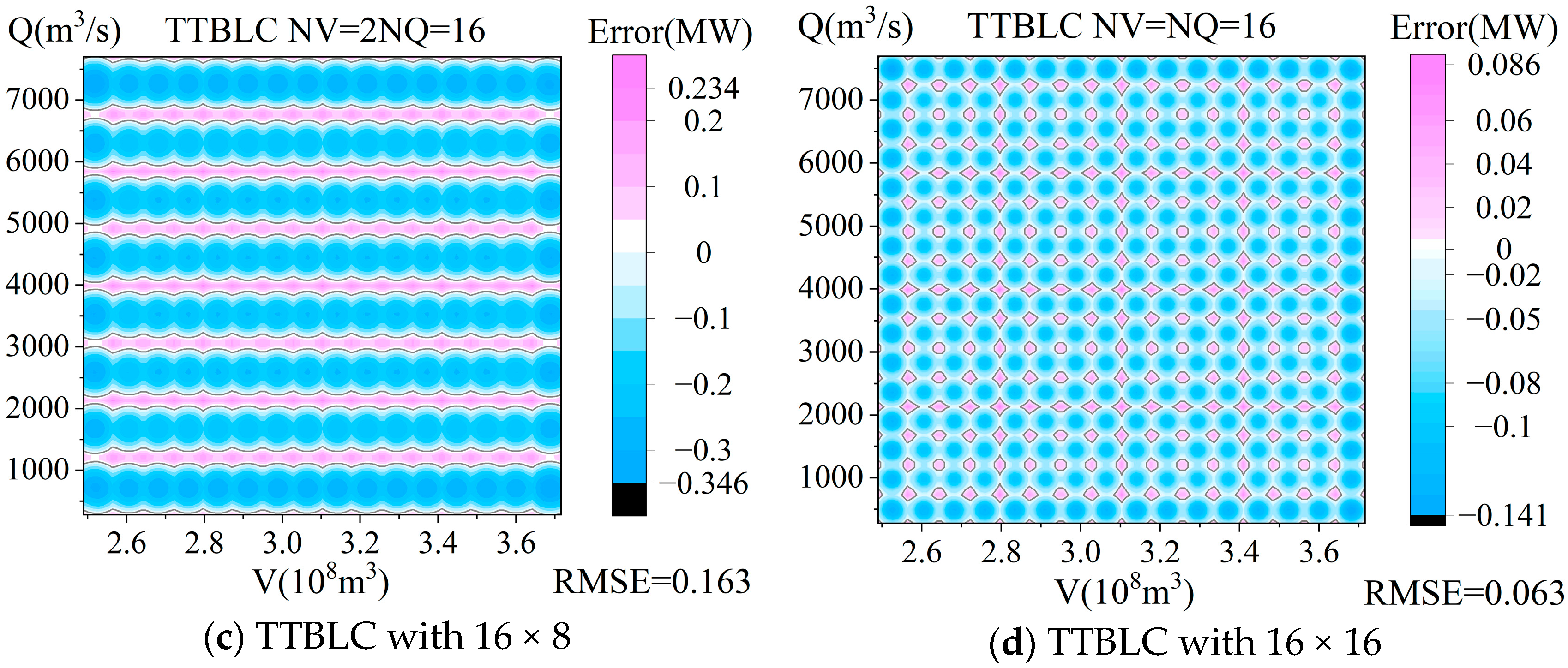
To facilitate a comparative analysis of the performance of the three models in fitting the test function, the error distributions are illustrated in Figure 6. Here, the error is defined as the deviation between the model-fitted values and the original output values, with the black line representing the zero-error contour. As can be observed, the errors of the three linear concaving models are uniformly distributed across rectangular grid cells when approximating the test function. Within each grid cell, the error exhibits a radial pattern: the deviation decreases from positive values at the corners to negative values toward the center, a behavior inherently influenced by the characteristics of the test function itself.
Figure 6a–c illustrate that the three models are applied to 256 grids, while Figure 6d shows that TTBLC is applied to 512 grids. Figure 6a demonstrates that the distribution of fitting errors for PWL1 is insufficiently uniform, with error values in some grids being entirely positive. From Figure 6b, both the maximum and minimum errors of ARBLC are smaller than those of PWL1. Furthermore, the fitting errors of ARBLC for the test function are non-positive across all regions, with errors at individual sample points being zero only in isolated cases. In other words, the concave surface fitted by ARBLC lies entirely below the test function surface. As the gridding resolution increases, the generated surface fits the concave test function surface more closely in an upward trend, and errors within individual grids decrease accordingly. From Figure 6c,d, it can be observed that the surface optimized by TTBLC differs significantly from that of ARBLC; this is primarily because the error values at the corners of each grid cell are all positive.

3.3.4. Convergence of ARBLC for Testing Function

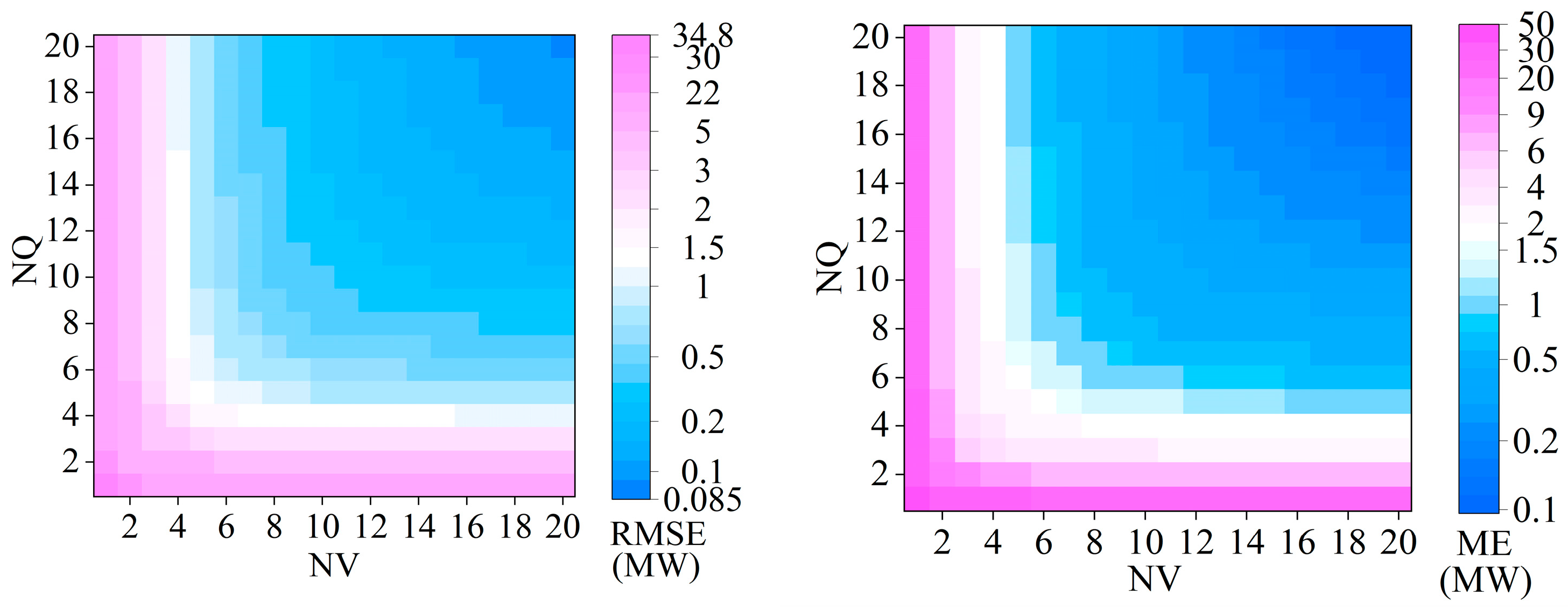
Figure 7 shows the RMSE and ME of the ARBLC fitting testing function with different gridding resolutions. It can be seen from Figure 7 that the changing trends of RMSE and MAE are consistent. When the value of NV(NQ) is the same, as the value of another discrete number NQ(NV) increases, the RMSE and ME by ARBLC decrease accordingly, that is, as the number of grids increases, the fitting accuracy of ARBLC is correspondingly improved. It is worth noting that when the number of planes is the same, the smaller the difference between NV and NQ, the better the fitting effect, which is mainly determined by the axisymmetric characteristics of the testing function. According to Figure 7, when the feasible region is divided into infinite grids, the RMSE of the testing concave function fitted by ARBLC can converge to zero.

4. Numerical Examples

4.1. Engineering Background

The models are applied to four hydropower reservoirs in the Lancang River, in the southwest of China. The Lancang River cascade is a typical large-scale hydropower reservoir system that consists of large hydropower reservoirs with different operability levels. Table 3 gives some of the basic characteristics of these hydropower reservoirs.

4.2. Concavity Based on Original Data

In our previous research [39], we obtained the HOFs for Xiaowan, Manwan, Dachaoshan, and Nuozhadu. These functions were derived by linearly interpolating the original data within the lower and upper bounds given in Table 3. The HOFs of all four hydroplants are monotonically increasing functions of storage, generally exhibiting a concave shape but with local irregularities in the regions constrained by generating capacity. These irregularities occur because the generating capacity is disabled over certain ranges of water heads, which is more pronounced in the Manwan and Dachaoshan hydroplants.

4.3. Comparison Between the Three Models

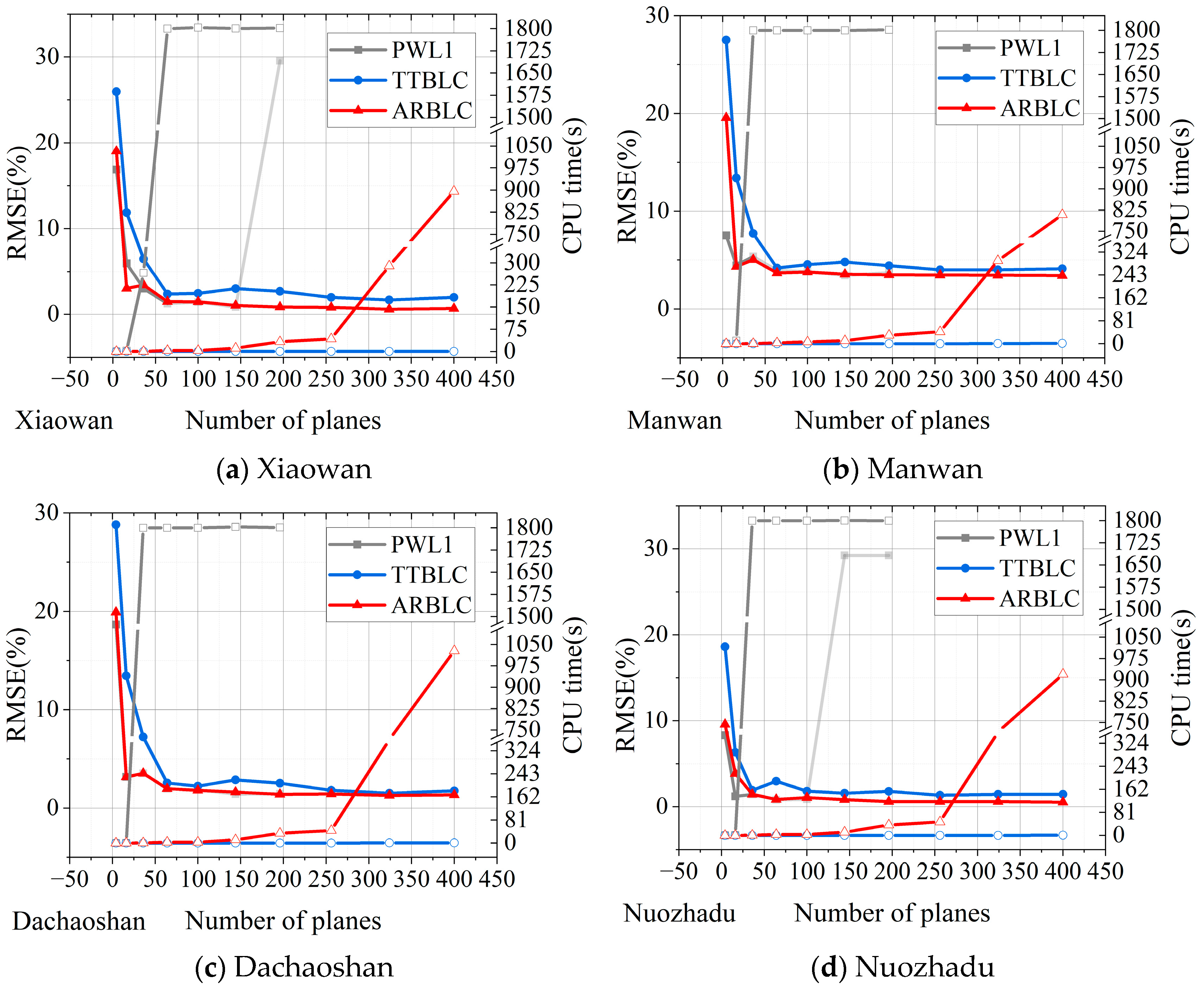
Figure 8 compares the three models (TTBLC, ARBLC, and PWL1) in terms of CPU time and RMSE for the linear concave approximation of HOFs across the four hydroplants in the Lancang River. The upper limit for CPU time in fitting the HOFs of these hydroplants is set to 1800 s. If the fitting time reaches this limit without yielding an optimal solution, the corresponding RMSE value is displayed in a lighter color in the figure. As shown in Figure 8, when the grid count is the same and exceeds 25, the RMSE values of ARBLC and PWL1 are nearly identical, indicating their equivalence in approximating nonlinear HOFs. Moreover, the results show that ARBLC outperforms TTBLC in fitting accuracy. Specifically, when the grid count exceeds 324, the average RMSE for HOF fitting across Xiaowan, Manwan, Dachaoshan, and Nuozhadu using ARBLC is 1.49%, compared to 2.16% for TTBLC. For these four hydroplants, the RMSE values from ARBLC are 0.61%, 3.46%, 1.30%, and 0.58%, respectively, whereas TTBLC yields 1.69%, 4.01%, 1.52%, and 1.43%. ARBLC shows faster convergence of RMSE compared to TTBLC at lower grid counts. Figure 8 also highlights ARBLC’s advantage over PWL1 in computational stability, which becomes increasingly significant as the number of grids exceeds 36, and becomes highly pronounced for grid counts greater than 144. Notably, when the grid count exceeds 196, PWL1 fails to provide acceptable results for Xiaowan and Nuozhadu. When the grid count does not exceed 144, both ARBLC and TTBLC require less than 12 s of CPU time, which is acceptable for practical purposes. For instance, when using 100 grids, ARBLC takes 3.34 s to fit the HOF for Xiaowan with an RMSE of 1.48% of the installed capacity, which represents a 65% improvement in accuracy over TTBLC, which has an RMSE of 2.44% with a fitting time of 0.12 s. This demonstrates that ARBLC has a clear advantage over TTBLC when higher fitting accuracy is required within a relatively flexible time constraint for approximating nonlinear HOFs.
In conclusion, for fitting the actual HOFs, among the three linear concaving model the existing method PWL1 achieves the highest accuracy, followed by the ARBLC method proposed in this chapter, while the high-efficiency TTBLC method demonstrates the lowest precision. In terms of computational time and stability, TTBLC requires the shortest time, followed by ARBLC, while PWL1 requires the longest time and exhibits unstable performance. When computational time is less critical but higher fitting accuracy is prioritized, the ARBLC method is recommended.

4.4. Distribution of Fitting Errors

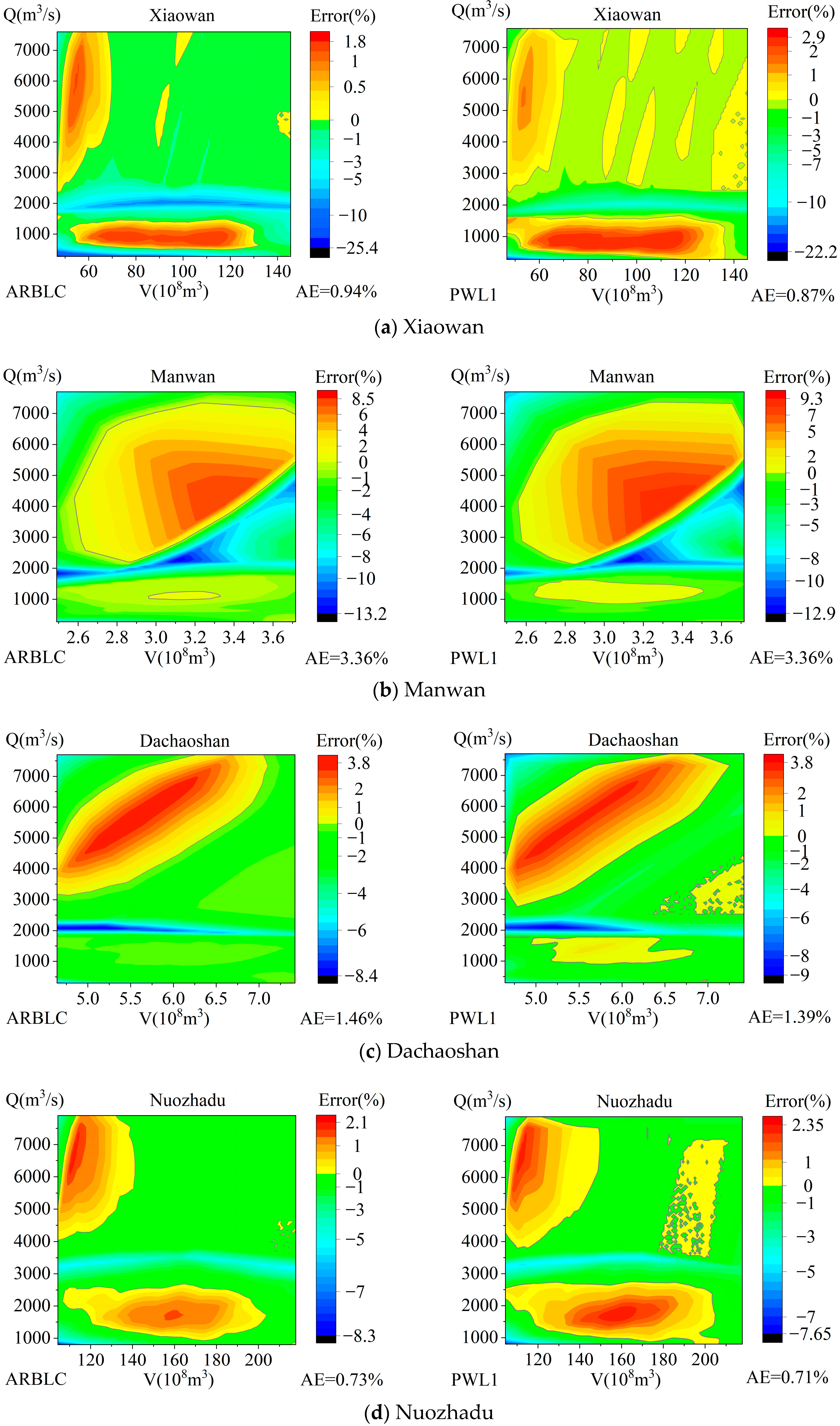
Figure 9 compares the RE distributions obtained by applying ARBLC and PWL1 to four hydroplants using a grid resolution of 100 (10 × 10 grids). In the figure, RE and ARE are determined by Equations (42) and (43), respectively. The black line represents the contour with an RE value of zero. It can be seen that the RE distributions of the two models are very similar when fitting the HOFs of the same hydroplant. Both models result in RE distributions that are split into upper and lower parts, with fitting errors generally tending to be negative. The largest negative errors typically occur near the division line area, which is the intersection of the output surface determined by the outflow and the output surface determined by the generation capacity. The approximation in this area tends to yield larger errors. From Figure 9a,d, it can be observed that Xiaowan and Nuozhadu, which have better operability, exhibit a similar pattern in RE distribution, with the largest positive errors occurring in an ‘L’ shape. In contrast, Figure 9b,c show that Manwan and Dachaoshan, with lower operability, have a similar RE distribution pattern, where the largest positive errors occur in a ‘Q’ shape. Overall, the proposed ARBLC method shows performance comparable to the existing PWL1 method in approximating the actual HOFs of hydropower plants.

4.5. Convergence of ARBLC for Hydroplants

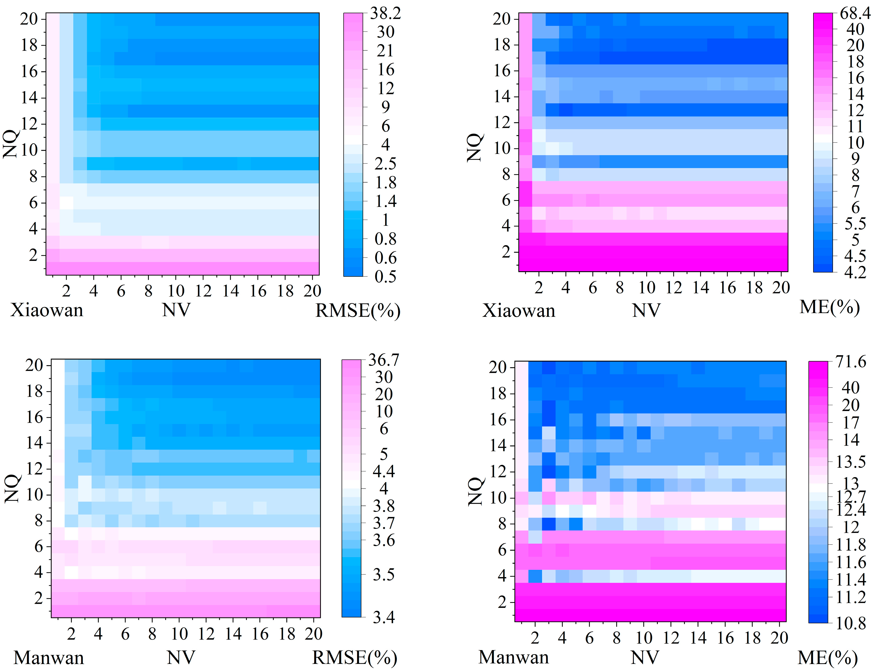
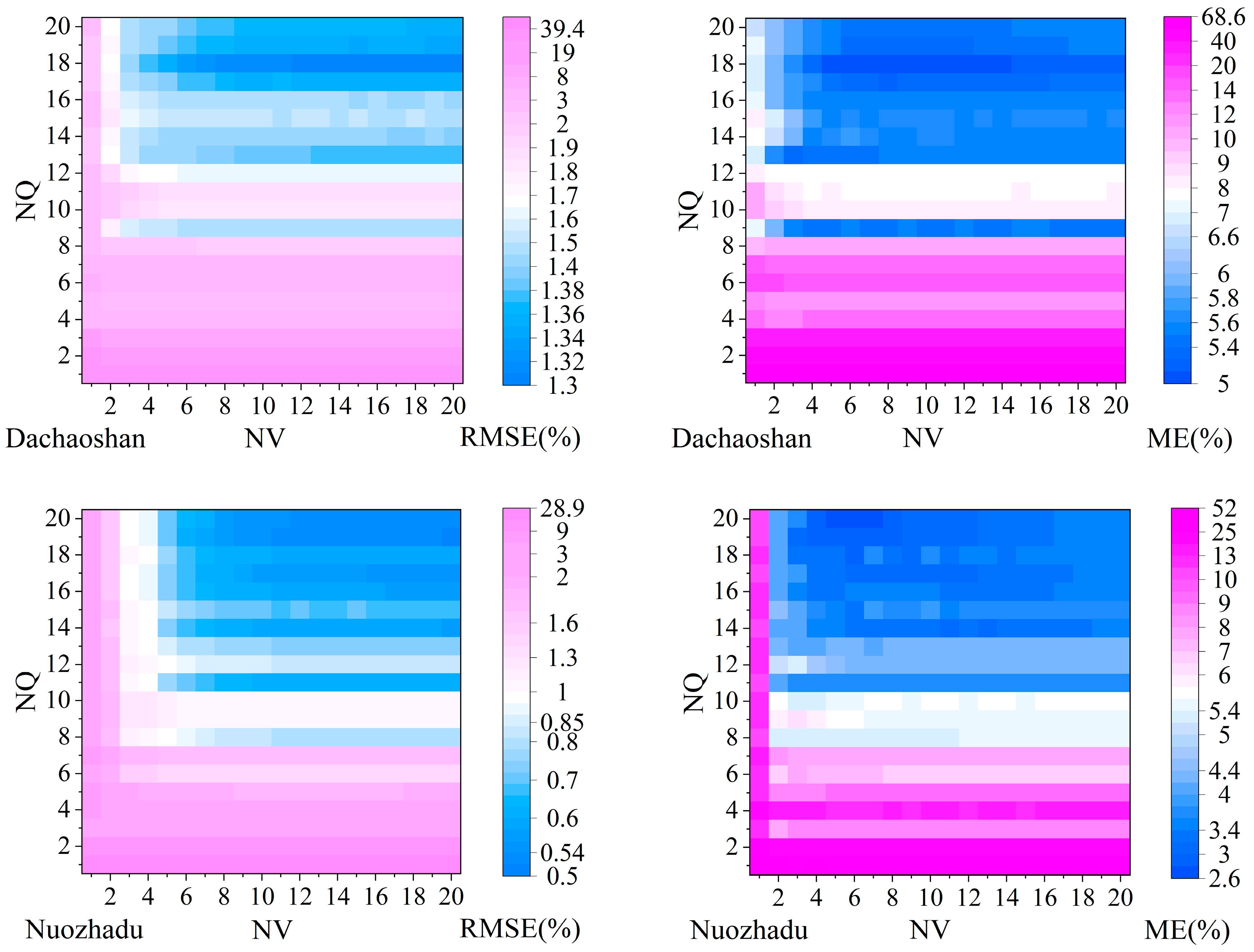
Figure 10 presents the RMSE and MAE, expressed as percentages of the installed capacity, for four hydropower plants using the ARBLC method under different grid resolutions. As shown, the distributions of RMSE and MAE exhibit similar trends across various discretization configurations. The discrete number for outflow, NQ, is identified as the dominant factor influencing both error metrics. When NQ is less than 8, regardless of the NV value, both RMSE and MAE are significantly higher than those observed at resolutions where NQ > 12 and NV > 4. Notably, holding either NV or NQ constant while increasing the other does not result in a monotonic decrease in RMSE or MAE. For instance, results from the Xiaowan plant demonstrate that ARBLC achieves RMSE values of 0.89%, 0.64%, and 0.97% at resolutions of 12 × 9, 12 × 13, and 12 × 15, respectively. These outperform the corresponding values of 1.47%, 0.86%, and 0.83% obtained at resolutions of 12 × 10, 12 × 14, and 12 × 16. This non-monotonic behavior is attributed to the physical characteristics of hydropower output, as further illustrated in Figure 8 and Figure 9. Actual power output is constrained by the maximum installed capacity. When the reservoir release exceeds the maximum discharge for power generation, output saturates at the maximum level, a region where the ARBLC approximation exhibits increased deviation. A higher discretization number NQ enables finer segmentation along the outflow dimension, improving the method’s ability to capture nonlinearities in this region and thereby reducing fitting error.
In summary, higher grid resolution does not systematically improve the accuracy of ARBLC in approximating real-world HOF and may incur unnecessary computational cost. These findings highlight the importance of selectively choosing discretization parameters rather than universally pursuing higher resolution.

5. Conclusions

This paper proposes a global rectangular grid-based linear concaving approximation method (ARBLC), which provides an effective solution for the high-precision linearization of HOFs. By employing rectangular subdivision of the feasible region of hydropower output, the four corner points of each rectangular grid are used to evaluate the errors in the objective function. This method avoids the precise representation of fitting errors at the corner points, eliminating the need for integer variables and enabling more efficient and reliable calibration of the high-precision concave hull plane parameters for approximating HOFs. The existence of a feasible set of hyperplane solutions ensures that within each rectangular grid, there is at least one point where the fitting error is zero. This mathematically proves that the rectangular subdivision-based approximation method can converge to any concave function with arbitrary precision as the grid resolution increases, while highlighting the limitations of existing triangulation-based methods. The proposed ARBLC method is compared with the existing rectangular grid-based linear approximation method (PWL1) and the high-efficiency linear approximation method (TTBLC) from our previous work, applied to approximate the HOF of four hydropower stations in the Lancang River cascade. The following conclusions are drawn from the numerical results:
Approximation of test functions: The ARBLC method exhibits fitting performance that is closer to the PWL1 method and significantly outperforms the high-efficiency TTBLC method in terms of approximation accuracy. With the same number of planes, the relative increase in RMSE for ARBLC compared to PWL1 does not exceed 7.27%, whereas TTBLC shows a relative increase of no less than 27.35%. The relative increase for ARBLC is only 1.76%. Furthermore, the error distribution of all three piecewise linear approximation methods for the test concave function is structured based on rectangular grid cells. Compared to PWL1, ARBLC shows a more uniform error distribution.
Approximation of real hydropower output functions: The test results for the four hydropower stations in the Lancang River cascade show that both ARBLC and PWL1 reduce the average fitting error from 2.16% of the installed capacity to 1.49%, compared to the high-efficiency TTBLC method. Although ARBLC is slower than TTBLC, it significantly outperforms the unstable PWL1 method. When higher accuracy is required for approximating the actual HOF of hydropower stations, and computational time is not critical, the ARBLC method is highly recommended.
Grid resolution and fitting performance: When using ARBLC to approximate the real hydropower station HOF, higher grid resolution does not always result in better fitting performance. Blindly choosing higher grid resolutions may lead to a waste of computational resources. It is recommended to balance the discretization numbers of reservoir volume (NV) and outflow (NQ) within the same grid resolution. In certain cases, setting NQ > NV can improve fitting results.
In conclusion, the ARBLC method proposed in this paper is a high-precision linear concaving approximation method for linearly approximating nonlinear HOFs. Based on rectangular subdivision of the feasible region, it ensures high-precision approximation of the HOF using calibrated concave hull planes, helping to accurately describe the nonlinear characteristics of the original problem and maximize the utilization of hydropower resources. This method holds strong application potential in solving practical hydropower optimization scheduling problems, especially in cases where computational time is not critical, but high solution accuracy is required. While ARBLC improves solution reliability by avoiding the introduction of integer variables and improves upon existing rectangular grid methods, there is still room for further enhancement in solving efficiency. Therefore, it is necessary to further analyze the efficiency of TTBLC and explore ways to further improve the computational efficiency of the ARBLC method while maintaining its fitting accuracy.

Supplementary Materials

The following supporting information can be downloaded at: https://www.mdpi.com/article/10.3390/en18195102/s1.

Author Contributions

Conceptualization, H.Z. and J.W.; software, C.C.; data curation, H.Z. and Y.W.; writing—original draft preparation, H.Z., S.F. and C.C.; writing—review and editing, Y.H., Y.W. and J.W.; visualization, F.H., Y.X. All authors have read and agreed to the published version of the manuscript.

Funding

This research was funded by the National Natural Science Foundation Key Project of China grant number U2340211, the Fundamental Research Funds for Central Public Welfare Research Institutes grant number CKSF20231036/SZ and CKSF20241021/SZ, the National Natural Science Foundation Key Project of Hubei grant number 2022CFD027 and 2024AFA011, the Major Scientific and Technological Projects of the Ministry of Water Resources grant number SKS-2022120, Projects of China Yangtze Power Co., Ltd. grant number Z242302057, And the APC was funded by the Fundamental Research Funds for Central Public Welfare Research Institutes grant number CKSF20241021/SZ.

Data Availability Statement

The data are contained within the article and Supplementary Materials.

Acknowledgments

Special thanks are given to the anonymous reviewers and editors for their constructive comments.

Conflicts of Interest

The authors declare no conflict of interest.

References

  1. Chen, C.; Feng, S.; Liu, S.; Zheng, H.; Zhang, H.; Wang, J. A stochastic linear programming model for maximizing generation and firm output at a reliability in long-term hydropower reservoir operation. J. Hydrol. 2023, 618, 129185. [Google Scholar] [CrossRef]
  2. Liu, S.; Luo, X.; Zheng, H.; Zhang, C.; Wang, Y.; Chen, K.; Wang, J. Investigation on Water Levels for Cascaded Hydropower Reservoirs to Drawdown at the End of Dry Seasons. Water 2023, 15, 362. [Google Scholar] [CrossRef]
  3. Zhao, Z.; Cheng, C.; Yan, L. An efficient and accurate Mixed-integer linear programming model for long-term operations of large-scale hydropower systems. IET Renew. Power Gener. 2021, 15, 1178–1190. [Google Scholar] [CrossRef]
  4. Guisández, I.; Pérez-Díaz, J.I. Mixed integer linear programming formulations for the hydro production function in a unit-based short-term scheduling problem. Int. J. Electr. Power Energy Syst. 2021, 128, 106747. [Google Scholar] [CrossRef]
  5. Feng, S.; Zheng, H.; Qiao, Y.; Yang, Z.; Wang, J.; Liu, S. Weekly hydropower scheduling of cascaded reservoirs with hourly power and capacity balances. Appl. Energy 2022, 311, 118620. [Google Scholar] [CrossRef]
  6. Candela-Ripoll, I.; Otaola-Arca, P.; García-González, J.; Rivero-Honegger, C.; Mariño-Lizuain, F. Optimal discretization of net head dependency in heterogeneous multi-reservoir hydroelectric systems. In Proceedings of the 2021 IEEE Madrid PowerTech 2021, Madrid, Spain, 28 June–2 July 2021; IEEE: New York, NY, USA, 2021. [Google Scholar]
  7. Li, C.; Zhou, J.; Ouyang, S.; Ding, X.; Chen, L. Improved decomposition–coordination and discrete differential dynamic programming for optimization of large-scale hydropower system. Energy Conv. Manag. 2014, 84, 363–373. [Google Scholar] [CrossRef]
  8. Azevedo, A.T.; Oliveira, A.R.L.; Soares, S. Interior point method for long-term generation scheduling of large-scale hydrothermal systems. Ann. Oper. Res. 2008, 169, 55–80. [Google Scholar] [CrossRef]
  9. Catalao, J.P.S.; Mariano, S.J.P.S.; Mendes, V.M.F.; Ferreira, L.A.F.M. Scheduling of Head-Sensitive Cascaded Hydro Systems: A Nonlinear Approach. IEEE Trans. Power Syst. 2009, 24, 337–346. [Google Scholar] [CrossRef]
  10. Löhndorf, N.; Wozabal, D.; Minner, S. Optimizing Trading Decisions for Hydro Storage Systems Using Approximate Dual Dynamic Programming. Oper. Res. 2013, 61, 810–823. [Google Scholar] [CrossRef]
  11. He, Z.; Wang, C.; Wang, Y.; Wei, B.; Zhou, J.; Zhang, H.; Qin, H. Dynamic programming with successive approximation and relaxation strategy for long-term joint power generation scheduling of large-scale hydropower station group. Energy 2021, 222, 119960. [Google Scholar] [CrossRef]
  12. Kang, C.; Chen, C.; Wang, J. An Efficient Linearization Method for Long-Term Operation of Cascaded Hydropower Reservoirs. Water Resour. Manag. 2018, 32, 3391–3404. [Google Scholar] [CrossRef]
  13. Feng, Z.-K.; Niu, W.-J.; Wang, S.; Cheng, C.-T.; Jiang, Z.-Q.; Qin, H.; Liu, Y. Developing a successive linear programming model for head-sensitive hydropower system operation considering power shortage aspect. Energy 2018, 155, 252–261. [Google Scholar] [CrossRef]
  14. Ilich, N. Shortcomings of linear programming in optimizing river basin allocation. Water Resour. Res. 2008, 44, W02426. [Google Scholar] [CrossRef]
  15. Sörensen, K. Metaheuristics—The metaphor exposed. Int. Trans. Oper. Res. 2015, 22, 3–18. [Google Scholar] [CrossRef]
  16. Marcelino, C.G.; Camacho-Gómez, C.; Jiménez-Fernández, S.; Salcedo-Sanz, S. Optimal Generation Scheduling in Hydro-Power Plants with the Coral Reefs Optimization Algorithm. Energies 2021, 14, 2443. [Google Scholar] [CrossRef]
  17. Wang, C.; Zhou, J.; Lu, P.; Yuan, L. Long-term scheduling of large cascade hydropower stations in Jinsha River, China. Energy Conv. Manag. 2015, 90, 476–487. [Google Scholar] [CrossRef]
  18. Peng, W.; Jiang, Z.; Xu, Y.; Zhao, Z.; Zhu, F.; Gao, J.; Lu, P. Medium to long-term optimization model for cascade hydropower plants under high penetration of variable renewable energy. Renew. Energy 2025, 254, 123739. [Google Scholar] [CrossRef]
  19. Zhang, J.; Guo, A.; Wang, Y.; Chang, J.; Wang, X.; Wang, Z.; Tian, Y.; Jing, Z.; Peng, Z. How to achieve optimal photovoltaic plant capacity in hydro-photovoltaic complementary systems: Fully coupling long-term and short-term operational modes of cascade hydropower plants. Energy 2024, 313, 134161. [Google Scholar] [CrossRef]
  20. Baima, D.; Qian, G.; Luo, J.; Wang, P.; Zheng, H.; Wang, J. Monthly hydropower scheduling of cascaded reservoirs using a genetic algorithm with a simulation procedure. Energies 2024, 17, 3756. [Google Scholar] [CrossRef]
  21. Pérez-Díaz, J.I.; González-Martínez, J. Comparison between plant-based and unit-based production functions for the day-ahead energy and reserve scheduling of a hydropower plant with common waterways. Energy Syst. 2023. [Google Scholar] [CrossRef]
  22. Dubost, L.; Gonzalez, R.; Lemaréchal, C. A Primal-Proximal Heuristic Applied to the Unit-Commitment Problem; INRIA: Le Chesnay, France, 2003. [Google Scholar]
  23. Harou, J.J.; Pulido-Velazquez, M.; Rosenberg, D.E.; Medellín-Azuara, J.; Lund, J.R.; Howitt, R.E. Hydro-economic models: Concepts, design, applications, and future prospects. J. Hydrol. 2009, 375, 627–643. [Google Scholar] [CrossRef]
  24. Hjelmeland, M.N.; Zou, J.; Helseth, A.; Ahmed, S. Nonconvex Medium-Term Hydropower Scheduling by Stochastic Dual Dynamic Integer Programming. IEEE Trans. Sustain. Energy 2019, 10, 481–490. [Google Scholar] [CrossRef]
  25. Hamann, A.; Hug, G.; Rosinski, S. Real-Time Optimization of the Mid-Columbia Hydropower System. IEEE Trans. Power Syst. 2017, 32, 157–165. [Google Scholar] [CrossRef]
  26. Rodriguez, J.A.; Anjos, M.F.; Cote, P.; Desaulniers, G. MILP Formulations for Generator Maintenance Scheduling in Hydropower Systems. IEEE Trans. Power Syst. 2018, 33, 6171–6180. [Google Scholar] [CrossRef]
  27. Goor, Q.; Kelman, R.; Tilmant, A. Optimal-multipurposemultireservoir-operation-model-with-variable-productivity-of-hydropower-plants. Water Resour. Plann Manag. 2011, 137, 258–267. [Google Scholar] [CrossRef]
  28. Lin, M.; Shen, J.; Cheng, C.; Lü, Q.; Wang, Y. Long-term multi-objective optimal scheduling for large cascaded hydro-wind-photovoltaic complementary systems considering short-term peak-shaving demands. Energy Convers. Manag. 2024, 301, 118063. [Google Scholar] [CrossRef]
  29. dos Santos Abreu, D.L.; Finardi, E.C. Continuous Piecewise Linear Approximation of Plant-Based Hydro Production Function for Generation Scheduling Problems. Energies 2022, 15, 1699. [Google Scholar] [CrossRef]
  30. Kang, C.; Wu, S.; Gul, E.; Yu, X.; Ren, P. A 1D linearization–based MILP–NLP method for short-term hydrothermal operation. Int. J. Low-Carbon Technol. 2022, 17, 540–549. [Google Scholar] [CrossRef]
  31. Conejo, A.J.; Arroyo, J.M.; Contreras, J.; Villamor, F.A. Self-scheduling of a hydro producer in a pool-based electricity market. IEEE Trans. Power Syst. 2002, 17, 1265–1272. [Google Scholar] [CrossRef]
  32. Borghetti, A.; D’Ambrosio, C.; Lodi, A.; Martello, S. An MILP approach for short-term hydro scheduling and unit commitment with head-dependent reservoir. IEEE Trans. Power Syst. 2008, 23, 1115–1124. [Google Scholar] [CrossRef]
  33. Guisández, I.; Périz-Diáz, J.I. Linear Programming Formulations for the Hydro Production Function in a Water Value Calculation. Renew. Energy 2025, 243, 122571. [Google Scholar] [CrossRef]
  34. Beale, E.M.L. Branch and bound methods for numerical optimization of non-convex functions. Comput. Stat. 1980, 80, 11–20. [Google Scholar]
  35. Belloni, A.; Lima, A.D.; Maceira, M.P.; Sagastizábal, C.A. Bundle Relaxation and Primal Recovery in Unit Commitment Problems. The Brazilian Case. Ann. Oper. Res. 2003, 120, 21–44. [Google Scholar] [CrossRef]
  36. Santos, K.V.; Finardi, E.C. Piecewise linear approximations for hydropower production function applied on the hydrothermal unit commitment problem. Int. J. Electr. Power Energy Syst. 2022, 135, 107464. [Google Scholar] [CrossRef]
  37. Diniz, A.L.; Maceira, M.E.P. A Four-Dimensional Model of Hydro Generation for the Short-Term Hydrothermal Dispatch Problem Considering Head and Spillage Effects. IEEE Trans. Power Syst. 2008, 23, 1298–1308. [Google Scholar] [CrossRef]
  38. Fredo, G.L.M.; Finardi, E.C.; de Matos, V.L. Assessing solution quality and computational performance in the long-term generation scheduling problem considering different hydro production function approaches. Renew. Energy 2019, 131, 45–54. [Google Scholar] [CrossRef]
  39. Zheng, H.; Feng, S.; Chen, C.; Wang, J. A new three-triangle based method to linearly concave hydropower output in long-term reservoir operation. Energy 2022, 250, 123784. [Google Scholar] [CrossRef]
  40. e Souza, H.G.; Finardi, E.C.; Brito, B.H.; Takigawa, F.Y.K. Partitioning approach based on convex hull and multiple choice for solving hydro unit-commitment problems. Electr. Power Syst. Res. 2022, 211, 108285. [Google Scholar] [CrossRef]
  41. Kang, C.; Guo, M.; Wang, J. Short-Term Hydrothermal Scheduling Using a Two-Stage Linear Programming with Special Ordered Sets Method. Water Resour. Manag. 2017, 31, 3329–3341. [Google Scholar] [CrossRef]
  42. Huchette, J.; Vielma, J.P. Nonconvex piecewise linear functions: Advanced formulations and simple modeling tools. arXiv 2019, arXiv:1708.00050v3. [Google Scholar] [CrossRef]
  43. Bazaraa, M.S.; Sherali, H.D.; Shetty, C.M. Nonliear Programming: Theory and Algorithms, 3rd ed.; John Wiley & Sons: Hoboken, NJ, USA, 2013. [Google Scholar]
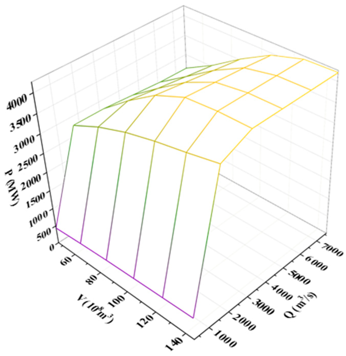
Figure 1. Approximate the hydropower output function by planes.
Energies 18 05102 g001
Figure 2. Gridding and definition.
Energies 18 05102 g002
Figure 3. Triangular gridding.
Energies 18 05102 g003
Figure 4. Geometric interpretation of subgradients of a concave function.
Energies 18 05102 g004
Figure 5. Non-concavity example (Three-Dimensional figure).
Energies 18 05102 g005
Figure 6. The error distribution of three models fit the testing function.
Energies 18 05102 g006aEnergies 18 05102 g006b
Figure 7. The RMSE by ARBLC with different gridding resolutions.
Energies 18 05102 g007
Figure 8. Comparison of three models on CPU time and RMSE.
Energies 18 05102 g008
Figure 9. Comparison of ARBLC and PWL1 on relative error distribution.
Energies 18 05102 g009
Figure 10. The RMSE and MAE by ARBLC with different gridding resolutions.
Energies 18 05102 g010aEnergies 18 05102 g010b
Table 1. Number of variables and constraints used for approximating the HOF through three models.
ModelConstraintsVariablesConstraints
ContinuousBinary
PWL1(24), (26), (27) 12 N 2 + 18 N + 9 4 N 2 + 8 N + 4 N 4 + 4 N 2 + 10 N + 5
TTBLC(29)–(32) 22 N 2 0 27 N 2 6 N + 7
ARBLC(24), (35) 11 N 2 0 N 4 + 3 N 2
Table 2. Results for the approximating test function through three models (CPU time and Rmse).
ModelsResolutions4163664100144196256324400
PWL1RMSE8.6762.1680.9150.5340.3400.2260.1650.128XX
MAE12.503.121.972.221.500.990.720.53XX
Time0.060.160.183.3311.4412.45293.12856.76XX
TTBLCRMSE14.5973.0481.2730.6910.4330.2950.2140.1630.1270.104
MAE22.695.532.491.390.890.620.450.350.270.22
Time0.080.180.110.110.150.170.280.260.360.48
ARBLCRMSE8.6762.1680.9640.5420.3460.2410.1770.1350.1070.085
MAE12.503.121.390.780.500.350.260.200.150.12
Time0.090.200.581.313.209.7319.3336.2466.28576.60
Table 3. The main characteristics of four large reservoirs in Lancang River [39].
CharacteristicsXiaowanManwanDachaoshanNuozhadu
OperabilityOver-yearyearlyyearlyOver-year
Minimum storage (108 m3)46.622.494.64104.425
Maximum storage (108 m3)145.573.7167.42217.776
Minimum release (m3/s)270280300800
Maximum release (m3/s)7600770077007900
Installed capacity (MW)4200167013505850
Disclaimer/Publisher’s Note: The statements, opinions and data contained in all publications are solely those of the individual author(s) and contributor(s) and not of MDPI and/or the editor(s). MDPI and/or the editor(s) disclaim responsibility for any injury to people or property resulting from any ideas, methods, instructions or products referred to in the content.