Article

Probabilistic HVAC Load Forecasting Method Based on Transformer Network Considering Multiscale and Multivariable Correlation

1
Southern Power Grid Research Institute Co., Ltd., Guangzhou 510663, China
2
Power Dispatch Control Center of Guangdong Power Grid Co., Ltd., Guangzhou 510600, China
*
Author to whom correspondence should be addressed.
Energies 2025, 18(19), 5073; https://doi.org/10.3390/en18195073
Submission received: 11 August 2025 / Revised: 11 September 2025 / Accepted: 16 September 2025 / Published: 24 September 2025
(This article belongs to the Topic Advances in Power Science and Technology, 2nd Edition)

Abstract

Accurate load forecasting for community-level heating, ventilation, and air conditioning (HVAC) plays an important role in determining an efficient strategy for demand response (DR) and the operation of the power grid. However, community-level HVAC includes various building-level HVACs, whose usage patterns and standard parameters vary, causing the challenge of load forecasting. To this end, a novel deep learning model, multiscale and cross-variable transformer (MSCVFormer), is proposed to achieve accurate community-level HVAC probabilistic load forecasting by capturing the various influences of multivariables on the load pattern, providing effective information for the grid operators to develop DR and operation strategies. This approach is combined with the multiscale attention (MSA) and cross-variable attention (CVA) mechanism, capturing the complex temporal patterns of the aggregated load. Specifically, by embedding the time series decomposition into the self-attention mechanism, MSA enables the model to capture the critical features of time series while considering the correlation between multiscale time series. Then, CVA calculates the correlations between the exogenous variable and aggregated load, explicitly utilizing the exogenous variables to enhance the model’s understanding of the temporal pattern. This differs from the usual methods, which do not fully consider the relationship between the exogenous variable and aggregated load. To test the effectiveness of the proposed method, two datasets from Germany and China are used to conduct the experiment. Compared to the benchmarks, the proposed method achieves outperforming probabilistic load forecasting results, where the prediction interval coverage probability (PICP) deviation with the nominal coverage and prediction interval normalized averaged width (PINAW) are reduced by 46.7% and 5.25%, respectively.

1. Introduction

The climate change problem in the 21st century, which is attributed to large amounts of CO2 emissions, has attracted much attention around the world which is attributed to large amounts of CO2 emissions [1,2]. Based on the statistical data of World Development Indicators from 1990 to 2020, the top five fossil fuel-consuming countries account for 55.43% of global CO2 emissions [3,4]. To solve the environmental problem and reduce the reliance on fossil fuels, the fuel consumption pattern conversion from fossil fuels to renewable energy is considered to be effective [5,6]. Meanwhile, recent research has found that improving the utilization proportion of renewable energy can mitigate the adverse influence of climate change [7]. In this context, more and more nations are commencing the reconfiguration of energy usage patterns, constructing low-carbon and sustainable cities. However, the generation characteristics of renewable energy, such as intermittency and low inertia, pose a challenge for the energy usage pattern conversion. Specifically, the intermittency implies a sharp fluctuation in the power supply in the power system [8]. The low inertia implies that the power system with high-penetration renewable energy will suffer a sharp reduction in voltage and frequency when the power shortage appears, damaging the stability of the power system. To this end, demand response (DR) provides a scalable solution, which adjusts the load demand of controllable loads to make the power demand adapt to the power supply fluctuation caused by the renewable energy, thereby ensuring the safety of the power system [9,10,11,12].
For these controllable loads participating in the DR, heating, ventilation, and air conditioning (HVAC) systems are the crucial appliances participating in the DR due to their unique characteristics. Their energy consumption occupies a large proportion of the building’s total consumption but could be effectively reduced by guiding HVAC to work in varying modes [13,14]. On the other hand, HVAC is utilized to improve the comfort level of the environment. According to the thermal inertia of a building, it can maintain the comfort level of the environment when HVAC is transferred into low energy consumption mode or turned off. For this characteristic, a large number of published studies have investigated effective control strategies and proved their enormous potential in reducing energy consumption [15,16,17]. Therefore, accurate energy consumption forecasting for HVAC in buildings is essential for constructing the power system with high-penetration renewable energy and mitigating the energy shortage and climate change problem [18,19], and it is the main research purpose in this paper.
Nowadays, the load forecasting of HVAC can be divided into two categories: the physical model-based method and the data-driven method. The physical model-based method is also called the white-box model, which constructs the mathematical model considering various variables, such as the temperature, the physical characteristics, and the occupancy rate, to calculate or forecast the HVAC load. This method provides great interpretation for the forecasting results [20]. However, the physical model is built based on some assumptions, which makes this model fail to reflect the real operation state of HVAC. Meanwhile, the physical model cannot capture the temporal pattern of HVAC, which leads to a low accuracy when an emergency appears [21,22]. With the development of smart meters and artificial intelligence, many researchers have investigated the employment of data-driven methods in HVAC load forecasting, which has low requirements for the building but analyzes the usage pattern of historical HVAC load. Ref. [23] utilized a temporal convolutional network (TCN) to construct the long-term temporality of HVAC load, thereby achieving determined load forecasting. Ref. [24] added the constraint of physical variables in the training of neural networks (NNs), enhancing their accuracy. Ref. [25] extended the HVAC load forecast from single-step forecasting to multi-horizon forecasting, conforming to the actual requirements for load forecasting. However, both the physical-based and data-driven methods focus on the building-level instead of the community-level load forecasting. For the community-level HVAC, because it includes HVACs from many households, where the usage pattern and standard parameters have some differences, analyzing its characteristics and forecasting its load accurately are challenging. Meanwhile, limited by the high cost of smart meters and the risk of privacy intrusion, it is difficult to acquire the measurements of HVAC.
To this end, some researchers have employed nonintrusive load monitoring (NILM), which decomposes the device load from the aggregated load, including varying the device load [26,27,28,29,30,31,32,33]. Ref. [29] combined multiple machine learning approaches, forecasting the state and load of HVAC. Ref. [30] employed a single processing technique in deep learning, decomposing the charge curve of an electric vehicle from the total electricity consumption. However, some research gaps exist, including the following:
(1)
Multiscale temporal patterns are commonly extracted, while the potential correlation between them remains unmodeled, limiting the capture of the accurate HVAC load fluctuation.
(2)
Exogenous variables are uniformly encoded by the NN, which neglects the intrinsic dependencies, preventing the modeling of complex HVAC load temporal patterns.
(3)
Probabilistic HVAC load forecasting is usually ignored in NILM, which is crucial for determining an efficient scheme of DR.
To this end, aiming at constructing a model that considers multiple factors, including the historical load data and exogenous variables, to forecast the HVAC load distribution in the future, this paper proposes the multiscale and cross-variable transformer (MSCVFormer). It employs the cross-variable attention (CVA) mechanism, capturing similar patterns between the exogenous variable and endogenous variable, thereby filtering potential patterns in the time series of the aggregated load series. To fully explore the temporality of time series, the multiscale attention (MSA) mechanism is used to handle load series with varying resolutions. Finally, the pinball loss is expanded to a multi-horizon pinball loss to achieve the prediction interval (PI) of HVAC, thereby evaluating the uncertainty of the predicted HVAC load. The main contributions of this research are as follows.
(1)
The MSA mechanism is proposed, which allows the model to capture the correlation between multiscale historical data. Specifically, it decomposes the historical data into multiple components with varying time scales, followed by single-scale and cross-scale attention mechanisms to capture their correlation and concretize them as attention scores. These attention scores enable the model to excavate the complex usage pattern of HVAC. This is in contrast to those models, which forecast the future data of each decomposition and obtain the prediction through addition.
(2)
The CVA mechanism is proposed, which enables the model to analyze the relevance between the exogenous variable patterns and HVAC load patterns. Specifically, it calculates the similarity of temporal patterns between the exogenous variables and aggregated load, which is further concretized as the weight matrix to extract the task-specific features from the aggregated load. Unlike conventional models that treat all input variables uniformly, the CVA mechanism explicitly considers the distinct temporal patterns, thereby preserving their unique predictive signatures.
(3)
The proposed model combines deep learning and quantile regression to achieve day-ahead probabilistic forecasting of the HVAC load. The parameters of the proposed model are optimized through the pinball loss, and the full load distribution of HVAC is learned by forecasting the multiple quantiles of HVAC simultaneously.

2. Problem Formulation

Multi-horizon HVAC probabilistic load forecasting aims to forecast the future HVAC load distribution through the historical load and exogenous variables, which can be formulated as Equation (1) [34,35].
y ^ q 1 , , y ^ q k , , y ^ q n T = f x | θ
where f ( | θ ) represents the mapping function of the MSCVFormer model. θ represents the MSCVFormer model’s parameters. Assume the time sequence x = { x 1 , , x l , , x L | x l d } as the input of the model, where the time length is L . For the features x l at each time stamp, it includes the historical data of the aggregated load and exogenous variables, formulated as x l and w l , respectively. w l = [ w l 1 , , w l d 1 ] represents d 1 exogenous variables. y ^ q 1 , , y ^ q k , , y ^ q n represent the predicted quantile sequence of the future HVAC load, where the number of quantiles is n . For the q k -th predicted quantile sequence, y ^ q k = [ y ^ L + 1 q k , y ^ L + 2 q k , , y ^ L + H q k ] , its time sequence length is H . Through the sliding window approach with a fixed-size window, the training and test sets are obtained, where the training set is used to optimize θ and the test set is used to evaluate the performance of the constructed model.

3. Methodology

As shown in Figure 1, the proposed method mainly includes two parts: variable selection, where the exogenous variables are used as the input of the MSCVFormer model, and the MSCVFormer. Their concrete content will be described in detail below.

3.1. Variable Selection

Historical load data are typically used to predict future load. However, in contrast to the conventional electricity load, the load patterns of HVAC also exhibit strong relevance to external environmental factors. For instance, high ambient temperatures often lead to lower temporary setpoints of HVAC, while high humidity levels may trigger increased use of ventilation modes. In this case, incorporating meteorological and environmental variables into the model can improve the forecasting accuracy. Nevertheless, not all potential input variables are strongly correlated with the HVAC load pattern. The variables with a weak correlation may introduce noise, which is harmful to the model’s performance. To address this issue, variable selection was conducted by calculating the Pearson Correlation Coefficient (PCC) [23,25], which detects the linear relationship between external variables and HVAC load. Meanwhile, the HVAC load at the same time stamp may exhibit a similar load distribution. Therefore, the Autocorrelation Coefficient (ACC) was also calculated to capture temporal dependencies in the historical load itself [36].
Specifically, the inputs of PCC and ACC are two time sequences. Their concrete calculation processes are as follows.
P C C = i = 1 m X i X ¯ ( Y i Y ¯ ) i = 1 m X i X ¯ 2 i = 1 m Y i Y ¯ 2
A C C = i = 1 m l a g X i X ¯ X i + l a g X ¯ i = 1 m X i X ¯ 2
where X i and Y i represent the i-th values of time sequences belonging to the HVAC load and external variable, respectively. X ¯ and Y ¯ represent the average value of the time sequence. m is the length of the time sequence. l a g is the time lag of the ACC. The range of PCC is from −1 to 1. When the absolute value of PCC is close to 1, it indicates a strong linear correlation between two variables. Otherwise, it indicates a weak linear correlation when the absolute value of PCC is close to 0. The range of ACC is from −1 to 1. When the absolute value of ACC is close to 1, it indicates an obvious periodicity pattern, such as the day-scale or week-scale periodicity, where the periodicity scale is equal to l a g . Through the calculation of PCC and ACC, the variables selected as the input of the model can be determined.

3.2. Multiscale and Cross-Variable Transformer

Figure 2 displays the architecture of the proposed model, MSCVFormer. It can be divided into three parts, including the MSA blocks capturing the complex temporal patterns of time series from the weather variables and the aggregated load, as well as the CVA blocks exploring the temporal pattern representation of the aggregated load, which is related to the weather variables. Finally, multiple multilayer perceptions are utilized to achieve the multi-horizon quantile regression.

3.2.1. Multiscale Attention Mechanism

To learn the complex temporal pattern of time series, multiple time series decompositions are employed, such as Empirical Mode Decomposition [37] and Seasonal and Trend Decomposition using Loess (STL) [38], which decompose the raw series into multiple sub-series and forecasts them, followed by the additive model or the multiplicative model to integrate the predictions. However, these separate predictions ignore the potential correlation between these sub-series. Even if these sub-series are handled by the NN simultaneously, they are treated equally and ignored in their relationship, which could affect the performance of the NN [38]. To explicitly capture the potential correlation between these sub-series and enable the model to focus on the critical information for the current task, the MSA Block is proposed, whose details are shown in Figure 3.
In the proposed network, multiple MSA blocks are cascaded to capture the temporal pattern of the time series. Assume the input of MSA blocks, X i , M S A , where X i , M S A B × L × d model . B represents the number of mini-batches. d model represents the length of the feature at each timestamp. Referring to the decomposition of STL, the average pool layer is utilized to produce the seasonal and trend components of the raw time series, regarded as X s e a s o n i , M S A and X t r e n d i , M S A and formulated as Equations (4) and (5), respectively. k s and k l represent the size of the averaging window, where k l is larger than k s . To keep the length of the features consistent, P a d d i n g is utilized to supply 0 at both ends of the input. The residual components, X r e s i d u a l i , M S A , are obtained through Equation (7). For the multiscale sub-series, C o n c a t , formulated as Equation (7), is utilized to concatenate them, thereby obtaining a comprehensive representation of the time series, X c o m p l e x i , M S A , where X c o m p l e x i , M S A B × L × 3 d model .
X s e a s o n i , M S A = AvgPool ( Padding ( X i , M S A ) , k e r n e l = k s )
X t r e n d i , M S A = AvgPool ( Padding ( X i , M S A ) , k e r n e l = k l )
X r e s i d u a l i , M S A = X i , M S A X s e a s o n i , M S A X t r e n d i , M S A
X c o m p l e x i , M S A = Concat ( X r e s i d u a l i , M S A , X s e a s o n i , M S A , X t r e n d i , M S A )
Then, the MSA mechanism is employed to explicitly calculate the pattern correlation between the sub-series, followed by picking up these critical features for the current task, which could be formulated as Equations (8) and (10). First, as shown in Equation (8), varying linear layers, including Dense Q ( ) , Dense K ( ) , and Dense V ( ) , are employed on X c o m p l e x i , M S A to produce different perspectives, including Q MSA , K MSA , and V MSA , respectively. These linear layers are learnable, thereby enhancing the learning capacity of the model. After that, the dot product between Q MSA and K MSA is calculated to obtain the attention score, assigning the large weights for these features, which are closely related to the current task. Different from the normal self-attention mechanism, the proposed MSA mechanism calculates the attention scores considering multiscale time series, explicitly exploring the correlation between the residual, seasonal, and trend components. By employing this mechanism on each component, the critical temporal pattern can be comprehensively captured, thereby enhancing the model’s learning capacity. In the end, as shown in Equation (10), the residual connection is utilized to improve the performance of the current task and avoid the performance degradation that usually appears in NNs with many layers.
Q MSA = Dense Q ( X c o m p l e x i , M S A ) K MSA = Dense K ( X c o m p l e x i , M S A ) V MSA = Dense V ( X c o m p l e x i , M S A )
Score = Softmax ( Q MSA K MSA T d model )
X o , M S A = Dense o ( Score × V MSA ) + X i , M S A

3.2.2. Cross-Variable Attention Mechanism

In load forecasting, due to the potential interactions with the load, exogenous variables like the weather are usually considered by the model to enhance its performance. For instance, in the estimation of photovoltaic generation, the radiation intensity and angle are used because their nonlinear relationship can be formulated as equations. In HVAC load forecasting, many exogenous variables have been investigated, such as the outdoor temperature, relative humidity, atmospheric pressure, and so on [37,39]. However, the data of these exogenous variables are usually handled equally with the HVAC load by the model, which may result in the degradation of the model since it ignores these exogenous variables and focuses on the historical load. To allow the model to mine the temporal patterns of these exogenous variables and construct their correlation with the HVAC load, the CVA mechanism is proposed, which explicitly extracts the sub-series from the aggregated load, while these sub-series have strong correlations with the exogenous variables.
Specifically, the function of the CVA mechanism can be formulated as Equations (11) and (13). In Equation (11), similar to the MSA mechanism, Q CVA , K CVA , and V CVA need to be produced according to the different linear layers. In this process, Q CVA is the linear projection of the time series W i , C V A from the exogenous variables, while the K CVA and V CVA are the linear projections of the time series X i , C V A from the aggregated load. Using Equation (12), the dot product between the Q CVA and K CVA is calculated, which displays the similarity between the time series from different variables, thereby allowing the model to evaluate the correlation between the HVAC load and the exogenous variables. This differs from the usual processing of exogenous variables, which just concatenates the time series from the exogenous variables and HVAC load, followed by the NN to analyze it. After that, this attention score is multiplied by V CVA , which captures the critical information V CVA related to exogenous variables, thereby facilitating the model learning of the complex pattern of the aggregated load.
Q CVA = Dense Q ( W i , C V A ) K CVA = Dense K ( X i , C V A ) V CVA = Dense V ( X i , C V A )
Score = Softmax ( Q CVA K CVA T d model )
X o , C V A = Dense o ( Score V CVA ) + X i , C V A

3.2.3. Multi-Horizon Quantile Regression

In a real-world scenario, multi-horizon forecasting is more practical than single-step forecasting. For instance, the strategies of DR or unit commitment for the next day will be determined by referring to day-ahead load forecasting results. Meanwhile, the biases between the prediction and ground truth are unavoidable. Accurate uncertainty estimation, which offers the PIs and ensures the ground truth is located within this interval, is crucial for certain fields when the safety of strategies is seriously considered. Therefore, multi-horizon probabilistic forecasting, providing the predictions and their uncertainty, is necessary. In this research, the pinball loss is used to achieve probabilistic forecasting, whose formulation is shown in Equation (14).
L i , q k , h ( y h i , y ^ h i , q k ) = ( 1 q k ) ( y ^ h i , q k y h i ) i f y ^ h i , q k y h i q k ( y h i y ^ h i , q k ) i f y ^ h i , q k y h i
where y h i represents the label of x i at the h -th forecasting horizon. This loss function lets the model predict multiple quantiles of the sample x i . q k is set to varying values, thereby allowing the model to capture the entire PI. To expand it to multi-horizon probabilistic forecasting, the output layer of the model is adjusted according to Figure 2. Multiple linear layers are employed, where the number of linear layers is equal to the number of target quantiles. Combined with the backpropagation, the parameters of the NN are optimized, as shown in Equation (15).
θ = arg min θ i I h [ L , L + H ] q k [ q 1 , , q n ] L i , q k , h ( y h i , y ^ h i , q k )
where θ represents the parameters of the NN. I represents the sample index in the training set. When q k is equal to 50, it could be viewed as the determined prediction.

4. Case Study

4.1. Dataset Setup

Two datasets were used to conduct the experiments, including the WPuQ dataset [40] and the EnergyDetective2020 dataset [41]. Specifically, the WPuQ dataset collected the electricity consumption of whole households and thermal appliances from some households in the same community. The collection period was from 2018 to 2020 with a 1 h time resolution. Due to the missed measurements, 21 households, whose measurements exceeded 90%, were selected for this experiment. The sum of their whole household electricity consumption was used as the aggregated load, while the sum of their thermal appliance electricity consumption was used as the HVAC load. Figure 4 shows the curve of the aggregated load. It can be observed that the energy demand in the winter season is higher than in the summer season. Apart from the aggregated load and HVAC load, the WPuQ dataset also provides the measurements of exogenous variables, including apparent temperature (AT), atmospheric pressure (AP), relative humidity (RH), solar irradiance (SI), and wind speed (WS). Through the calculation of PCC and ACC, the exogenous variables strongly related to HVAC load and the periodicity pattern of HVAC can be obtained, whose concrete values are shown in Figure 5. According to the content of Figure 5a, the AT has a strong relationship with HVAC, while other exogenous variables have a weak one. Therefore, the AT was utilized in the HVAC load forecasting. Furthermore, according to the content of Figure 5b, the HVAC load displays strong periodicity in the time scales of one day and one week. Therefore, the timestamp was utilized in the HVAC load forecasting.
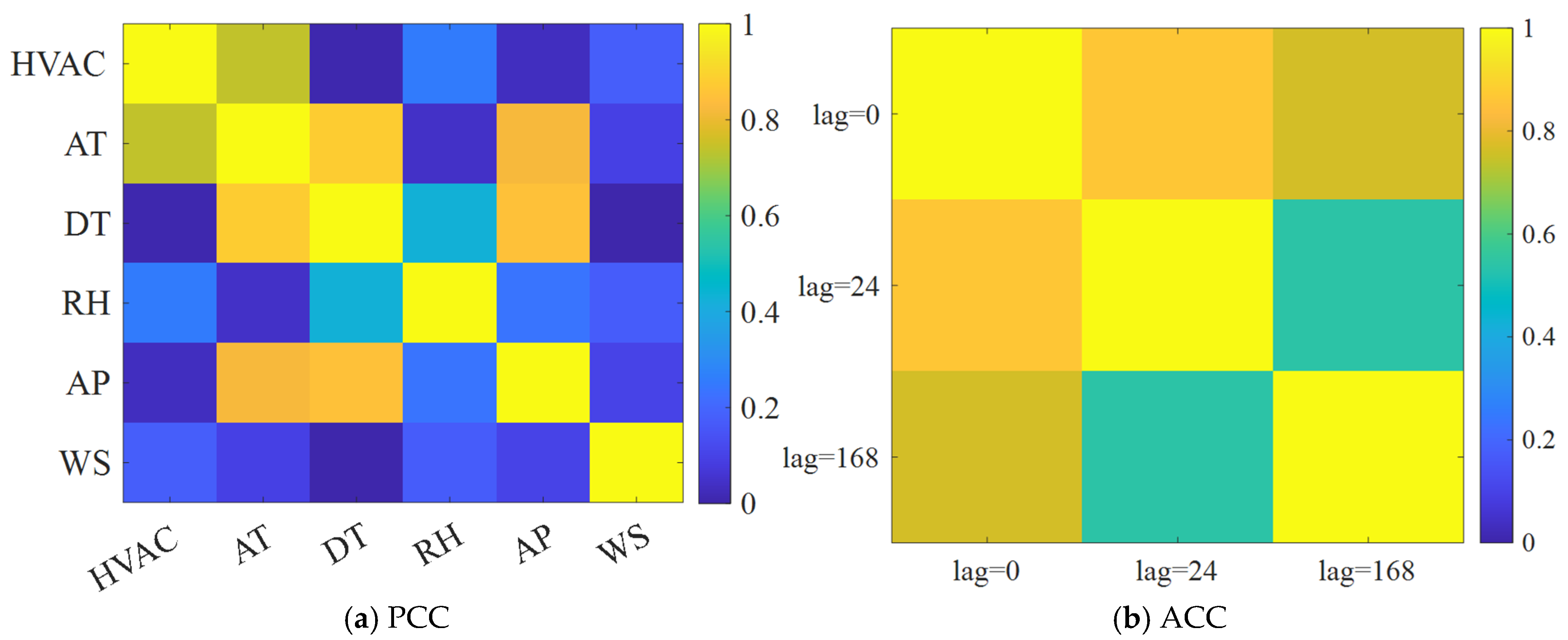
The EnergyDetective2020 dataset collected the electricity consumption of 20 office buildings in Shanghai, which includes the HVAC load and the light and socket load, respectively. The collection period was from 2015 to 2017 with a 1 h time resolution. Four buildings were categorized into the same community, whose electricity consumption sum is regarded as the aggregated load. Their HVAC load sum is regarded as the HVAC load. Figure 6 shows the curve of aggregated load. It can be observed that the energy demand in the winter season is higher than in the summer season. Apart from the aggregated load and HVAC load, the EnergyDetective2020 dataset also provides the measurements of exogenous variables, including AT, Dew Point Temperature (DT), RH, AP, and WS. Their PCC and ACC results are shown in Figure 7. Similar to the WPuQ dataset, the HVAC load exhibits strong correlation with AT, as well as the periodicity patterns in the time scales of one day and one week. Therefore, the historical data of AT and timestamps were used in the HVAC load forecasting.
Four cases of each dataset are considered to simulate various seasons. The detailed ranges of the training set, test set, and validation set of the WPuQ and EnergyDetective2020 datasets are shown in Table 1. The selected variables include the following: (1) the historical aggregated load; (2) the historical AT data; and (3) the timestamps, including the day and week. In the training phase, the training set is utilized to optimize the model parameters, while the validation set is used to adjust the hyperparameters. In the test phase, the test set is employed to evaluate the performance of the trained model. The values of d , L , and H are set as 3, 48, 24.

4.2. Evaluation Metrics

To evaluate the performance of determined forecasting results and probabilistic forecasting results, four widely used metrics are utilized in this study [42,43,44,45].
(1)
Metrics for deterministic forecasting
The Root Mean Squared Error (RMSE) and Mean Absolute Percentage Error (MAPE) are used to evaluate deterministic forecasting.
RMSE = 1 m H i = 1 m h = 1 H y ^ h i y h i 2
MAPE = 1 m H i = 1 m h = 1 H | y ^ h i y h i | | y h i |
where m represents the number of samples. A lower RMSE and MAPE indicate a better performance of deterministic forecasting.
(2)
Metrics for probabilistic forecasting
Prediction interval coverage probability (PICP) and prediction interval normalized averaged width (PINAW) are utilized to evaluate probabilistic forecasting.
PICP = 1 m H h = 1 H i = 1 m I L h i y ^ h i U h i
I L h i y ^ h i U h i = 1 ,   i f   L h i y ^ h i U h i 0 ,   e l s e
PINAW = 1 m R h = 1 H i = 1 m U h i L h i
where U h i and L h i h represents the upper and lower bounds of the PIs constructed for the i -th samples at the h -th forecasting horizon. R represents the range of y i . When PICP is close to the confidence level α , it indicates that the model can accurately capture the forecasting uncertainty. When PINAW is smaller, it indicates the low forecasting uncertainty of the model.

4.3. Baseline and Benchmark

(1)
Baseline
The persistent model (PM) is regarded as the baseline, which utilizes the load of the previous day as the predicted future load. However, the model is fed with the total load instead of the HVAC load, where these two kinds of load have some differences. Therefore, the percentage between the HVAC load and the total load in each season is calculated, which is regarded as the coefficient that is multiplied by the predicted total load to obtain the HVAC load.
(2)
Benchmark
One machine learning-based and three deep learning-based models, including gradient boosting regressor (GBR), bidirectional long and short-term memory (BiLSTM), Convolutional Neural Network (CNN)-LSTM, and Transformer, which are usually utilized in load forecasting, are regarded as the benchmarks.
GBR [46]: This is a machine learning algorithm based on ensemble learning. It builds multiple weak regressors, followed by analyzing their predicted results to obtain excellent performance.
BiLSTM [24]: This is a deep learning algorithm that focuses on time series forecasting. It explicitly analyzes the temporal patterns through sequential processing, thereby accurately predicting the load.
CNN-LSTM [28]: This is a deep learning algorithm. Before the features are fed into the LSTM, a CNN is employed on the samples to first extract the features at each timestamp.
Transformer [18]: Its structure is similar to CNN-LSTM, while the section of LSTM is replaced with a Transformer Encoder.
Autoformer [47]: This is an advanced Transformer-based deep learning algorithm. It combines the autocorrelation mechanism and series decomposition to extract the complex temporal features of the input. The hyperparameters of these benchmarks are shown in Table 2. The structure of the proposed method is shown in Table 3.
To achieve probabilistic forecasting, each deep learning-based method is optimized to forecast 19 quantiles, where the values of the quantile are [ 5 ,   10 ,   15 ,   ,   95 ] . When GBR is employed in each case, 456 GBRs are built, i.e., 19 GBRs for each step corresponding to 19 quantile regressor problems. For determined forecasting, their forecasting results when the quantile is 50 are utilized to evaluate their performance.

4.4. Determined Forecasting

4.4.1. Results

Table 4 lists the deterministic forecasting results of MSCVFormer and other benchmark methods on two datasets, WPuQ and EnergyDetective2020. For their performance on the WPuQ dataset, it can be observed that MSCVFormer can obtain competitive RMSE and MAPE, outperforming these basic and advanced deep learning-based methods, such as BiLSTM, Transformer, and Autoformer. Specifically, compared to other comparative methods, MSCVFormer reduces the RMSE by 1.67% and 3.13% in Case 1 and Case 4, respectively. Similarly, for the EnergyDetective2020 dataset, MSCVFormer achieves the best performance, reducing the RMSE by 9.47%, 12.34%, 15.54%, and 12.75% and reducing the MAPE by 9.06%, 14.14%, 7.97%, and 4.10%. In summary, MSCVFormer exhibits an excellent deterministic load forecasting ability for the HVAC load.
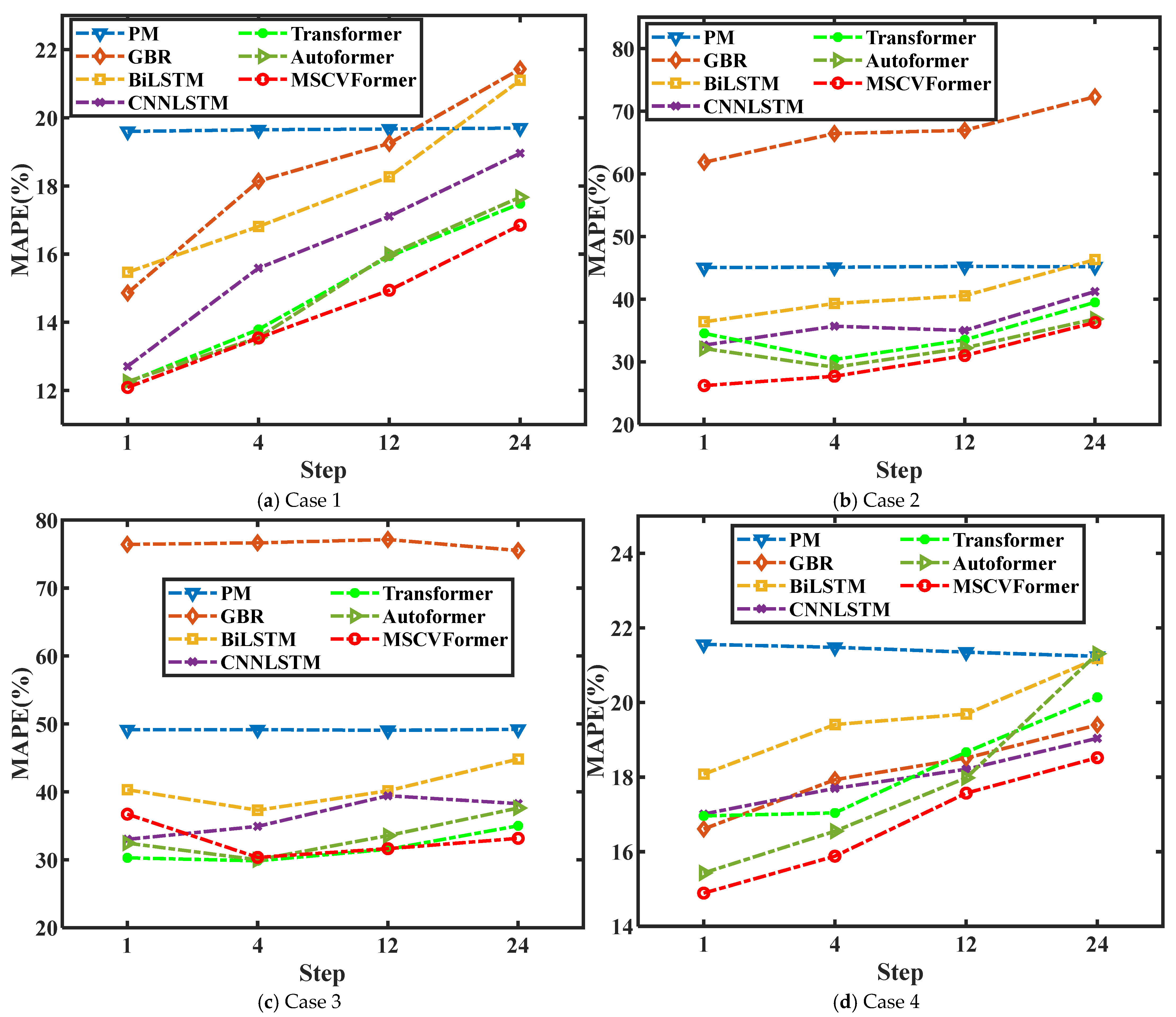
Furthermore, its deterministic load forecasting ability is explored at different forecasting horizons. The MAPEs of MSCVFormer and other benchmark models at varying forecasting horizons on the WPuQ dataset are plotted in Figure 8. It can be observed that MSCVFormer obtains worse performance when the forecasting horizon increases. Meanwhile, compared to these benchmark models, MSCVFormer achieves the optimal forecasting results at each forecasting horizon. To this end, MSCVFormer possesses a superior ability for accurate HVAC load forecasting for a longer forecasting horizon.

4.4.2. Discussion of the Results

As the baseline method, PM is used to test the task difficulty. Its unsatisfactory performance is derived from the complex load pattern of HVAC, where the ratio of the HVAC load to the aggregated load is random, which conflicts with the load forecasting method of PM, using the fixed ratio and the aggregated load to calculate the HVAC load. For GBR, relying on its decision tree to capture the nonlinear correlation between the aggregated load and HVAC load, it achieves an improved performance in most cases. However, due to the limited learnable parameters and feature extraction, its performance fails to match these deep learning-based models. Through the employment of LSTM, which analyzes the time series sequentially, BiLSTM and CNN-LSTM can capture the short-term and long-term temporal patterns but fail to capture the correlation between two features with long time intervals. In contrast to the LSTM, due to the self-attention mechanism, the Transformer can directly calculate the correlation between any two features. Its flexibility provides the paths for Transformer-based models to capture the task-specific features and achieve better HVAC load forecasting. Meanwhile, its multi-head attention mechanism further enables the model to obtain various features and construct a comprehensive understanding of the HVAC load. Nevertheless, MSCVFormer still achieves an improved performance compared to these Transformer-based methods, where the improvements in performance are significant on the EnergyDetective2020 datasets. This is because MSCVFormer can utilize the CVA block to individually analyze the fluctuation pattern of different variables, calculating the specific influence of external variables on the aggregated load, thereby ensuring the effective utilization of these external variables in understanding the HVAC load. Meanwhile, MVA blocks ensure that the proposed model captures the load pattern from the multiscale time series, where the tendency and fluctuation of the HVAC load assist the model in achieving better HVAC load forecasting at the long forecasting horizon.

4.5. Probabilistic Forecasting

4.5.1. Results

Table 5 displays the probabilistic load forecasting results when the confidence level is 90%. According to the experimental results, MSCVFormer achieves superior performance across all cases on both datasets, particularly in terms of PINAW, while maintaining high PICP values. On the WPuQ dataset, MSCVFormer consistently achieves low PINAW values in most cases, indicating narrower PIs compared to other methods, where PINAW values are reduced by 9.42% and 3.97% in Case 1 and Case 3, respectively. In Case 2 and Case 4, while the PINAWs of MSCVFormer are slightly higher than those of Autoformer, a competitive PICP is obtained, where the deviations between the PICP and the nominal confidence level are 0.01 and 0.003, which are lower than those of Autoformer. Notably, MSCVFormer overall outperforms Transformer and Autoformer. Furthermore, on the EnergyDetective2020 dataset, only MSCVFormer and Transformer achieve lower PINAW values in all four cases, whose PINAW is lower than 0.01, significantly outperforming other models. However, compared to Transformer, MSCVFormer obtains a higher PICP, where the deviations in the PICP with the nominal confidence level are 0.006, 0.019, 0.025, and 0.027. In summary, MSCVFormer can deliver accurate PIs with a narrow interval width and reliable coverage.
Considering that both Transformer and MSCVFormer can provide high-quality PIs with a high PICP and low PINAW when the nominal confidence is set to 90%, another experiment was conducted to compare their performance in implementing probabilistic HVAC load forecasting when the nominal confidence is set to 60%, 70%, 80%, and 90%. Figure 9 shows the PICP of these two methods in different cases. It can be observed that the proposed method can provide a PICP that matches the nominal confidence level in Case 2, Case 3, and Case 4, which is significantly better than the performance of the Transformer, which obtains a PICP with a large bias from the nominal confidence level [48]. This indicates that the proposed method can capture the uncertainty of model predictions to a limited extent in most cases and generate PIs of an appropriate width to cover these true values, providing effective information for formulating feasible DR strategies.
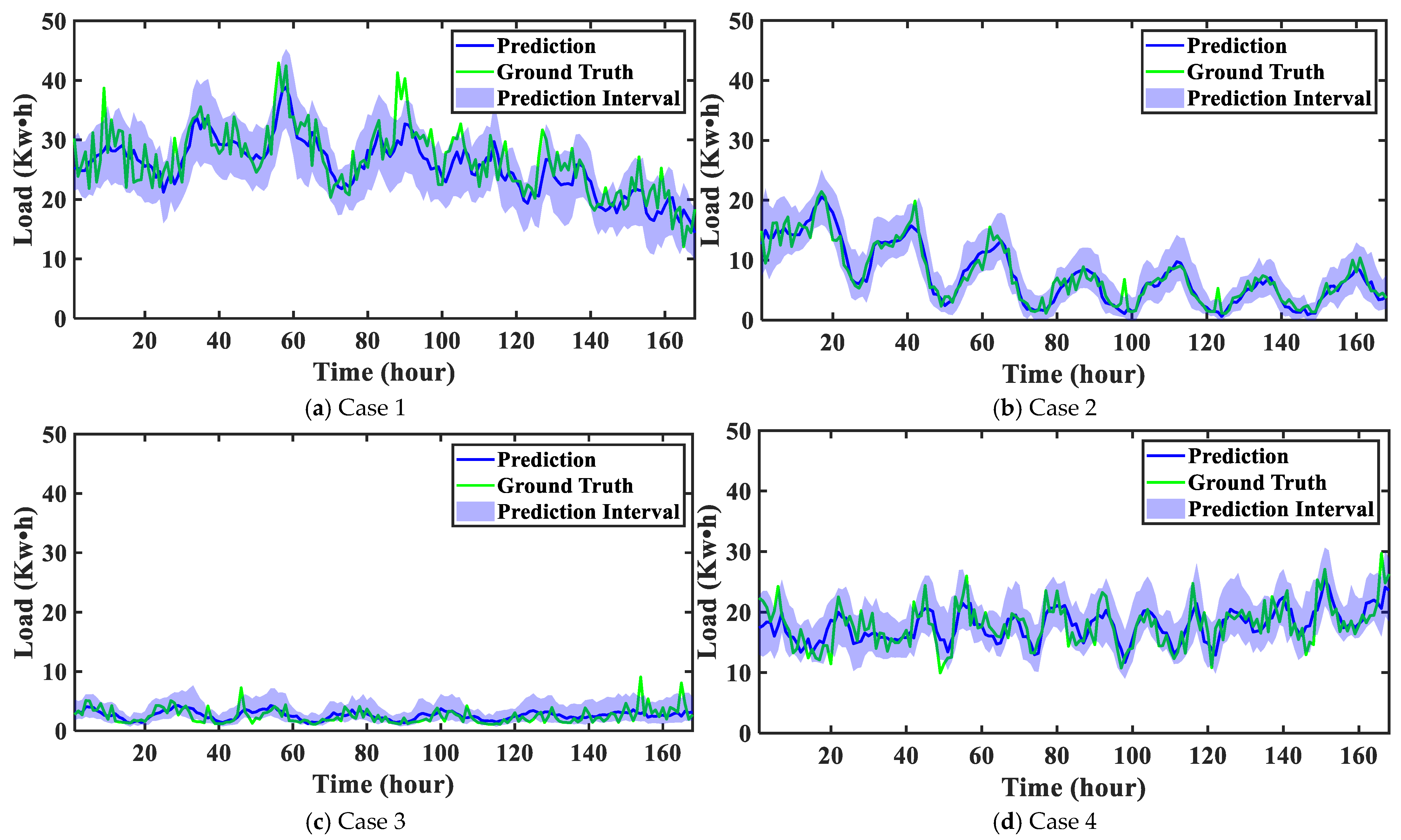
To directly demonstrate the performance of the proposed method in probabilistic HVAC load forecasting, Figure 10 shows the PIs of one week of each case on the WPuQ dataset. These weeks are randomly selected. It can be observed that significant differences in the range of HVAC loads in different cases exist, with the load range being [10, 40] in Case 1 and [0, 10] in Case 3. At the same time, there are differences in their load patterns. For example, in Case 1 and Case 2, the HVAC load shows a decreasing trend. For different HVAC load modes, the proposed method can provide a PI with an adaptive interval width, which is narrower in Case 3 and wider in Case 1. At the same time, these PIs can cover the vast majority of HVAC loads. To this end, the proposed method can ensure that the model outperforms probabilistic forecasting.

4.5.2. Discussion of the Results

Among these benchmark models in Table 5, GRB exhibits an unstable probabilistic load forecasting performance on both datasets, as evident from a significant gap between its PICP and nominal confidence level. This is because the construction of multiple GBRs is required to achieve probabilistic HVAC load forecasting, with each GBR predicting a percentile separately. This approach prevents GBR from learning the complete HVAC load distribution using the same set of parameters, resulting in lower robustness, i.e., an unstable PICP. Unlike GBR, these deep learning-based models are combined with quantile regression, where their output is no longer a single deterministic prediction, but rather multiple quantiles, which prompts the model to perceive prediction uncertainty and provide effective PIs. However, the sharpness and coverage of the constructed PIs still depend on the ability to capture complex HVAC load patterns. For BiLSTM and CNN-LSTM, these two basic deep learning-based models, as analyzed in Section 4.4.2, fail to provide optimal deterministic HVAC load forecasting, which means they have higher prediction uncertainty and require higher interval widths to ensure sufficient coverage of the intervals. The advanced Transformer-based model, Autoformer, achieves better probability prediction performance compared to Transformer on the EnergyDetective2020 dataset, providing PIs with a higher PICP. This is due to its strong ability to extract periodic features, as well as its autocorrelation attention mechanism, which automatically analyzes potential periodicity in the input and achieves tailored modeling, thereby resulting in a better performance on the aggregated load with a strong periodicity, such as EnergyDetective2020. Compared to Autoformer, MSCVFormer can construct the PI with enough PICP and a narrow interval width on both datasets. This benefits from the utilization of CVA, which integrates the fluctuation degrees of various external variables and aggregated loads, enabling the accurate prediction of the load distribution of HVAC. Meanwhile, MSA decomposes the time series into components of different time scales, which assists the model in accurately perceiving the degree of fluctuation of these variables, thus laying a solid foundation for achieving accurate probabilistic HVAC load forecasting.

5. Discussion

5.1. Application

The proposed method allows for accurate HVAC load probabilistic forecasting, which provides the critical support for DR and the energy management of the power grid. Specifically, it can be used to evaluate the potential ability of HVAC systems to participate in DR and to make energy scheduling more economic and resilient due to the accurate load distribution forecasting.

5.2. Limitations

The proposed method assumes that large amounts of HVAC load at the initial training phase are available, while they are impractical for the newly constructed building and community. In this case, it is a challenge to utilize even fewer zero samples to achieve accurate HVAC load forecasting.

6. Conclusions

This article proposes a novel data-driven method, MSCVFormer, to predict the HVAC load of the next day based on the historical data of aggregated load and exogenous variables. In this process, through the PCC and the ACC, the temperature and timestamp are utilized in the HVAC load forecasting. MSCVFormer includes two novel blocks to extract the complex temporal pattern of time series. Specifically, MSA is proposed, embedding the STL into the self-attention mechanism. This design enables the NN to focus on the pattern correlation between multiscale time series, thereby capturing the critical information for HVAC load forecasting. This is in contrast to the conventional methods, which separately conduct the feature extraction and prediction for each component of the input, ignoring their correlation. Meanwhile, CVA is proposed, calculating the similarity between the time series from different variables, thereby achieving the essential feature extraction. Unlike conventional models that treat all input variables uniformly, this block innovatively considers the differences between varying variables, thereby efficiently utilizing these exogenous variables to assist the model in capturing the complex temporal pattern of the load. Compared to the advanced Transformer-based methods, such as Autoformer, which employs the series decomposition and delayed aggregation, the proposed method has better performance in deterministic forecasting, where the RMSE and MAPE are reduced by 13.04% and 8.81% on average on the WPuQ and EnergyDetective2020 datasets, respectively. Meanwhile, the proposed method can deliver the PIs with a PICP close to the nominal confidence intervals and reduce the interval width by 43.89% compared to Autoformer on the EnergyDetective2020 dataset.

Author Contributions

Conceptualization, T.P. and Z.Z.; methodology, H.L.; software, C.L.; validation, X.J., C.L. and Z.Z.; formal analysis, Z.M.; investigation, X.C.; resources, X.C.; data curation, T.P.; writing—original draft preparation, X.J.; writing—review and editing, H.L.; visualization, C.L.; supervision, T.P.; project administration, Z.M. All authors have read and agreed to the published version of the manuscript.

Funding

This work was supported by the Southern Power Grid Corporation Technology Project under Grant 036000KK52222004(GDKJXM20222117).

Data Availability Statement

The original contributions presented in this study are included in the article; further inquiries can be directed to the corresponding author.

Conflicts of Interest

Authors Tingzhe Pan, Hongxuan Luo and Xin Jin were employed by the Southern Power Grid Research Institute Co., Ltd. Zean Zhu, Chao Li, Zijie Meng and Xinlei Cai were employed by the Power Dispatch Control Center of Guangdong Power Grid Co., Ltd. The authors declare that the research was conducted in the absence of any commercial or financial relationships that could be construed as a potential conflict of interest.

Abbreviations

Symbol
f · The mapping function
θ The parameters of f ·
x The time sequence input into the model
L The length of x
x l The feature of x at the l -th time stamp
x l The historical data of the aggregated load in x l
w l i The historical data of exogenous variables in x l
w l d 1 The ( d 1 ) -th exogenous variables in w l i
d The number of variables, including the aggregated load and exogenous variables
y ^ q k The q k -th predicted quantile of the future HVAC load
H The forecasting horizon of the future HVAC load
y ^ L + H q k The q k -th predicted quantile at the L + H -th forecasting horizon
B The batch size
x i The i -th sample
y h i The label of the i -th sample at the h -th forecasting horizon
y ^ i , q k The q k -th predicted quantile sequence of the i -th sample
I The sample index set
X i , M S A The input of the MSA block
X t r e n d i , M S A The tendency components of X i , M S A through the STL
X s e a s o n i , M S A The seasonal components of X i , M S A through the STL
X r e s i d u a l i , M S A The seasonal residual of X i , M S A through the STL
X c o m p l e x i , M S A The complex feature representation of X i , M S A
d model The feature length of the input
Q MSA The query matrix of the MSA block
K MSA The key matrix of the MSA block
V MSA The value matrix of the MSA block
X o , M S A The output of the MSA block
X i , C V A The aggregated load sequence input of the CVA block
W i , C V A The exogenous variable sequence input of the CVA block
Q CVA The query matrix of the CVA block
K CVA The key matrix of the CVA block
V CVA The value matrix of the CVA block
X o , C V A The output of the CVA block
U h i The upper bound of the PI of the i -th sample at the h -th forecasting horizon
L h i The lower bound of the PI of the i -th sample at the h -th forecasting horizon
l a g The time lag of ACC
Abbreviation
MSCVFormerMultiscale and Cross-Variable Transformer
NILMNonintrusive Load Monitoring
HVACHeating, Ventilation, and Air Conditioning
DRDemand Response
STLSeasonal and Trend Decomposition using Loess
TCNTemporal Convolutional Network
NNNeural Network
CNNConvolutional Neural Network
LSTMLong and Short-Term Memory
MSAMultiscale Attention
CVACross-Variable Attention
PCCPearson Correlation Coefficient
ACCAutocorrelation Coefficient
PIPrediction Interval
MAPEMean Absolute Percentage Error
RMSERoot Mean Square Error
PICPPrediction Interval Coverage Probability
PINAWPrediction Interval Normalized Averaged Width
PMPersistent Model
GBRGradient Boosting Regressor
BiLSTMBidirectional LSTM

References

  1. Groll, M. Can Climate Change Be Avoided? Vision of a Hydrogen-Electricity Energy Economy. Energy 2023, 264, 126029. [Google Scholar] [CrossRef]
  2. Carlini, F.; Christensen, B.J.; Gupta, N.D.; de Magistris, P.S. Climate, Wind Energy, and CO2 Emissions from Energy Production in Denmark. Energy Econ. 2023, 125, 106821. [Google Scholar] [CrossRef]
  3. WDI. World Development Indicators Data Bank [WWW Document]. 2023. Available online: https://databank.worldbank.org/source/world-development-indicators (accessed on 22 October 2023).
  4. Rahman, A.; Murad, S.M.W.; Mohsin, A.K.M.; Wang, X. Does Renewable Energy Proactively Contribute to Mitigating Carbon Emissions in Major Fossil Fuels Consuming Countries? J. Clean. Prod. 2024, 452, 142113. [Google Scholar] [CrossRef]
  5. Al-Ghussain, L.; Alrbai, M.; Al-Dahidi, S. Comprehensive Techno-Economic and Life Cycle Greenhouse Gases Analysis of Green Ammonia Production Utilizing PV and Wind Energy: Jordan as a Case Study. Renew. Energy 2025, 249, 123249. [Google Scholar] [CrossRef]
  6. Alvi, S.; Ahmad, I.; Nawaz, S.M.N.; Connell, W.; Anser, M.K.; Hassan, M.U. The Role of Green Finance, Energy Transition, and Digitalization in OECD Greenhouse Gas Emissions. J. Clean. Prod. 2025, 518, 145865. [Google Scholar] [CrossRef]
  7. Sadiq, M.; Nawaz, M.A.; Chien, F.; Sharif, A.; Hanif, S. Enhancing Environmental Quality and Mitigating Climate Change: A Renewable Energy Policy Perspective Based on Evidence from Most Polluted European Countries. Gondwana Res. 2025, 148, 96–105. [Google Scholar] [CrossRef]
  8. Johnathon, C.; Agalgaonkar, A.P.; Planiden, C.; Kennedy, J. A Proposed Hedge-Based Energy Market Model to Manage Renewable Intermittency. Renew. Energy 2023, 207, 376–384. [Google Scholar] [CrossRef]
  9. Ercoli, P.; Mugnini, A.; Arteconi, A. Demand Response for Renewable Energy Communities: Exploring Coordination of Prosumer-Generated PV and Flexible Aggregated Demand in the Italian Framework. Energy Build. 2025, 340, 115814. [Google Scholar] [CrossRef]
  10. Cao, D.; Hu, W.; Zhao, J.; Zhang, G.; Zhang, B.; Liu, Z.; Chen, Z.; Blaabjerg, F. Reinforcement Learning and Its Applications in Modern Power and Energy Systems: A Review. J. Mod. Power Syst. Clean Energy 2020, 8, 1029–1042. [Google Scholar] [CrossRef]
  11. Cao, D.; Zhao, J.; Hu, J.; Pei, Y.; Huang, Q.; Chen, Z.; Hu, W. Physics-Informed Graphical Representation-Enabled Deep Reinforcement Learning for Robust Distribution System Voltage Control. IEEE Trans. Smart Grid 2024, 15, 233–246. [Google Scholar] [CrossRef]
  12. Zhao, P.; Hu, W.; Cao, D.; Huang, R.; Wu, X.; Huang, Q.; Chen, Z. Causal Mechanism-Enabled Zero-Label Learning for Power Generation Forecasting of Newly-Built PV Sites. IEEE Trans. Sustain. Energy 2025, 16, 392–406. [Google Scholar] [CrossRef]
  13. Change, I.P. Climate Change 2014: Mitigation of Climate Change: Working Group III Contribution to the IPCC Fifth Assessment Report; Cambridge University Press: Cambridge, UK, 2015. [Google Scholar] [CrossRef]
  14. China Building Energy Consumption Annual Report 2020. Build. Energy Effic. 2021, 2, 1–6. Available online: https://lib.cqvip.com/Qikan/Article/Detail?id=7104165988 (accessed on 6 September 2025).
  15. Talib, R.; Nassif, N. “Demand Control” an Innovative Way of Reducing the HVAC System’s Energy Consumption. Buildings 2021, 11, 488. [Google Scholar] [CrossRef]
  16. Azuatalam, D.; Lee, W.-L.; de Nijs, F.; Liebman, A. Reinforcement Learning for Whole-Building HVAC Control and Demand Response. Energy AI 2020, 2, 100020. [Google Scholar] [CrossRef]
  17. Yu, L.; Jiang, T.; Zou, Y. Online Energy Management for a Sustainable Smart Home With an HVAC Load and Random Occupancy. IEEE Trans. Smart Grid 2019, 10, 1646–1659. [Google Scholar] [CrossRef]
  18. Alden, R.E.; Gong, H.; Jones, E.S.; Ababei, C.; Ionel, D.M. Artificial Intelligence Method for the Forecast and Separation of Total and HVAC Loads With Application to Energy Management of Smart and NZE Homes. IEEE Access 2021, 9, 160497–160509. [Google Scholar] [CrossRef]
  19. Wang, H.; Mai, D.; Li, Q.; Ding, Z. Evaluating Machine Learning Models for HVAC Demand Response: The Impact of Prediction Accuracy on Model Predictive Control Performance. Buildings 2024, 14, 2212. [Google Scholar] [CrossRef]
  20. Afram, A.; Janabi-Sharifi, F. Review of Modeling Methods for HVAC Systems. Appl. Therm. Eng. 2014, 67, 507–519. [Google Scholar] [CrossRef]
  21. Nomura, A.; Shi, S.; Miyata, S.; Akashi, Y.; Momota, M.; Sawachi, T. Design–Operation Gap Caused by Parameter Variance in HVAC System Control Sequences: A Simulation-Based Study on Energy Efficiency and Temperature Controllability. J. Build. Eng. 2024, 87, 109112. [Google Scholar] [CrossRef]
  22. Zhao, H.; Magoulès, F. A Review on the Prediction of Building Energy Consumption. Renew. Sustain. Energy Rev. 2012, 16, 3586–3592. [Google Scholar] [CrossRef]
  23. He, N.; Zhang, L.; Qian, C.; Gao, F.; Li, R.; Cheng, F.; Chu, D. Short-Term Cooling Load Prediction for Central Air Conditioning Systems with Small Sample Based on Permutation Entropy and Temporal Convolutional Network. Energy Build. 2024, 310, 114115. [Google Scholar] [CrossRef]
  24. Wang, Y.; Zhan, C.; Li, G.; Zhang, D.; Han, X. Physics-Guided LSTM Model for Heat Load Prediction of Buildings. Energy Build. 2023, 294, 113169. [Google Scholar] [CrossRef]
  25. Yu, H.; Zhong, F.; Du, Y.; Xie, X.; Wang, Y.; Zhang, X.; Huang, S. Short-Term Cooling and Heating Loads Forecasting of Building District Energy System Based on Data-Driven Models. Energy Build. 2023, 298, 113513. [Google Scholar] [CrossRef]
  26. Gopinath, R.; Kumar, M. DeepEdge-NILM: A Case Study of Non-Intrusive Load Monitoring Edge Device in Commercial Building. Energy Build. 2023, 294, 113226. [Google Scholar] [CrossRef]
  27. Kulathilaka, M.J.S.; Saravanan, S.; Kumarasiri, H.D.H.P.; Logeeshan, V.; Kumarawadu, S.; Wanigasekara, C. NILM for Commercial Buildings: Deep Neural Networks Tackling Nonlinear and Multi-Phase Loads. Energies 2024, 17, 3802. [Google Scholar] [CrossRef]
  28. Sun, X.; Hu, J.; Hu, W.; Cao, D.; Chen, Z.; Blaabjerg, F. Non-Intrusive Load Monitoring Based on Process-Adaptive Multi-Target Regression and Transformer-Enabled Two-Stream Input Network. Appl. Energy 2025, 393, 126046. [Google Scholar] [CrossRef]
  29. Botman, L.; Lago, J.; Fu, X.; Chia, K.; Wolf, J.; Kleissl, J.; De Moor, B. Building Plug Load Mode Detection, Forecasting and Scheduling. Appl. Energy 2024, 364, 123098. [Google Scholar] [CrossRef]
  30. Kianpoor, N.; Hoff, B.; Østrem, T.; Yousefi, M. Home Energy Management System for a Residential Building in Arctic Climate of Norway Using Non-Intrusive Load Monitoring and Deep Learning. IEEE Trans. Ind. Appl. 2024, 60, 5589–5598. [Google Scholar] [CrossRef]
  31. Sun, X.; Hu, J.; Hu, W.; Cao, D.; Chen, J.; Zhang, Z.; Chen, Z.; Blaabjerg, F. Pattern Consistency Learning-Enabled Nonintrusive Load Monitoring Considering Limited Appliance Annotations. IEEE Trans. Instrum. Meas. 2025, 74, 2534013. [Google Scholar] [CrossRef]
  32. Yang, X.; Zhang, L.; Zhao, H.; Zhang, W.; Long, C.; Wu, G.; Zhao, J.; Shen, X. Multi-Level Decomposition and Interpretability-Enhanced Air Conditioning Load Forecasting Study. Energies 2024, 17, 5881. [Google Scholar] [CrossRef]
  33. Massidda, L.; Marrocu, M. Total and Thermal Load Forecasting in Residential Communities through Probabilistic Methods and Causal Machine Learning. Appl. Energy 2023, 351, 121783. [Google Scholar] [CrossRef]
  34. Zhou, H.; Zhang, S.; Peng, J.; Zhang, S.; Li, J.; Xiong, H.; Zhang, W. Informer: Beyond Efficient Transformer for Long Sequence Time-Series Forecasting. In Proceedings of the AAAI Conference on Artificial Intelligence, Virtual Event, 2–9 February 2021; Volume 35, pp. 11106–11115. [Google Scholar] [CrossRef]
  35. Hart, G.W. Nonintrusive Appliance Load Monitoring. Proc. IEEE 1992, 80, 1870–1891. [Google Scholar] [CrossRef]
  36. Huang, N.; Hu, Z.; Cai, G.; Yang, D. Short Term Electrical Load Forecasting Using Mutual Information Based Feature Selection with Generalized Minimum-Redundancy and Maximum-Relevance Criteria. Entropy 2016, 18, 330. [Google Scholar] [CrossRef]
  37. Xiao, Z.; Yu, L.; Zhang, H.; Zhang, X.; Su, Y. HVAC Load Forecasting Based on the CEEMDAN-Conv1D-BiLSTM-AM Model. Mathematics 2023, 11, 4630. [Google Scholar] [CrossRef]
  38. Hu, S.; Wang, Y.; Cai, W.; Yu, Y.; Chen, C.; Yang, J.; Zhao, Y.; Gao, Y. A Combined Method for Short-Term Load Forecasting Considering the Characteristics of Components of Seasonal and Trend Decomposition Using Local Regression. Appl. Sci. 2024, 14, 2286. [Google Scholar] [CrossRef]
  39. Kim, D.; Lee, Y.; Chin, K.; Mago, P.J.; Cho, H.; Zhang, J. Implementation of a Long Short-Term Memory Transfer Learning (LSTM-TL)-Based Data-Driven Model for Building Energy Demand Forecasting. Sustainability 2023, 15, 2340. [Google Scholar] [CrossRef]
  40. Schlemminger, M.; Ohrdes, T.; Schneider, E.; Knoop, M. Dataset on Electrical Single-Family House and Heat Pump Load Profiles in Germany. Sci. Data 2022, 9, 56. [Google Scholar] [CrossRef]
  41. Xiao, T.; Xu, P.; Sha, H.; Chen, Z.; Gu, J. XuPengResearchGroup/EnergyDetective2020_dataset. 2022. Available online: https://zenodo.org/records/6590976 (accessed on 5 September 2025).
  42. Hu, J.; Hu, W.; Cao, D.; Sun, X.; Chen, J.; Huang, Y.; Chen, Z.; Blaabjerg, F. Probabilistic Net Load Forecasting Based on Transformer Network and Gaussian Process-Enabled Residual Modeling Learning Method. Renew. Energy 2024, 225, 120253. [Google Scholar] [CrossRef]
  43. Zhao, P.; Cao, D.; Hu, W.; Huang, Y.; Hao, M.; Huang, Q.; Chen, Z. Geometric Loss-Enabled Complex Neural Network for Multi-Energy Load Forecasting in Integrated Energy Systems. IEEE Trans. Power Syst. 2024, 39, 5659–5671. [Google Scholar] [CrossRef]
  44. Zhao, P.; Hu, W.; Cao, D.; Zhang, Z.; Huang, Y.; Dai, L.; Chen, Z. Probabilistic Multienergy Load Forecasting Based on Hybrid Attention-Enabled Transformer Network and Gaussian Process-Aided Residual Learning. IEEE Trans. Ind. Inform. 2024, 20, 8379–8393. [Google Scholar] [CrossRef]
  45. Cao, D.; Hu, J.; Liu, Y.; Hu, W. Decentralized Graphical-Representation-Enabled Multi-Agent Deep Reinforcement Learning for Robust Control of Cyber-Physical Systems. IEEE Trans. Reliab. 2024, 73, 1710–1720. [Google Scholar] [CrossRef]
  46. Papadopoulos, S.; Karakatsanis, I. Short-Term Electricity Load Forecasting Using Time Series and Ensemble Learning Methods. In Proceedings of the 2015 IEEE Power and Energy Conference at Illinois (PECI), Champaign, IL, USA, 20–21 February 2015; pp. 1–6. [Google Scholar] [CrossRef]
  47. Wu, H.; Xu, J.; Wang, J.; Long, M. Autoformer: Decomposition Transformers with Auto-Correlation for Long-Term Series Forecasting. In Proceedings of the 35th International Conference on Neural Information Processing Systems NIP’21, Los Angeles, CA, USA, 6–14 December 2021; Curran Associates Inc.: Red Hook, NY, USA, 2021. Available online: https://dl.acm.org/doi/10.5555/3540261.3541978 (accessed on 6 September 2025).
  48. Kuleshov, V.; Fenner, N.; Ermon, S. Accurate Uncertainties for Deep Learning Using Calibrated Regression. In Proceedings of the 35th International Conference on Machine Learning, Stockholm, Sweden, 10–15 July 2018; pp. 2796–2804. Available online: https://proceedings.mlr.press/v80/kuleshov18a.html (accessed on 6 September 2025).
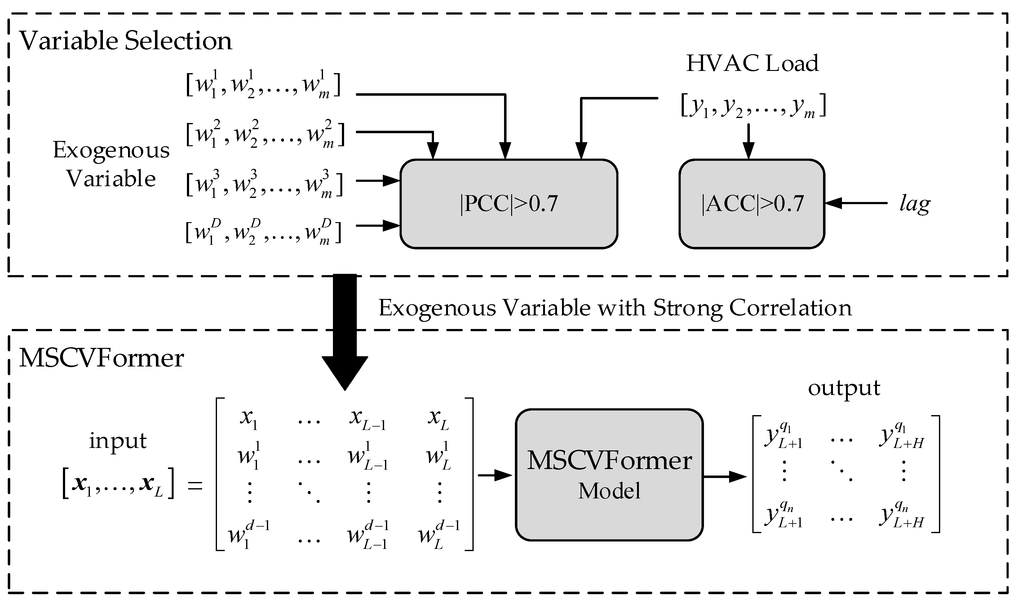
Figure 1. The data flow of HVAC load forecasting.
Energies 18 05073 g001
Figure 2. The flowchart of MSCVFormer.
Energies 18 05073 g002
Figure 3. The MSA mechanism.
Energies 18 05073 g003
Figure 4. The curve of the aggregated load in the WPuQ dataset.
Energies 18 05073 g004
Figure 5. The correlation coefficient in the WPuQ dataset.
Energies 18 05073 g005
Figure 6. The curve of the aggregated load in the EnergyDetective2020 dataset.
Energies 18 05073 g006
Figure 7. The correlation coefficient in the EnergyDetective2020 dataset.
Energies 18 05073 g007
Figure 8. The MAPE of different steps: (ad) represent the results in various cases of the WPuQ dataset.
Energies 18 05073 g008
Figure 9. The PICP of probabilistic load forecasting for different confidence levels: (ad) represent the results in various cases of the WPuQ dataset.
Energies 18 05073 g009
Figure 10. The probabilistic forecasting of the proposed method in each case: (ad) represent the results in various cases of the WPuQ dataset.
Energies 18 05073 g010
Table 1. The time range of the four cases.
Training SetValidation SetTest Set
WPuQCase 11 January 2019–30 November 20191 December 2019–31 December 20191 January 2020–31 March 2020
Case 21 April 2019–29 February 20201 March 2020–31 March 20201 April 2020–30 June 2020
Case 31 July 2019–31 May 20201 June 2020–30 June 20201 July 2020–30 September 2020
Case 41 October 2019–31 August 20201 September 2020–30 September 20201 October 2020–31 December 2020
EnergyDetective2020Case 11 January 2015–30 November 20151 December 2015–31 December 20151 January 2016–31 March 2016
Case 21 April 2015–29 February 20161 March 2016–31 March 20161 April 2016–30 June 2016
Case 31 July 2015–31 May 20161 June 2016–30 June 20161 July 2016–30 September 2016
Case 41 October 2015–31 August 20161 September 2016–30 September 20161 October 2016–31 December 2016
Table 2. The hyperparameter sets of benchmarks.
ModelHyperparameter Settings
PM-
GBRWeak regressor = ‘Decision tree’, Estimators number = 20, Learning rate = 0.1, Max depth = 3
BiLSTMLSTM structure = [128, 128], Bidirectional = True
CNN-LSTMConv1d structure = [48,48], LSTM structure = [128,128], activation function= ReLU, learning rate = 2 × 10⁻⁴
TransformerConv1d structure = [48,48], Transformer structure = [128,128], activation function= ReLU, learning rate = 2 × 10⁻⁴
AutoformerConv1d structure = [48,48], Autocorrelation structure = [128,128], activation function= ReLU, learning rate = 2 × 10⁻⁴
Table 3. The structure of the proposed method.
LayerHyperparameters
InputHistorical load seriesHistorical temperature series
1Linear (1, 128)Linear (1, 128)
2Conv1d (48, 48)Conv1d (48, 48)
3Position encodingPosition encoding
4MSA BlockMSA Block
5CVA Block-
6[Fully connected layer (48 × 128, 24)] × 19-
Output 24 h multi-horizon quantile prediction result-
Table 4. The deterministic forecasting results of the proposed method on varying datasets.
MethodCase1Case2Case3Case4
RMSEMAPERMSEMAPERMSEMAPERMSEMAPE
WPuQPM5.3719.663.3245.161.8949.164.3121.38
GBR4.1619.142.0867.911.4976.923.2818.46
BiLSTM4.1218.221.6740.801.4340.153.4019.75
CNN-LSTM3.7917.171.4936.671.1937.053.2018.15
Transformer3.6015.601.4535.281.2332.043.1918.37
Autoformer3.6315.741.4432.681.2435.083.2119.23
MSCVFormer3.5415.031.4631.961.2333.413.0917.09
Energy
Detective
2020
PM463.5859.80325.8166.65785.3255.91287.9652.36
GBR455.4355.36301.2560.83733.6248.41256.9446.23
BiLSTM423.7647.13287.6540.76611.8939.43213.4638.77
CNN-LSTM412.6134.17240.3332.46546.0634.57204.7627.82
Transformer216.6818.29186.7322.95294.2823.56145.6319.43
Autoformer172.6317.22188.5423.55301.4622.97137.8518.55
MSCVFormer156.2815.66165.2820.22248.5621.14120.2817.79
Table 5. The probabilistic forecasting results of the proposed method on varying datasets.
MethodCase1Case2Case3Case4
PICPPINAWPICPPINAWPICPPINAWPICPPINAW
WPuQGBR0.9590.5050.7730.6990.8521.0890.9750.596
BiLSTM0.9050.3680.8000.3430.8720.3630.9230.395
CNN-LSTM0.8930.3190.8040.2880.8360.3020.9150.352
Transformer0.9070.3080.8250.2640.9140.3190.8940.330
Autoformer0.8800.3540.8470.2250.9040.3300.8800.274
MSCVFormer0.8770.2790.8900.2920.9060.2900.8970.296
Energy
Detective
2020
GBR0.9370.4080.9440.5480.8530.6450.9220.421
BiLSTM0.8980.2890.8800.2200.8690.2420.8720.210
CNN-LSTM0.9310.2420.8780.1570.8730.2320.8710.180
Transformer0.8590.0670.8070.0610.8390.0780.8170.073
Autoformer0.8890.1680.8500.1190.8800.2030.9180.214
MSCVFormer0.8940.0650.8810.0650.8750.0980.8730.081
Disclaimer/Publisher’s Note: The statements, opinions and data contained in all publications are solely those of the individual author(s) and contributor(s) and not of MDPI and/or the editor(s). MDPI and/or the editor(s) disclaim responsibility for any injury to people or property resulting from any ideas, methods, instructions or products referred to in the content.