Article

Short-Term Load Forecasting in the Greek Power Distribution System: A Comparative Study of Gradient Boosting and Deep Learning Models

by
Md Fazle Hasan Shiblee
and
Paraskevas Koukaras
*
School of Science and Technology, International Hellenic University, 14th km Thessaloniki-Moudania, 57001 Thessaloniki, Greece
*
Author to whom correspondence should be addressed.
Energies 2025, 18(19), 5060; https://doi.org/10.3390/en18195060
Submission received: 27 August 2025 / Revised: 11 September 2025 / Accepted: 20 September 2025 / Published: 23 September 2025

Abstract

Accurate short-term electricity load forecasting is essential for efficient energy management, grid reliability, and cost optimization. This study presents a comprehensive comparison of five supervised learning models—Convolutional Neural Network (CNN), Long Short-Term Memory (LSTM), Gated Recurrent Unit (GRU), a hybrid (CNN-LSTM) architecture, and Light Gradient Boosting Machine (LightGBM)—using multivariate data from the Greek electricity market between 2015 and 2024. The dataset incorporates hourly load, temperature, humidity, and holiday indicators. Extensive preprocessing was applied, including K-Nearest Neighbor (KNN) imputation, time-based feature extraction, and normalization. Models were trained using a 70:20:10 train–validation–test split and evaluated with standard performance metrics: MAE, MSE, RMSE, NRMSE, MAPE, and R 2 . The experimental findings show that LightGBM beat deep learning (DL) models on all evaluation metrics and had the best MAE (69.12 MW), RMSE (101.67 MW), and MAPE (1.20%) and the highest R 2 (0.9942) for the test set. It also outperformed models in the literature and operational forecasts conducted in the real world by ENTSO-E. Though LSTM performed well, particularly in long-term dependency capturing, it performed a bit worse in high-variance periods. CNN, GRU, and hybrid models demonstrated moderate results, but they tended to underfit or overfit in some circumstances. These findings highlight the efficacy of LightGBM in structured time-series forecasting tasks, offering a scalable and interpretable alternative to DL models. This study supports its potential for real-world deployment in smart/distribution grid applications and provides valuable insights into the trade-offs between accuracy, complexity, and generalization in load forecasting models.

1. Introduction

1.1. Motivation and Incitement

Short-term load forecasting (STLF) is a crucial process in the efficient and reliable operation of modern power systems. It enables grid operators to optimize electricity production, ensure grid stability, and reduce operational costs. STLF focuses on predicting electricity demand over short horizons, typically from a few minutes to a few days, and has a direct impact on energy management, scheduling, and pricing strategies, especially in situations of fluctuating and unpredictable demand [1,2].
The increasing integration of renewable energy sources such as solar and wind has made STLF even more challenging as these sources are inherently intermittent and weather-dependent. Traditional linear forecasting models, such as Autoregressive Integrated Moving Average (ARIMA), often fail to capture the non-linear relationships and highly dynamic consumption patterns caused by sudden weather fluctuations, consumer behavior changes, and economic variations [3,4].
This shift in energy consumption behavior has driven the transition toward machine learning (ML) and deep learning (DL) techniques, which are capable of handling complex, non-linear, and temporal dependencies. Among these, Long Short-Term Memory (LSTM) networks have shown great potential in STLF due to their ability to model long-term dependencies and handle volatile time-series data effectively [5]. LSTMs are increasingly being combined with Convolutional Neural Networks (CNNs) to exploit both temporal and spatial features, improving forecasting performance by automating feature extraction [2].

1.2. Literature Review and Research Gaps

In recent years, several studies have applied ML, DL, and hybrid approaches to improve STLF accuracy, particularly for the Greek power system, where seasonal variability and demand fluctuations pose significant challenges.
The authors of [1] investigated STLF for the building sector using models such as HGBR and LGBMR, showing that feature engineering and the choice of time resolutions significantly affect forecasting accuracy and computational performance. Similarly, the authors of [6] proposed transforming high-dimensional hourly load data into a univariate series using Singular Value Decomposition (SVD), followed by ARIMA, which explained 91% of the variance and simplified the problem.
Another work [7] improved STLF accuracy by applying Artificial Neural Networks (ANNs) with inputs from previous day (D-1) and weekly (D-7) load patterns combined with temperature, achieving a MAPE of 1.92%, one of the lowest errors reported in Greek forecasting. A hybrid approach was introduced in [8], combining fuzzy clustering, RBFNNs, and CNNs, achieving superior accuracy for both the Greek interconnected system and the isolated Crete network. Similarly, Ref. [9] used Feed-Forward ANNs (FF ANN), achieving a MAPE of 3.66%, and highlighted that input data quality plays a critical role in achieving accurate predictions.
Other studies have focused on hybrid models and time-series decomposition techniques. Ref. [10] combined Singular Spectrum Analysis (SSA) with LSTM networks, effectively capturing complex seasonalities and improving prediction performance. Likewise, Ref. [11] introduced the Dynamic Block-Diagonal Fuzzy Electric Load Forecaster (DBD-FELF), which integrates fuzzy clustering with RNNs, achieving a MAPE of 1.18% while maintaining lower computational complexity than many DL models.
DL has also been combined with chaos theory to improve STLF accuracy. Ref. [12] used RNNs, GRUs, LSTMs, and Bi-LSTMs for iterative predictions and found GRUs particularly robust under chaotic load conditions. Meanwhile, Ref. [13] applied Transfer Learning (TL) with clustering techniques to improve day-ahead forecasting across several European countries, including Greece, showing that knowledge transfer between regions with similar consumption patterns enhances prediction performance.
Finally, Ref. [14] developed a hybrid clustering–neural network model for bus-level forecasting, demonstrating improved prediction reliability during peak demand periods.

1.3. Identified Gaps

Despite these advances, several key challenges remain:
  • Studies using the ENTSO-E hourly load dataset for Greece often report relatively high forecasting errors, showing the difficulty of accurately predicting national-level demand.
  • Existing DL-based approaches provide high accuracy but are often computationally expensive and lack interpretability.
  • Many studies focus on single-model forecasting, whereas hybrid and ensemble approaches could better handle diverse demand patterns.
  • The use of real-time IoT and smart meter data in STLF remains underexplored, limiting adaptability in dynamic grid environments.
These gaps highlight the need for comprehensive comparative studies using state-of-the-art ML and DL models on large, realistic multivariate datasets to improve STLF performance.

1.4. Novelty, Contributions, and Paper Organization

This study addresses the above gaps by evaluating five state-of-the-art forecasting models on a multivariate dataset for the Greek power system covering 2015–2024. The dataset includes hourly electricity load, weather variables (temperature, humidity), and holiday indicators, providing a realistic context for testing model performance.
The main contributions of this paper are as follows:
  • Comprehensive Model Evaluation: Benchmarking and comparing LightGBM, LSTM, GRU, CNN, and CNN-LSTM hybrid models for short-term load forecasting on a real-world Greek dataset.
  • Realistic and Extensive Dataset: Using a multivariate dataset spanning nine years, enabling testing under realistic operational conditions.
  • Advanced Data Preprocessing: Implementing KNN imputation, feature engineering, and data normalization to improve prediction quality.
  • Evaluation with Multiple Metrics: Assessing models using MAE, RMSE, MAPE, R 2 , and NRMSE, providing a comprehensive evaluation framework.
  • Addressing Forecasting Challenges: Tackling common STLF issues such as overfitting, computational resource limitations, and hyperparameter optimization to ensure model robustness.
  • Explicit trade-off analysis: We quantify and discuss the trade-offs between accuracy, model complexity, and generalization across DL architectures and LightGBM, providing actionable guidance for model selection under real-world constraints.
Finally, the rest of this paper is organized as follows. Section 2 describes the dataset, its sources, and the preprocessing techniques applied to ensure data quality and consistency. Section 3 presents the machine learning and deep learning models used in this study, along with the training procedures and evaluation methodology. Section 4 reports the experimental findings, compares the performance of the models, and discusses their implications for practical deployment. Lastly, Section 5 summarizes the main contributions of this work and provides recommendations for future research directions.

2. Data Curation and Analysis

This section covers three broad areas: data collection, data processing, and feature selection. The first subsection provides a description of the dataset, its source, and major features. The second subsection explains the data processing methods employed to prepare the data for ML and DL analysis. Understanding these aspects and applying them appropriately is essential when working with datasets in predictive modeling.

2.1. Dataset Description

The data used in this research is based on the Greek Electricity Distribution and Management System, specifically the hourly actual load data. This information was obtained from the European Network of Transmission System Operators for Electricity (ENTSO-E) (https://transparency.entsoe.eu/) (accessed on 10 July 2025). The dataset is organized as a single time series, where each entry represents the actual electricity load in megawatt-hours (MWh) for a specific hour and date. This time-series structure reflects the consumption dynamics of the Greek electricity system and provides a solid foundation for short-term load forecasting [6,7,9].
To enhance the predictive power of the model, additional variables were included due to their influence on electricity demand. Hourly temperature and humidity data for the period 2015–2024 were retrieved using the Python Meteostat API (https://pypi.org/project/meteostat/) (accessed on 10 July 2025). Given the challenge of accounting for weather variations across the entire country, weather data from Athens—one of Greece’s major urban centers—was used to represent national trends, thereby simplifying the model while maintaining relevance. Athens weather data were used because it represents the largest load center in Greece and strongly influences national demand. This choice captured the main seasonal and peak variations that drive overall load trends while acknowledging possible bias during regionally heterogeneous weather and leaving multi-station/reanalysis inputs for enhancing the robustness of future work. Furthermore, public holidays were considered by retrieving holiday indicators using the Python holidays API (https://pypi.org/project/holidays/) (accessed on 10 July 2025). These indicators helped capture anomalies in demand during non-working days.
For model training, the dataset was split chronologically. Data from 2015 to 2021 was used for training, 2022 and 2023 data was used for validation, and 2024 data was used as a test set. This setup allowed the models to learn from historical patterns, tune hyperparameters based on recent data, and be evaluated on completely unseen data. This strategy ensured generalizability and provided a realistic assessment of model performance in forecasting future electricity demand.

2.2. Data Preprocessing and Feature Engineering

After initial data cleaning, several preprocessing steps were applied to prepare the dataset for modeling. Feature engineering was first performed to extract time-dependent patterns from the raw data [15]. Temporal features such as hour, day, weekday, month, and year were derived from the timestamp to capture daily, weekly, and annual seasonality. Additionally, lag-based features were introduced to incorporate historical load information, including
  • lag_1: Load at the previous hour;
  • lag_24: Load at the same hour on the previous day;
  • lag_168: Load at the same hour on the previous week.
Rolling averages were also computed to reflect short-term trends:
  • rolling_mean_3: 3 h moving average;
  • rolling_mean_24: 24 h moving average.
To handle missing values, K-Nearest Neighbor (KNN) imputation was used. KNN is well-suited for time-series data with recurrent patterns as it imputes values based on the similarity to neighboring observations, thereby preserving the inherent structure of the dataset [16].
After feature generation and imputation, the dataset was normalized to have zero mean and unit variance. This step ensured that all features contributed equally to model training and helped stabilize the learning process for many ML algorithms.
Finally, the dataset was split into training, validation, and testing subsets using a 70:20:10 ratio. The training set (2015–2021) was used to train the models, the validation set (2022–2023) to fine-tune hyperparameters, and the test set (2024) to evaluate final performance. Stratified partitioning was employed to ensure even distribution of load patterns and maintain the seasonal and temporal structure across splits. This robust preprocessing pipeline enhanced data quality and ensured that the resulting models were capable of producing reliable and accurate short-term load forecasts [17].

2.3. Feature Importance Analysis

Figure 1 illustrates the feature importance as determined by the LightGBM model applied to the short-term load forecasting (STLF) task. The most significant predictor was the hour, highlighting the strong influence of time of day on electricity consumption. Historical features like lag_1 (previous hour) and lag_24 (previous day) also ranked highly, confirming the importance of recent past data in load prediction.
The rolling_mean_3 feature, representing a 3 h smoothed trend, indicated the model’s reliance on short-term moving averages to detect consumption patterns. Temperature was also among the top contributors, suggesting that weather has a considerable effect on electricity usage.
Other influential features included lag_168 (weekly lag), month, and weekday, which incorporated seasonal and weekly patterns. Conversely, variables such as year, day, humidity, and is_holiday showed lower importance. This implied that long-term trends and humidity played a smaller role and that public holidays had a limited influence in this context.
Overall, the feature importance analysis suggested that temporal variables and temperature are the most impactful for short-term load forecasting, while calendar-specific factors are relatively minor in predictive power.

3. Model Architectures and Experimental Setup

The section outlines the baseline models employed in this study, along with the experimental setup and the model training process. It provides a detailed description of the various models used for comparison and the steps taken to train and evaluate them, ensuring a comprehensive understanding of the approach adopted for short-term load forecasting.

3.1. CNN (Convolutional Neural Network)

CNNs have been most successful in image processing; however, they have also found application in time-series forecasting, such as short-term load forecasting. CNNs use convolutional layers to process the input data, where a filter is applied to scan the data and assist in locating local patterns in the data. CNNs are used in the short-term load forecasting context by identifying local load changes, including sudden changes and periodic increases or decreases, which frequently take place because of such factors as weather changes, holidays, or sudden changes in consumption patterns. Such local patterns are vital in short-term forecasting, where rapid adjustments should be made depending on recent variations in load. CNNs are good at detecting these patterns and are able to handle large quantities of data. They are able to automatically learn and extract features of raw data, so there is no need for manual feature engineering. CNNs are specifically well-suited to cases in which recent data or small time windows are the most predictive of future consumption patterns [18,19].

3.2. LSTM (Long Short-Term Memory)

LSTM networks are a variant of Recurrent Neural Networks (RNNs) that are specifically developed to learn long-term dependencies in sequential data. In contrast to the traditional RNNs, LSTMs have special memory cells and gates (input, forget, and output gates), which enable them to remember information across long time series, and, thus, they are very useful in time-series applications like short-term load forecasting. LSTMs are particularly effective in this field at capturing complicated temporal dependencies where the past energy consumption affects the future demand. As an example, LSTMs are able to learn seasonal patterns, daily load patterns, and other periodic patterns that influence energy consumption. The capability of LSTMs to store information over a long time is useful in predicting energy loads that are based on other factors, like the consumption of the previous day or even longer-term trends. This capability to capture both long-term dependencies (such as daily, weekly, and yearly trends) and short-term variability is the reason why LSTMs are one of the most popular models to forecast time series, including energy load forecasting [18,20].

3.3. Hybrid Model (CNN-LSTM)

The hybrid (CNN-LSTM) model integrates the strengths of both CNN and LSTM networks, enabling the capture of local as well as long-term dependencies in time series data. The CNN layers are employed to extract local features or patterns in the energy consumption data by filtering the input sequence, with particular attention to short-term variations such as sudden spikes or sharp drops in load. In contrast, the LSTM layers are designed to model long-term dependencies and trends, including seasonal patterns, which occur over extended periods. This hybrid approach leverages the complementary capabilities of the two architectures: CNNs are effective for feature extraction, while LSTMs are well suited for modeling temporal dependencies. Consequently, the model is particularly advantageous for forecasting energy loads, where both short-term fluctuations and long-term regularities play a crucial role. For instance, the CNN component may capture sudden variations in load caused by weather or special events, whereas the LSTM component can model recurring patterns such as the time of day or day of the week [21].
In this study, the hybrid CNN-LSTM model was implemented using two convolutional layers (128 and 64 filters with kernel sizes of 5 and 3, respectively), followed by max pooling and dropout to ensure robust feature extraction. The output was then processed by two stacked LSTM layers (128 and 64 units), allowing the model to capture sequential dynamics. Finally, dense layers with 64 and 32 neurons were used to generate the regression output. The training process utilized the Adam optimizer with a learning rate of 0.0001, the mean squared error (MSE) as the loss function, and a batch size of 32. To improve generalization and prevent overfitting, callbacks such as early stopping and learning rate scheduling were incorporated.

3.4. GRU (Gated Recurrent Unit)

GRUs are another variant of Recurrent Neural Networks (RNNs) that, like LSTMs, are designed to capture sequential dependencies in time-series data. Nevertheless, GRUs have fewer parameters and are computationally less expensive than LSTMs. They possess fewer parameters since they do not need a dedicated memory cell like LSTMs and are thus easier to train and less likely to overfit. GRUs have two gates, reset and update gates, which determine the flow of information and what information to keep or forget. GRUs are effective in short-term load forecasting because they can model temporal dependencies in energy consumption, even when the available computational resources or training time are limited. GRUs are able to capture energy consumption trends, cycles, and fluctuations, even though they have a simpler architecture. They can be used as an alternative to LSTMs, particularly when the training is required to be faster and the number of parameters is reduced, without affecting the quality of the predictions [22].

3.5. LightGBM (Light Gradient Boosting Machine)

LightGBM is a very efficient and scalable gradient boosting framework that has been applied extensively to many ML applications, such as time-series forecasting, including short-term load forecasting. In contrast to traditional gradient boosting algorithms, LightGBM resorts to a histogram-based approach to the selection of the best splits, which makes it faster and memory-efficient. This is especially beneficial in cases where one has to deal with large datasets or where one requires rapid training of models. LightGBM works by constructing an ensemble of decision trees, each of which is trained to fix the mistakes of the preceding trees, in the case of short-term load forecasting. These trees are able to capture the non-linear relationships and interactions within the data, and, therefore, the model is very effective in predicting energy demand, which can be affected by a number of complex factors like weather conditions, time of day, and holidays. LightGBM is categorical variable-friendly and can use parallel and GPU learning, making it scale well on larger datasets. LightGBM has been a very good option in forecasting applications where speed and accuracy are of the essence due to its ability to model non-linear relationships and work with large amounts of data [23].

3.6. Experimental Setup and Model Training

In order to compare the performance of the various learning paradigms in short-term electricity load forecasting, five advanced models were designed and trained, each with unique architectural merits. The DL architectures were LSTM, CNN, the combination of CNN and LSTM, and GRU networks. The LSTM model (a variant of the Recurrent Neural Network (RNN)) was selected because it can model long-range temporal dependencies that exist in sequential data. The CNN, which is normally applied to spatial data, was modified to time-series forecasting by taking advantage of one-dimensional convolutional layers to learn local temporal features in an efficient manner. The CNN-LSTM hybrid model took the best of both models, where CNN layers were employed first to capture short-term patterns, after which LSTM layers that captured sequential dependencies were applied. GRU, a variant of LSTM that has a simpler gating structure and fewer parameters, was found to perform similarly with lower computational complexity.
Along with the DL architectures, a tree-based ensemble model, Light Gradient Boosting Machine (LightGBM), was used. LightGBM is a fast, scalable, and efficient gradient boosting framework that is particularly fast and scalable and works well with tabular data. It is not explicitly temporal-modeling but rather learns using a rich set of engineered features such as lag values, rolling statistics, calendar-based variables, and weather-related inputs. We used LightGBM as the boosted-tree baseline (chosen over XGBoost for faster, more memory-efficient training at our scale) and omitted models like ARIMA and SVR due to poor scalability to long, multivariate hourly series, which made them impractical for our 10-year dataset. Every DL model was trained on TensorFlow/Keras and LightGBM was trained on its own Python library. The hyperparameters of all models were fine-tuned by grid search and monitoring of validation to maximize forecasting performance.
The MSE loss function was used to train the model, and the training and validation sets were used to inform the learning process and avoid overfitting. A number of callbacks were introduced in the training to enhance model generalization. Early stopping was used to terminate the training process when validation loss failed to decrease in 20 consecutive epochs, thereby avoiding unnecessary computations and overfitting. The model weights were saved at the best-performing validation epoch using a model checkpoint mechanism. Furthermore, the ReduceLROnPlateau callback was applied to dynamically change the learning rate in case of stagnation of the validation loss, which made convergence more precise.
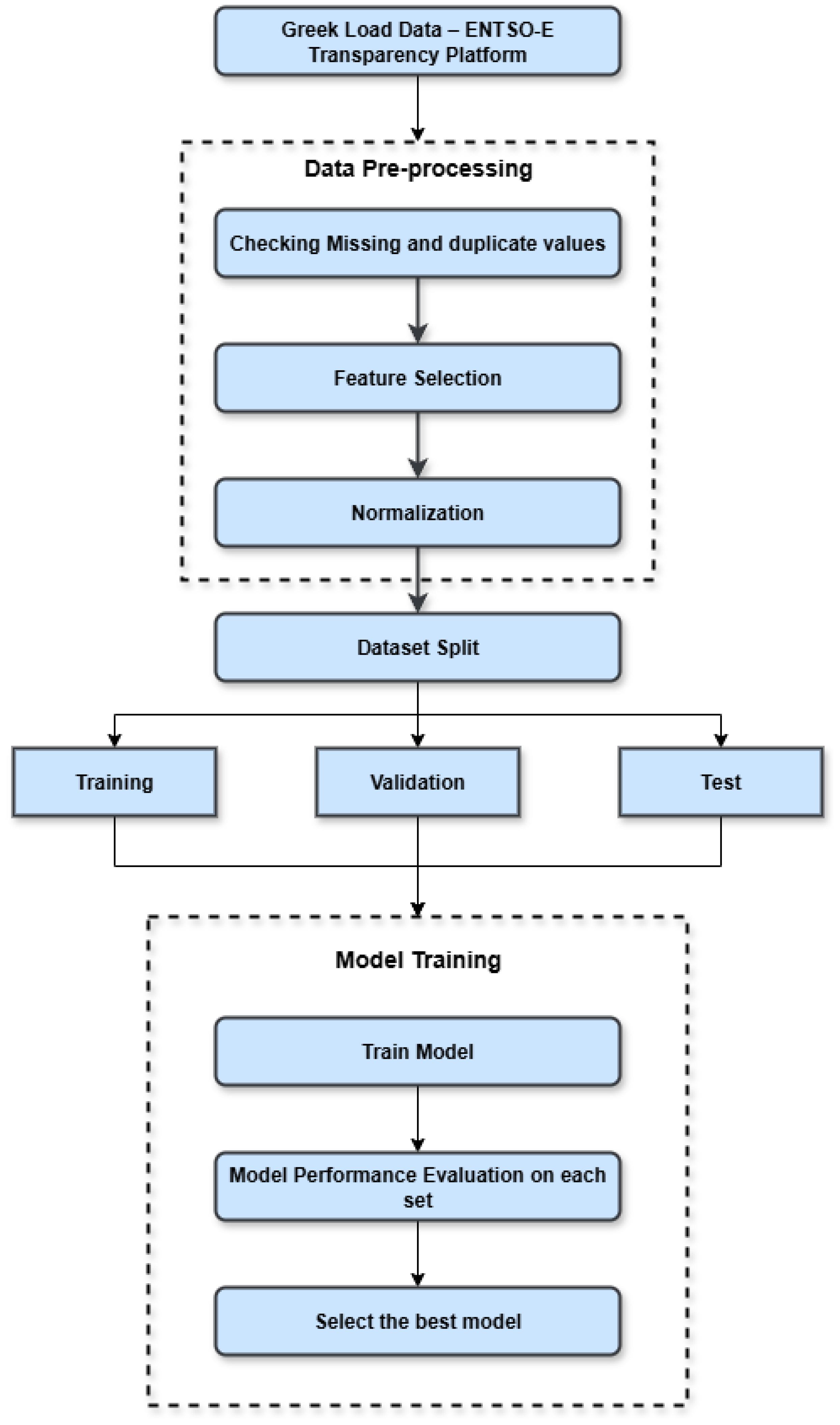
The performance was evaluated based on five statistical measures, which included MAE, RMSE, MAPE, R 2 score, and NRMSE. These measures were calculated on the validation and test sets to evaluate the accuracy and generalization ability of each of the models. Notably, the 2024 test set was not used in any way during training or validation to give an objective indication of out-of-sample predictive performance. The LightGBM model was the best-performing model in all the metrics, with a low error rate and a high R 2 score compared to the DL models. The fact that it could deal with heterogeneous feature types and optimize the gradient boosting effectively made it especially useful in this forecasting task. The general process of the experiment, data preprocessing, data splitting, model training, model evaluation, and model selection are depicted in Figure 2.
Aside from predictive performance, we also contrasted the computational footprint of each model. In our setting, the sequence models (LSTM, GRU) and the CNN-LSTM hybrid had longer training and tuning cycles and more memory usage than tree-based boosting. CNN and GRU models trained more quickly than LSTM, but they had lower final accuracy. The CNN-LSTM hybrid added architectural complexity without corresponding benefits. LightGBM had lower training times and resource usage, corresponding to histogram-based learning and efficient tabular engineered feature handling. These differences informed the downstream assessment of scalability and real-time feasibility reported in Section 4.3.
Finally, to ensure comparability across architectures, all models were trained and evaluated on the same core variable set. This isolated modeling capacity from exogenous data availability and prevented twisting results due to heterogeneous feature sets.

4. Results and Discussion

This chapter includes the results of the test of the proposed short-term load forecasting models, which were used to predict the energy consumption of different datasets. To evaluate the performance of the models, a variety of evaluation metrics were used, which allowed us to compare them in detail with the existing approaches in load forecasting [24]. The findings indicate that the model developed using LightGBM consistently performed better than the other methods, which indicates its accuracy and reliability in short-term load prediction. Moreover, this section gives detailed explanations of all the evaluation metrics that were employed in the analysis in order to gain a thorough comprehension of the performance of the models.

4.1. Performance Evaluation Metrics

A number of metrics to quantify the performance of our approach in predicting electrical load, namely, MAE, RMSE, MSE, MAPE, NRMSE, and R 2 , were employed in this study. MAPE is a percentage version of where MAE, MSE, and RMSE merely indicate the numerical difference between actual and estimated load. It shows the relationship between the actual outcomes and the forecasts in a straight line. NRMSE is more effective in demonstrating the utility of RMSE by examining the extent to which data is dispersed. The combination of all these statistics allowed us to demonstrate the validity of the forecasting model and enabled comparisons with other methods [25,26].

4.1.1. Mean Absolute Error (MAE)

Regression tasks often use MAE to find the average difference between predicted and real values. MAE measures the average size of errors in load forecasting, without paying attention to their direction. It is found by averaging the absolute difference between what is predicted and what is actually observed in every sample (Equation (1)).
MAE = 1 n i = 1 n L i , actual L i , predicted

4.1.2. Root Mean Squared Error (RMSE)

RMSE is the square root of the average squared difference between the actual and predicted load values. RMSE gives greater importance to larger errors than MAE, so it is more likely to notice outliers and big mistakes in forecasting (Equation (2)).
RMSE = 1 n i = 1 n L i , actual L i , predicted 2

4.1.3. Mean Squared Error (MSE)

MSE finds the average squared difference between forecasted and actual amounts of load. It helps assess the accuracy of a forecast by focusing on bigger mistakes (Equation (3)).
MSE = 1 n i = 1 n L i , actual L i , predicted 2

4.1.4. Mean Absolute Percentage Error (MAPE)

MAPE is the average percentage difference between actual and estimated load, so it does not depend on scale and is easy to understand in percentages (Equation (4)).
MAPE = 100 % n i = 1 n L i , actual L i , predicted L i , actual

4.1.5. Normalized Root Mean Squared Error (NRMSE)

NRMSE normalizes RMSE by the range of actual load values, providing a relative measure of prediction error that accounts for the variability in the data. Lower NRMSE values indicate higher predictive accuracy (Equation (5)).
NRMSE = 1 n i = 1 n L i , actual L i , predicted L max L min 2
where L max and L min denote the maximum and minimum load values in a dataset.

4.1.6. Coefficient of Determination ( R 2 )

The coefficient of determination, R 2 , quantifies the proportion of variance in actual load values that is explained by a forecasting model. It ranges from 0 to 1, where 1 indicates perfect prediction and 0 indicates that the model does not explain any variance (Equation (6)).
R 2 = 1 i = 1 n L i , actual L i , predicted 2 i = 1 n L i , actual L ¯ actual 2
Here, L ¯ actual is the mean of actual load values.
In the above formulas, n is the total number of samples, L i , actual denotes the actual load at sample i, L i , predicted is the predicted load, and L max and L min represent the maximum and minimum loads in the dataset, respectively.

4.2. Prediction Results and Comparative Analysis

In the evaluation phase, five models—CNN, LightGBM, LSTM, CNN-LSTM (hybrid), and GRU—were assessed for their short-term load forecasting performance. Each model was trained and tested under consistent conditions to ensure a fair comparison. Performance evaluation was conducted using six standard metrics: MAE, MSE, RMSE, MAPE, NRMSE, and R 2 . These metrics were used to measure the accuracy of each model’s predictions and their alignment with actual values. The detailed results for all models across the selected metrics are presented in the following tables.
Table 1 presents the performance metrics of the CNN model. The model achieved a training MAE of 126.89 MW, a validation MAE of 154.07 MW, and a test MAE of 148.05 MW. The corresponding RMSE values were 176.79 MW, 206.68 MW, and 194.10 MW, indicating moderate variance in prediction errors. The R 2 score ranged from 0.9706 to 0.9789, showing a good fit but not optimal compared to other models. MAPE values remained between 2.2% and 2.8% and NRMSE hovered around 0.024 across all sets, highlighting the CNN’s consistent yet limited ability to capture fine-grained fluctuations in the load data.
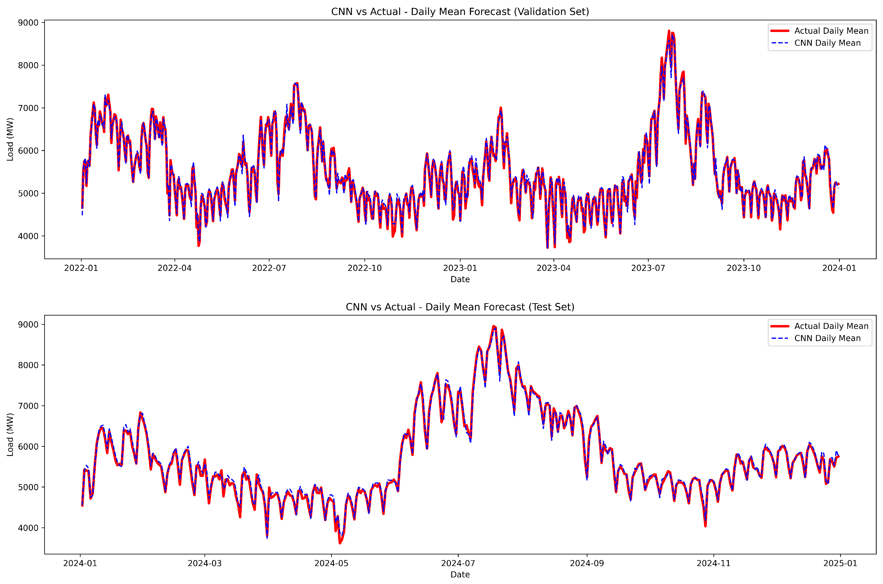
Figure 3 illustrates the comparison between actual and predicted daily mean electricity load values using the CNN model over the validation (top) and test (bottom) sets. The solid red line represents the actual daily mean load, while the dashed blue line indicates the CNN-predicted daily mean. The model successfully captured overall seasonal and daily consumption trends, closely following the fluctuations of real demand. While small deviations were observed during periods of abrupt load change (e.g., summer peaks), the model demonstrated strong alignment with the actual data, particularly during stable consumption periods.
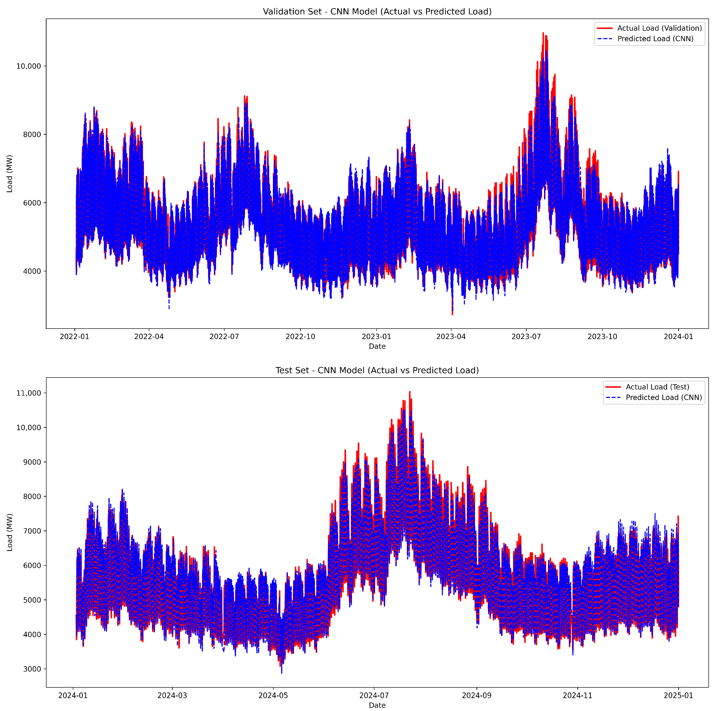
Figure 4 presents the hourly granularity forecast performance of the CNN model on the validation (top) and test (bottom) sets. The red line corresponds to the actual hourly load, while the blue dashed line shows the predicted load values. The model effectively tracked the short-term variability and high-frequency oscillations of electricity demand across nearly three years of data. The prediction accuracy was notably consistent during regular patterns but slightly less precise during high-volatility periods, such as summer peaks or holiday-related load shifts. These results indicate that the CNN model captures both periodic trends and local variations with reasonable fidelity.
Table 2 details the performance of the LSTM model, which significantly outperformed CNN and other DL architectures. The LSTM achieved lower error values across all metrics, with a test MAE of 87.26 MW, test RMSE of 118.68 MW, and notably high test R 2 score of 0.9921. The MAPE and NRMSE on the test set were 1.53% and 0.0149, respectively, suggesting strong accuracy and generalization capabilities. LSTM also maintained tight error bounds between training, validation, and test sets, indicating model robustness and minimal overfitting.
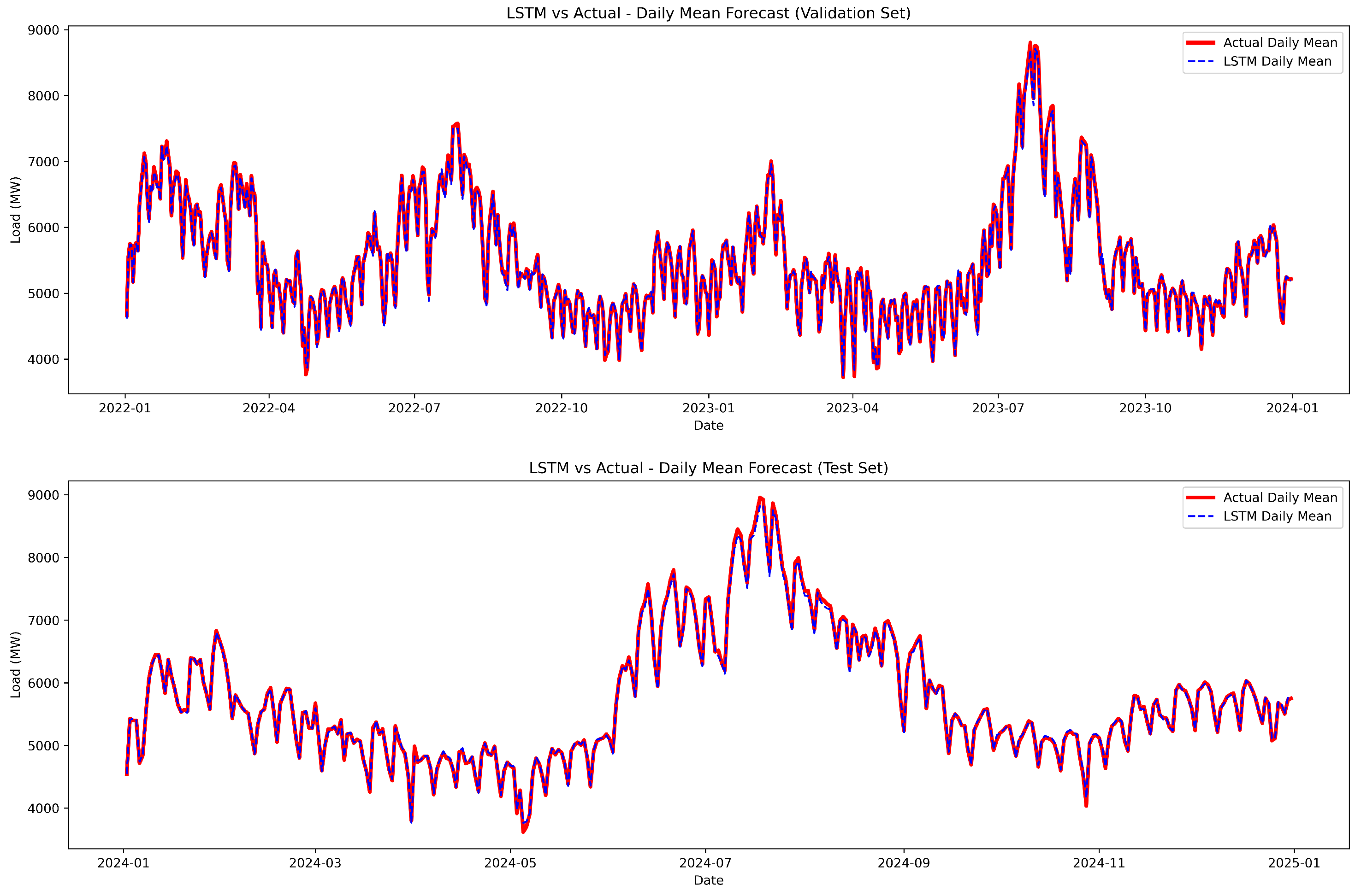
Figure 5 shows the comparison between the actual and predicted daily mean electricity load values generated by the LSTM model for the validation (top) and test (bottom) periods. The red line denotes the actual daily mean load, while the blue dashed line represents the LSTM forecast. The model tracked seasonal and intra-annual trends with high fidelity, especially during stable and moderately fluctuating load periods. Notably, the LSTM model demonstrated strong accuracy during high-demand months such as summer, with minimal lag or overshooting, confirming its strength in modeling long-term dependencies in sequential data.
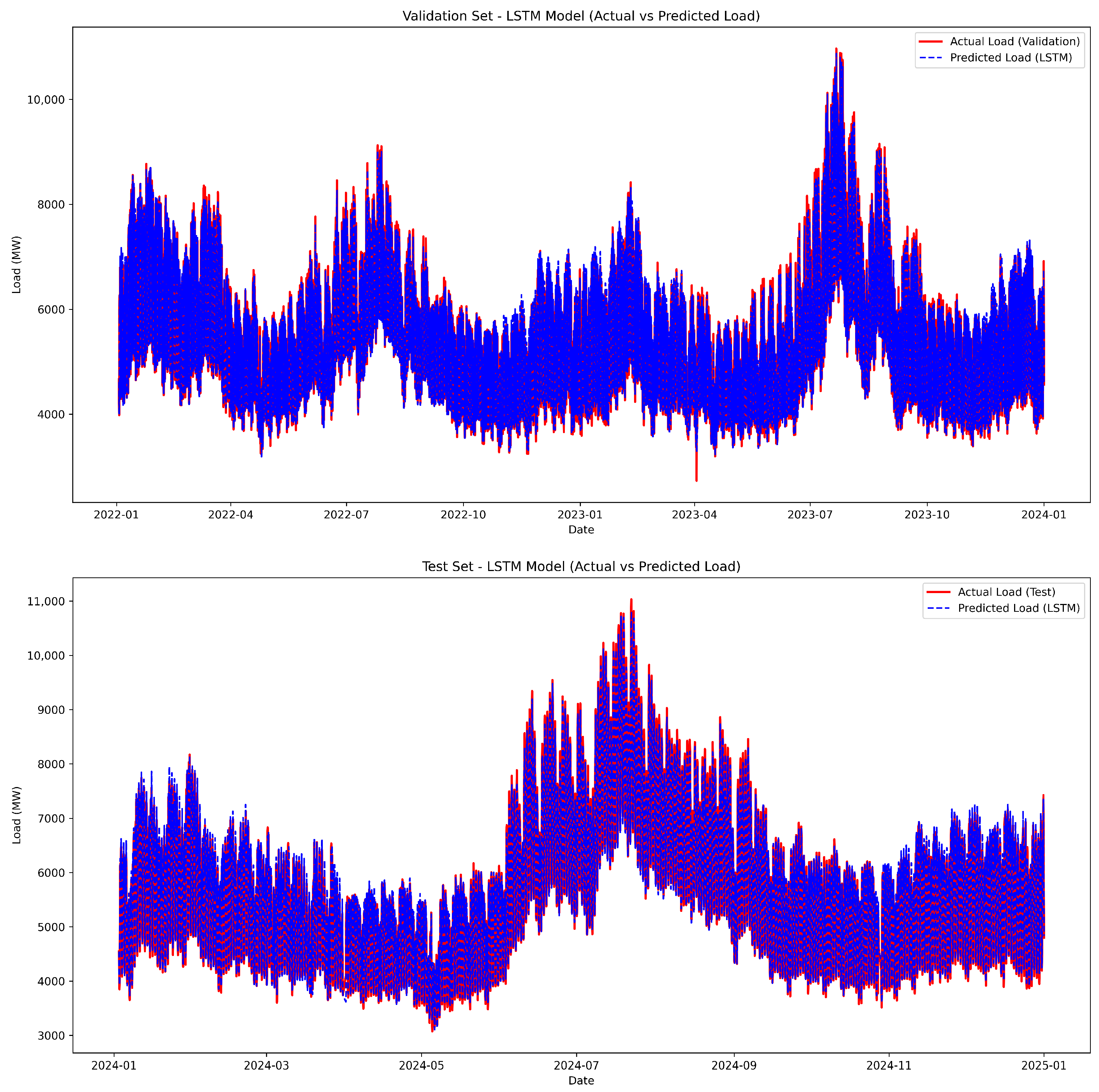
Figure 6 presents the detailed hourly forecasts of the LSTM model alongside the actual load for the validation set (top) and test set (bottom). The red curve represents the true hourly load, while the blue dashed line indicates the LSTM-predicted load. The model captured both high-frequency variations and broader seasonal patterns with considerable accuracy across the full time range. The overlap between the predicted and actual values demonstrates the LSTM model’s capacity to handle complex temporal dynamics in short-term load forecasting, with minimal prediction drift or phase mismatch.
Table 3 shows the metrics for the hybrid CNN-LSTM model. This combined architecture yielded a test MAE of 158.23 MW and a test RMSE of 258.05 MW, both higher than the individual CNN and LSTM models. Although the hybrid approach benefited from the CNN’s local pattern recognition and LSTM’s sequence modeling, the performance did not reflect synergy between the two. The R 2 score dropped to 0.9628 on the test set, with MAPE at 2.43% and NRMSE at 0.0324, confirming the hybrid model’s relatively lower predictive power in this context.
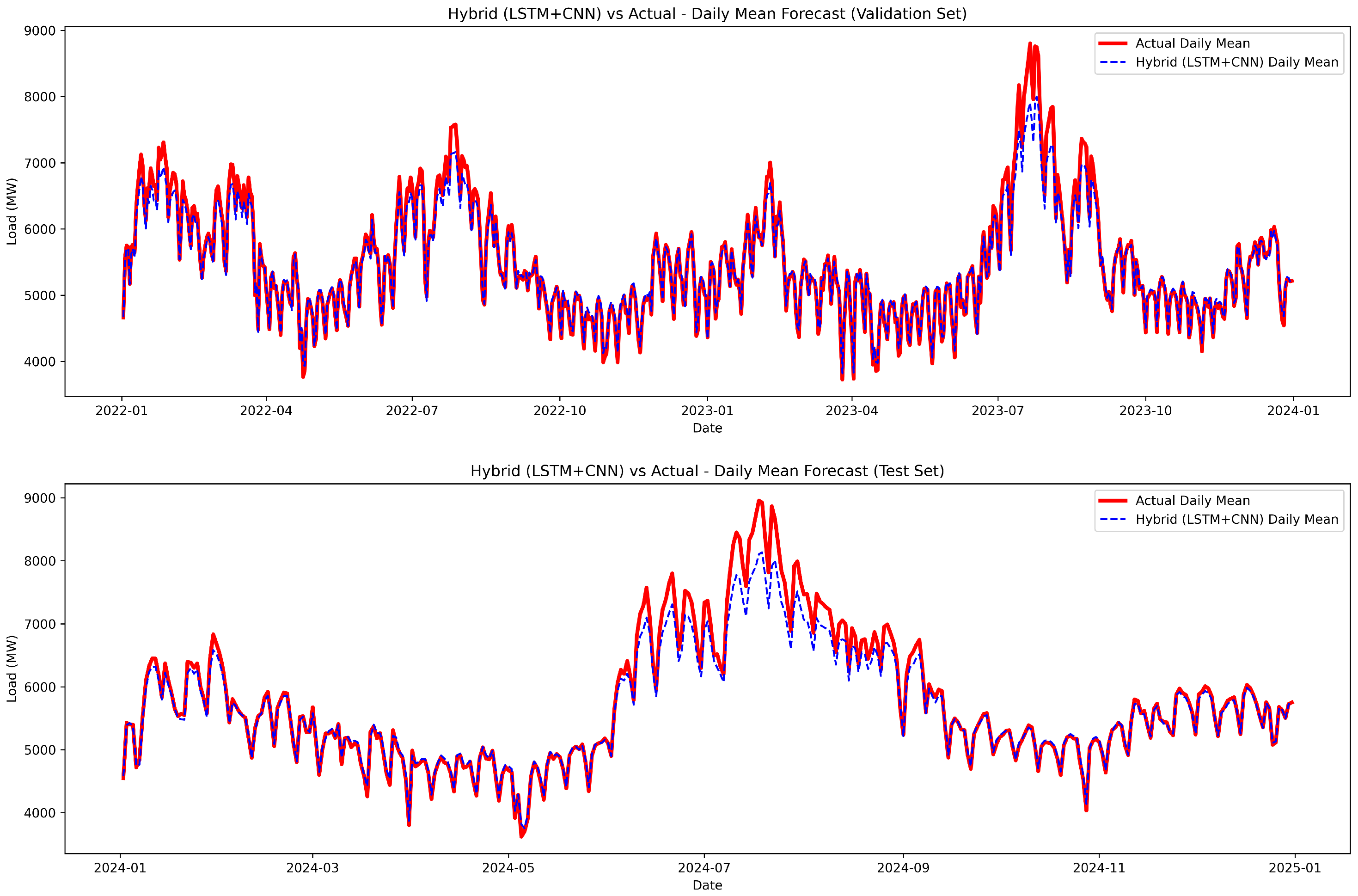
Figure 7 displays the comparison between the actual and predicted daily mean electricity load values generated by the hybrid CNN-LSTM model for both the validation (top) and test (bottom) sets. The red line represents the actual daily mean load, while the blue dashed line shows the hybrid model’s forecast. The model successfully captured overall load trends and seasonal shifts but exhibited noticeable underprediction during high-demand periods, especially in the summer months. This indicates that while the hybrid model effectively integrates spatial and temporal patterns, it may lack the responsiveness to sharp load peaks compared to other architectures.
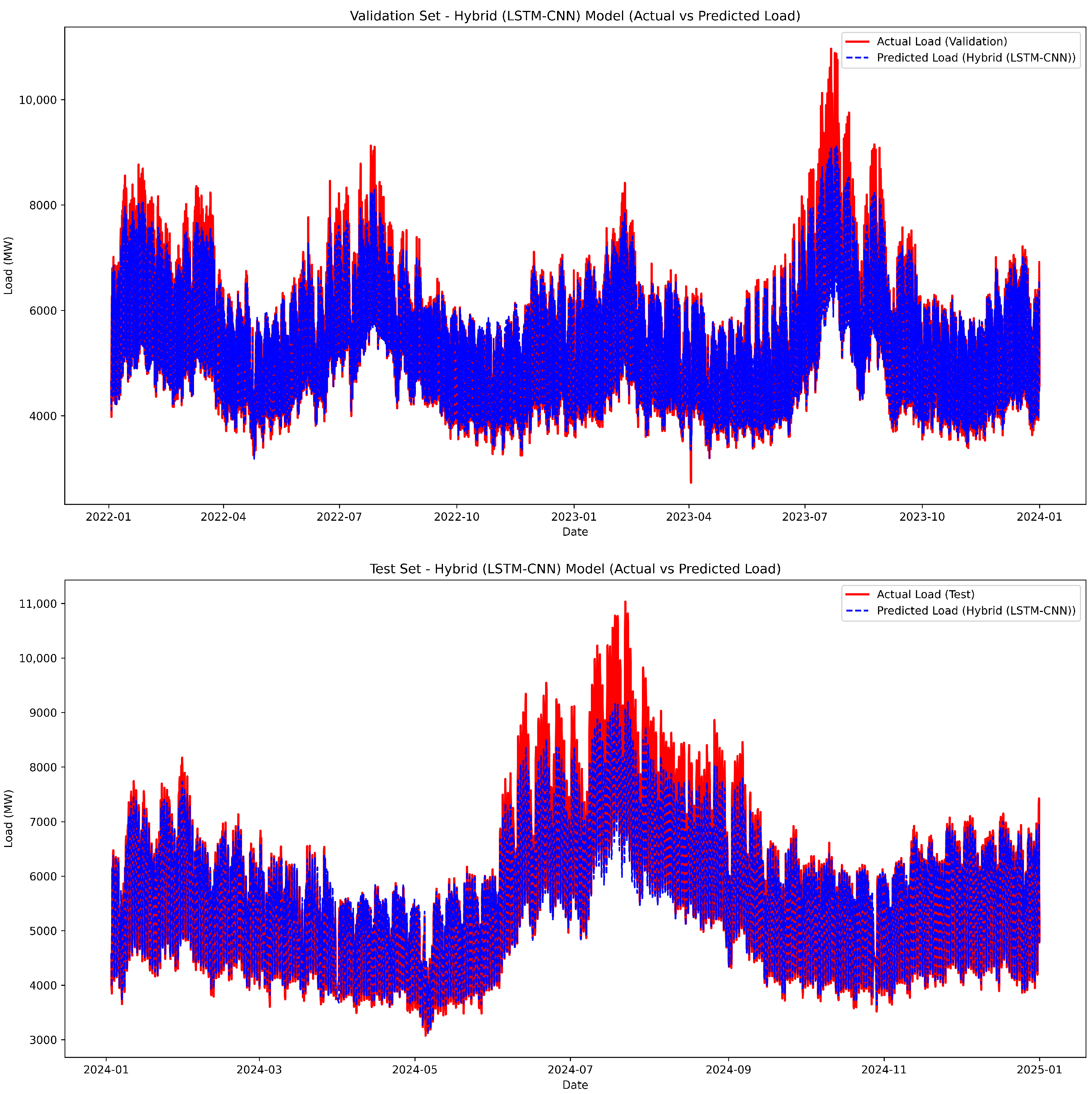
Figure 8 illustrates the hourly forecast performance of the hybrid CNN-LSTM model on the validation (top) and test (bottom) datasets. The actual load (red) and predicted values (blue dashed) are plotted to assess the model’s ability to capture short-term dynamics. While the model tracked the general structure of the load signal, discrepancies were evident during periods of high volatility, with significant underestimation during peak demand events. This suggests that the hybrid model may struggle to fully model high-amplitude, short-duration fluctuations despite leveraging both local pattern recognition (CNN) and long-term sequence modeling (LSTM).
Table 4 summarizes the GRU model’s performance. With a test MAE of 120.64 MW and RMSE of 158.80 MW, GRU performed better than the CNN and hybrid model but fell short of LSTM’s accuracy. The test R 2 score of 0.9859 and MAPE of 2.03% indicated strong, consistent performance, particularly considering GRU’s simplified architecture. GRU offers a balance between performance and training efficiency, making it a viable alternative when computational resources are constrained.
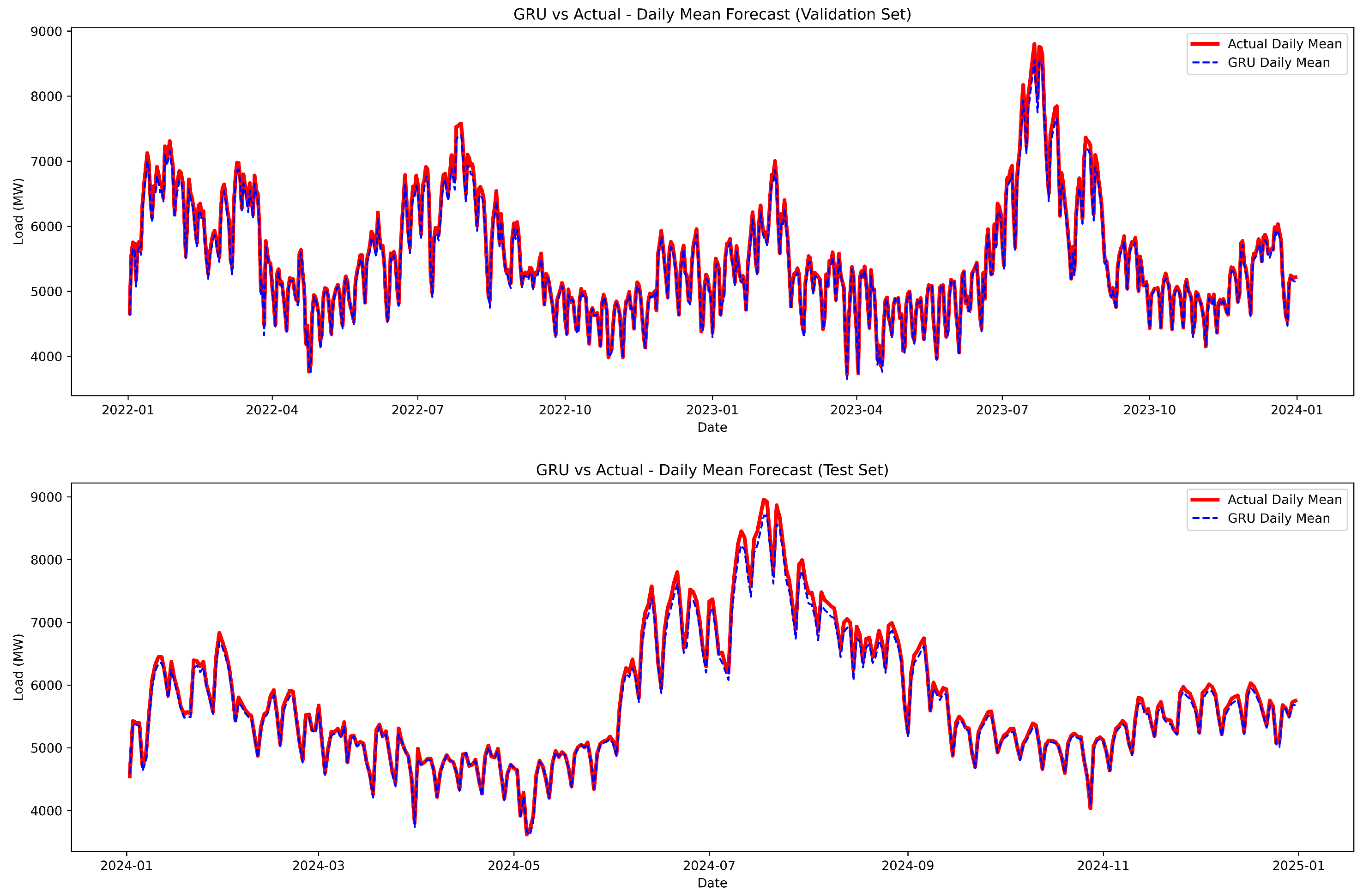
The performance of the GRU model in forecasting short-term electricity load is illustrated in Figure 9 and Figure 10.
As shown in Figure 9, which compares the actual and predicted daily mean load values, the GRU model demonstrated strong tracking of both seasonal and short-term consumption patterns across the validation and test sets. The predicted curves closely followed the actual values, with minimal lag or deviation, especially during periods of stable demand. However, there was a slight tendency to underpredict during peak summer months, though the model maintained overall high consistency and generalization. A more granular view of GRU’s performance is provided in Figure 10, which displays the hourly forecasts versus actual load for the same periods. The model accurately captured high-frequency variations and daily load cycles, including sharp increases and decreases in demand. While some underestimation was evident during extreme peak hours, the GRU model effectively maintained alignment with the ground truth across the entire timeline. This level of performance confirms the GRU’s capability to model complex sequential dependencies in load data while benefiting from a relatively simpler architecture compared to LSTM.
Table 5 presents the results of the LightGBM model, which outperformed all other architectures across every metric. The test MAE was only 69.12 MW, and the test RMSE was 101.66 MW—significantly lower than the rest. LightGBM also achieved the highest R 2 score of 0.9942 and the lowest MAPE and NRMSE values, at 1.20% and 0.0128, respectively. The consistent performance across train, validation, and test sets confirms its superior generalisation capability. LightGBM’s tabular feature learning, ability to handle non-sequential data, and computational efficiency give it a distinct advantage over DL models in this specific short-term load forecasting task.
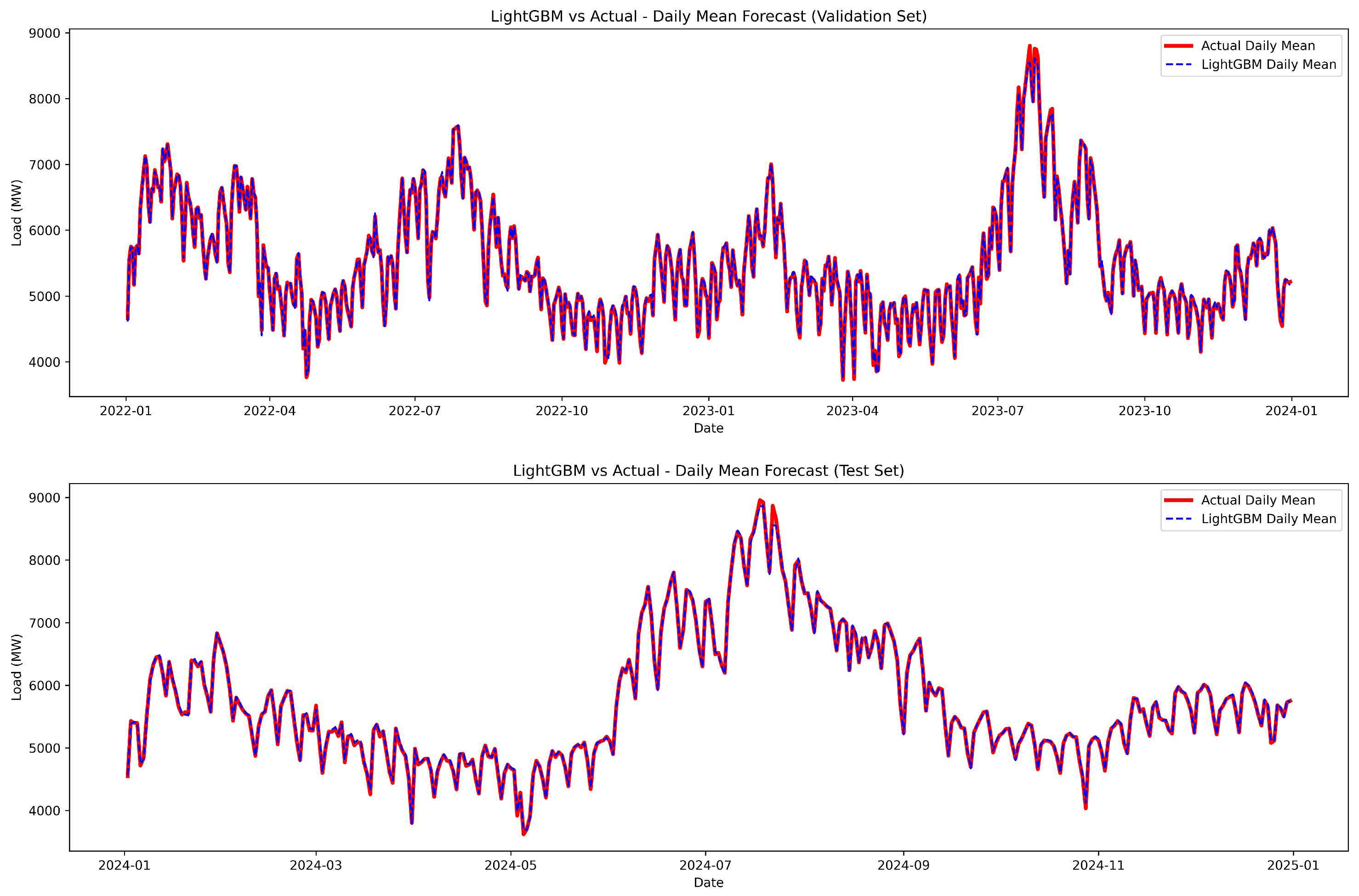
The forecasting performance of the LightGBM model, which outperformed all other tested architectures, is comprehensively illustrated in Figure 11 and Figure 12. As shown in Figure 11, the model’s predictions aligned almost perfectly with the actual daily mean load values across both validation (top) and test (bottom) sets. The red line represents the true daily mean load, while the blue dashed line indicates the LightGBM predictions. The nearly indistinguishable overlap of the two curves demonstrates the model’s ability to capture both short- and long-term patterns with exceptional precision. LightGBM effectively responded to seasonal fluctuations, daily demand cycles, and abrupt changes in consumption, including those occurring during high-load periods such as mid-summer.
In Figure 12, the model’s performance is examined at the hourly level. The red lines represent the actual hourly load for the validation (top) and test (bottom) periods, while the blue dashed lines denote the model’s predictions. Across both datasets, LightGBM showed remarkably accurate tracking of high-frequency load variations. Even during periods of extreme volatility, such as the peak summer months or the holiday season, the model closely followed the actual signal with minimal phase lag or amplitude mismatch. Importantly, the model maintained consistent performance across different seasons and demand regimes, reflecting strong generalization and robustness. This high level of accuracy confirms LightGBM’s capability to leverage feature-engineered inputs—such as lag values, calendar indicators, and temperature—without relying on sequence-based modeling techniques.
When compared to the other models presented in Figure 3, Figure 4, Figure 5, Figure 6, Figure 7, Figure 8, Figure 9 and Figure 10, LightGBM demonstrated superior forecasting performance in both visual and quantitative evaluations. While LSTM (Figure 5 and Figure 6) also showed excellent generalization and was ranked second-best, LightGBM’s predictions were more precise during volatile periods and more consistent across all metrics, including MAE, RMSE, and R 2 . The CNN (Figure 3 and Figure 4) and GRU (Figure 9 and Figure 10) followed with moderate accuracy but exhibited larger deviations during load peaks. The hybrid CNN-LSTM model (Figure 7 and Figure 8), despite its architectural complexity, underperformed during critical high-demand windows, suggesting suboptimal synergy between its convolutional and recurrent components.
The visual evidence in Figure 11 and Figure 12, reinforced by the statistical results, confirms that LightGBM not only provides the best overall predictive accuracy but also exhibits the most consistent and reliable behavior across all forecasting horizons. Its strength lies in efficiently capturing temporal dependencies through engineered features while avoiding the complexity and training overhead associated with DL models.
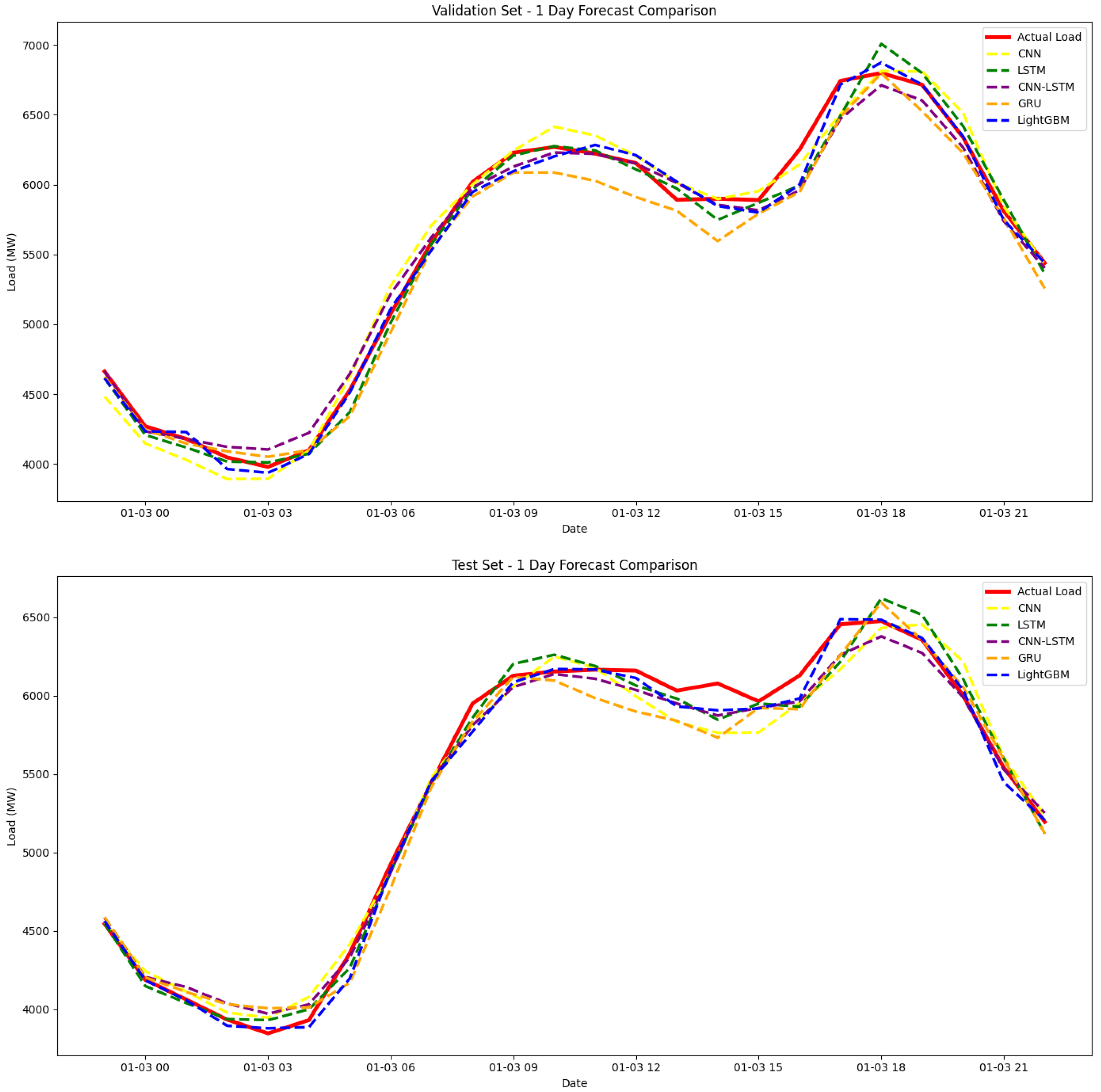
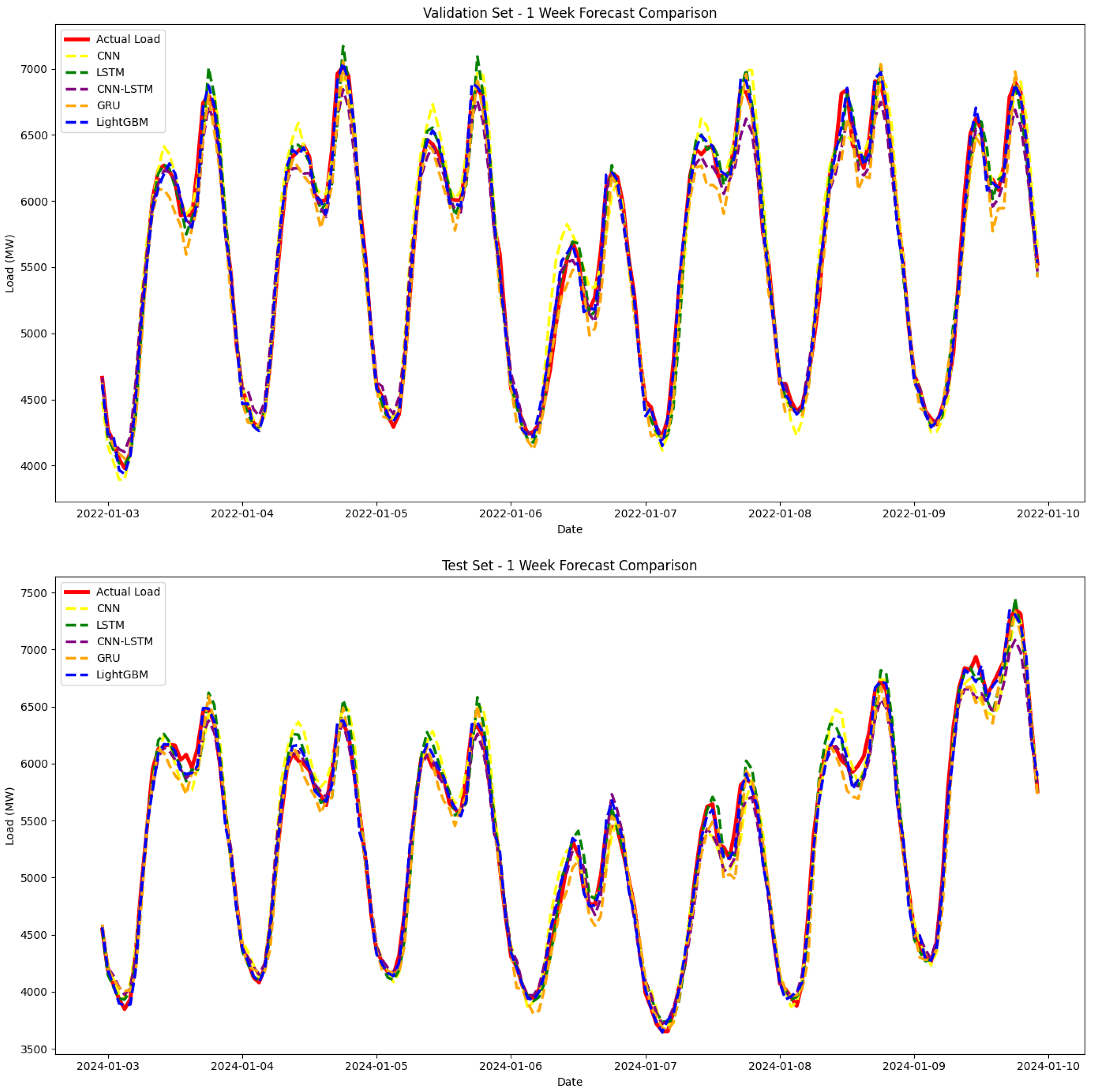
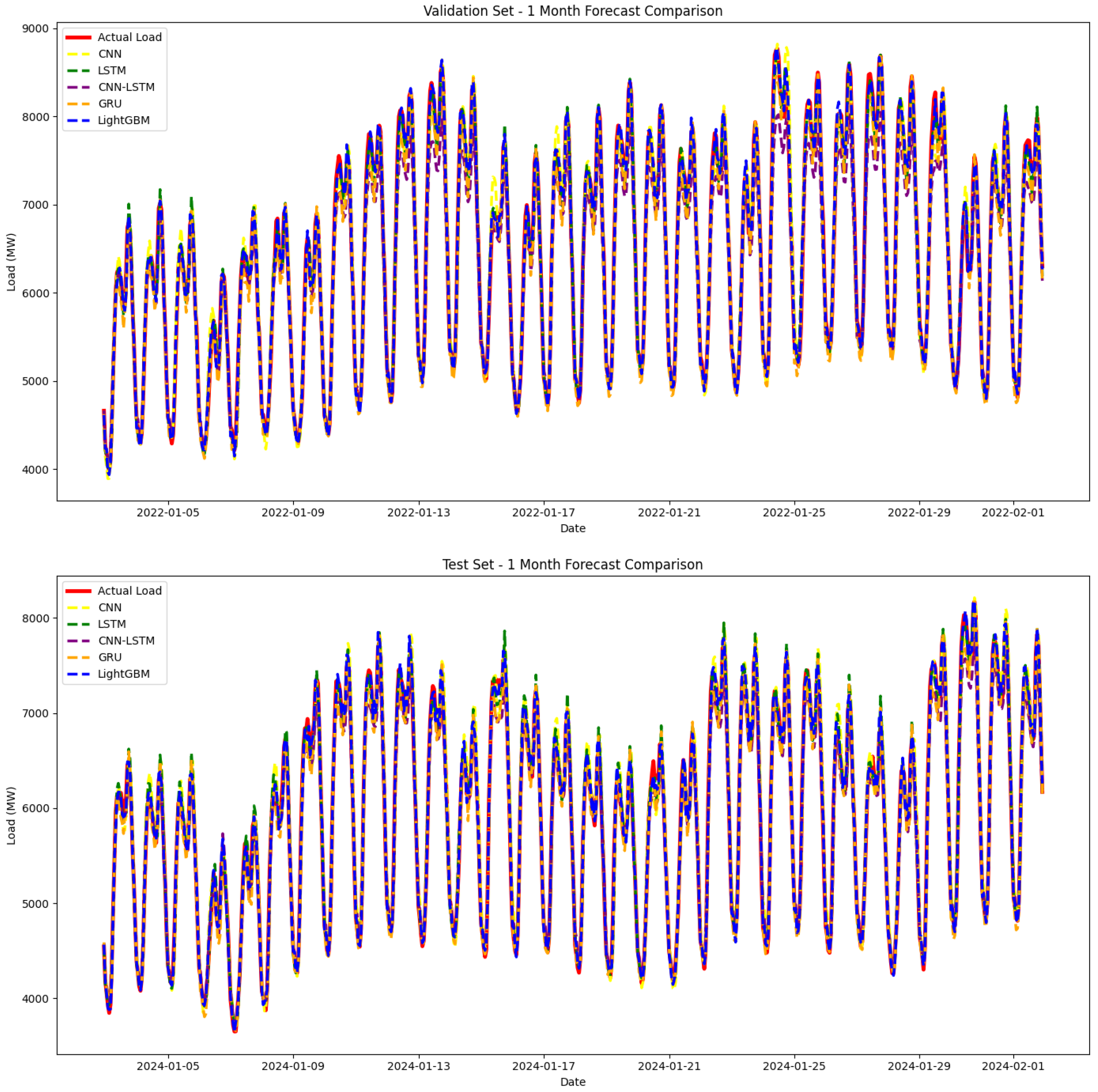
To further support the selection of LightGBM as the optimal model for short-term electricity load forecasting, a set of comparative visual analyses was conducted across different temporal resolutions and performance metrics, presented in Figure 13, Figure 14 and Figure 15. These figures showcase both model accuracy and robustness in varied conditions. Forecast curves for 1-day (Figure 13), 1-week (Figure 14), and 1-month (Figure 15) horizons further validate LightGBM’s performance. In all time windows, its predictions remained tightly aligned with the actual load values, exhibiting minimal deviation or temporal drift. Particularly during periods of high volatility—such as midday peaks or rapid demand changes—LightGBM consistently followed the actual signal more precisely than models like CNN, CNN-LSTM, or GRU. LSTM remained a close second, especially in short-horizon forecasts, but its performance slightly degraded during periods with high amplitude variance.
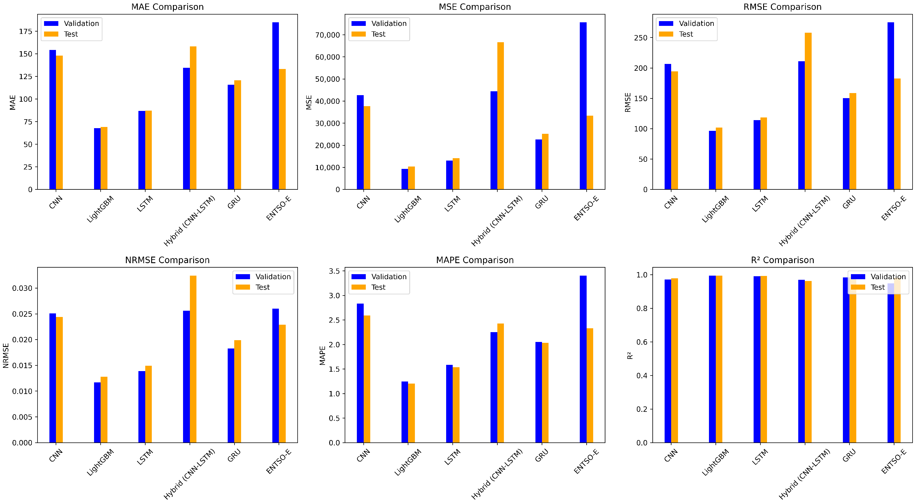
As shown in Figure 16, which presents a bar-wise comparison of error metrics across all models, LightGBM consistently outperformed the others for both the validation and test sets. It achieved the lowest scores for MAE, MSE, RMSE, MAPE, and NRMSE while also maintaining the highest R 2 values, indicating its exceptional accuracy and generalization capability. It is important to note that the actual electricity load values used in the forecasts were not scaled or normalized to a 0–1 range. Consequently, the absolute error values (particularly MAE, MSE, and RMSE) appear to be relatively high but are realistic and directly interpretable in megawatts (MWs), reflecting real-world forecasting performance.
While LSTM came closely behind LightGBM on some metrics—particularly R 2 and MAE—the noticeable gap in MSE and RMSE further reinforces LightGBM’s advantage in managing high-magnitude fluctuations and large-scale error suppression. These results confirm LightGBM’s suitability for operational deployment, where raw load values must be predicted accurately without the need for inverse normalization, making it not only the most accurate model but also the most practical for real-time forecasting applications.
Table 6 provides a comparative evaluation of the proposed LightGBM model against existing forecasting models reported in the literature and benchmarked data from the ENTSO-E platform. The first three models—ANN, Singular Value Decomposition (SVD)-ARIMA, and FF ANN—were sourced from prior research studies, while the ENTSO-E model represented forecast data obtained directly from the official ENTSO-E Transparency Platform. The performance of each model was assessed using standard metrics: MAE, MSE, RMSE, R 2 , MAPE, and NRMSE.
The ANN model produced an MAE of 112.92 MW and an MAPE of 1.92%, whereas the SVD-ARIMA hybrid model produced even larger error values, with an MAE of 220.53 MW and an RMSE of 267.39 MW, which indicates that it is not very suitable for highly dynamic load profiles. The FF ANN model did not provide full metrics but showed an NRMSE of 0.036 and an MAPE of 2.61%. The ENTSO-E forecast, evaluated using publicly available hourly forecasts, achieved an MAE of 133.31 MW, RMSE of 182.58 MW, R 2 of 0.9813, and MAPE of 2.33%, providing a realistic operational benchmark.
Conversely, the proposed LightGBM model outperformed all other models on every available metric. It had the best MAE (69.12 MW), MSE (10,335.78 MW), and RMSE (101.67 MW), along with the highest R 2 score (0.9942), which indicates excellent model fit and predictive power. Additionally, it had the lowest MAPE (1.20%) and NRMSE (0.0128), confirming that LightGBM provides accurate and scale-invariant forecasts.
This comparative analysis shows that LightGBM is not only superior to traditional and literature-based models but also outperforms the ENTSO-E operational benchmark, highlighting its practical applicability for real-world short-term electricity load forecasting.
In conclusion, among all evaluated models, LightGBM delivered the highest predictive accuracy, with the lowest error metrics and strongest generalization across datasets. Its ability to leverage engineered features without relying on complex sequence modeling makes it ideal for structured time-series tasks such as electricity load forecasting. LSTM ranked second, performing well in capturing temporal dependencies with minimal overfitting. In contrast, CNN, GRU, and CNN-LSTM demonstrated moderate accuracy but were more sensitive to data variability and less stable during high-volatility periods.
Overall, LightGBM offers the most accurate, efficient, and scalable solution for real-time operational deployment in short-term electricity load forecasting applications. Including models like ARIMA/SVR would not change the main ranking under our data scale since the computational burden of these models was the primary exclusion reason rather than lack of relevance.

4.3. Practical Deployment Challenges

While the models in this study perform well in terms of accuracy, their deployment in real-world smart grid environments faces several operational challenges:
  • Data Latency: LSTM, CNN, and hybrid (CNN-LSTM) models are more computationally intensive and may face delays in providing real-time predictions, particularly during periods of rapid demand changes. Minimizing latency in such cases is critical for operational decision-making.
  • Computational Cost: LSTM and CNN models require more computational power, which could be a barrier in smart grid environments with resource constraints. GRU, being computationally simpler, performs relatively better in terms of training time and inference speed. LightGBM stands out for its faster training time and lower memory requirements, making it suitable for real-time applications at scale.
  • Real-Time Constraints: Smart grids require frequent updates to forecasts based on incoming data. LSTM and hybrid (CNN-LSTM) models might require additional time to process and update their predictions, making them less ideal for applications where immediate decisions are critical. LightGBM, due to its feature-engineering approach and faster processing times, is better suited for real-time forecasting applications.
The above observations indicate that higher architectural complexity does not ensure better operational performance: in our experiments, LightGBM attained higher accuracy with lower latency and resource usage than the deep baselines. For applications where frequent model updates and tight real-time requirements are present, these trade-offs favour efficient boosting methods, unless domain-specific sequence effects justify the extra cost of deep recurrent or hybrid networks.
Finally, this section underscores the importance of selecting models that balance accuracy, computational efficiency, and real-time capabilities for operational deployment in smart grids.

4.4. Computational Efficiency Analysis

In addition to forecasting accuracy, we evaluated the computational efficiency of the five models in terms of training time, inference speed, and resource consumption. This aspect is particularly relevant for real-time operational deployment of load forecasting systems, where retraining speed and low-latency predictions are critical.
Table 7 summarizes the efficiency comparison. LightGBM completed full training in only 3.55 s on CPU (1000 boosting rounds, ∼60,000 samples) and achieved inference throughput of over 10,000 samples per second. The model also required minimal memory and produced a compact file size (<10 MB).
By contrast, DL models (LSTM, CNN, GRU, and CNN-LSTM) required 10–16 s per epoch on GPU, with total training times ranging from 8 to 18 min depending on the architecture. Their inference speeds were slower (approximately 2800–4500 samples per second) and memory consumption was significantly higher, particularly for the hybrid CNN-LSTM model due to its greater depth and parameter count.
The experimentation was conducted on the Kaggle platform using a 64-bit Linux operating system with an Intel(R) Xeon(R) CPU running at 2.00 GHz. The system was equipped with 2 Tesla T4 GPUs and 32 GB of RAM and Python 3.10.14 was used as the programming language.
These findings indicate that LightGBM not only outperformed all deep learning models in predictive accuracy but also delivered superior computational efficiency. This efficiency advantage makes LightGBM especially well-suited for large-scale or real-time STLF applications, where both speed and accuracy are critical.

5. Conclusions

This paper presented a comparative study of state-of-the-art ML and DL models for short-term load forecasting using Greek electricity demand data. The models tested included CNN, LSTM, GRU, a hybrid model (CNN-LSTM), and LightGBM. The results show that the LightGBM model outperforms all other models in terms of all standard error measures across various time horizons. Specifically, it achieved the best MAE (69.12 MW), MSE (10,335.78 MW2), RMSE (101.67 MW), MAPE (1.20%), and NRMSE (0.0128) and the highest R2 (0.9942), significantly surpassing other models and the ENTSO-E operational forecasts.
In comparison, the LSTM model demonstrated strong performance, with a test MAE of 87.26 MW, RMSE of 118.68 MW, MAPE of 1.53%, and R2 of 0.9921. However, it was not as effective as LightGBM, particularly in capturing high-magnitude fluctuations. The GRU and CNN models performed decently, with a test MAE of 120.64 MW (GRU) and 148.05 MW (CNN), but were less competitive in terms of accuracy. The hybrid CNN-LSTM model did not outperform its individual components, achieving a test MAE of 158.23 MW, RMSE of 258.05 MW, and R2 of 0.9628, suggesting potential redundancy or suboptimal integration.
These results emphasize that tabular models like LightGBM, combined with rich feature engineering (e.g., rich lagged and calendar features), can rival or even surpass DL architectures in structured forecasting tasks on the joint objectives of accuracy, generalization, and scalability. This is especially critical for real-time performance and interpretability in operational forecasting systems. Thus, practitioners should first exhaust strong tabular baselines (e.g., LightGBM with careful feature design and early stopping) before adopting recurrent or hybrid networks, which may introduce substantial complexity without reliable accuracy gains in high-variance regimes. Our scope is intentionally constrained to core, widely accessible variables to establish a reproducible baseline and isolate model effects. This design choice enhances comparability but does not capture behavioral demand response or renewable intermittency.
A key limitation of the present study is the use of Athens weather as a national proxy. While it captured dominant seasonal and peak patterns, it may have introduced bias regarding when regional weather diverges from that in the capital, possibly affecting model robustness. To address this, future work may incorporate spatially diverse meteorological inputs and reanalysis products to quantify any gains in accuracy and robustness. Furthermore, our feature-importance analysis indicated that humidity and holiday indicators have a relatively minor effect compared to temporal and lagged-load features; therefore, targeted ablation experiments are planned to substantiate and quantify these contributions more rigorously. Beyond point predictions, providing calibrated prediction intervals would enhance operational decision-making under renewable variability and is a natural extension of this work. Additionally, future research could extend this forecasting framework by integrating demand-side behavioral data, renewable energy generation patterns, and electricity pricing signals, thereby creating a more holistic energy forecasting system. Deploying the model in a real-time smart grid or distribution grid environment with streaming data would further assess its adaptability and scalability under live conditions. Finally, adapting the system for other European markets with different consumption behaviors could validate its generalizability and robustness across diverse energy systems.

Author Contributions

Conceptualization, M.F.H.S.; methodology, M.F.H.S. and P.K.; validation, M.F.H.S. and P.K.; formal analysis, M.F.H.S.; investigation, M.F.H.S. and P.K.; resources, M.F.H.S. and P.K.; data curation, M.F.H.S.; writing—original draft preparation, M.F.H.S.; writing—review and editing, M.F.H.S. and P.K.; visualization, M.F.H.S.; supervision, P.K.; project administration, P.K.; funding acquisition, P.K. All authors have read and agreed to the published version of the manuscript.

Funding

This research received no external funding.

Institutional Review Board Statement

Not applicable.

Informed Consent Statement

Not applicable.

Data Availability Statement

The datasets used for modeling in this study are openly available and can be extracted. Hourly power load: Available at https://transparency.entsoe.eu/ under the **Creative Commons Attribution (CC BY 4.0)** license (where applicable) (accessed on 10 July 2025). Hourly temperature and humidity: Can be retrieved from Python Meteostat API https://pypi.org/project/meteostat/ (accessed on 10 July 2025). Public holidays: Can be retrieved from Python holidays API https://pypi.org/project/holidays/ (accessed on 10 July 2025).

Acknowledgments

The authors would like to thank all the data providers and institutions whose open data repositories made this study possible.

Conflicts of Interest

The authors declare no conflicts of interest.

Abbreviations

The following abbreviations are used in this manuscript:
APIApplication Programming Interface
ARIMAAutoregressive Integrated Moving Average
ANNArtificial Neural Network
CNNConvolutional Neural Network
CNN-LSTMConvolutional Neural Network - Long Short-Term Memory
DBD-FELFDynamic Block-Diagonal Fuzzy Electric Load Forecaster
DLDeep Learning
EEMDEnsemble Empirical Mode Decomposition
EMDEmpirical Mode Decomposition
ENTSO-EEuropean Network of Transmission System Operators for Electricity
FF ANNFeed-Forward Artificial Neural Network
GBRGradient Boosting Regressor
GPUGraphics Processing Unit
GRUGated Recurrent Unit
IoTInternet of Things
KNNK-Nearest Neighbor
LightGBMLight Gradient Boosting Machine
LSTMLong Short-Term Memory
MAEMean Absolute Error
MAPEMean Absolute Percentage Error
MLMachine Learning
MSEMean Squared Error
MWMegawatt
MWhMegawatt-hour
NRMSENormalized Root Mean Squared Error
R 2 Coefficient of Determination
RBFNNsRadial Basis Function Neural Networks
RMSERoot Mean Squared Error
RNNsRecurrent Neural Networks
SSASingular Spectrum Analysis
STLFShort-Term Load Forecasting
SVRSupport Vector Regression
SVDSingular Value Decomposition
TLTransfer Learning
VSTLFVery Short-Term Load Forecasting
XGBoostExtreme Gradient Boosting Regressor

References

  1. Koukaras, P.; Mustapha, A.; Mystakidis, A.; Tjortjis, C. Optimizing building short-term load forecasting: A comparative analysis of machine learning models. Energies 2024, 17, 1450. [Google Scholar] [CrossRef]
  2. Ullah, K.; Ahsan, M.; Hasanat, S.M.; Haris, M.; Yousaf, H.; Raza, S.F.; Tandon, R.; Abid, S.; Ullah, Z. Short-term load forecasting: A comprehensive review and simulation study with CNN-LSTM hybrids approach. IEEE Access 2024, 12, 111858–111881. [Google Scholar] [CrossRef]
  3. Yuan, M.; Xie, J.; Liu, C.; Xu, Z. Short-term load forecasting for an industrial building based on diverse load patterns. Energy 2025, 334, 137481. [Google Scholar] [CrossRef]
  4. Junior, M.Y.; Freire, R.Z.; Seman, L.O.; Stefenon, S.F.; Mariani, V.C.; dos Santos Coelho, L. Optimized hybrid ensemble learning approaches applied to very short-term load forecasting. Int. J. Electr. Power Energy Syst. 2024, 155, 109579. [Google Scholar]
  5. Cheng, X.; Wang, L.; Zhang, P.; Wang, X.; Yan, Q. Short-term fast forecasting based on family behavior pattern recognition for small-scale users load. Clust. Comput. 2022, 25, 2107–2123. [Google Scholar] [CrossRef]
  6. Varelas, G.; Tzimas, G.; Alefragis, P. A new approach in forecasting Greek electricity demand: From high dimensional hourly series to univariate series transformation. Electr. J. 2023, 36, 107305. [Google Scholar] [CrossRef]
  7. Arvanitidis, A.I.; Bargiotas, D.; Daskalopulu, A.; Laitsos, V.M.; Tsoukalas, L.H. Enhanced short-term load forecasting using artificial neural networks. Energies 2021, 14, 7788. [Google Scholar] [CrossRef]
  8. Sideratos, G.; Ikonomopoulos, A.; Hatziargyriou, N.D. A novel fuzzy-based ensemble model for load forecasting using hybrid deep neural networks. Electr. Power Syst. Res. 2020, 178, 106025. [Google Scholar] [CrossRef]
  9. Stamatellos, G.; Stamatelos, T. Short-term load forecasting of the greek electricity system. Appl. Sci. 2023, 13, 2719. [Google Scholar] [CrossRef]
  10. Stratigakos, A.; Bachoumis, A.; Vita, V.; Zafiropoulos, E. Short-term net load forecasting with singular spectrum analysis and LSTM neural networks. Energies 2021, 14, 4107. [Google Scholar] [CrossRef]
  11. Kandilogiannakis, G.; Mastorocostas, P.; Voulodimos, A.; Hilas, C. Short-Term Load Forecasting of the Greek Power System Using a Dynamic Block-Diagonal Fuzzy Neural Network. Energies 2023, 16, 4227. [Google Scholar] [CrossRef]
  12. Stergiou, K.; Karakasidis, T.E. Application of deep learning and chaos theory for load forecasting in Greece. Neural Comput. Appl. 2021, 33, 16713–16731. [Google Scholar] [CrossRef]
  13. Tzortzis, A.M.; Pelekis, S.; Spiliotis, E.; Karakolis, E.; Mouzakitis, S.; Psarras, J.; Askounis, D. Transfer learning for day-ahead load forecasting: A case study on European national electricity demand time series. Mathematics 2023, 12, 19. [Google Scholar] [CrossRef]
  14. Panapakidis, I.P.; Skiadopoulos, N.; Christoforidis, G.C. Combined forecasting system for short-term bus load forecasting based on clustering and neural networks. IET Gener. Transm. Distrib. 2020, 14, 3652–3664. [Google Scholar] [CrossRef]
  15. Katya, E. Exploring Feature Engineering Strategies for Improving Predictive Models in Data Science. Res. J. Comput. Syst. Eng. 2023, 4, 201–215. [Google Scholar] [CrossRef]
  16. Murti, D.M.P.; Pujianto, U.; Wibawa, A.P.; Akbar, M.I. K-Nearest Neighbor (K-NN) based Missing Data Imputation. In Proceedings of the 2019 5th International Conference on Science in Information Technology (ICSITech), Yogyakarta, Indonesia, 23–24 October 2019; pp. 83–88. [Google Scholar] [CrossRef]
  17. Bichri, H.; Chergui, A.; Hain, M. Investigating the Impact of Train/Test Split Ratio on the Performance of Pre-Trained Models with Custom Datasets. Int. J. Adv. Comput. Sci. Appl. 2024, 15, 2. [Google Scholar] [CrossRef]
  18. Wang, C.; Li, X.; Shi, Y.; Jiang, W.; Song, Q.; Li, X. Load forecasting method based on CNN and extended LSTM. Energy Rep. 2024, 12, 2452–2461. [Google Scholar] [CrossRef]
  19. Jalali, S.M.J.; Ahmadian, S.; Khosravi, A.; Shafie-khah, M.; Nahavandi, S.; Catalão, J.P.S. A Novel Evolutionary-Based Deep Convolutional Neural Network Model for Intelligent Load Forecasting. IEEE Trans. Ind. Inform. 2021, 17, 8243–8253. [Google Scholar] [CrossRef]
  20. Koukaras, P.; Bezas, N.; Gkaidatzis, P.; Ioannidis, D.; Tzovaras, D.; Tjortjis, C. Introducing a novel approach in one-step ahead energy load forecasting. Sustain. Comput. Inform. Syst. 2021, 32, 100616. [Google Scholar] [CrossRef]
  21. Alhussein, M.; Aurangzeb, K.; Haider, S.I. Hybrid CNN-LSTM model for short-term individual household load forecasting. IEEE Access 2020, 8, 180544–180557. [Google Scholar] [CrossRef]
  22. Yunita, A.; Pratama, M.I.; Almuzakki, M.Z.; Ramadhan, H.; Akhir, E.A.P.; Firdausiah Mansur, A.B.; Basori, A.H. Performance analysis of neural network architectures for time series forecasting: A comparative study of RNN, LSTM, GRU, and hybrid models. MethodsX 2025, 15, 103462. [Google Scholar] [CrossRef]
  23. Park, J.; Hwang, E. A two-stage multistep-ahead electricity load forecasting scheme based on LightGBM and attention-BiLSTM. Sensors 2021, 21, 7697. [Google Scholar] [CrossRef]
  24. Nti, I.K.; Teimeh, M.; Nyarko-Boateng, O.; Adekoya, A.F. Electricity load forecasting: A systematic review. J. Electr. Syst. Inf. Technol. 2020, 7, 13. [Google Scholar] [CrossRef]
  25. Steurer, M.; Hill, R.J.; Pfeifer, N. Metrics for evaluating the performance of machine learning based automated valuation models. J. Prop. Res. 2021, 38, 99–129. [Google Scholar] [CrossRef]
  26. Tanoli, I.K.; Mehdi, A.; Algarni, A.D.; Fazal, A.; Khan, T.A.; Ahmad, S.; Ateya, A.A. Machine learning for high-performance solar radiation prediction. Energy Rep. 2024, 12, 4794–4804. [Google Scholar] [CrossRef]
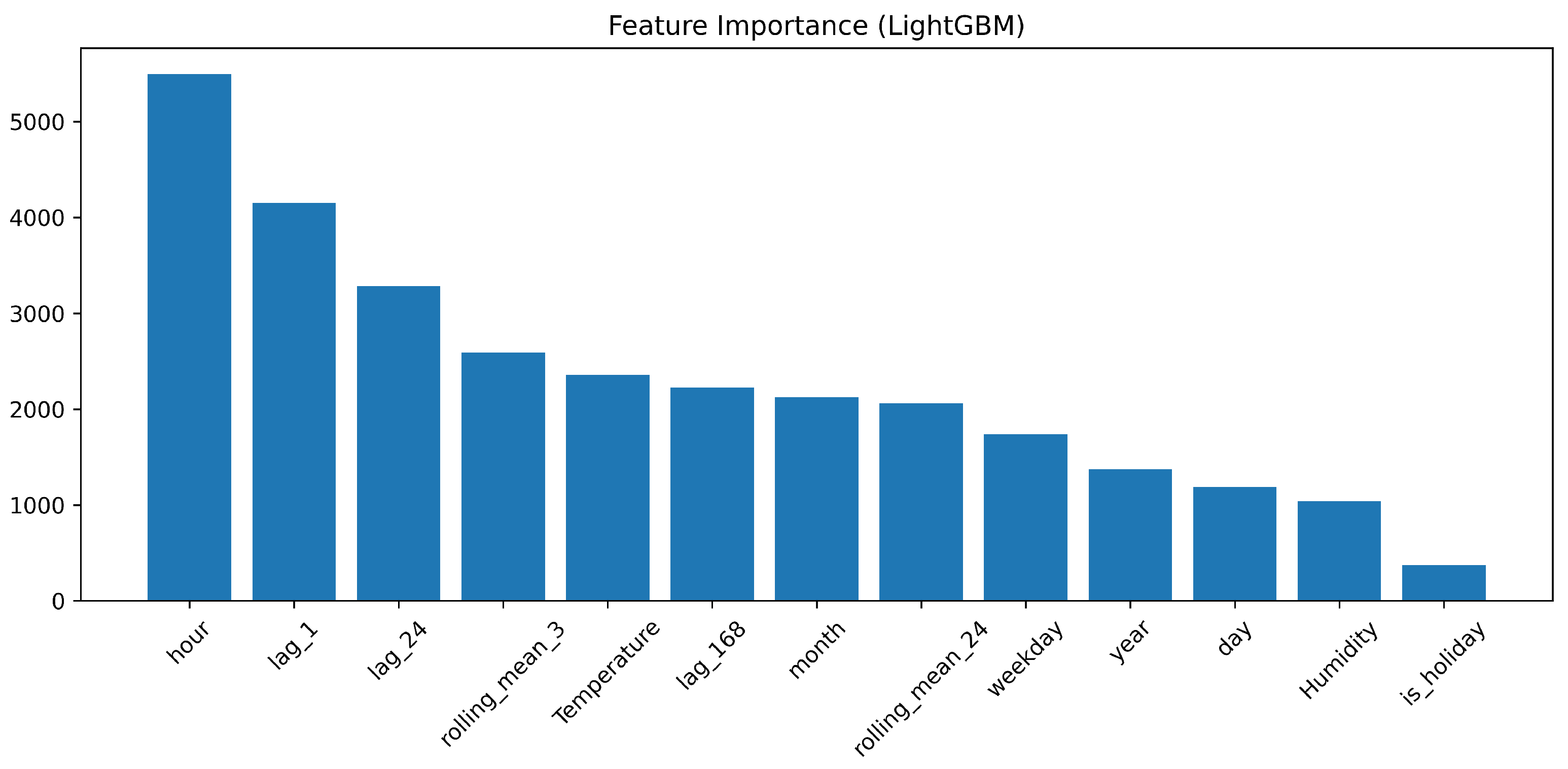
Figure 1. Feature importance plot for LightGBM model on short-term load forecasting.
Energies 18 05060 g001
Figure 2. Workflow of experimental setup: data preprocessing, model training, and evaluation.
Energies 18 05060 g002
Figure 3. Daily mean forecast vs. actual load using theCNN model on the validation and test sets.
Energies 18 05060 g003
Figure 4. Hourly forecast vs. actual load using the CNN model on validation and test sets.
Energies 18 05060 g004
Figure 5. Daily mean forecast vs. actual load using the LSTM model on validation and test sets.
Energies 18 05060 g005
Figure 6. Hourly forecast vs. actual load using the LSTM model on validation and test sets.
Energies 18 05060 g006
Figure 7. Daily mean forecast vs. actual load using the hybrid model on validation and test sets.
Energies 18 05060 g007
Figure 8. Hourly forecast vs. actual load using the hybrid model on validation and test sets.
Energies 18 05060 g008
Figure 9. Daily mean forecast vs. actual load using the GRU model on validation and test sets.
Energies 18 05060 g009
Figure 10. Hourly forecast vs. actual load using the GRU model on validation and test sets.
Energies 18 05060 g010
Figure 11. Daily mean forecast vs. actual load using the LightGBM model on validation and test sets.
Energies 18 05060 g011
Figure 12. Hourly forecast vs. actual load using the LightGBM model on validation and test sets.
Energies 18 05060 g012
Figure 13. One-day forecast comparison (validation and test sets).
Energies 18 05060 g013
Figure 14. One-week forecast comparison (validation and test sets).
Energies 18 05060 g014
Figure 15. One-month forecast comparison (validation and test sets).
Energies 18 05060 g015
Figure 16. Error metric comparison across all models (validation and test sets).
Energies 18 05060 g016
Table 1. CNN model performance metrics.
MetricTrainValidationTest
MAE126.8867154.0706148.0502
MSE31,255.757142,715.062637,676.0284
RMSE176.7930206.6762194.1031
R 2 0.97630.97060.9789
MAPE (%)2.20222.83682.5900
NRMSE0.02350.02510.0244
Table 2. LSTM model performance metrics.
MetricTrainValidationTest
MAE92.224986.730587.2611
MSE17,917.367713,067.978514,085.0742
RMSE133.8558114.3153118.6806
R 2 0.98640.99100.9921
MAPE (%)1.59731.58701.5339
NRMSE0.01780.01390.0149
Table 3. Hybrid (CNN-LSTM) model performance metrics.
MetricTrainValidationTest
MAE139.1704134.6142158.2293
MSE44,559.405644,445.230366,591.6128
RMSE211.0910210.8204258.0535
R 2 0.96620.96940.9628
MAPE (%)2.19212.24962.4263
NRMSE0.02800.02560.0324
Table 4. GRU model performance metrics.
MetricTrainValidationTest
MAE127.2923115.6403120.6414
MSE29,515.282322,622.520125,217.7061
RMSE171.8001150.4078158.8008
R 2 0.97760.98440.9859
MAPE (%)2.14912.05082.0330
NRMSE0.02280.01830.0199
Table 5. LightGBM model performance metrics.
MetricTrainValidationTest
MAE45.511467.806569.1205
MSE4644.32779260.645610,335.7831
RMSE68.149396.2322101.6651
R 2 0.99650.99360.9942
MAPE (%)0.80221.24501.2025
NRMSE0.00900.01170.0128
Table 6. Performance comparison with existing models from the literature.
MetricANN
[7]
SVD-ARIMA
[6]
FF ANN
[9]
ENTSO-ELightGBM
MAE112.9198220.5342-133.307269.1205
MSE22,111.6668--33,334.429810,335.7831
RMSE-267.3871-182.5771101.6651
R 2 ---0.98130.9942
MAPE (%)1.924.32862.612.32821.2025
NRMSE--0.0360.02290.0128
Table 7. Comparison of computational efficiency across models.
ModelTraining TimeInference SpeedResource Usage
LightGBM3.55 s (CPU)>10,000/sLow, <10 MB
CNN∼8 min (GPU)∼4500/sModerate
LSTM∼12 min (GPU)∼3200/sHigh
GRU∼10 min (GPU)∼3600/sMedium
CNN-LSTM∼18 min (GPU)∼2800/sHighest
Disclaimer/Publisher’s Note: The statements, opinions and data contained in all publications are solely those of the individual author(s) and contributor(s) and not of MDPI and/or the editor(s). MDPI and/or the editor(s) disclaim responsibility for any injury to people or property resulting from any ideas, methods, instructions or products referred to in the content.