Abstract
Fair sharing of carbon emission responsibilities is an important direction for the low carbonization of power systems. This paper proposes a new low-carbon dispatch method (N-LCD), which takes node carbon emissions as a constraint for power system decision-making, so as to adapt to the current management needs of power carbon footprint. The N-LCD model is built on the traditional optimal power flow (OPF) or low-carbon dispatch (LCD) model, integrating carbon flow equations and constraints and introducing a bidirectional power flow component to solve the problem of unknown carbon flow direction in power flow optimization. Empirical analysis proves the effectiveness of the N-LCD model in ensuring the fair share of carbon emission responsibilities and solving low-carbon unit commitment optimization based on carbon nodal emission control.
1. Introduction
In recent years, energy efficiency and carbon emissions have garnered significant global attention due to their critical role in climate mitigation [1]. As the most critical sector of the energy system [2], the transparency and precise quantification of carbon emission responsibility in power systems form an essential foundation for carbon emission control [3]. Although direct carbon emissions in power systems almost exclusively originate from fossil fuel combustion in power generation units, the combustion activities of these units are closely tied to electricity demand from end-users [4]. Meanwhile, it is also necessary to consider that low-carbon dispatch should also ensure the security of the power system [5,6]. Therefore, fairly allocating carbon emission responsibility to the demand side is a crucial pathway to addressing rising carbon emissions in power systems.
To meet carbon reduction requirements in the power sector, it is necessary to coordinate relationships between different types of power generation to establish synergistic effects conducive to emission reduction. Low-carbon power dispatch (LCD) has been widely recognized as one of the most effective approaches to achieving this goal. To our knowledge, common LCD models usually adopt the method of adding carbon emission penalty terms to the objective function [7] or compare different carbon emissions under multiple preset scenarios to select the scheduling method with lower carbon emissions [8]. Recently, many studies [9,10] have incorporated carbon emission flows into power system planning and operation. Li et al. [11] proposed a method for calculating IES carbon emission flow considering energy quality. Zhu et al. [12] set up a stochastic multi-objective sizing optimization (SMOS) model for microgrid planning, which fully captures the total carbon emissions in microgrid servers. Zhang et al. [13] investigated the low-carbon operation of multi-energy systems and reduced carbon emissions through electric vehicle charging methods and carbon trading mechanisms. However, in the aforementioned decision-making processes, carbon emission flows are typically calculated recursively after power flow dispatch, with little emphasis on constraining demand-side carbon footprints. Under current carbon–electricity market mechanisms, node-level carbon emission constraints can better reflect the impact of proactive emission reduction efforts by end-users on the power system.
In this paper, we introduce a nodal carbon emission flow-based generation scheduling method (N-LCD) to achieve day-ahead low-carbon scheduling with embedded carbon emission flow. This is the first time that nodal carbon emission flow theory has been incorporated into the active management of the grid’s carbon footprint as the basis for carbon-aware decision-making in the power system. The N-LCD model is built upon the traditional optimal power flow (OPF) model, further integrating carbon flow equations, constraints, and carbon-related objectives to limit carbon flows and optimize power flows in the grid. Essentially, N-LCD is a carbon-aware generalization of OPF, producing optimal decisions that satisfy carbon emission limits while balancing power-related and carbon-related costs. This gives the N-LCD model a new advantage: it can calculate the real power flow under any given carbon emission limit.
To our knowledge, this study is the first to address low-carbon unit commitment optimization using embedded carbon emission flow theory and considering the unit start-up and shutdown issues. Existing low-carbon optimization frameworks primarily focus on economic dispatch, which is not good at addressing unit commitment issues under the significant volatility of distributed renewable energy outputs. In our model, the node emission reduction amount is used as a constraint condition to obtain the lowest-cost unit output combination under the emission reduction conditions to meet the carbon emission reduction needs of users at this node. The proposed method further supplements existing carbon emission flow theories and provides a refined strategy for carbon emission control in power systems. It offers an optimal economic dispatch model that complies with carbon emission policies, particularly suitable for multi-energy-coupled industrial parks. The main contributions of this work are as follows:
- (1)
- An optimization scheduling model based on carbon emission flow theory is proposed. Under this model, carbon emission is allowed to participate in flow optimization as a constraint condition, thereby achieving node carbon emission or overall carbon emission control.
- (2)
- A method for reformulating the flow is proposed to solve the problem of unknown flow direction in the traditional carbon flow model by introducing dual flow variables.
2. Carbon Emission Flow Theory
The widespread long-term application of the Average Emission Factor (AEF) across global power systems is currently limited by insufficient temporal and spatial granularity [14]. As the integration of renewable energy sources, such as wind and solar power, continues to increase, the power generation profile within future power systems will exhibit pronounced seasonal, regional, and temporal variations [15]. A foundational theoretical framework for allocating carbon emission responsibility within power systems was established by Kang et al. [16], conceptualizing carbon emissions as a virtual flow embedded within energy streams that propagate from producers to consumers. Building upon this, Zhou et al. [17,18] formalized the core concept of carbon emission flow (CEF) in power systems. These studies defined key CEF metrics, including branch carbon flow rate, grid loss carbon flow rate, and nodal carbon intensity. Furthermore, they developed a methodology for calculating CEF based on power flow analysis and investigated the distribution characteristics and transmission mechanisms of CEF within electrical networks [19]. Building on this, Kang et al. [20] incorporated a recursive approach into carbon emission flow calculations, using the carbon emission intensity of the generation side as boundary conditions to sequentially determine the carbon emission factors for all nodes in the network. In this way, the carbon flow method serves as an important tool for demand-side carbon accounting, aligning carbon footprint calculations with the physical power grid and electricity flows. Compared to the AEF, the carbon emission flow algorithm can compute high spatiotemporal-resolution carbon emission factors based on high-frequency power flow data, enabling precise quantification of carbon emission responsibilities for different types of users across various time periods. This lays the theoretical groundwork for allocating carbon emission responsibility based on actual energy flows.
CEF is a responsibility allocation framework that conceptualizes carbon emissions as virtual labels attached to power flows. This approach enables the explicit tracing of emission transmission and accumulation within power grids. Traditional regional carbon accounting methods uniformly allocate carbon responsibility to all users within a geographical boundary, irrespective of their actual energy consumption profiles. For instance, users relying on clean energy sources (e.g., solar, wind) are assigned the same carbon responsibility as those consuming fossil fuels (e.g., coal, natural gas), which fails to incentivize low-carbon energy adoption. In contrast, CEF decouples carbon responsibility from subjective regional divisions by basing its calculations on the objective physical distribution of power flows. While preserving the fairness principle of averaging energy consumption, CEF applies this principle specifically to users sharing identical energy consumption patterns.
3. N-LCD Optimization Model
3.1. Electricity Carbon Emission Flow Model Based on Active Power
Consider a power network with nodes and a topological set . Let (kg/h) denote the carbon emission flow and (kg/kWh) represent the nodal carbon intensity, defined as , which quantifies the CO2 responsibility per unit of electricity. Since carbon flows strictly follow an active power distribution, a DC power flow model is adopted for computational efficiency. Each node must satisfy the power balance equation:
where and denote branch flows from node n to i and i to j, respectively (outflows: positive; inflows: negative). and represent generator outputs and loads at node i. In order to facilitate the resolution of the issue, this model exclusively addresses the transmission of active current, while disregarding the current loss attributable to network loss. In the context of a virtual material flow, the inflow and outflow of carbon emissions must also adhere to the law of conservation of matter. Carbon flows adhere to conservation principles:
where and denote branch carbon flows from node n to i and i to j, respectively (outflows: positive; inflows: negative). and represent generator outputs and loads at node i.
There is usually a consensus on carbon responsibility sharing that electricity exported from the same node should have the same carbon emission factor. Under this fairness-mixing principle, all outflows from a node share the same carbon intensity, which is equal to the node’s carbon emission factors . Therefore, Equation (2) can be rewritten as
represents the carbon emission factor of the generating units connected to node i. represents the carbon emission factor of node i, which applies to load and output flows at node i. Combining Equations (1) and (3), the nodal carbon intensity is derived as
A critical challenge arises in determining inflow carbon intensities when power flow directions are indeterminate. To resolve this, we adopt the graph-theoretical approach proposed by Chen et al. [21], introducing non-negative flow components and :
is defined as the power flow from node i to node j in branch l. is defined as the flow in the opposite direction. Since the power flow is only allowed to exist in one direction, there must be one flow component equal to zero:
Combining Equations (6) and (7), we can further relax Equation (8):
Based on the complete definition above, we now multiply the denominator in Equation (4) by the left side of the equation and replace the flow with the flow components and . Equation (4) can be rewritten as
Since there is only one flow direction for the load and the generator set, it is not necessary to replace and for the flow component. This method breaks down the power current flowing to i into all the flows connected to node i, which drastically simplifies the difficulty of modeling in the computation.
3.2. Cost Minimization Function
For hybrid power systems comprising thermal, wind, and photovoltaic (PV) units, the total generation cost () is formulated as a quadratic function to capture the nonlinear relationship between power output and operational expenses:
, , and are the quadratic cost coefficient, linear cost coefficient, and fixed cost coefficient of the output fitting of the generator set g.
Based on the conservation of total carbon emissions, the cost of carbon emissions at each node of the power system can be calculated on the source side. The carbon emission cost is integrated as an additive term into the total cost function, proportional to the carbon intensity () of each generator:
represents the cost per ton of carbon emissions and represents the linear cost coefficient correction term.
Normally, we consider the cost factor of wind power () and photovoltaic power () generation to be 0 because the process of power generation does not require the consumption of fuel and the operation and maintenance costs can be regarded as fixed costs.
3.3. Power System Constraints
In Section 3.1 and Section 3.2, we have provided the constraints and objective functions related to carbon flow. Now we will discuss other relevant power system constraints in detail:
3.3.1. System Power Balance Constraints
The production, transmission, and consumption of electrical energy take place almost simultaneously, and the sum of all unit outputs must be equal to the sum of the total system load and network losses in a system without the participation of energy storage devices. Without taking into account the network losses, the system power balance equation can be expressed as follows:
3.3.2. PTDF (Power Transfer Distribution Factor) Constraints
PTDF is a matrix that describes the effect of active power injection on the actual power flow [22]. Since the carbon emission flow is only transmitted along with the active power flow, the DC power calculation method based on the power transfer distribution factor can simplify the network parameters of the grid, thus quickly calculating the power flow. Pin is the injected power matrix of all nodes.
3.3.3. Generator Set Output Constraints
When the unit is running, the output must meet the upper and lower limit restrictions; when it is shut down, the unit output must be 0.
where and denote upper and lower output limits of unit i.
3.3.4. Ramp Rate Constraints
Generation units, especially coal-fired units, are subject to physical limitations such as boiler heating and steam turbine inertia, which prevent their power output from changing drastically within a single time period. Therefore, ramp rate constraints must be applied to restrict output variations.
3.3.5. Minimum Start and Stop Time Constraints
Due to the technical requirements of boilers and steam turbines, once a generation unit is started, it must operate continuously for a certain period and cannot be shut down immediately. Similarly, after shutdown, the unit must remain offline for a specified duration before restarting. Therefore, thermal power unit generation scheduling must satisfy minimum uptime and downtime constraints.
3.3.6. Spinning Reserve Constraints
In practical power systems, unplanned events such as random load fluctuations and unexpected equipment failures frequently occur. To ensure power supply security and reliability, the system must maintain a certain reserve capacity to handle these uncertainties. Reserves can be categorized into three types based on their purposes: load reserve, maintenance reserve, and emergency reserve. Among these, the load reserve and part of the emergency reserve must be immediately available to respond to system load variations; hence they are also referred to as hot reserve or spinning reserve. The remaining portion of these reserves is generally called cold reserve.
where denotes the total reserve capacity at time t.
However, in power systems with significant renewable energy integration, reserve requirements must account not only for load fluctuations but also for renewable generation variability. Therefore, under more refined considerations, we propose that both upward and downward reserve requirements from thermal power units should be incorporated.
In practical operations, since it is impossible to mitigate renewable forecast deviations exceeding the coal power’s ramp down limits through curtailment alone, the parameters and can be appropriately relaxed during configuration. Furthermore, reserve capacity calculations that disregard unit commitment status and ramp rate limitations may exceed the system’s actual operational capabilities. A more refined approach would be to evaluate the real-time available reserve capacity the system can provide at any given moment.
In the formula, represents conventional energy units.
3.4. Carbon Emission Constraints
In conventional economic dispatch, total carbon emissions are typically constrained. Existing methods for calculating system-wide carbon emissions generally consider only generation-side emissions from power units. Under carbon flow equation constraints, the following condition should be satisfied:
Under the assumptions of neglecting network losses and excluding energy storage participation, constraining either generation-side or load-side carbon emissions can achieve total carbon emission targets.
There is also consideration of nodal carbon emission factor constraints.
However, implementing constraints based on nodal carbon emission factors presents a significant contradiction: such constraints would clearly be unattainable for coal-dominated nodes, as the high emission factors of large-capacity coal power nodes leave virtually no possibility for alternative power flows to reach these nodes. A viable improvement would be to narrow the scope by applying the constraints specifically to load nodes.
This can be achieved by setting distinct carbon emission factors for different nodes. However, this approach presents a potential contradiction with actual industrial practices, where regulatory policies typically target a company’s total carbon emissions rather than emission factors. In other words, companies are required to reduce their aggregate carbon emissions, rather than ceasing all production activities during periods of renewable energy scarcity.
Thanks to the optimized carbon flow equations that resolve the constraints of nodal carbon emissions, our model can incorporate nodal-level total carbon emission controls:
A feasible approach is to first compute the initial carbon emissions under a pure economic dispatch as the constraint reference value, then progressively tighten the constraints. This process better aligns with real-world industrial practices where companies purchase green electricity to reduce their carbon footprint. However, it should be noted that in actual operations, the power flow corresponding to green electricity purchases may not necessarily satisfy physical transmission constraints. There could exist cases where the purchased green electricity volume exceeds physical transmission limits. Our model, based on physical power flow-constrained unit commitment, can only address transmission issues under limited green electricity procurement scenarios.
4. Example Demonstration
4.1. Scene Set Up
Our simulations employ a 24 h day-ahead economic dispatch framework with hourly resolution, utilizing the modified PJM-5 bus test system illustrated in Figure 1 This system configuration comprises two coal-fired units, one gas-fired unit, one wind farm, one solar plant, and three load centers. Prior to detailed analysis, we outline the core model configuration comprising three load nodes—L1 (industrial, high-demand), L2, and L3—where carbon emission controls apply exclusively to L1. The generation portfolio includes G1 (wind), G2 (PV), G3 (gas), and coal units G4–G5, with detailed parameters documented in the Supplementary Material. Key assumptions disregard transmission losses and consider only active power flow calculations. Three simulation scenarios were designed: the baseline scenario implements unconstrained carbon emissions through pure economic dispatch; the system-wide carbon cap scenario imposes 1–6% incremental emission reductions relative to baseline levels; and the nodal carbon cap scenario enforces equivalent 1–6% reductions solely on emissions originating from L3. Additional parameter specifications are provided in the paper’s Supplementary Material, and the model employs Gurobi’s commercial solver for optimization.
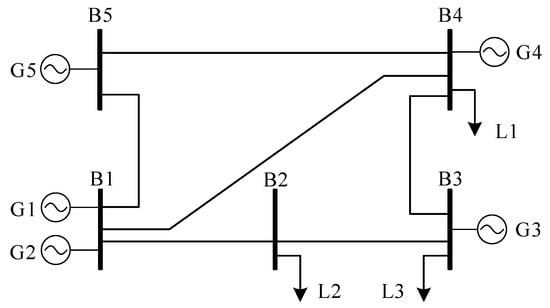
Figure 1.
PJM5 bus power system.
4.2. Example Analysis
As shown in Figure 2, renewable energy generation—specifically solar and wind power—is fully utilized without curtailment in all decision scenarios. The primary distinction lies in how the system progressively replaces low-cost, high-emission, coal-fired generation with cleaner alternatives like natural gas as carbon emission limits tighten, thereby reducing overall system emissions.
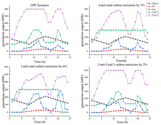
Figure 2.
Power outputs of different scenarios.
In Figure 3, the 24 h variation in load-side carbon emission flows reveals that emissions generally follow the load curve distribution. Notably, as carbon emission flows serve as virtual labels of physical power flows, their total volume closely correlates with power flow directions. Although Loads 1 and 2 are both adjacent to wind/solar nodes and lack transmission limits and Load 2 has higher demand than Load 1, Load 2 assumes greater carbon responsibility during high renewable-output periods due to power flow routing. Overall, carbon emission flow distribution exhibits a clear positive correlation with load distribution, with significant emission reductions during peak renewable generation intervals.
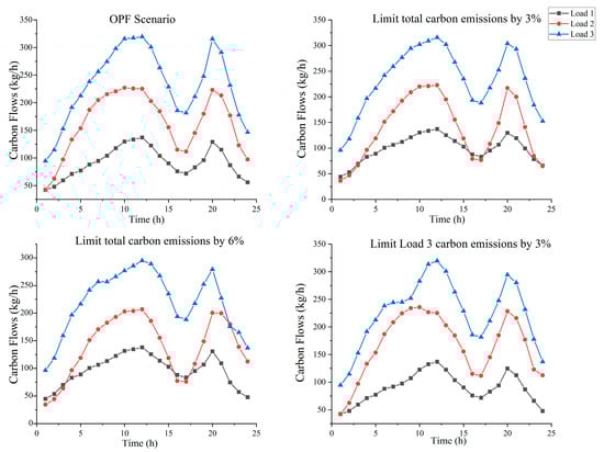
Figure 3.
Carbon flows of different scenarios.
In Figure 4, stricter carbon constraints lead to nonlinear cost increases, indicating that initial emission reductions prioritize substitution among coal-fired units, while gas-for-coal replacement occurs only under tighter constraints. This phased substitution sequence causes temporary emission increases at some nodes during early constraint stages. In contrast, single-node carbon constraints yield more linear cost growth and smoother transitions in energy substitution ratios.
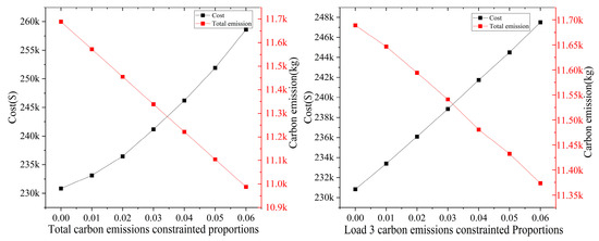
Figure 4.
Total cost and carbon emission curve.
By applying different levels of carbon emission constraints, we found that imposing system-wide carbon caps does not lead to simultaneous emission reductions across all nodes as shown in Figure 5. Instead, due to changes in unit dispatch, nodes adjacent to renewable (wind/PV) units may receive more renewable power flows, while emissions at other nodes could increase. Therefore, when implementing system-wide carbon constraints, it is essential to fully consider the carbon emission entitlements of all enterprises within the planning area. Here, we advocate for constraining total emissions at individual nodes instead. When applying single-node constraints, it can be observed that emissions at Load 2 gradually increase while emissions at Loads 1 and 3 steadily decrease, with overall system emissions also declining. This occurs because the system adjusts generator outputs, redirecting renewable energy carbon flows that originally prioritized Load 2 toward Load 3—the opposite of what happens under system-wide constraints, where all generator outputs prioritize supplying neighboring nodes.
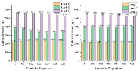
Figure 5.
Constraint intensity and carbon emissions.
Under system-wide carbon constraints, maintaining conventional unit dispatch practices actually leads to inequitable distribution of carbon responsibility among loads. Nodes near wind power installations but without generation units will see significantly reduced carbon accountability, as power flow characteristics will direct large amounts of renewable energy to these nodes, even though these nodes may not actually bear higher carbon costs. However, when nodal constraints are implemented, unit dispatch does not simply increase low-carbon generation at constrained nodes but rather redistributes outputs to direct more green power flows toward nodes willing to pay higher carbon costs—which aligns perfectly with the principles of green electricity trading. The above results show that we should pay attention to the location of high-emission industries or adopt the direct power supply method to obtain green electricity.
5. Conclusions
In summary, this paper proposes an innovative unit dispatch approach—a generation scheduling scheme based on nodal carbon emission constraints. This approach addresses the problem of embedding carbon emission flows into low-carbon scheduling. Building upon previous research, we developed a low-carbon dispatch model incorporating mixed-unit commitment characteristics, which simulates nodal green electricity procurement scenarios (i.e., setting specific percentage reduction targets for individual nodes) to investigate carbon flow distribution changes in power systems. Comparative analysis reveals that when applying single-node constraints, the system preferentially reallocates green power flows, resulting in increased emissions at originally green-energy-receiving nodes while reducing emissions at purchasing nodes, simultaneously achieving overall emission reduction through energy substitution effects. Conversely, directly imposing carbon constraints on all nodes may exacerbate inter-nodal carbon responsibility allocation imbalances due to geographical factors, ultimately increasing the actual emission burden on target nodes. Therefore, we believe the N-LCD model can accurately predict the availability of corresponding unit outputs in actual production to meet pre-defined emission reduction plans. When we input the desired carbon emission reduction constraint, N-LCD attempts to determine whether a unit output satisfies this constraint and finds the lowest cost. We believe this represents a novel low-carbon scheduling approach that integrates node carbon emission flows.
Supplementary Materials
The following supporting information can be downloaded at https://www.mdpi.com/article/10.3390/en18195050/s1: Table S1: Generator cost factors and carbon factors; Table S2: Coal-fired power unit parameters at node 4; Table S3: Coal-fired power unit parameters at node 5; Table S4: PTDF calculation.
Author Contributions
Conceptualization, X.W. and Q.C.; methodology, W.Z.; validation, J.X.; investigation, D.X.; data curation, H.C.; writing—original draft preparation, X.W. and X.Y.; writing—review and editing, Q.C. and C.Y. All authors have read and agreed to the published version of the manuscript.
Funding
This research was funded by State Grid Fujian Electric Power Company Information and Communication Branch, grant number 52130M23000S.
Data Availability Statement
The data presented in this study are available on request from the corresponding author. The data are not publicly available due to privacy.
Conflicts of Interest
Authors Xi Wu, Weitao Zheng, Jingyu Xie, Danhong Xie, Hancheng Chen and Xiang Yu were employed by the company State Grid Fujian Electric Power Company Information and Communication Branch. The remaining authors declare that the research was conducted in the absence of any commercial or financial relationships that could be construed as a potential conflict of interest.
References
- Bodansky, D. The Legal Character of the Paris Agreement. Rev. Eur. Comp. Int. Environ. Law 2016, 25, 142–150. [Google Scholar] [CrossRef]
- Bogdanov, D.; Gulagi, A.; Fasihi, M.; Breyer, C. Full energy sector transition towards 100% renewable energy supply: Integrating power, heat, transport and industry sectors including desalination. Appl. Energy 2021, 283, 116273. [Google Scholar] [CrossRef]
- Zhu, H.; Goh, H.H.; Zhang, D.; Ahmad, T.; Liu, H.; Wang, S.; Li, S.; Liu, T.; Dai, H.; Wu, T. Key technologies for smart energy systems: Recent developments, challenges, and research opportunities in the context of carbon neutrality. J. Clean. Prod. 2022, 331, 129809. [Google Scholar] [CrossRef]
- Kabeyi, M.J.B.; Olanrewaju, O.A. Sustainable Energy Transition for Renewable and Low Carbon Grid Electricity Generation and Supply. Front. Energy Res. 2022, 9, 743114. [Google Scholar] [CrossRef]
- Wang, Z.; Hou, H.; Wei, R.; Li, Z. A Distributed Market-Aided Restoration Approach of Multi-Energy Distribution Systems Considering Comprehensive Uncertainties from Typhoon Disaster. IEEE Trans. Smart Grid 2025, 16, 3743–3757. [Google Scholar] [CrossRef]
- Xuan, A.; Sun, Y.; Liu, Z.; Zheng, P.; Peng, W. An ADMM-based tripartite distributed planning approach in integrated electricity and natural gas system. Appl. Energy 2025, 388, 125660. [Google Scholar] [CrossRef]
- Wang, Z.; Hou, H.; Zhao, B.; Zhang, L.; Shi, Y.; Xie, C. Risk-averse stochastic capacity planning and P2P trading collaborative optimization for multi-energy microgrids considering carbon emission limitations: An asymmetric Nash bargaining approach. Appl. Energy 2024, 357, 122505. [Google Scholar] [CrossRef]
- Wu, W.; Chou, S.-C.; Viswanathan, K. Optimal Dispatching of Smart Hybrid Energy Systems for Addressing a Low-Carbon Community. Energies 2023, 16, 3698. [Google Scholar] [CrossRef]
- Kang, C.; Zhou, T.; Chen, Q.; Wang, J.; Sun, Y.; Xia, Q.; Yan, H. Carbon Emission Flow From Generation to Demand: A Network-Based Model. IEEE Trans. Smart Grid 2015, 6, 2386–2394. [Google Scholar] [CrossRef]
- Cheng, Y.; Zhang, N.; Wang, Y.; Yang, J.; Kang, C.; Xia, Q. Modeling Carbon Emission Flow in Multiple Energy Systems. IEEE Trans. Smart Grid 2019, 10, 3562–3574. [Google Scholar] [CrossRef]
- Li, J.; Zhou, Z.; Wen, B.; Zhang, X.; Wen, M.; Huang, H.; Yu, Z.; Liu, Y. Modeling and analysis method for carbon emission flow in integrated energy systems considering energy quality. Energy Sci. Eng. 2024, 12, 2405–2425. [Google Scholar] [CrossRef]
- Zhu, X.; Ruan, G.; Geng, H.; Liu, H.; Bai, M.; Peng, C. Multi-Objective Sizing Optimization Method of Microgrid Considering Cost and Carbon Emissions. IEEE Trans. Ind. Appl. 2024, 60, 5565–5576. [Google Scholar] [CrossRef]
- Zhang, C.; Kuang, Y. Low-Carbon Economy Optimization of Integrated Energy System Considering Electric Vehicles Charging Mode and Multi-Energy Coupling. IEEE Trans. Power Syst. 2024, 39, 3649–3660. [Google Scholar] [CrossRef]
- Seckinger, N.; Radgen, P. Dynamic Prospective Average and Marginal GHG Emission Factors—Scenario-Based Method for the German Power System until 2050. Energies 2021, 14, 2527. [Google Scholar] [CrossRef]
- Kousounadis-Knousen, M.A.; Bazionis, I.K.; Georgilaki, A.P.; Catthoor, F.; Georgilakis, P.S. A Review of Solar Power Scenario Generation Methods with Focus on Weather Classifications, Temporal Horizons, and Deep Generative Models. Energies 2023, 16, 5600. [Google Scholar] [CrossRef]
- Kang, C.; Zhou, T.; Chen, Q.; Xu, Q.; Xia, Q.; Ji, Z. Carbon emission flow in networks. Sci. Rep. 2012, 2, 479. [Google Scholar] [CrossRef] [PubMed]
- Zhou, T.; Kang, C.; Xu, Q.; Chen, Q. Preliminary Theoretical Investigation on Power System Carbon Emission Flow. Autom. Electr. Power Syst. 2012, 36, 38–43. [Google Scholar]
- Zhou, T.; Kang, C.; Xu, Q.; Chen, Q. Preliminary Investigation on a Method for Carbon Emission Flow Calculation of Power System. Autom. Electr. Power Syst. 2012, 36, 44–49. [Google Scholar]
- Zhou, T.; Kang, C.; Xu, Q.; Chen, Q.; Xin, J.; Wu, Y. Analysis on Distribution Characteristics and Mechanisms of Carbon Emission Flow in Electric Power Network. Autom. Electr. Power Syst. 2012, 36, 39–44. [Google Scholar]
- Kang, C.; Cheng, Y.; Sun, Y.; Zhang, N.; Meng, J.; Yan, H. Recursive Calculation Method of Carbon Emission Flow in Power Systems. Autom. Electr. Power Syst. 2017, 41, 10–16. [Google Scholar]
- Chen, X.; Sun, A.; Shi, W.; Li, N. Carbon-Aware Optimal Power Flow. IEEE Trans. Power Syst. 2025, 40, 3090–3104. [Google Scholar] [CrossRef]
- Ronellenfitsch, H.; Timme, M.; Witthaut, D. A Dual Method for Computing Power Transfer Distribution Factors. IEEE Trans. Power Syst. 2016, 32, 1007–1015. [Google Scholar] [CrossRef]
Disclaimer/Publisher’s Note: The statements, opinions and data contained in all publications are solely those of the individual author(s) and contributor(s) and not of MDPI and/or the editor(s). MDPI and/or the editor(s) disclaim responsibility for any injury to people or property resulting from any ideas, methods, instructions or products referred to in the content. |
© 2025 by the authors. Licensee MDPI, Basel, Switzerland. This article is an open access article distributed under the terms and conditions of the Creative Commons Attribution (CC BY) license (https://creativecommons.org/licenses/by/4.0/).