Article

Predicting Methane Dry Reforming Performance via Multi-Output Machine Learning: A Comparative Study of Regression Models

by
Sheila Devasahayam
1,*,
John Samuel Thella
2 and
Manoj K. Mohanty
2
1
WA School of Mines (WASM), Minerals, Energy and Chemical Engineering, Curtin University, Kalgoorlie, WA 6430, Australia
2
Department of Mining and Metallurgical Engineering, University of Nevada, Reno, NV 89557, USA
*
Author to whom correspondence should be addressed.
Energies 2025, 18(18), 4807; https://doi.org/10.3390/en18184807
Submission received: 27 July 2025 / Revised: 23 August 2025 / Accepted: 4 September 2025 / Published: 9 September 2025

Abstract

Dry reforming of methane (DRM) offers a sustainable route to convert two major greenhouse gases—CH4 and CO2—into synthesis gas (syngas), enabling low-carbon hydrogen production and carbon utilization. This study applies fifteen machine learning (ML) regression models to simultaneously predict CH4 conversion, CO2 conversion, H2 yield, and CO yield using a published dataset of 27 experiments with Ni/CaFe2O4-catalyzed DRM. The comparative evaluation covers linear, tree-based, ensemble, and kernel-based algorithms under a unified multi-output learning framework. Feature importance analysis highlights reaction temperature, CH4/CO2 feed ratio, and Ni metal loading as the most influential variables. Predictions from the top-performing models (CatBoost and Random Forest) identify optimal performance windows—feed ratio near 1.0 and temperature between 780–820 °C—consistent with thermodynamic and kinetic expectations. Although no new catalysts are introduced, the study demonstrates how ML can extract actionable parametric insights from small experimental datasets, guiding future DRM experimentation and process optimization for hydrogen-rich syngas production.

1. Introduction

Dry reforming of methane (DRM) is an attractive process for simultaneously converting two major greenhouse gases, CH4 and CO2, into synthesis gas (syngas), a versatile feedstock for hydrogen production and downstream chemical synthesis. While extensive experimental work has advanced catalyst development for DRM, data-driven approaches can complement these efforts by predicting process performance and identifying promising operating conditions without exhaustive laboratory trials. In this study, we evaluate fifteen machine learning (ML) regression models using a published dataset of 27 experiments on Ni/CaFe2O4-catalyzed DRM. The models predict CH4 conversion, CO2 conversion, H2 yield, and CO yield simultaneously, providing a comparative assessment of algorithm performance and revealing parameter interactions. Although this work does not introduce new catalyst formulations, it offers predictive insights that can inform future experimental optimization of DRM for sustainable syngas generation and low-carbon hydrogen production.
Sustainable energy source is essential for mitigating climate change and reducing greenhouse gas emissions. Hydrogen is a key clean energy carrier with potential applications across transportation, power generation, and industry. Among H2 production pathways, dry reforming of methane (DRM) has attracted attention for its dual benefit: converting CH4 and CO2, two major greenhouse gases into H2-rich syngas [1,2,3,4,5].
Steam methane reforming (SMR), the dominant hydrogen production route, is energy-intensive and emits large volumes of CO2. In contrast, dry reforming of methane (CH4 + CO2 → 2CO + 2H2) offers a more sustainable alternative by consuming CO2 as a reactant and producing syngas. However, the endothermic nature of DRM requires high temperatures (700–900 °C), which can lead to catalyst deactivation via carbon deposition and sintering, limiting its commercial viability [6,7,8,9,10,11,12,13,14,15,16,17,18]. Table 1 compares key hydrogen production pathways, emphasizing the strategic relevance of DRM for low-carbon syngas generation. The balanced H2/CO ratio and moderate emissions make DRM particularly suitable for downstream fuel synthesis, aligning with sustainable energy technologies focus.

1.1. Contributions to SDG 7 (Affordable and Clean Energy)

This research aligns with Sustainable Development Goals (SDG) 7 and 13 by advancing cleaner hydrogen production through methane dry reforming. By applying machine learning to improve DRM efficiency, the study supports carbon utilization strategies that reduce greenhouse gas emissions and convert waste gases into valuable energy carriers.

1.2. Scope and Research Objectives

This study aims to improve the predictive accuracy and interpretability of DRM performance using machine learning. Experimental data from Ni/CaFe2O4-catalyzed DRM are used to model four key outputs: CH4 conversion, CO2 conversion, H2 yield, and CO yield. Since traditional models often fail to capture nonlinear process interactions, we evaluate a range of regression algorithms—including ensemble, support vector, and Bayesian models—for multi-output prediction. We also assess how feature engineering, polynomial expansions, interaction terms, and outlier treatment influence model performance. The findings support both scientific insight and operational optimization of DRM for low-carbon hydrogen generation.

2. Materials and Methods

This study utilizes experimental data from published DRM experiments employing a Ni/CaFe2O4 catalyst [7]. The dataset includes 27 observations, each representing a unique combination of process parameters: feed ratio, temperature, and metal loading. Target outputs are CH4 conversion, CO2 conversion, H2 yield, and CO yield—key indicators of DRM efficiency and hydrogen production performance. This study uses only the data from [7]. Software versions: scikit-learn==1.3; CatBoost == 1.2.7;

2.1. Feature Set

The dataset consists of three input variables—feed ratio (CH4/CO2), temperature (°C), and Metal Loading (%)—known to influence DRM performance. The outputs include CH4 and CO2 conversion; H2 and CO yield (all in %), which reflect key indicators of reaction efficiency and H2 productivity. Table A1 (Appendix A) summarizes these variables.

2.2. Feature Engineering

Feature engineering was applied to improve model accuracy by generating polynomial and interaction terms from the original inputs. Examples include Feed Ratio × Temperature and Temperature × Metal_loading, designed to capture nonlinear dependencies. These engineered features were assessed for their contribution to model performance and retained based on predictive significance [22,23,24].
Original Features: Feed_ratio, Reaction_Temp, Metal_loading. Polynomial Features: Feed_ratio2, Reaction_Temp2, Metal_loading2, Feed_ratio × Reaction_Temp, Feed_ratio × Metal_loading, Reaction_Temp × Metal_loading.

2.3. Machine Learning Regression Models for DRM

DRM is influenced by competing side reactions such as reverse water-gas shift, methane cracking, and the Boudouard reaction, making traditional models complex and computationally intensive [8]. Machine learning (ML) techniques, particularly multi-output regression models, provide an efficient alternative by accurately predicting multiple DRM outcomes simultaneously. Fifteen regression models were selected to provide a diverse set of approaches capable of capturing complex nonlinear relationships, managing small sample sizes, and improving prediction robustness. These fifteen regression models were evaluated across diverse algorithm families, including:
Linear Regression (LR): A baseline linear approach assuming a direct proportionality between inputs and outputs. Useful for initial comparison but limited in handling nonlinearity.
Ridge Regression: A linear model with L2 regularization to reduce overfitting and manage multicollinearity, suitable for small datasets.
Lasso Regression: Employs L1 regularization enabling feature selection by shrinking coefficients of less relevant features to zero.
Elastic Net: Combines L1 and L2 penalties to balance feature selection and coefficient shrinkage.
Bayesian Ridge Regression: Provides probabilistic estimates and incorporates regularization within a Bayesian framework, beneficial for small datasets with noisy data.
Support Vector Regression (SVR): Employs kernel methods to capture nonlinear relationships by projecting data into higher-dimensional spaces.
Random Forest Regression: An ensemble of decision trees that reduces variance by averaging multiple trees, effective at capturing nonlinearities and interactions without requiring data scaling.
Extra Trees Regression: Similar to Random Forest but with more randomization in splitting, often improving variance reduction.
Gradient Boosting Regression: Builds additive models in a forward stage-wise fashion, optimizing prediction accuracy via gradient descent on residual errors.
AdaBoost Regression: Focuses on reducing errors by weighting difficult-to-predict samples higher in successive iterations.
K-Nearest Neighbours Regression: A non-parametric method predicting outputs based on local neighbourhoods in input space.
Decision Tree Regression: Simple tree-based method capturing nonlinearities via hierarchical partitioning of input space.
Polynomial Regression: Extends linear models by including polynomial features to model nonlinear trends explicitly.
Multi-layer Perceptron (MLP): A feed-forward neural network capable of learning complex nonlinear functions given sufficient data and regularization.
Gaussian Process Regression: A Bayesian non-parametric approach modelling distributions over functions, well-suited for quantifying prediction uncertainty.
These models complement each other by balancing bias-variance trade-offs, interpretability, and computational complexity. Considering the limited dataset size (n = 27), regularized and ensemble methods were emphasized to prevent overfitting while capturing essential nonlinear behaviours of DRM reactions [25,26,27,28,29,30,31,32]. A flowchart summarizing model training and evaluation is illustrated in Figure 1.

2.4. Model Training and Validation

Models were trained using a 90:10 split and optimized via GridSearchCV with 3-fold and 5-fold cross-validation. LOOCV was also applied to enhance generalizability given the small dataset (n = 27). All models were implemented in Python (scikit-learn == 1.3) and evaluated using MAE, RMSE, and R2. Optimized models were applied to predict CH4 Conversion, CO2 Conversion, H2 Yield, and CO Yield. Predictions were validated against experimental data, and top-performing models were identified for potential real-world DRM deployment [26,27,33,34,35,36,37].

2.5. Performance Metrics

The conversion rates of CH4 and CO2 and the yields of H2 and CO were calculated as shown in Appendix B.
Model performance was evaluated using the following metrics [34,38]: Mean Absolute Error (MAE)—average magnitude of prediction error; Root Mean Square Error (RMSE)—penalizes larger deviations, reflecting error stability; R2 Score—indicates variance explained by the model; Mean Absolute Percentage Error (MAPE)—enables scale-independent error comparison.

2.6. Preprocessing the Data

To ensure comparability across features, the dataset was standardized using z-score normalization, computed as (Equation (1)):
Z = X μ σ
where X is the original data point, μ is the mean of the feature σ is the standard deviation of the feature. This transformation scales all features to a mean of 0 and a standard deviation of 1, facilitating effective model training.

2.7. Descriptive Statistics Summarizing the Main Characteristics of the Data

Table 2 summarizes key variables—Feed Ratio, Reaction Temperature, Metal Loading, CH4 Conversion, CO2 Conversion, H2 Yield, and CO Yield—based on 27 experimental observations. The mean values are Feed Ratio: 0.70, Reaction Temperature: 750 °C, Metal Loading: 10%, with CH4 and CO2 conversions averaging 38.32% and 35.84%, respectively.

2.8. Outlier Detection

Potential outliers were identified using the Interquartile Range (IQR) method, calculated as (Equation (2)):
IQR = Q3 − Q1
Outliers fall outside the range: Upper Bound= Q3 + 1.5 × IQR; Lower Bound = Q1 − 1.5 × IQR. Table 3 highlights variables where extreme values were detected. CH4 and CO2 conversions exhibited greater variability, suggesting sensitivity to reaction conditions. Outliers were analyzed for their impact on model performance and handled accordingly.

2.9. Visualizing the Data

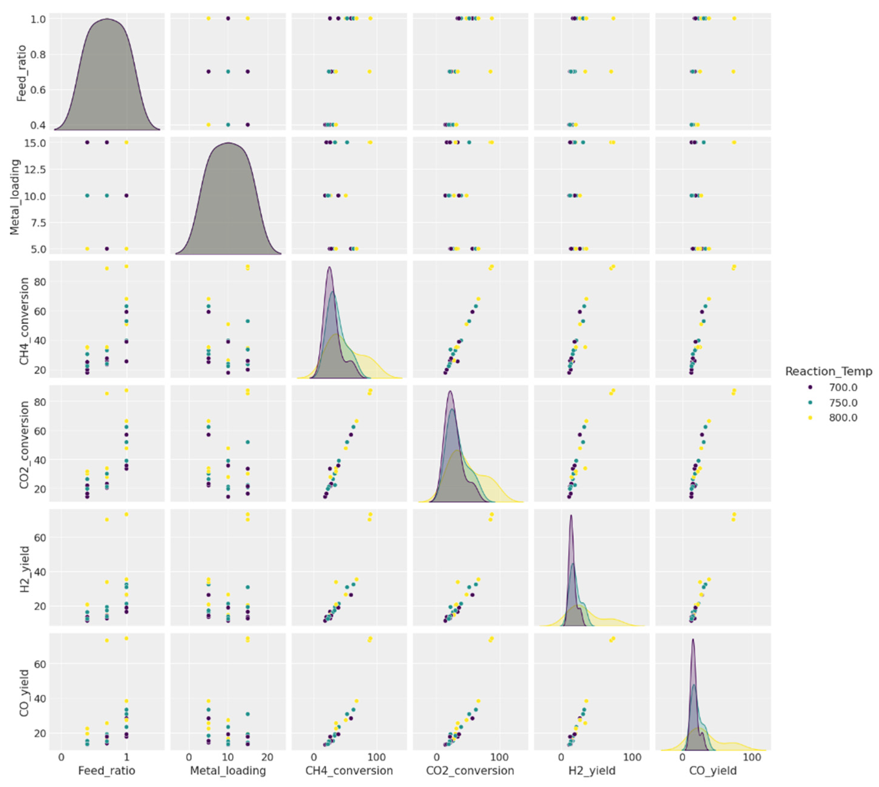
Pair plots (Figure 2) provide an overview of feature relationships and correlations. The sns.pairplot function was used to create scatter plots for all numerical variables, with colours representing reaction temperature (hue = ‘Reaction_Temp’) to highlight temperature-dependent trends. Diagonal Histograms Show variable distributions, revealing skewed trends in CH4 and CO2 conversions, indicating a higher frequency of lower conversion values.
Bivariate Relationships: CH4 and CO2 conversions exhibit a strong positive correlation, indicating that they are influenced by similar reaction conditions. Likewise, H2 and CO yields are positively correlated, suggesting that these products are generated through concurrent pathways. Analysis of feed ratio versus conversion reveals that higher reaction temperatures—represented by green and yellow data points—are associated with increased CH4 and CO2 conversion rates, particularly at elevated feed ratios. Additionally, both increased metal loading and higher temperatures contribute to improved conversion efficiency. The presence of distinct clusters in feed ratio and metal loading data further suggests categorical influences, likely reflecting specific experimental setups or catalyst formulations.
Colour Distribution and Temperature Trends: The distribution of data points by colour reveals clear temperature-dependent trends in DRM performance. Purple and blue points, which correspond to lower reaction temperatures (~700 °C), tend to cluster around lower CH4 and CO2 conversion values. In contrast, green and yellow point indicative of higher temperatures (~800 °C) are associated with significantly higher conversion rates and syngas (H2 and CO) yields. These visual patterns underscore the critical role of temperature in enhancing reaction efficiency. Moreover, such insights are valuable for feature selection and model training, reinforcing key trends that can improve the predictive accuracy of machine learning models.

3. Results and Discussion

This section presents a comprehensive evaluation of model performance, including correlation analysis, hyperparameter optimization via GridSearchCV, cross-validation outcomes, and regression metrics. Results are contextualized for practical applications in catalytic processes, particularly DRM.

3.1. Model Evaluation

The machine learning models were evaluated to identify the most effective algorithms for predicting DRM outputs. Model performance was assessed using the metrics outlined in Section 2.5, with a focus on accuracy and generalizability across all four targets.
A range of 15 regression models was assessed to predict CH4 conversion, CO2 conversion, H2 yield, and CO yield. Models included linear (Ridge, Lasso), regularized (ElasticNet), ensemble (Random Forest, Gradient Boosting, XGBoost, CatBoost, LightGBM), and kernel-based methods (SVR, NuSVR, Kernel Ridge), along with neural networks (MLP Regressor) and Bayesian Ridge. Model selection considered the ability to handle non-linear relationships, multicollinearity, and interaction effects, particularly for key variables like Feed Ratio and Reaction Temperature:
  • Ensemble methods and neural networks captured complex patterns via multiple learners or layers.
  • Kernel methods (SVR, NuSVR) effectively modelled non-linearities via feature space transformations.
  • Regularized models (Ridge, Lasso, ElasticNet) addressed multicollinearity by penalizing large coefficients.
  • Bayesian Ridge introduced probabilistic regularization via priors.
Models like Random Forest, Gradient Boosting, and CatBoost also offer feature importance metrics. While feature ranking is outside this paper’s scope, it provides potential for future insights [28,29,30,31,32]. The following sections summarize the impacts of feature engineering, model comparisons, and multi-output prediction performance.

3.2. Correlation Analysis

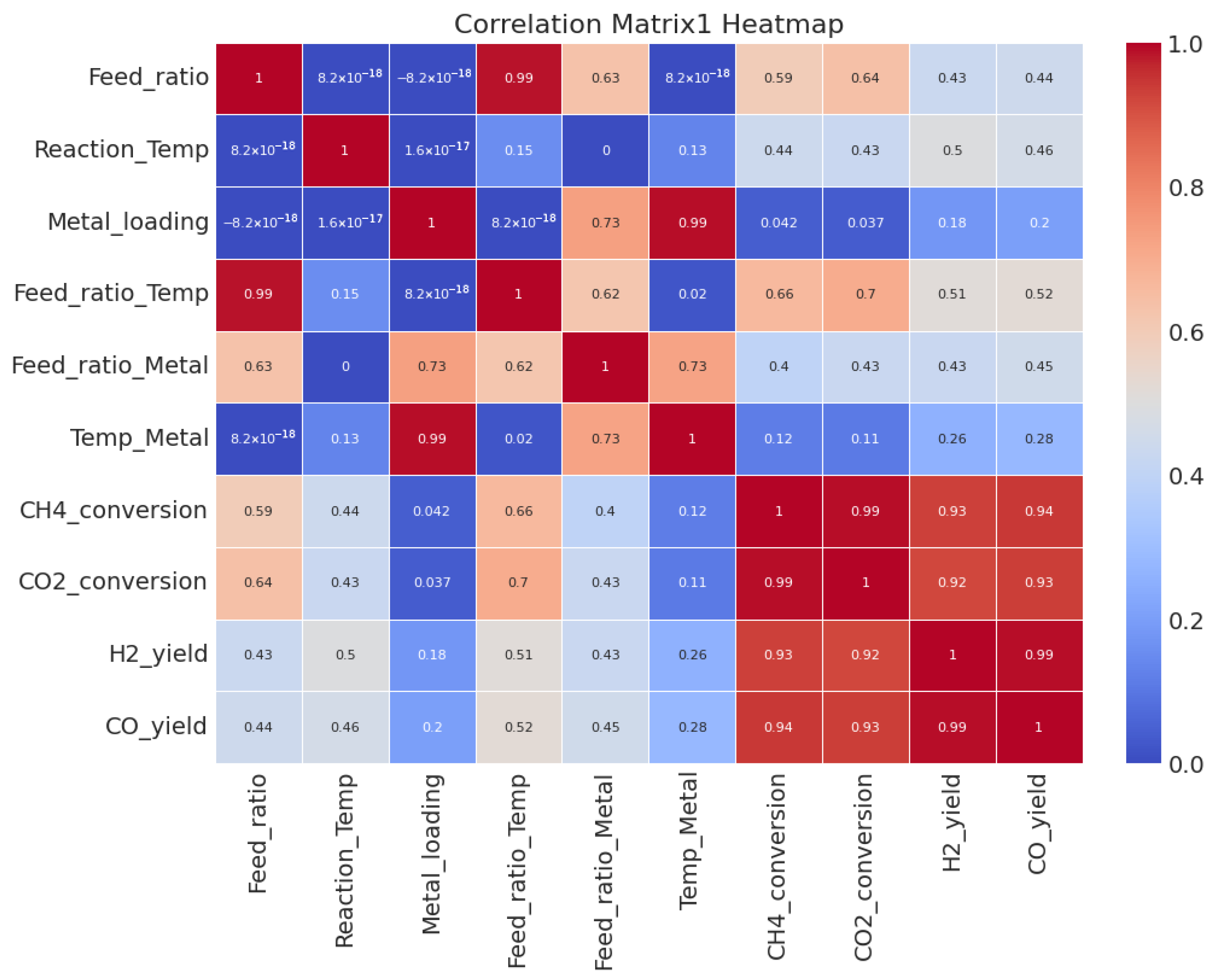
The correlation matrix presented in Figure 3 was generated using Pearson Correlation Coefficients (PCCs) to assess linear relationships among features and outputs. While some correlations—such as the positive association between reaction temperature and CH4 conversion—reflect well-known thermodynamic principles, the purpose of this analysis is primarily methodological. Specifically, it serves to:
(1) check data consistency and identify any anomalous trends prior to model development, and
(2) inform feature engineering by identifying variables and interactions with strong predictive influence.
Table 4 summarizes these correlations. Feed Ratio and Reaction Temperature exhibit the strongest positive correlations with CH4 and CO2 conversions (PCC = 0.59–0.70), confirming their dominant influence on DRM performance. Interaction terms, particularly Feed Ratio × Reaction Temperature, show even higher correlations (up to 0.70), justifying their inclusion as engineered features in the modeling pipeline. Although these findings align with established DRM trends, their primary role here is to enhance ML model interpretability and reduce the risk of introducing spurious relationships during feature generation.

3.3. Prediction Models and Hyperparameter Tuning

Fifteen regression models were evaluated using GridSearchCV with 3-fold and 5-fold cross-validation. Key hyperparameters were optimized for each model, balancing complexity and accuracy.

3.3.1. GridSearchCV Results

GridSearchCV provided robust hyperparameter tuning (Table A2 and Table A3Appendix C), enhancing model generalizability and reducing overfitting. Evaluation based on R2 and MSE for both train/test datasets indicated that CatBoost and Gradient Boosting consistently outperformed others.

3.3.2. Prediction Results

Fifteen regression models, including linear, regularized, ensemble, kernel-based, and neural network methods, were optimized using GridSearchCV and validated with LOOCV. Hyperparameters were tuned for each model to balance complexity and accuracy. Ensemble models (e.g., Random Forest, Gradient Boosting, CatBoost) demonstrated strong performance in capturing DRM non-linearities. Key parameters (e.g., estimators, depth, learning rate) were optimized for predictive efficiency. Models were assessed using R2 and MSE to identify optimal predictors for each output. The findings guide selection of models balancing interpretability and performance in catalytic process modelling.

3.3.3. Cross-Validation Comparison (CV = 3 vs. CV = 5)

Compared to 3-fold cross-validation, CV = 5 produced more stable performance estimates, particularly by reducing variance. Models such as Ridge, Lasso, and ElasticNet maintained consistent R2 values across folds, indicating reliability. In contrast, Extra Trees and LightGBM exhibited signs of overfitting, with high training R2 but poor generalization on test data—especially under CV = 3. CatBoost and Random Forest emerged as top performers, consistently achieving high test R2 across all folds, demonstrating strong generalizability.

3.3.4. Best Hyperparameters

Key hyperparameters identified through GridSearchCV are summarized in Table A3, highlighting the optimal configurations for each target variable. For CH4 conversion, CatBoost performed best on the original dataset with 50 iterations and a learning rate of 0.1, while Gradient Boosting on the polynomial-transformed data used a 0.01 learning rate and 200 estimators. CO2 conversion was optimized using CatBoost with 200 iterations and a 0.1 learning rate on the polynomial dataset, and Gradient Boosting with a 0.1 rate and 100 estimators. For H2 yield, Random Forest on the original dataset achieved strong results with 50 estimators and a maximum depth of 20, whereas CatBoost on the polynomial dataset used 200 iterations and a 0.1 learning rate. CO yield was best predicted using CatBoost (200 iterations, 0.1 rate) and Gradient Boosting (0.01 rate, 50 estimators) on the polynomial dataset. These hyperparameter settings effectively balanced model complexity and learning efficiency, leading to improved prediction accuracy across all targets.

3.3.5. Model Performance and Evaluation Metrics

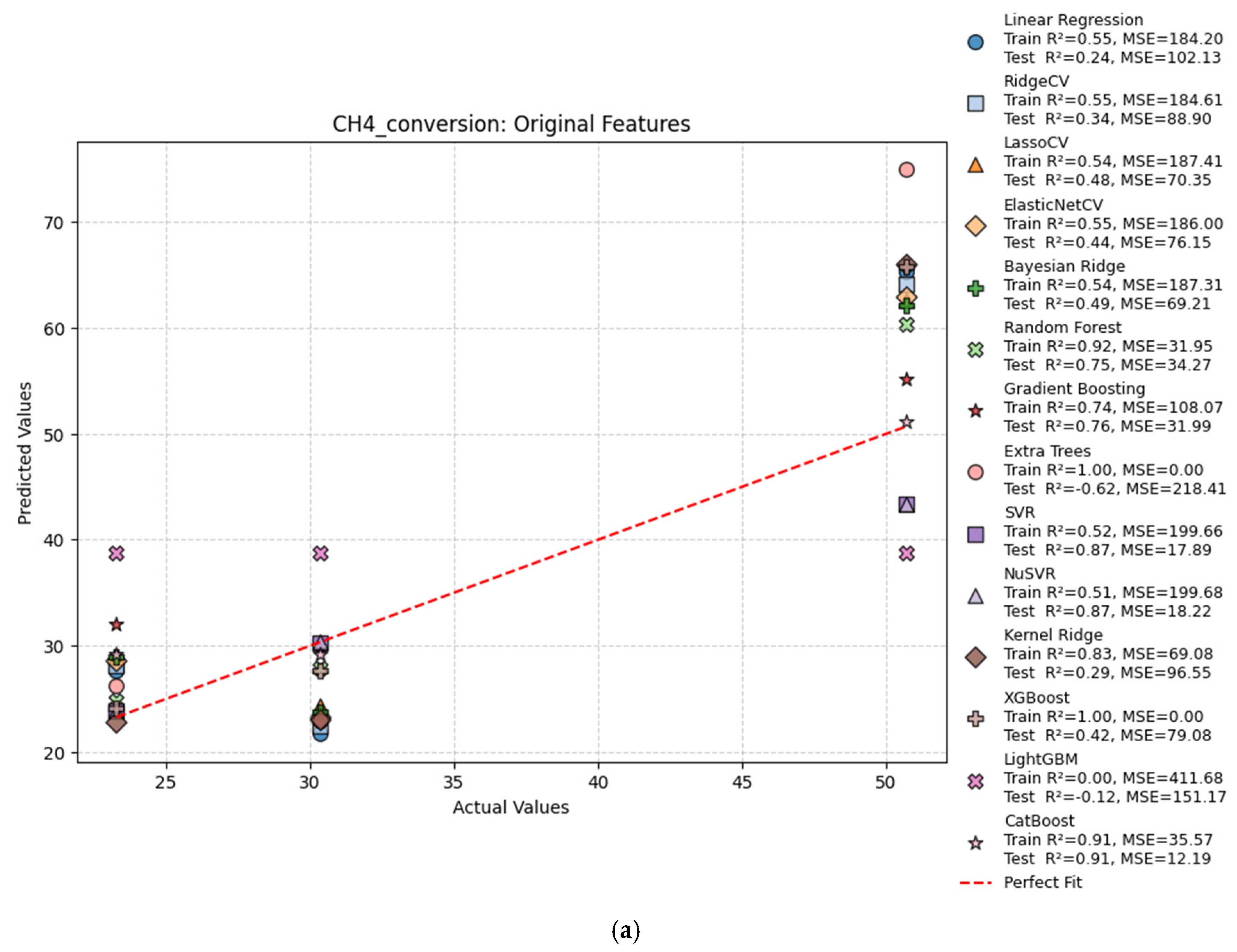
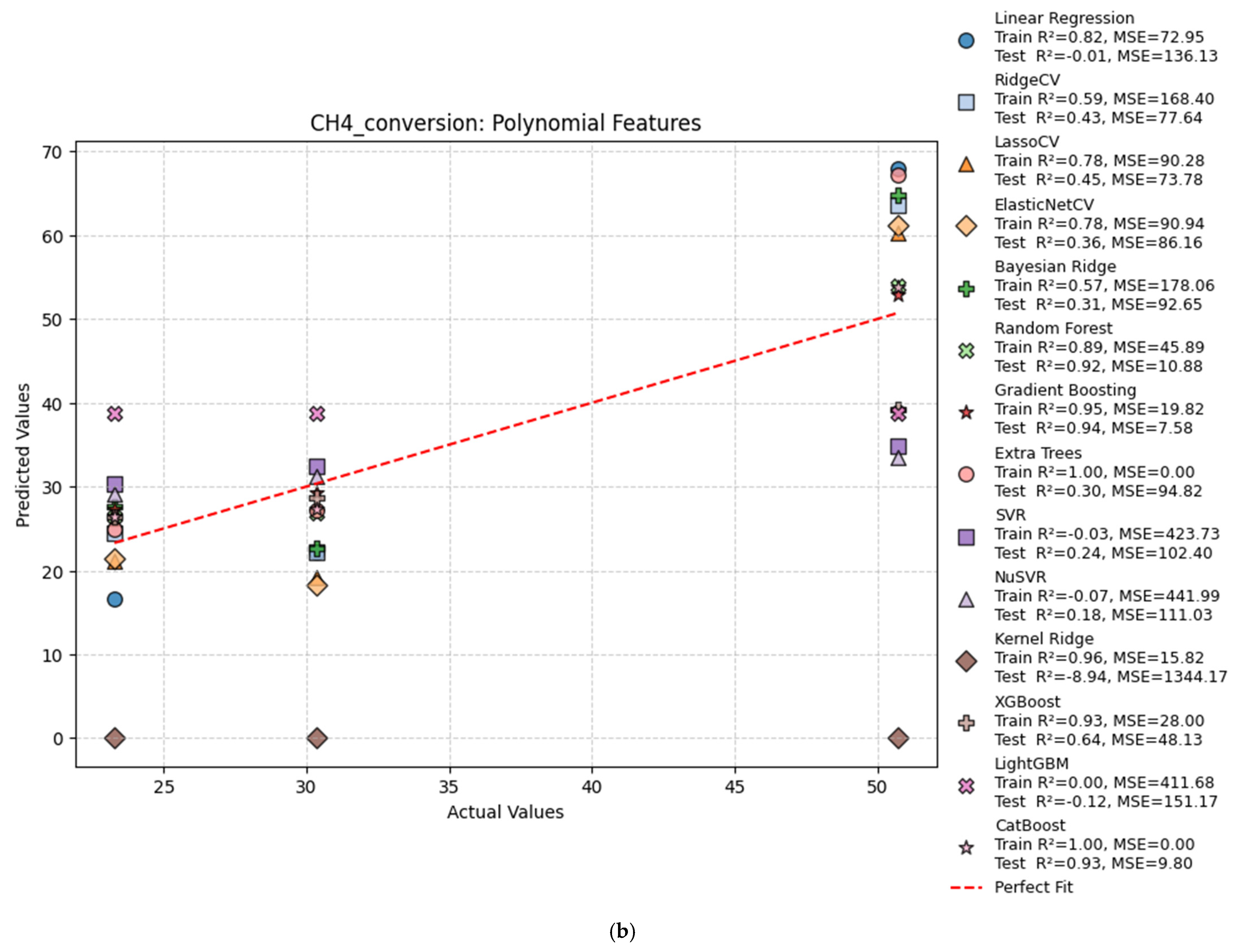
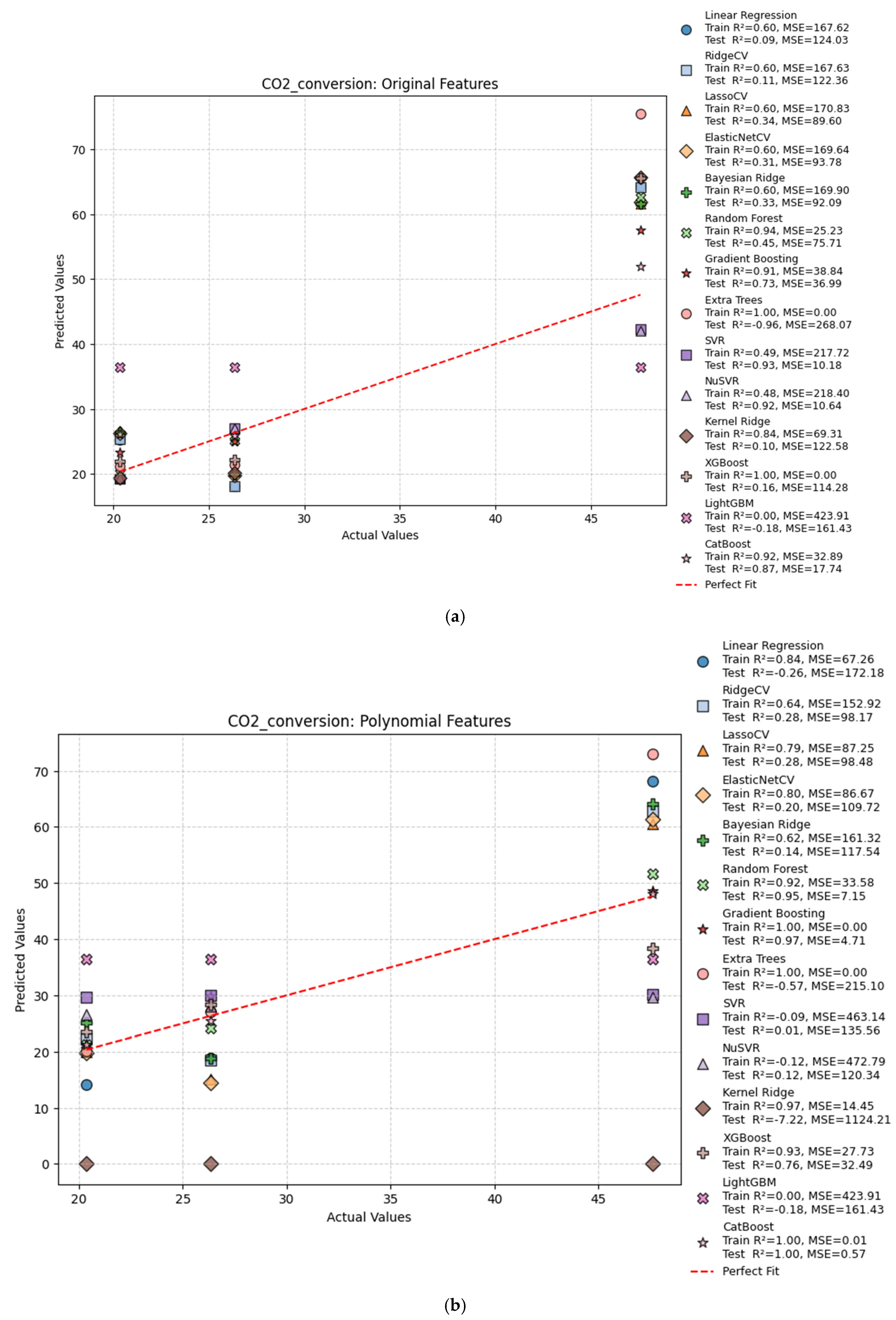
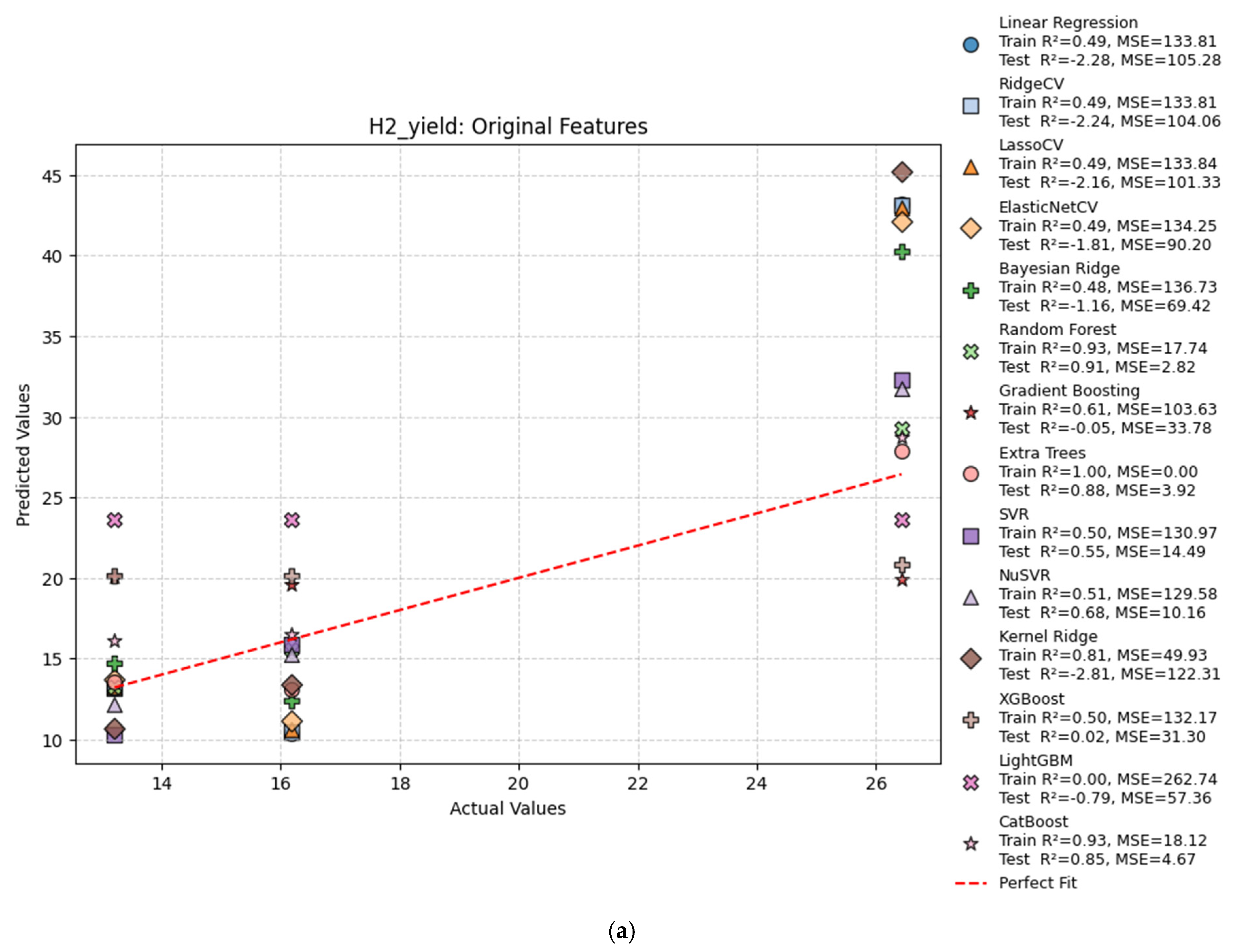
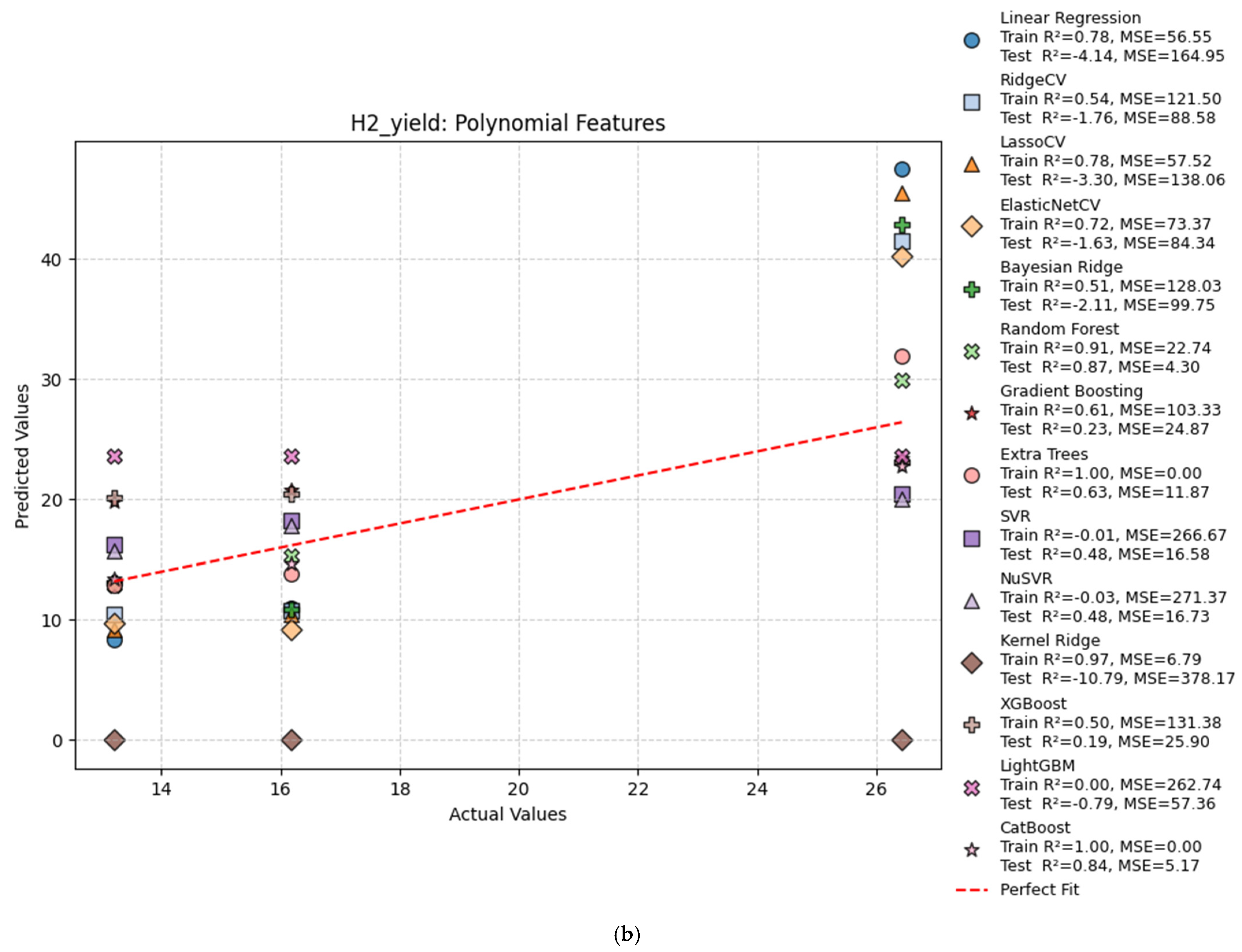
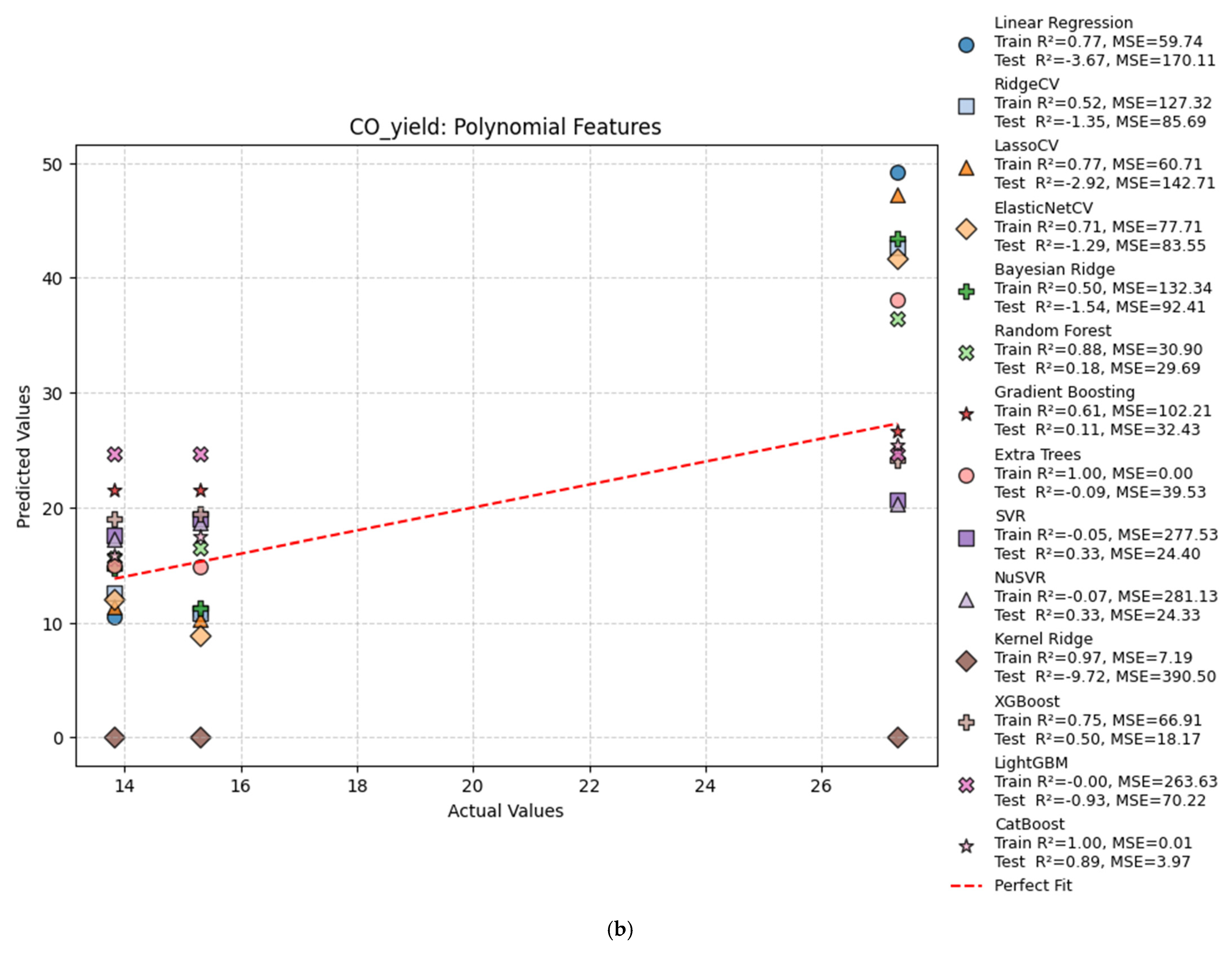
When evaluated on the test data, model performances varied considerably, as shown in Figure 4, Figure 5, Figure 6 and Figure 7. Model performance across the four DRM targets—CH4 conversion, CO2 conversion, H2 yield, and CO yield—is summarized in Table 5 and Figure 4, Figure 5, Figure 6 and Figure 7. Ensemble-based methods such as Random Forest and Gradient Boosting consistently produced predictions closest to the ideal line, reflecting their ability to capture nonlinear relationships in small datasets. In contrast, simpler linear models (e.g., Ridge, Lasso) exhibited greater scatter, particularly at the extremes of the observed range, indicating limitations in modeling complex interactions. Presenting the models together in these figures allows a direct, side-by-side visual comparison of predictive accuracy, highlighting both absolute performance and relative strengths across modeling approaches.
CatBoost on the original dataset achieved strong results for CH4 conversion (R2 = 0.91, MSE = 12.19), while Gradient Boosting with polynomial features performed slightly better (R2 = 0.94, MSE = 7.58). This is comparable to the results reported using ANN-MLP (Multi-layer Perceptron) with R2 = 0.96 and ANN-RBF (Radial Basis Function) with R2 = 0.83 [7]. For CO2 conversion, CatBoost with polynomial features delivered near-perfect accuracy (R2 = 1.00, MSE = 0.57), underscoring the value of feature transformation. This is comparable to ANN-MLP (R2 = 0.94) and ANN-RBF (R2 = 0.74) [7].
Random Forest excelled in predicting H2 yield (R2 = 0.88, MSE = 3.72), with CatBoost close behind (R2 = 0.84, MSE = 5.17). This is comparable to ANN-MLP (R2 = 0.97) and ANN-RBF (R2 = 0.92) [7]. In predicting CO yield, CatBoost again led (R2 = 0.89, MSE = 3.97), while Gradient Boosting on the original dataset underperformed (R2 = 0.21). This is comparable to ANN-MLP (R2 = 0.85) and ANN-RBF (R2 = 0.78) [7].
To ensure a fair comparison, we reimplemented the ANN-MLP and ANN-RBF models described by Hossain et al. [7] using the same dataset and a 70:30 train-test split. The resulting R2 values on the test set were substantially lower: for ANN-MLP, R2 = −0.99 (H2 yield), −1.03 (CO yield), −0.12 (CH4 conversion), and –0.08 (CO2 conversion); and for ANN-RBF, R2 = −2.91 (H2 yield), −3.47 (CO yield), −2.55 (CH4 conversion), and −2.26 (CO2 conversion). These results indicate poor generalization performance and suggest that the original study likely reported metrics based on training or full datasets.
Parity plots for the reimplemented ANN models (Figure 8) further illustrate the discrepancy between predicted and observed values on test data. These results demonstrate limited generalization performance in the earlier study compared to the models developed in this study.
In contrast, the models developed in this study—particularly CatBoost and Gradient Boosting—demonstrated consistently high R2 values across all targets on the test set, confirming their robustness and generalizability. In several cases, CatBoost predictions closely matched experimental values with minimal error. For example:
At 800 °C, CH4/CO2 = 1.0, Ni loading = 5 wt.%, experimental CH4 conversion was 67.93%, CatBoost predicted 68.00% (absolute error 0.07%).
At 800 °C, CH4/CO2 = 0.4, Ni loading = 15 wt.%, experimental CO2 conversion was 30.02%, CatBoost predicted 30.00% (absolute error 0.02%).
At 750 °C, CH4/CO2 = 1.0, Ni loading = 10 wt.%, experimental H2 yield was 21.11%, CatBoost predicted 21.00% (absolute error 0.11%).
At 750 °C, CH4/CO2 = 0.7, Ni loading = 10 wt.%, experimental CO yield was 15.06%, CatBoost predicted 15.00% (absolute error 0.06%).
These results highlight the importance of model selection, feature engineering, and rigorous validation. Overall, CatBoost consistently performed well across all targets due to its ability to capture complex interactions, while Gradient Boosting and Random Forest also showed strong generalizability. SVR and NuSVR captured non-linear trends but were prone to overfitting with polynomial features, emphasizing the need to align model complexity with data characteristics.

3.3.6. Leave-One-Out Cross-Validation (LOOCV) Results

Given the small dataset (n = 27), LOOCV was employed for a granular evaluation of model generalizability. Each sample was used once for validation, with the remainder for training. This maximized data utility and minimized bias in performance estimates (Table 6). Random Forest, Gradient Boosting, SVR, and CatBoost were chosen for LOOCV due to prior strong performance and ability to handle non-linear interactions efficiently.
To evaluate the influence of outliers on model performance, we conducted a sensitivity analysis by comparing predictions generated using the full dataset against those obtained after removing identified outliers. Outliers were detected based on outliers were identified using the Interquartile Range (IQR) method, which indicated data points with disproportionately high prediction errors.
Key Findings:
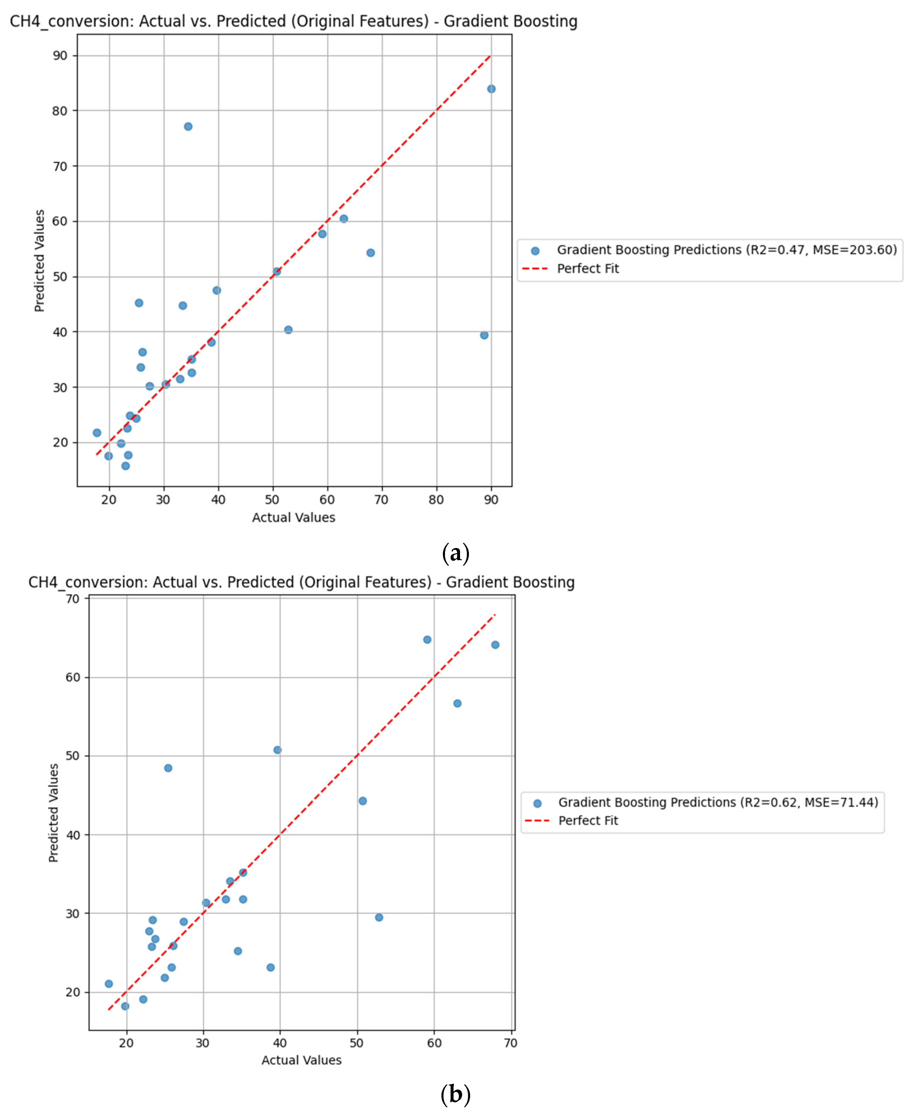
Figure 9 and Figure 10 illustrate the predicted versus actual values obtained from Leave-One-Out Cross-Validation (LOOCV) for Random Forest and Gradient Boosting models, respectively. Subfigures (a) show model performance on the original dataset including all samples, while subfigures (b) depict the results after removing the outliers.
Outlier removal significantly improved model accuracy, as seen in the Random Forest model for CH4 conversion, where R2 increased from 0.39 to 0.68 (Figure 9a,b and Figure 10a,b), highlighting the importance of data quality. Removal of outliers improved the alignment between predicted and actual values, as seen by tighter clustering around the ideal y = x line, particularly in the Gradient Boosting model (Figure 10b). CatBoost and Gradient Boosting maintained high R2 values even in the presence of outliers, demonstrating their robustness. This comparative analysis demonstrates that outlier removal is useful for understanding model sensitivity but was not used as a standard preprocessing step. All primary modelling conclusions were based on the full dataset to maintain data integrity and avoid bias. Polynomial feature transformations generally enhanced model performance, particularly for CatBoost and Gradient Boosting; however, SVR and NuSVR exhibited overfitting when such features were introduced, indicating sensitivity to model complexity.
Advantages of LOOCV:
Advantages of LOOCV include Lower Bias: Almost all data used for training in each iteration and High Sensitivity: Particularly valuable for small datasets, providing detailed performance estimates.
Challenges of LOOCV:
Challenges of LOOCV include Higher Variance: Results may vary due to model sensitivity to minor data changes and Computational Cost: Manageable in this study due to small sample size.
Comparison with GridSearchCV:
While GridSearchCV optimized hyperparameters using CV = 3/5, LOOCV offered detailed model validation. Both approaches together confirmed CatBoost, Gradient Boosting, and Random Forest as optimal for DRM predictions.
Bias-Variance Trade-Off:
Model performance revealed classic bias-variance trade-offs. Models with high variance, such as SVR with polynomial features, tended to overfit the training data, resulting in poor generalization and reduced accuracy on test sets. In contrast, low-bias models like linear regressors demonstrated reasonable accuracy during training but lacked the flexibility to capture the complex, non-linear patterns present in the data. These findings emphasize the importance of balancing model complexity to achieve optimal generalization performance.
To summarise, LOOCV reinforced model selection insights, emphasizing the value of CatBoost and Gradient Boosting for reliable DRM outcome prediction. These models, combined with appropriate feature engineering, offer robust and accurate predictions suitable for real-world applications.

3.3.7. CatBoost Hyperparameter R2 Analysis

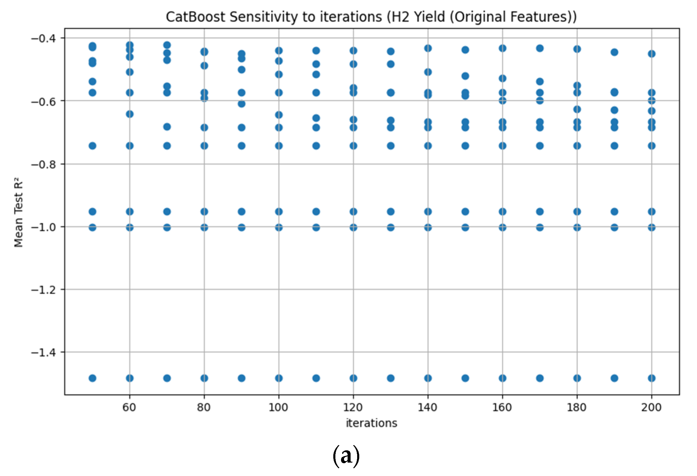
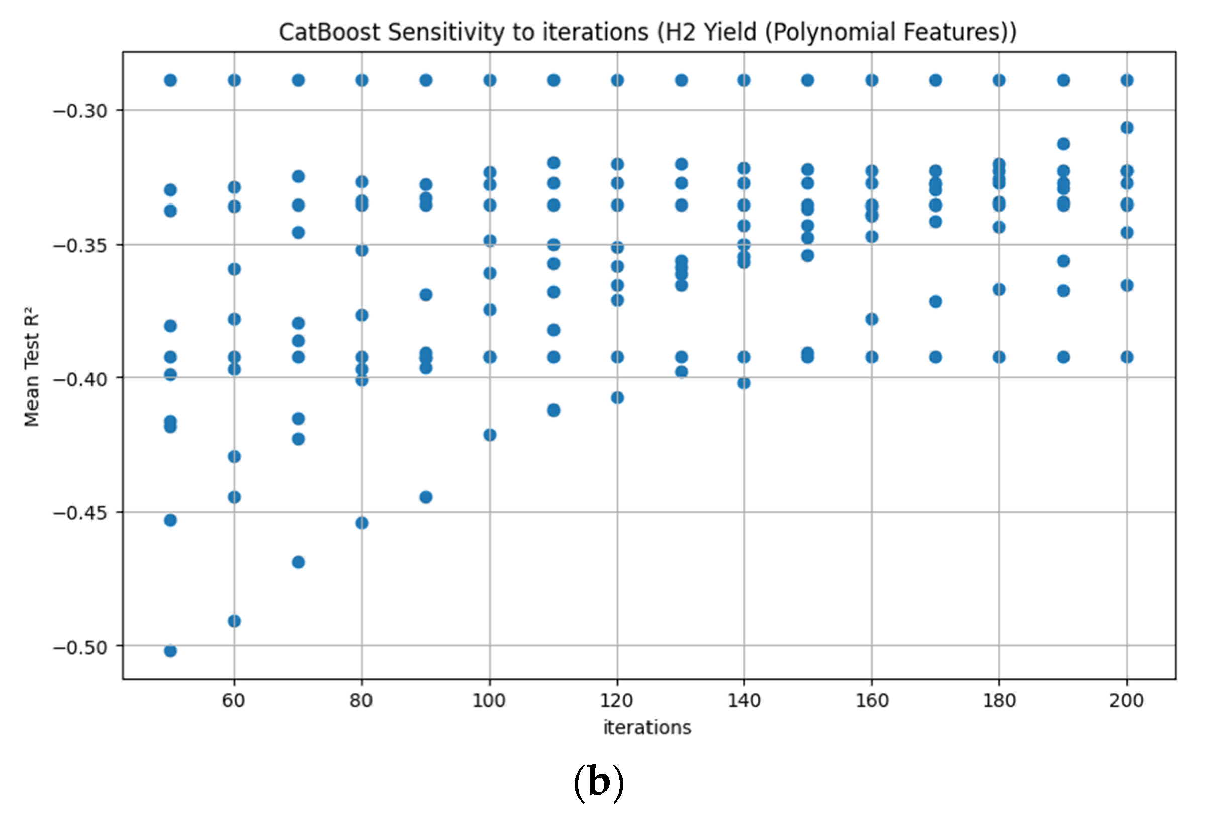
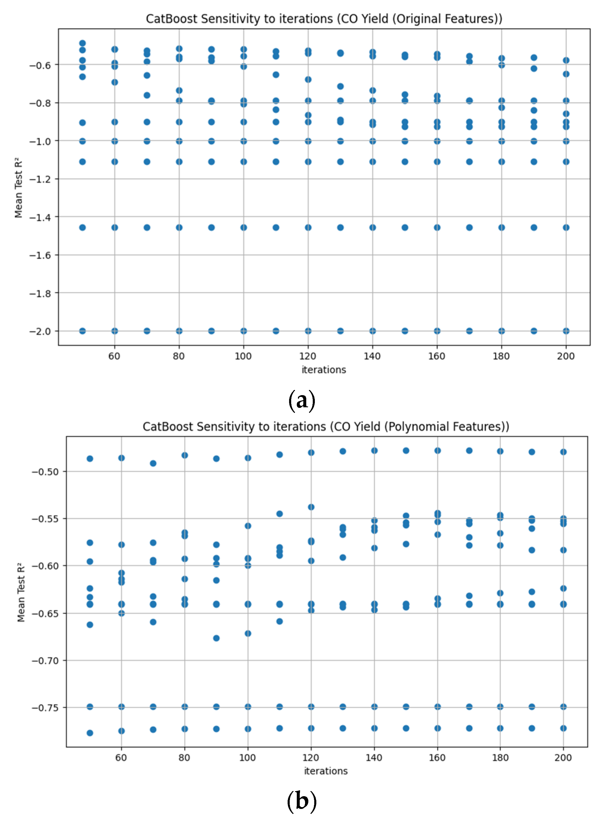
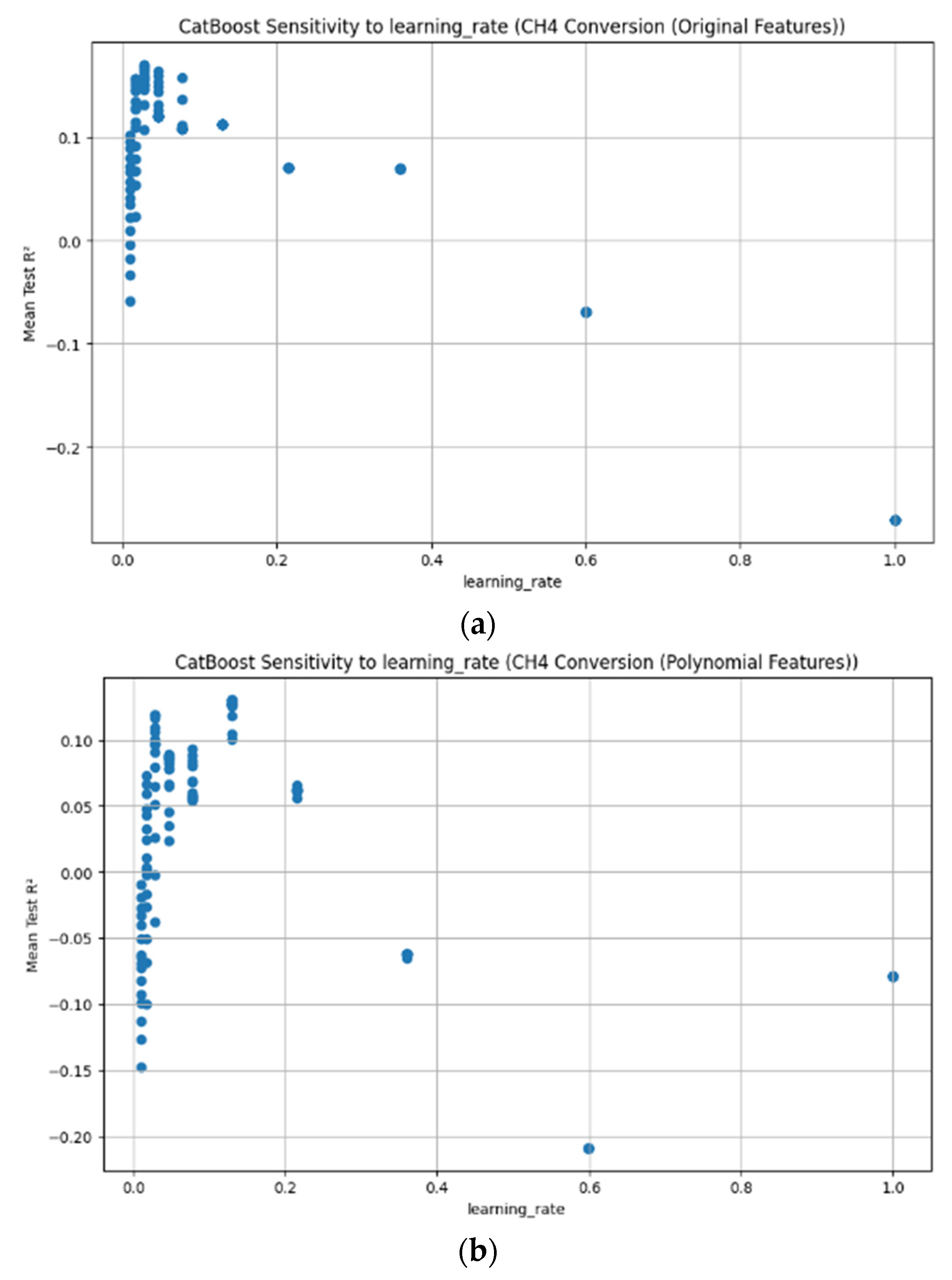
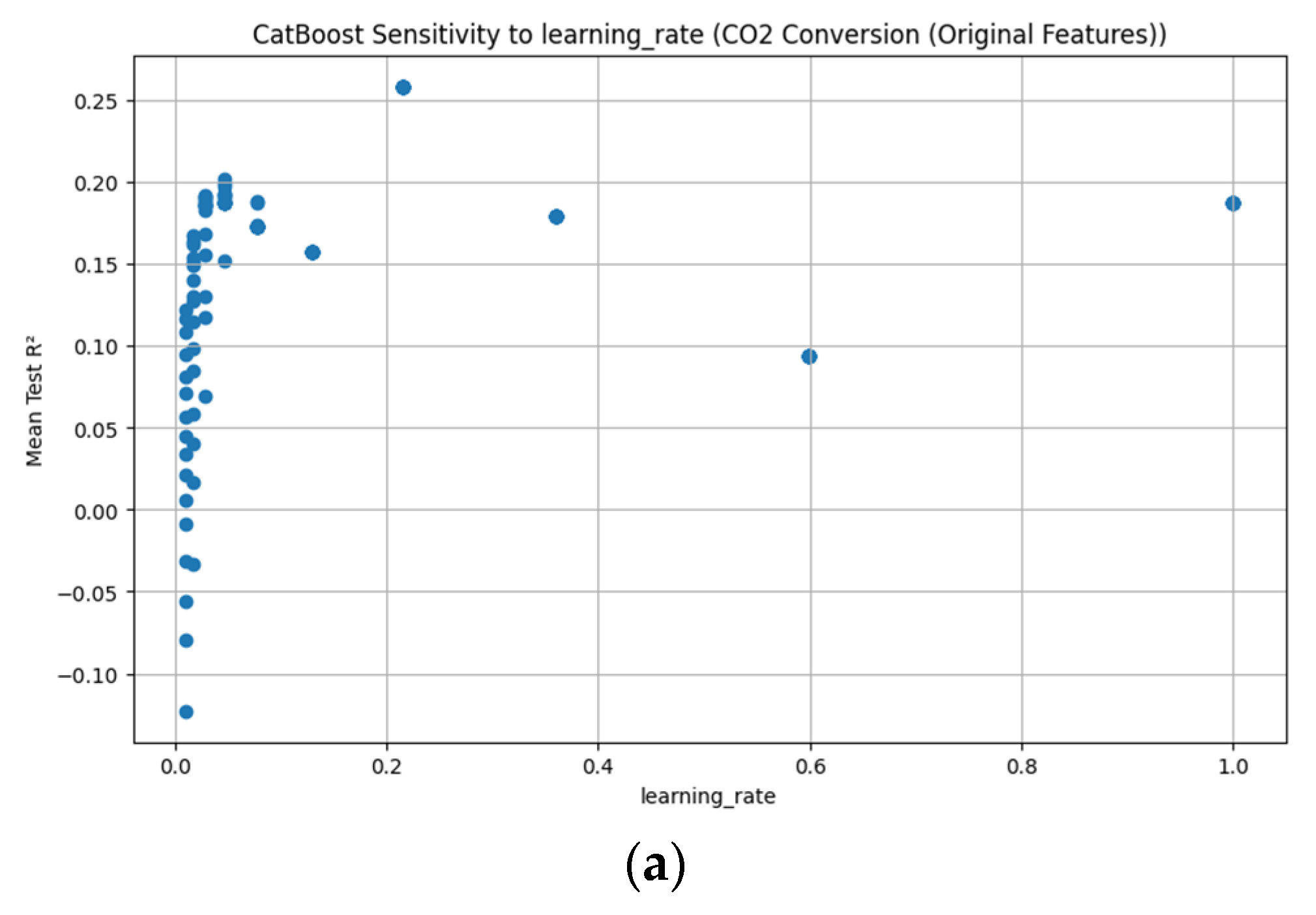
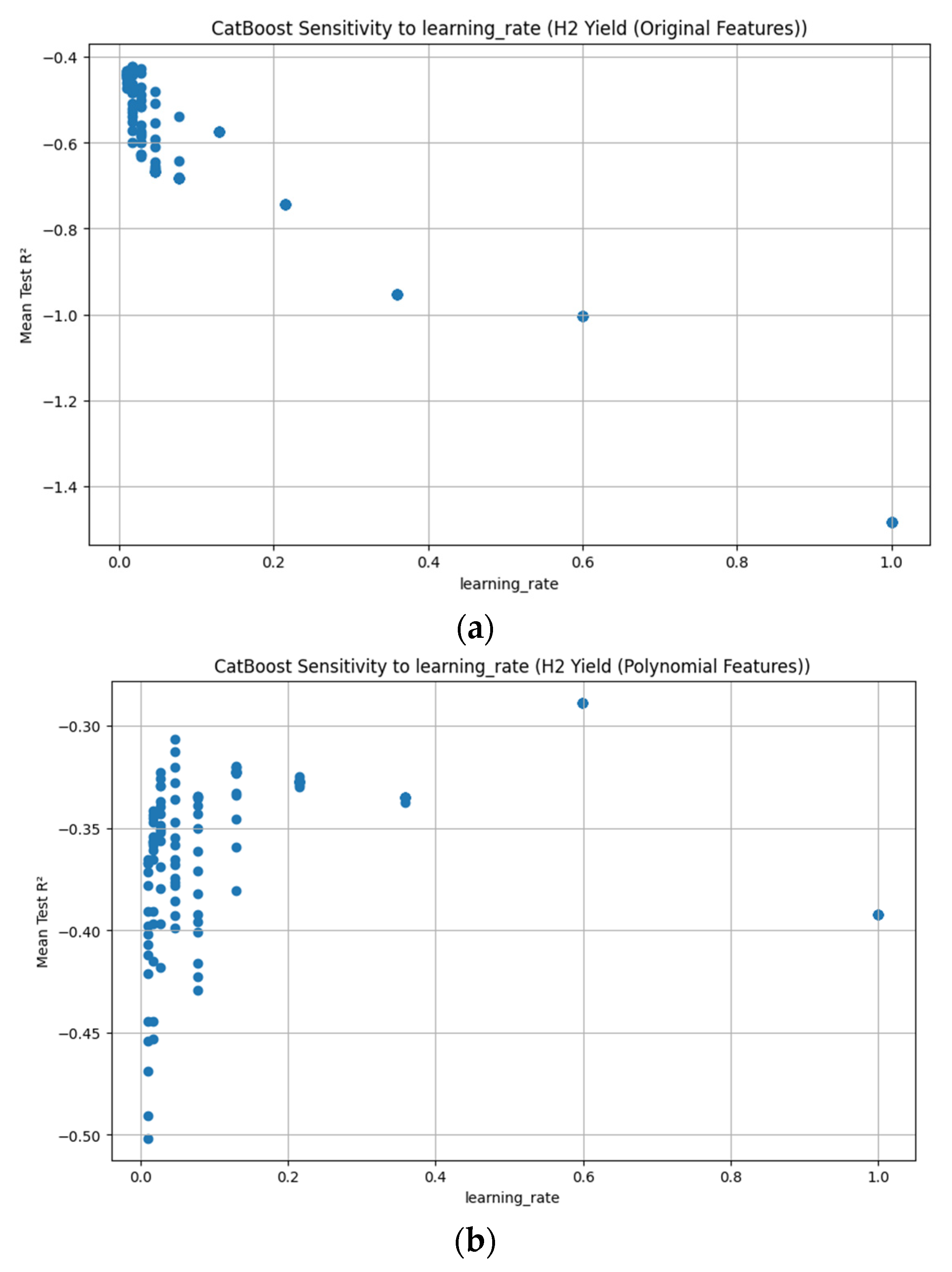
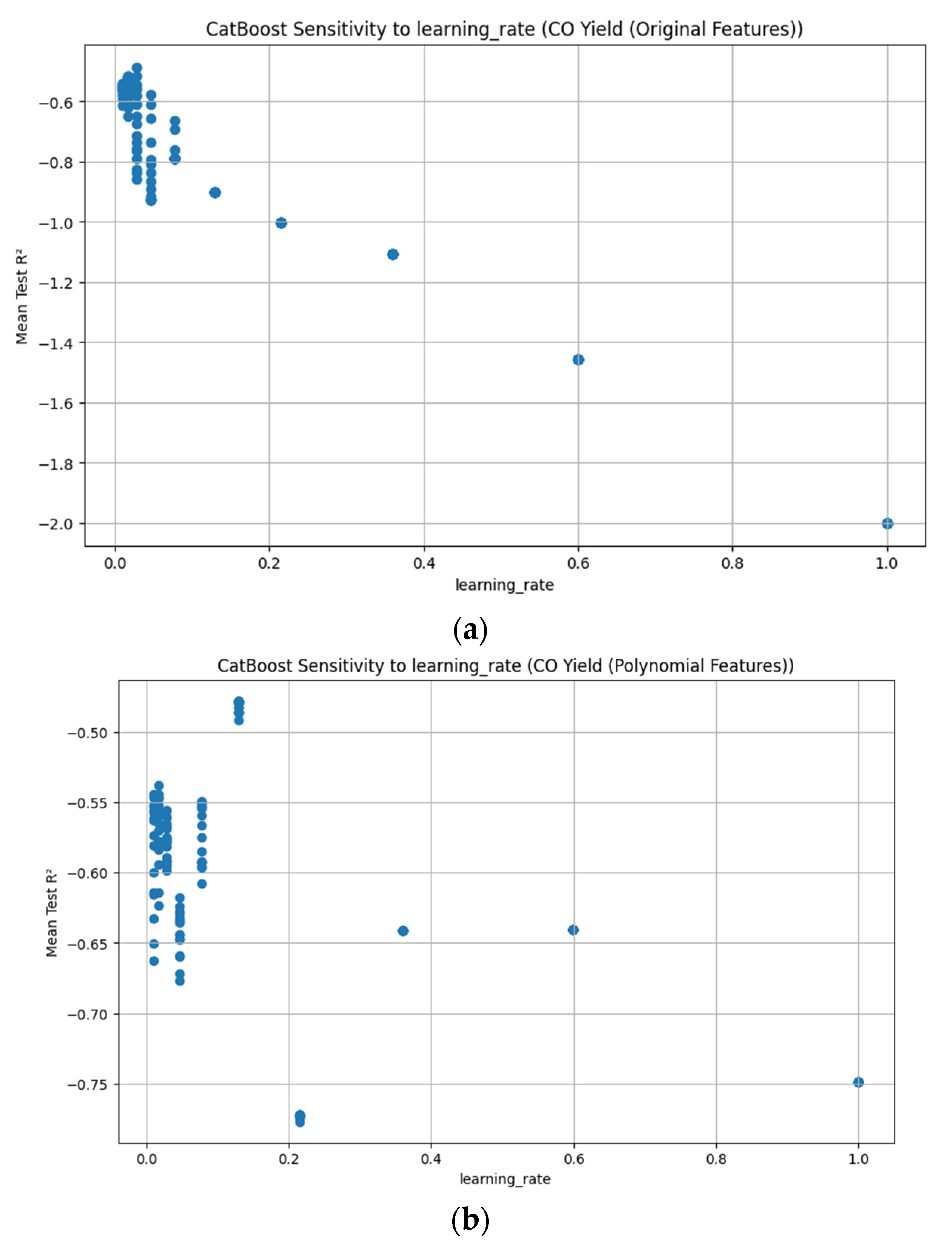
CatBoost exhibits robust performance, effectively managing complex data relationships, which results in high test R2 values. Its built-in regularization techniques mitigate overfitting, promoting strong generalization to unseen data. Hyperparameter interactions, such as between iterations and learning rate, contribute synergistically to performance improvement when optimally combined. (Figure A1, Figure A2, Figure A3, Figure A4, Figure A5, Figure A6, Figure A7 and Figure A8Appendix D) Illustrate the sensitivity of Mean Test R2 to these hyperparameter interactions for both original and polynomial features.
Key Insights:
Model performance was significantly influenced by the interaction of key hyperparameters, particularly the combination of iterations and learning rate. Even when individual contributions appeared modest, their optimal pairing led to substantial performance gains. CatBoost demonstrated a strong ability to capture intricate feature interactions, especially when polynomial features were included, further enhancing predictive accuracy. The relationship between the number of iterations and Mean Test R2 was notably non-linear, with performance peaking and then plateauing or declining—an indication of overfitting beyond a certain threshold. For H2 and CO yield, the optimal number of iterations was observed around 160, after which model performance began to deteriorate. Additionally, the learning rate played a critical role, with values between 0 and 0.2 yielding the most stable and reliable results across different iteration counts. In summary, CatBoost’s high-test R2 arises from the interplay of multiple hyperparameters and its inherent strengths. Proper hyperparameter tuning is critical to avoid overfitting and achieve optimal results.

3.3.8. Evaluation of Output Predictions Based on MAE and RMSE

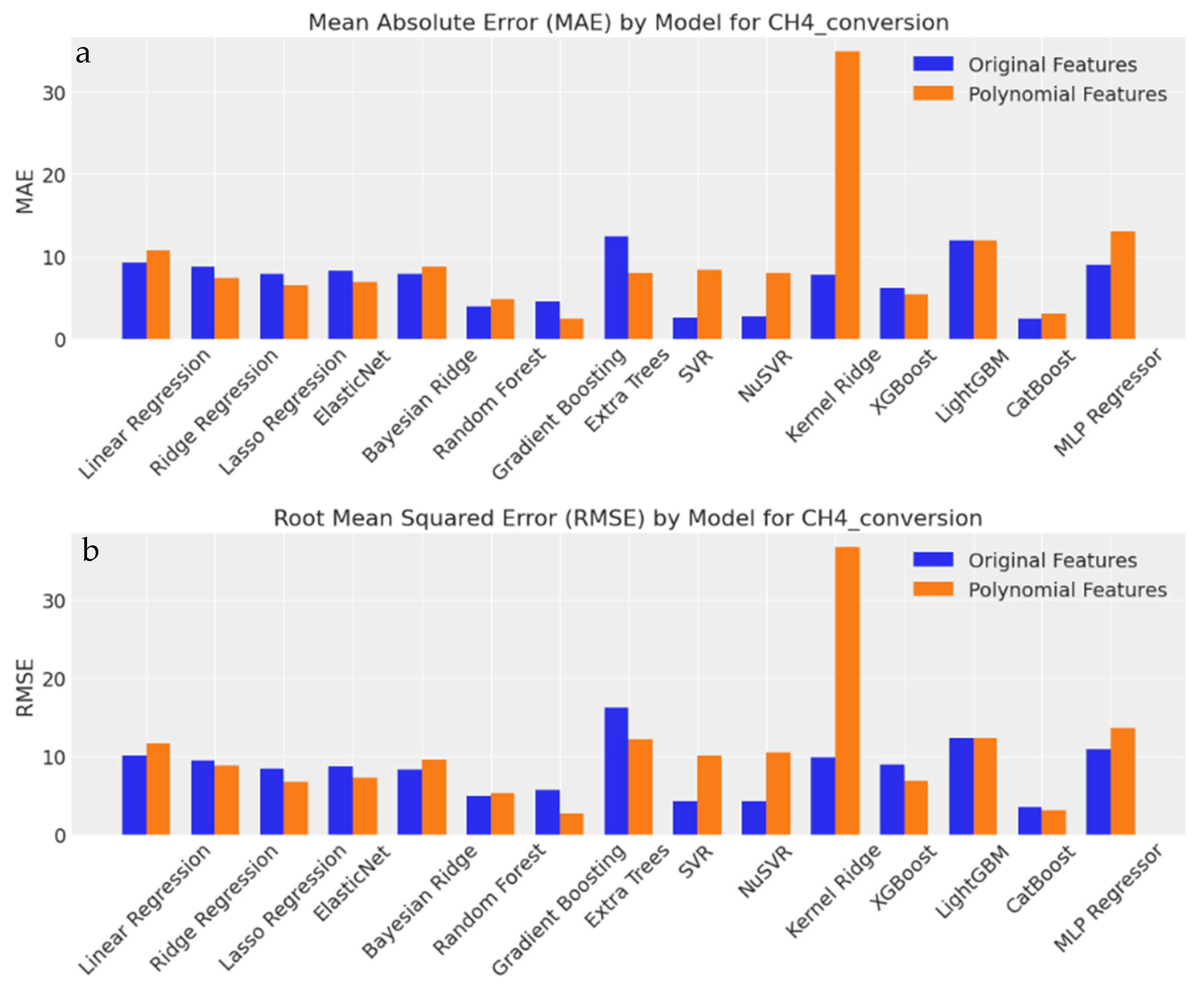
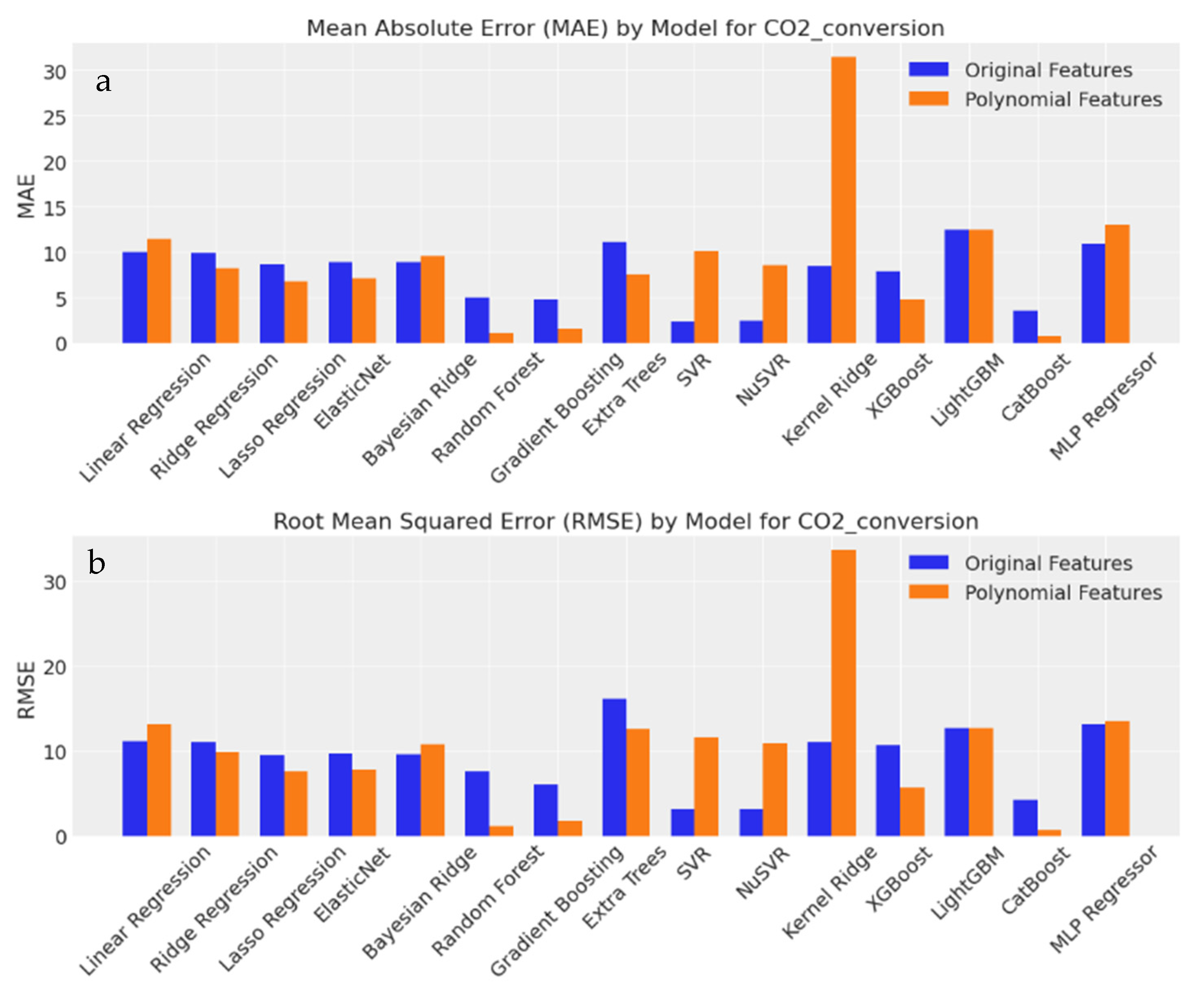
Figure 11, Figure 12, Figure 13 and Figure 14 display MAE and RMSE values for predicting CH4 Conversion, CO2 Conversion, H2 Yield, and CO Yield. These values align with trends in MSE and R2, supporting the reliability of model evaluations.
CH4 Conversion: Linear Regression: MAE = 9.20, RMSE = 10.11 (Original), MAE = 10.69, RMSE = 11.67 (Polynomial). Random Forest: MAE = 5.57, RMSE = 7.31 (Original), MAE = 3.17, RMSE = 3.30 (Polynomial). CatBoost: MAE = 2.52, RMSE = 3.50 (Original), MAE = 3.13, RMSE = 3.13 (Polynomial).
CO2 Conversion: Similar patterns were observed, with Gradient Boosting and Random Forest showing considerable improvements with polynomial features, while Kernel Ridge and SVR deteriorated.
H2 Yield: Models like Random Forest and Extra Trees showed significant improvements with polynomial features, while others such as Bayesian Ridge and MLP Regressor showed mixed results. CatBoost performed consistently well without polynomial features.
CO Yield: Polynomial features benefited Random Forest and Gradient Boosting, while SVR, NuSVR, and Kernel Ridge saw adverse effects. Extra Trees and XGBoost showed moderate improvements.
To summarise, MAE and RMSE metrics confirm trends observed in R2 and MSE.
Non-linear models such as Random Forest and Gradient Boosting benefit from polynomial features, while linear models often show degraded performance. CatBoost and Gradient Boosting generally outperform other models across various metrics (MAE, RMSE, R2, and MSE), indicating strong predictive power and minimal error. LOOCV results further validate these models’ robustness.

4. Model Performance Metrics in DRM: Comparing CH4 and CO2 Conversions with H2 and CO Yields

Model performance metrics reveal that CH4 and CO2 conversions generally outperform H2 and CO yields in DRM reactions. This disparity arises from several factors. The primary DRM reactions involving CH4 and CO2 are well-characterized and more straightforward, resulting in consistent conversion outcomes [35]. Catalysts are typically optimized for these conversions, whereas H2 and CO yields are more susceptible to catalyst deactivation, which can reduce performance [36]. Additionally, the thermodynamic equilibrium of DRM favors CH4 and CO2 conversion at elevated temperatures, while H2 and CO yields are more sensitive to fluctuations in temperature and pressure [39]. Finally, the reaction rates for CH4 and CO2 conversion are inherently higher than those for secondary reactions producing H2 and CO, contributing to the observed differences in predictive accuracy.

5. Parametric Influence, Interactions, and Predictive Insight

Predictions from the top-performing CatBoost and Random Forest models consistently indicated that optimal syngas production—maximizing H2 and CO yields—occurs when the CH4/CO2 feed ratio is near 1.0 and the reaction temperature is between 780–820 °C. These ranges align with well-established DRM operating windows, where sufficient thermal energy sustains the endothermic reaction while maintaining catalyst stability.
Key Variables: Feature importance rankings consistently identified reaction temperature, feed ratio, and Ni metal loading as the dominant factors influencing conversions and yields. Temperature showed the greatest influence, followed by feed ratio and metal loading.
Optimal Ranges and Interactions: Ni loading between 2–4 wt.% was found to positively impact yields, particularly at moderate temperatures. Interaction analysis revealed synergistic effects between feed ratio and temperature, and between temperature and metal loading. For example, slightly lean methane feeds (<1.0) can boost CO2 conversion at the expense of CH4 conversion, indicating potential trade-offs depending on desired syngas composition.
Practical Implications: These predictive insights enable rapid screening of promising conditions, allowing experimental efforts to focus on the most effective temperature–feed ratio–loading combinations. This approach is particularly useful in small-data scenarios, providing a data-efficient surrogate for guiding DRM experimentation.
Limitations: The trends reported here are derived from a dataset of 27 points for a single Ni/CaFe2O4 catalyst system. While consistent with DRM thermodynamics and literature trends, experimental validation across a wider range of catalysts and conditions is required to generalize these findings.
By translating model outputs into actionable operational guidance, this section bridges machine learning predictions with practical DRM process development.
Based on predictions from CatBoost and Random Forest models, optimal syngas production—defined by maximized H2 and CO yields—was consistently observed when the Feed Ratio approached 1.0 and Reaction Temperature ranged between 780–820 °C. These conditions align with well-established operating windows for dry reforming, where sufficient thermal energy sustains endothermic reforming while preserving catalyst stability. Although visual contour plots are not included in this version, the inferred response trends provide actionable insight into high-performance DRM regimes. However, based on predictions from CatBoost and Random Forest models, we observed that syngas production—defined here by higher H2 and CO yields—was consistently maximized when the Feed Ratio approached 1.0 and Reaction Temperature ranged between 780–820 °C. These conditions align with known optimal windows for dry reforming, where sufficient thermal energy drives endothermic reforming while maintaining catalytic stability. While we reserve detailed graphical visualizations for future or companion study, this quantitative inference provides actionable insight into high-performance DRM settings.
Additionally, interaction terms, particularly Feed Ratio × Reaction Temperature, correlated strongly with output variables (up to 0.70), underscoring synergistic effects between operating conditions. The outputs themselves were highly correlated (0.92–0.99), suggesting concurrent production trends and highlighting the potential for process-wide optimization strategies, indicating that DRM performance is primarily driven by thermal and compositional factors. These results align with previous studies highlighting DRM’s sensitivity to temperature and reactant ratios. Although, separate models were trained for multi-output and parallel single-output, they shared a unified preprocessing and feature engineering pipeline, enabling a multi-output learning framework through systematic coordination. This pragmatic structure reflects how multi-output modelling can be implemented in data-scarce environments without explicit multi-target regressors.
Use of Reinforcement Learning (RL) for multi-objective optimization in chemical processes derive optimal control policies by interacting with simulated environments or digital twins [40,41]. While RL excels in adaptive process control, this study takes a complementary approach by employing supervised learning to develop accurate predictive models for CH4 and CO2 conversions and H2 and CO yields based on experimental data. This predictive framework can serve as a data-efficient surrogate model, offering high-fidelity predictions for RL agents or control optimization algorithms in DRM.
To strengthen model interpretability, especially in the context of polynomial transformations, the study ensured that second-order terms were physically grounded (e.g., Feed Ratio × Temperature reflecting synergistic kinetic effects). The feature transformation pipeline details the interaction terms used and their chemical rationale. For example, the interaction between metal loading and temperature maps onto observed trends in catalyst stability, while Feed Ratio × Temperature captures known dependencies in DRM kinetics and equilibrium. This focus on feature engineering represents a central novelty of this study, particularly given the limited dataset.
Regarding model robustness, the Leave-One-Out Cross-Validation (LOOCV) and GridSearchCV for hyperparameter tuning help balance variance and bias in performance estimates. While LOOCV has inherent high variance, its thoroughness is valuable in small-data settings, and the use of additional test splits ensures that model overfitting is continuously monitored. Similar ML studies using small experimental datasets are reported [42].

6. Novelty and Impact

This study introduces several novel contributions to DRM research. Unlike conventional approaches that focus on single-output predictions, we employ multi-output regression models to simultaneously forecast CH4 conversion, CO2 conversion, H2 yield, and CO yield, enabling process-wide optimization. A comprehensive evaluation of fifteen machine learning models—including linear, ensemble, and Bayesian regressors—was conducted to identify the most accurate predictive framework. Feature transformations, such as polynomial expansions and interaction terms, along with outlier handling, significantly improved model accuracy and interpretability. Outlier analysis further refined model reliability by reducing predictive variance and revealing hidden inconsistencies in the experimental data. Importantly, the study supports low-carbon hydrogen production and contributes to carbon-neutral energy systems, aligning with Sustainable Development Goals 7 and 13. Overall, the findings offer actionable insights for optimizing DRM reactions in industrial settings and provide a robust framework for model selection and process enhancement.

7. Limitations and Future Work

While this study demonstrates the feasibility of using machine learning models for multi-output prediction in DRM, a few limitations remain. First, the dataset comprises only 27 samples from a single catalyst, which constrains model complexity, limits generalizability, and prevents the inclusion of catalyst property parameters known to influence reaction performance. Though LOOCV and GridSearchCV mitigate overfitting, the absence of catalyst descriptors (e.g., surface area, pore size, metal dispersion, chemical composition) represents a key restriction. Future work will focus on expanding the dataset with additional catalysts and their corresponding physicochemical properties, obtained through experimental runs or high-fidelity simulations, enabling integration of these descriptors as predictors. While polynomial feature transformations improved model accuracy, they may introduce interpretability challenges. Although the study emphasizes supervised regression, reinforcement learning and hybrid ML–reaction modelling strategies could further enhance process control and optimization under dynamic conditions.

8. Conclusions

This study demonstrates the effectiveness of various regression models in predicting DRM outcomes. CatBoost and Gradient Boosting consistently performed well, especially with polynomial features. CatBoost’s ability to manage both categorical and numerical data while preventing overfitting was a key strength, while Gradient Boosting’s sequential learning approach also yielded strong results. Random Forest showed robust performance, particularly for H2 Yield and CO2 Conversion. SVR and NuSVR effectively captured non-linear relationships but required careful tuning, especially with polynomial features. The study also highlighted the importance of cross-validation techniques, such as LOOCV, for small datasets. By evaluating multiple models and performing detailed outlier analysis, the study provides a comprehensive understanding of predictive modelling for DRM, with practical applications in optimizing reaction parameters for enhanced performance.

Author Contributions

Conceptualization, S.D.; methodology, S.D., J.S.T. and M.K.M.; software, S.D., J.S.T. and M.K.M.; validation, S.D.; formal analysis, S.D.; investigation, S.D., J.S.T. and M.K.M.; resources, S.D., J.S.T. and M.K.M.; data curation, S.D.; writing—original draft preparation, S.D., J.S.T. and M.K.M.; writing—review and editing S.D., J.S.T. and M.K.M.; visualization, S.D., J.S.T. and M.K.M.; supervision, S.D.; project administration, S.D.; All authors have read and agreed to the published version of the manuscript.

Funding

This research received no external funding.

Data Availability Statement

The data is included in the manuscript and the relevant citation [7] provided.

Conflicts of Interest

The authors declare no conflict of interest.

Appendix A

Table A1. Experimental data for the DRM reactions [7].
Expt. RunsInputsOutputs
Feed RatioReaction Temp (°C)Metal Loading (%)CH4 Conversion (%)CO2 Conversion (%)H2 Yield (%)CO Yield (%)
10.40800.0010.0022.9920.8413.2414.56
20.70800.0015.0088.6385.4170.3173.21
30.40750.0015.0023.4320.6813.5414.37
41.00700.005.0059.0856.9726.2228.32
51.00700.0015.0025.3833.5216.3517.70
61.00750.0010.0039.6038.9821.1123.32
70.40700.005.0025.0121.9613.2614.31
80.40800.0015.0034.4830.0220.3219.44
91.00800.0010.0050.7047.6026.4327.31
100.40750.005.0030.3426.3216.1715.31
110.70750.0015.0033.4522.2219.1519.15
120.70800.0010.0026.1127.7714.5416.59
130.40700.0010.0017.6914.1511.1213.09
140.70700.0010.0023.2720.3513.2113.83
150.40700.0015.0019.7816.3113.3713.37
160.70750.005.0032.8930.0217.1518.32
171.00750.005.0062.9362.3432.3633.31
181.00750.0015.0052.7651.8530.7730.77
190.70700.0015.0025.8221.3412.4517.70
200.70800.005.0035.0933.7733.7725.54
211.00700.0010.0038.7535.6818.7819.11
220.70700.005.0027.4623.1514.1415.32
230.70750.0010.0023.7821.1313.5615.06
241.00800.0015.0090.0487.6073.4274.43
250.40800.005.0035.1031.6220.6422.41
260.40750.0010.0022.1619.6012.2113.39
271.00800.005.0067.9366.3935.3638.31

Appendix B

The conversion rates of CH4 and CO2 and the yields of H2 and CO were calculated using the Equations (A1)–(A4):
C H 4 c o n v e r s i o n = F C H 4 i n F C H 4 o u t F C H 4 i n × 100
C O 2 c o n v e r s i o n = F C O 2 i n F C O 2 o u t F C O 2 i n × 100
H 2 y i e l d = F H 2 o u t 2 × F C H 4 i n × 100
C O y i e l d = F C O o u t F C O 2 i n + F C H 4 i n × 100
where F represents the molar flow rates of CO2, CH4, CO, and H2 at the reactor inlet and outlet [7].

Appendix C

Table A2. Model metrics for original features using Grid Search CV (for CV = 3 and CV = 5).
ModelMetricCV = 3, OriginalCV = 5, Original
LinearCH4_conversionTrain R2 = 0.55, Test R2 = 0.24Train R2 = 0.55, Test R2 = 0.24
CO2_conversionTrain R2 = 0.60, Test R2 = 0.09Train R2 = 0.60, Test R2 = 0.09
H2_yieldTrain R2 = 0.49, Test R2 = −2.28Train R2 = 0.49, Test R2 = −2.28
CO_yieldTrain R2 = 0.48, Test R2 = −1.68Train R2 = 0.48, Test R2 = −1.68
Ridge CH4_conversionTrain R2 = 0.55, Test R2 = 0.34Train R2 = 0.55, Test R2 = 0.34
CO2_conversionTrain R2 = 0.60, Test R2 = 0.21Train R2 = 0.60, Test R2 = 0.11
H2_yieldTrain R2 = 0.49, Test R2 = −2.28Train R2 = 0.49, Test R2 = −2.24
CO_yieldTrain R2 = 0.48, Test R2 = −1.65Train R2 = 0.48, Test R2 = −1.65
Lasso CH4_conversionTrain R2 = 0.54, Test R2 = 0.48Train R2 = 0.54, Test R2 = 0.48
CO2_conversionTrain R2 = 0.60, Test R2 = 0.34Train R2 = 0.60, Test R2 = 0.34
H2_yieldTrain R2 = 0.49, Test R2 = −2.16Train R2 = 0.49, Test R2 = −2.16
CO_yieldTrain R2 = 0.48, Test R2 = −1.59Train R2 = 0.48, Test R2 = −1.59
ElasticNetCH4_conversionTrain R2 = 0.55, Test R2 = 0.44Train R2 = 0.55, Test R2 = 0.44
CO2_conversionTrain R2 = 0.60, Test R2 = 0.24Train R2 = 0.60, Test R2 = 0.31
H2_yieldTrain R2 = 0.49, Test R2 = −1.81Train R2 = 0.49, Test R2 = −1.81
CO_yieldTrain R2 = 0.47, Test R2 = −1.31Train R2 = 0.47, Test R2 = −1.31
Bayesian RidgeCH4_conversionTrain R2 = 0.54, Test R2 = 0.49Train R2 = 0.54, Test R2 = 0.49
CO2_conversionTrain R2 = 0.60, Test R2 = 0.33Train R2 = 0.60, Test R2 = 0.33
H2_yieldTrain R2 = 0.48, Test R2 = −1.16Train R2 = 0.48, Test R2 = −1.16
CO_yieldTrain R2 = 0.46, Test R2 = −0.75Train R2 = 0.46, Test R2 = −0.75
Random ForestCH4_conversionTrain R2 = 0.93, Test R2 = 0.79Train R2 = 0.91, Test R2 = 0.76
CO2_conversionTrain R2 = 0.93, Test R2 = 0.77Train R2 = 0.94, Test R2 = 0.72
H2_yieldTrain R2 = 0.91, Test R2 = 0.69Train R2 = 0.93, Test R2 = 0.72
CO_yieldTrain R2 = 0.91, Test R2 = −0.22Train R2 = 0.92, Test R2 = 0.46
Gradient BoostingCH4_conversionTrain R2 = 0.50, Test R2 = 0.66Train R2 = 0.74, Test R2 = 0.76
CO2_conversionTrain R2 = 0.52, Test R2 = 0.70Train R2 = 0.91, Test R2 = 0.73
H2_yieldTrain R2 = 1.00, Test R2 = 0.61Train R2 = 0.61, Test R2 = −0.05
CO_yieldTrain R2 = 0.62, Test R2 = 0.21Train R2 = 0.62, Test R2 = 0.21
Extra TreesCH4_conversionTrain R2 = 1.00, Test R2 = −0.66Train R2 = 1.00, Test R2 = −0.87
CO2_conversionTrain R2 = 1.00, Test R2 = −1.04Train R2 = 1.00, Test R2 = −1.02
H2_yieldTrain R2 = 1.00, Test R2 = 0.44Train R2 = 1.00, Test R2 = 0.86
CO_yieldTrain R2 = 1.00, Test R2 = −0.03Train R2 = 1.00, Test R2 = 0.10
SVRCH4_conversionTrain R2 = 0.52, Test R2 = 0.87Train R2 = 0.52, Test R2 = 0.87
CO2_conversionTrain R2 = 0.49, Test R2 = 0.93Train R2 = 0.49, Test R2 = 0.93
H2_yieldTrain R2 = 0.50, Test R2 = 0.55Train R2 = 0.50, Test R2 = 0.55
CO_yieldTrain R2 = 0.43, Test R2 = 0.82Train R2 = 0.43, Test R2 = 0.82
NuSVRCH4_conversionTrain R2 = 0.57, Test R2 = 0.98Train R2 = 0.51, Test R2 = 0.87
CO2_conversionTrain R2 = 0.48, Test R2 = 0.92Train R2 = 0.48, Test R2 = 0.92
H2_yieldTrain R2 = 0.51, Test R2 = 0.68Train R2 = 0.51, Test R2 = 0.68
CO_yieldTrain R2 = 0.46, Test R2 = 0.76Train R2 = 0.46, Test R2 = 0.76
Kernel RidgeCH4_conversionTrain R2 = 0.83, Test R2 = 0.29Train R2 = 0.83, Test R2 = 0.29
CO2_conversionTrain R2 = 0.84, Test R2 = 0.10Train R2 = 0.84, Test R2 = 0.10
H2_yieldTrain R2 = 0.81, Test R2 = −2.81Train R2 = 0.81, Test R2 = −2.81
CO_yieldTrain R2 = 0.80, Test R2 = −2.49Train R2 = 0.80, Test R2 = −2.49
XGBoostCH4_conversionTrain R2 = 0.69, Test R2 = 0.65Train R2 = 1.00, Test R2 = 0.42
CO2_conversionTrain R2 = 1.00, Test R2 = 0.16Train R2 = 1.00, Test R2 = 0.16
H2_yieldTrain R2 = 1.00, Test R2 = 0.33Train R2 = 0.50, Test R2 = 0.02
CO_yieldTrain R2 = 1.00, Test R2 = 0.07Train R2 = 0.49, Test R2 = 0.17
LightGBMCH4_conversionTrain R2 = 0.00, Test R2 = −0.12Train R2 = 0.00, Test R2 = −0.12
CO2_conversionTrain R2 = 0.00, Test R2 = −0.18Train R2 = 0.00, Test R2 = −0.18
H2_yieldTrain R2 = 0.00, Test R2 = −0.79Train R2 = 0.00, Test R2 = −0.79
CO_yieldTrain R2 = −0.00, Test R2 = −0.93Train R2 = −0.00, Test R2 = −0.93
CatBoostCH4_conversionTrain R2 = 0.99, Test R2 = 0.91Train R2 = 0.91, Test R2 = 0.91
CO2_conversionTrain R2 = 0.92, Test R2 = 0.87Train R2 = 0.92, Test R2 = 0.87
H2_yieldTrain R2 = 1.00, Test R2 = 0.67Train R2 = 0.93, Test R2 = 0.85
CO_yieldTrain R2 = 1.00, Test R2 = 0.77Train R2 = 0.93, Test R2 = 0.79
MLP RegressorCH4_conversionTrain R2 = 0.98, Test R2 = 0.39Train R2 = 0.80, Test R2 = −0.12
CO2_conversionTrain R2 = 0.82, Test R2 = −0.16Train R2 = 0.82, Test R2 = −0.44
H2_yieldTrain R2 = 0.76, Test R2 = −4.79Train R2 = 0.76, Test R2 = −4.84
CO_yieldTrain R2 = 0.75, Test R2 = −4.03Train R2 = 0.75, Test R2 = −4.10
Table A3. Regression models, best parameters (for Grid Search).
CH4 Conversion
Feature TypeModelParameters
OriginalLinear Regression{}
OriginalRidge Regression{‘alphas’: 1.0}
OriginalLasso Regression{‘alphas’: [1.0 × 10⁻³, 1.0 × 10⁻², 1.0 × 10⁻¹, 1.0 × 100, 1.0 × 101, 1.0 × 10², 1.0 × 10³]}
OriginalElasticNet{‘alphas’: [1.0 × 10⁻³, 1.0 × 10⁻², 1.0 × 10⁻¹, 1.0 × 100, 1.0 × 101, 1.0 × 10², 1.0 × 10³], ‘l1_ratio’: 0.1}
OriginalBayesian Ridge{‘alpha_1’: 0.001, ‘alpha_2’: 1 × 10⁻⁶, ‘lambda_1’: 1 × 10⁻⁶, ‘lambda_2’: 0.001}
OriginalRandom Forest{‘max_depth’: None, ‘n_estimators’: 100}
OriginalGradient Boosting{‘learning_rate’: 0.01, ‘n_estimators’: 100}
OriginalExtra Trees{‘max_depth’: None, ‘n_estimators’: 100}
OriginalSVR{‘C’: 10, ‘gamma’: ‘scale’}
OriginalNuSVR{‘C’: 10, ‘nu’: 0.9}
OriginalKernel Ridge{‘alpha’: 0.1, ‘gamma’: 0.1}
OriginalXGBoost{‘learning_rate’: 1, ‘n_estimators’: 50}
OriginalLightGBM{‘learning_rate’: 0.01, ‘n_estimators’: 50}
OriginalCatBoost{‘iterations’: 50, ‘learning_rate’: 0.1}
OriginalMLP Regressor{‘activation’: ‘relu’, ‘alpha’: 0.01, ‘batch_size’: 32, ‘hidden_layer_sizes’: (100,), ‘solver’: ‘adam’}
PolyLinear Regression{}
PolyRidge Regression{‘alphas’: 1000.0}
PolyLasso Regression{‘alphas’: [1.0 × 10⁻³, 1.0 × 10⁻², 1.0 × 10⁻¹, 1.0 × 100, 1.0 × 101, 1.0 × 10², 1.0 × 10³]}
PolyElasticNet{‘alphas’: [1.0 × 10⁻³, 1.0 × 10⁻², 1.0 × 10⁻¹, 1.0 × 100, 1.0 × 101, 1.0 × 10², 1.0 × 10³], ‘l1_ratio’: 0.1}
PolyBayesian Ridge{‘alpha_1’: 0.001, ‘alpha_2’: 1 × 10⁻⁶, ‘lambda_1’: 1 × 10⁻⁶, ‘lambda_2’: 0.001}
PolyRandom Forest{‘max_depth’: 20, ‘n_estimators’: 100}
PolyGradient Boosting{‘learning_rate’: 0.01, ‘n_estimators’: 200}
PolyExtra Trees{‘max_depth’: None, ‘n_estimators’: 50}
PolySVR{‘C’: 10, ‘gamma’: ‘scale’}
PolyNuSVR{‘C’: 10, ‘nu’: 0.9}
PolyKernel Ridge{‘alpha’: 0.1, ‘gamma’: 0.1}
PolyXGBoost{‘learning_rate’: 0.01, ‘n_estimators’: 200}
PolyLightGBM{‘learning_rate’: 0.01, ‘n_estimators’: 50}
PolyCatBoost{‘iterations’: 200, ‘learning_rate’: 1}
PolyMLP Regressor{‘activation’: ‘logistic’, ‘alpha’: 0.01, ‘batch_size’: 128, ‘hidden_layer_sizes’: (100, 50), ‘solver’: ‘adam’}
CO2 Conversion
OriginalLinear Regression{}
OriginalRidge Regression{‘alphas’: 0.1}
OriginalLasso Regression{‘alphas’: [1.0 × 10⁻³, 1.0 × 10⁻², 1.0 × 10⁻¹, 1.0 × 100, 1.0 × 101, 1.0 × 10², 1.0 × 10³]}
OriginalElasticNet{‘alphas’: [1.0 × 10⁻³, 1.0 × 10⁻², 1.0 × 10⁻¹, 1.0 × 100, 1.0 × 101, 1.0 × 10², 1.0 × 10³], ‘l1_ratio’: 0.1}
OriginalBayesian Ridge{‘alpha_1’: 0.001, ‘alpha_2’: 1 × 10⁻⁶, ‘lambda_1’: 1 × 10⁻⁶, ‘lambda_2’: 0.001}
OriginalRandom Forest{‘max_depth’: 20, ‘n_estimators’: 100}
OriginalGradient Boosting{‘learning_rate’: 0.01, ‘n_estimators’: 200}
OriginalExtra Trees{‘max_depth’: None, ‘n_estimators’: 50}
OriginalSVR{‘C’: 10, ‘gamma’: ‘scale’}
OriginalNuSVR{‘C’: 10, ‘nu’: 0.9}
OriginalKernel Ridge{‘alpha’: 0.1, ‘gamma’: 0.1}
OriginalXGBoost{‘learning_rate’: 1, ‘n_estimators’: 50}
OriginalLightGBM{‘learning_rate’: 0.01, ‘n_estimators’: 50}
OriginalCatBoost{‘iterations’: 50, ‘learning_rate’: 0.1}
OriginalMLP Regressor{‘activation’: ‘relu’, ‘alpha’: 0.001, ‘batch_size’: 64, ‘hidden_layer_sizes’: (100,), ‘solver’: ‘adam’}
PolyLinear Regression{}
PolyRidge Regression{‘alphas’: 1000.0}
PolyLasso Regression{‘alphas’: [1.0 × 10⁻³, 1.0 × 10⁻², 1.0 × 10⁻¹, 1.0 × 100, 1.0 × 101, 1.0 × 10², 1.0 × 10³]}
PolyElasticNet{‘alphas’: [1.0 × 10⁻³, 1.0 × 10⁻², 1.0 × 10⁻¹, 1.0 × 100, 1.0 × 101, 1.0 × 10², 1.0 × 10³], ‘l1_ratio’: 0.5}
PolyBayesian Ridge{‘alpha_1’: 0.001, ‘alpha_2’: 1 × 10⁻⁶, ‘lambda_1’: 1 × 10⁻⁶, ‘lambda_2’: 0.001}
PolyRandom Forest{‘max_depth’: 10, ‘n_estimators’: 50}
PolyGradient Boosting{‘learning_rate’: 0.1, ‘n_estimators’: 100}
PolyExtra Trees{‘max_depth’: 20, ‘n_estimators’: 50}
PolySVR{‘C’: 1, ‘gamma’: ‘scale’}
PolyNuSVR{‘C’: 10, ‘nu’: 0.9}
PolyKernel Ridge{‘alpha’: 0.1, ‘gamma’: 0.1}
PolyXGBoost{‘learning_rate’: 0.01, ‘n_estimators’: 200}
PolyLightGBM{‘learning_rate’: 0.01, ‘n_estimators’: 50}
PolyCatBoost{‘iterations’: 200, ‘learning_rate’: 0.1}
PolyMLP Regressor{‘activation’: ‘logistic’, ‘alpha’: 0.001, ‘batch_size’: 64, ‘hidden_layer_sizes’: (100, 50), ‘solver’: ‘adam’}
H2 Yield
OriginalLinear Regression{}
OriginalRidge Regression{‘alphas’: 0.1}
OriginalLasso Regression{‘alphas’: [1.0 × 10⁻³, 1.0 × 10⁻², 1.0 × 10⁻¹, 1.0 × 100, 1.0 × 101, 1.0 × 10², 1.0 × 10³]}
OriginalElasticNet{‘alphas’: [1.0 × 10⁻³, 1.0 × 10⁻², 1.0 × 10⁻¹, 1.0 × 100, 1.0 × 101, 1.0 × 10², 1.0 × 10³], ‘l1_ratio’: 0.5}
OriginalBayesian Ridge{‘alpha_1’: 0.001, ‘alpha_2’: 1 × 10⁻⁶, ‘lambda_1’: 1 × 10⁻⁶, ‘lambda_2’: 0.001}
OriginalRandom Forest{‘max_depth’: 20, ‘n_estimators’: 50}
OriginalGradient Boosting{‘learning_rate’: 0.01, ‘n_estimators’: 50}
OriginalExtra Trees{‘max_depth’: 10, ‘n_estimators’: 50}
OriginalSVR{‘C’: 10, ‘gamma’: ‘scale’}
OriginalNuSVR{‘C’: 10, ‘nu’: 0.5}
OriginalKernel Ridge{‘alpha’: 0.1, ‘gamma’: 0.1}
OriginalXGBoost{‘learning_rate’: 0.01, ‘n_estimators’: 50}
OriginalLightGBM{‘learning_rate’: 0.01, ‘n_estimators’: 50}
OriginalCatBoost{‘iterations’: 50, ‘learning_rate’: 0.1}
OriginalMLP Regressor{‘activation’: ‘relu’, ‘alpha’: 0.001, ‘batch_size’: 64, ‘hidden_layer_sizes’: (100,), ‘solver’: ‘adam’}
PolyLinear Regression{}
PolyRidge Regression{‘alphas’: 1000.0}
PolyLasso Regression{‘alphas’: [0.001, 0.01, 0.1, 1.0, 10.0, 100.0, 1000.0]}
PolyElasticNet{‘alphas’: [0.001, 0.01, 0.1, 1.0, 10.0, 100.0, 1000.0], ‘l1_ratio’: 0.1}
PolyBayesian Ridge{‘alpha_1’: 0.001, ‘alpha_2’: 1 × 10⁻⁶, ‘lambda_1’: 1 × 10⁻⁶, ‘lambda_2’: 0.001}
PolyRandom Forest{‘max_depth’: 10, ‘n_estimators’: 50}
PolyGradient Boosting{‘learning_rate’: 0.01, ‘n_estimators’: 50}
PolyExtra Trees{‘max_depth’: 20, ‘n_estimators’: 50}
PolySVR{‘C’: 10, ‘gamma’: ‘scale’}
PolyNuSVR{‘C’: 10, ‘nu’: 0.9}
PolyKernel Ridge{‘alpha’: 0.1, ‘gamma’: 0.1}
PolyXGBoost{‘learning_rate’: 0.01, ‘n_estimators’: 50}
PolyLightGBM{‘learning_rate’: 0.01, ‘n_estimators’: 50}
PolyCatBoost{‘iterations’: 200, ‘learning_rate’: 0.1}
PolyMLP Regressor{‘activation’: ‘logistic’, ‘alpha’: 0.001, ‘batch_size’: 128, ‘hidden_layer_sizes’: (100, 100, 50), ‘solver’: ‘adam’}
CO Yield
OriginalLinear Regression{}
OriginalRidge Regression{‘alphas’: 0.1}
OriginalLasso Regression{‘alphas’: [1.0 × 10⁻³, 1.0 × 10⁻², 1.0 × 10⁻¹, 1.0 × 100, 1.0 × 101, 1.0 × 10², 1.0 × 10³]}
OriginalElasticNet{‘alphas’: [1.0 × 10⁻³, 1.0 × 10⁻², 1.0 × 10⁻¹, 1.0 × 100, 1.0 × 101, 1.0 × 10², 1.0 × 10³], ‘l1_ratio’: 0.5}
OriginalBayesian Ridge{‘alpha_1’: 0.001, ‘alpha_2’: 1 × 10⁻⁶, ‘lambda_1’: 1 × 10⁻⁶, ‘lambda_2’: 0.001}
OriginalRandom Forest{‘max_depth’: None, ‘n_estimators’: 50}
OriginalGradient Boosting{‘learning_rate’: 0.01, ‘n_estimators’: 50}
OriginalExtra Trees{‘max_depth’: 10, ‘n_estimators’: 200}
OriginalSVR{‘C’: 10, ‘gamma’: ‘scale’}
OriginalNuSVR{‘C’: 10, ‘nu’: 0.5}
OriginalKernel Ridge{‘alpha’: 0.1, ‘gamma’: 0.1}
OriginalXGBoost{‘learning_rate’: 0.01, ‘n_estimators’: 50}
OriginalLightGBM{‘learning_rate’: 0.01, ‘n_estimators’: 50}
OriginalCatBoost{‘iterations’: 50, ‘learning_rate’: 0.1}
OriginalMLP Regressor{‘activation’: ‘relu’, ‘alpha’: 0.001, ‘batch_size’: 64, ‘hidden_layer_sizes’: (100,), ‘solver’: ‘adam’}
PolyLinear Regression{}
PolyRidge Regression{‘alphas’: 1000.0}
PolyLasso Regression{‘alphas’: [0.001, 0.01, 0.1, 1.0, 10.0, 100.0, 1000.0]}
PolyElasticNet{‘alphas’: [0.001, 0.01, 0.1, 1.0, 10.0, 100.0, 1000.0], ‘l1_ratio’: 0.5}
PolyBayesian Ridge{‘alpha_1’: 0.001, ‘alpha_2’: 1 × 10⁻⁶, ‘lambda_1’: 1 × 10⁻⁶, ‘lambda_2’: 0.001}
PolyRandom Forest{‘max_depth’: 20, ‘n_estimators’: 50}
PolyGradient Boosting{‘learning_rate’: 0.01, ‘n_estimators’: 50}
PolyExtra Trees{‘max_depth’: None, ‘n_estimators’: 100}
PolySVR{‘C’: 10, ‘gamma’: ‘scale’}
PolyNuSVR{‘C’: 10, ‘nu’: 0.9}
PolyKernel Ridge{‘alpha’: 0.1, ‘gamma’: 0.1}
PolyXGBoost{‘learning_rate’: 0.01, ‘n_estimators’: 100}
PolyLightGBM{‘learning_rate’: 0.01, ‘n_estimators’: 50}
PolyCatBoost{‘iterations’: 200, ‘learning_rate’: 0.1}
PolyMLP Regressor{‘activation’: ‘logistic’, ‘alpha’: 0.0001, ‘batch_size’: 32, ‘hidden_layer_sizes’: (100, 100, 50), ‘solver’: ‘adam’}

Appendix D. Figure A1, Figure A2, Figure A3, Figure A4, Figure A5, Figure A6, Figure A7 and Figure A8
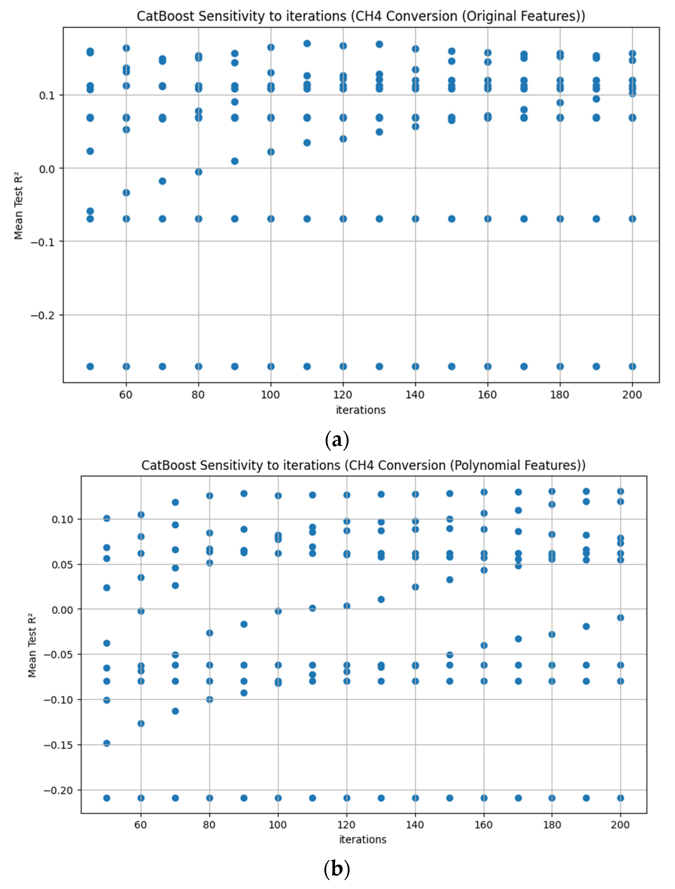
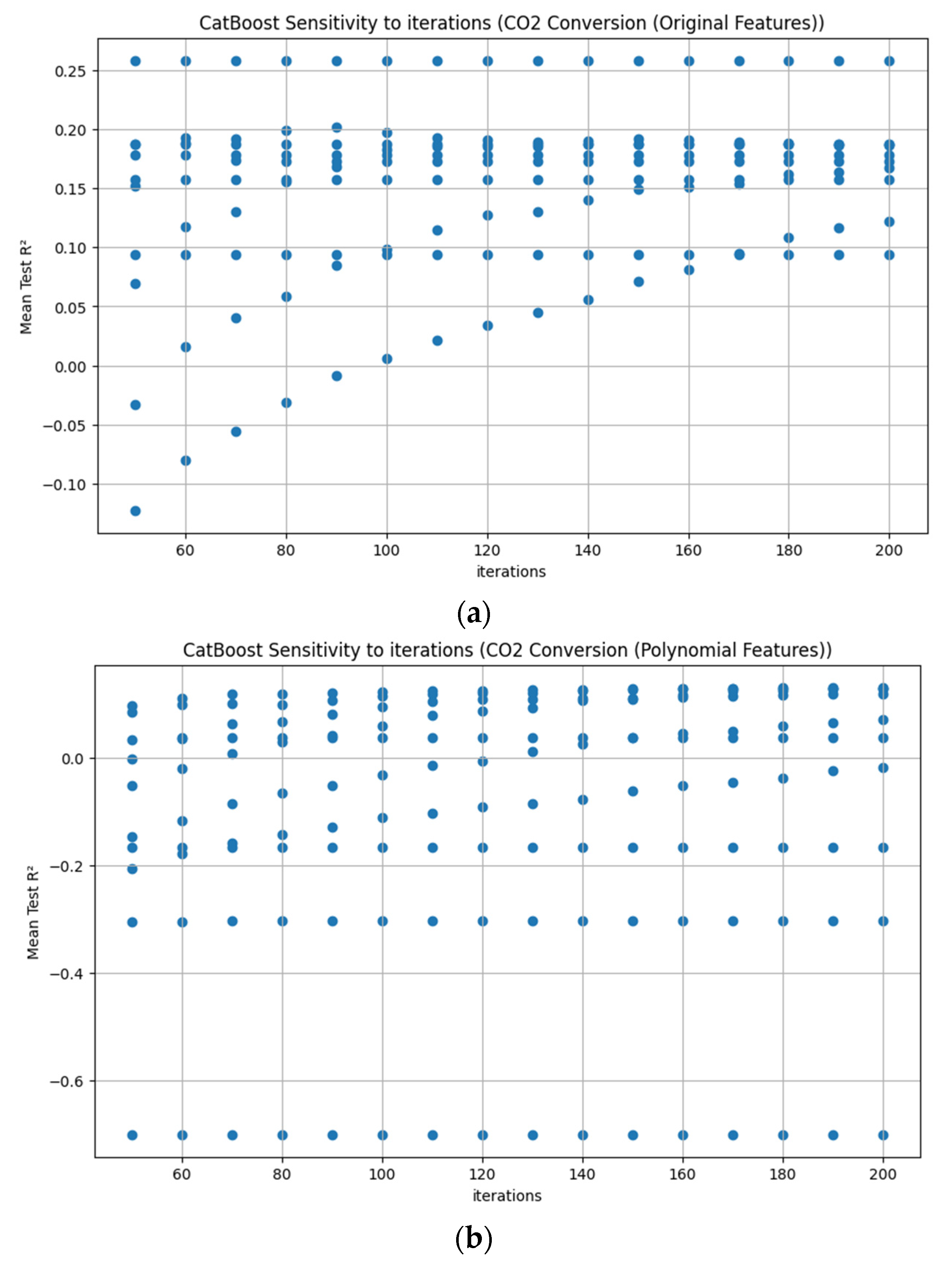
Figure A1. CatBoost Sensitivity to iterations for CH4 Conversion (a) Original Features; (b) Polynomial Features at: 9 different learning rates: 0.01, 0.016, 0.025, 0.04, 0.063, 0.1, 0.158, 0.251, 0.398, 1.0 corresponding to np.logspace (−2, 0, 10).
Energies 18 04807 g0a1
Figure A2. CatBoost Sensitivity to iterations for CO2 Conversion (a) Original Features; (b) Polynomial Features at: 9 different learning rates: 0.01, 0.016, 0.025, 0.04, 0.063, 0.1, 0.158, 0.251, 0.398, 1.0 corresponding to np.logspace (−2, 0, 10).
Energies 18 04807 g0a2
Figure A3. CatBoost Sensitivity to iterations for H2 Conversion (a) Original Features; (b) Polynomial Features at: 9 different learning rates: 0.01, 0.016, 0.025, 0.04, 0.063, 0.1, 0.158, 0.251, 0.398, 1.0 corresponding to np.logspace (−2, 0, 10).
Energies 18 04807 g0a3aEnergies 18 04807 g0a3b
Figure A4. CatBoost Sensitivity to iterations for CO Conversion (a) Original Features; (b) Polynomial Features at: 9 different learning rates: 0.01, 0.016, 0.025, 0.04, 0.063, 0.1, 0.158, 0.251, 0.398, 1.0 corresponding to np.logspace (−2, 0, 10).
Energies 18 04807 g0a4
Figure A5. CatBoost Sensitivity to learning rates for CH4 Conversion (a) Original Features; (b) Polynomial Features.
Energies 18 04807 g0a5
Figure A6. CatBoost Sensitivity to learning rates for CO2 Conversion (a) Original Features; (b) Polynomial Features.
Energies 18 04807 g0a6aEnergies 18 04807 g0a6b
Figure A7. CatBoost Sensitivity to learning rates for H2 Conversion (a) Original Features; (b) Polynomial Features.
Energies 18 04807 g0a7
Figure A8. CatBoost Sensitivity to learning rates for CO Conversion (a) Original Features; (b) Polynomial Features.
Energies 18 04807 g0a8

References

  1. Ayodele, B.V.; Khan, M.R.; Cheng, C.K. Syngas production from CO2 reforming of methane over ceria supported cobalt catalyst: Effects of reactants partial pressure. J. Nat. Gas Sci. Eng. 2015, 27, 1016–1023. [Google Scholar] [CrossRef]
  2. Alenazey, F.S. Utilizing carbon dioxide as a regenerative agent in methane dry reforming to improve hydrogen production and catalyst activity and longevity. Int. J. Hydrogen Energy 2014, 39, 18632–18641. [Google Scholar] [CrossRef]
  3. Augusto, B.; Marco, P.; Cesare, S. Solar steam reforming of natural gas integrated with a gas turbine power plant. Sol. Energy 2013, 96, 46–55. [Google Scholar] [CrossRef]
  4. Dean, J.A. Lange’s Handbook of Chemistry, 12th ed.; McGraw-Hill: New York, NY, USA, 1979. [Google Scholar]
  5. Alper, E.; Orhan, O.Y. CO2 utilization: Developments in conversion processes. Petroleum 2017, 3, 109–126. [Google Scholar] [CrossRef]
  6. Braga, T.P.; Santos, R.C.; Sales, B.M.; da Silva, B.R.; Pinheiro, A.N.; Leite, E.R.; Valentini, A. CO2 mitigation by carbon nanotube formation during dry reforming of methane analyzed by factorial design combined with response surface methodology. Chin. J. Catal. 2014, 35, 514–523. [Google Scholar] [CrossRef]
  7. Hossain, M.A.; Ayodele, B.V.; Cheng, C.K.; Khan, M.R. Artificial neural network modeling of hydrogen-rich syngas production from methane dry reforming over novel Ni/CaFe2O4 catalysts. Int. J. Hydrogen Energy 2016, 41, 11119–11130. [Google Scholar] [CrossRef]
  8. Lavoie, J.-M. Review on dry reforming of methane, a potentially more environmentally-friendly approach to the increasing natural gas exploitation. Front. Chem. 2014, 2, 81. [Google Scholar] [CrossRef]
  9. Nikoo, M.K.; Amin, N. Thermodynamic analysis of carbon dioxide reforming of methane in view of solid carbon formation. Fuel Process. Technol. 2011, 92, 678–691. [Google Scholar] [CrossRef]
  10. Sodesawa, T.; Dobashi, A.; Nozaki, F. Catalytic reaction of methane with carbon dioxide. React. Kinet. Catal. Lett. 1979, 12, 107–111. [Google Scholar] [CrossRef]
  11. Mohamad, H.A. A Mini-Review on CO2 Reforming of Methane. Prog. Petrochem. Sci. 2018, 2, 532. [Google Scholar] [CrossRef]
  12. Rostrup-Nielsen, J.R. Catal. Today 1993, 18, 305–324. [Google Scholar] [CrossRef]
  13. Fan, M.; Abdullah, A.Z.; Bhatia, S. Catalytic technology for carbon dioxide reforming of methane to synthesis gas. ChemCatChem 2009, 1, 192–208. [Google Scholar] [CrossRef]
  14. García-Vargas, J.M.; Valverde, J.L.; Dorado, F.; Sánchez, P. Influence of the support on the catalytic behaviour of Ni catalysts for the dry reforming reaction and the tri-reforming process. J. Mol. Catal. A Chem. 2014, 395, 108–116. [Google Scholar] [CrossRef]
  15. Devasahayam, S. Catalytic actions of MgCO3/MgO system for efficient carbon reforming processes. Sustain. Mater. Technol. 2019, 22, e00122. [Google Scholar] [CrossRef]
  16. Devasahayam, S. Review: Opportunities for simultaneous energy/materials conversion of carbon dioxide and plastics in metallurgical processes. Sustain. Mater. Technol. 2019, 22, 119883. [Google Scholar] [CrossRef]
  17. Devasahayam, S.; Strezov, V. Thermal decomposition of magnesium carbonate with biomass and plastic wastes for simultaneous production of hydrogen and carbon avoidance. J. Clean. Prod. 2018, 174, 1089–1095. [Google Scholar] [CrossRef]
  18. Devasahayam, S. Decarbonising the Portland and Other Cements—Via Simultaneous Feedstock Recycling and Carbon Conversions Sans External Catalysts. Polymers 2021, 13, 2462. [Google Scholar] [CrossRef]
  19. IRENA. Breakthrough Agenda Report 2023—Hydrogen; International Energy Agency: Paris, France, 2023. [Google Scholar]
  20. Hydrogen Council and McKinsey and Company. Hydrogen Insights 2024; Hydrogen Council: Rotterdam, The Netherlands, 2024. [Google Scholar]
  21. Cozzolino, R.; Bella, G. A review of electrolyzer-based systems providing grid ancillary services: Current status, market, challenges and future directions. Front. Energy Res. 2024, 12, 1358333. [Google Scholar] [CrossRef]
  22. Fu, H.; Wang, Z.; Nichani, E.; Lee, J.D. Learning Hierarchical Polynomials of Multiple Nonlinear Features with Three-Layer Networks. arXiv 2024, arXiv:2411.17201. [Google Scholar] [CrossRef]
  23. Devasahayam, S. Deep learning models in Python for predicting hydrogen production: A comparative study. Energy 2023, 280, 128088. [Google Scholar] [CrossRef]
  24. Devasahayam, S.; Albijanic, B. Predicting hydrogen production from co-gasification of biomass and plastics using tree based machine learning algorithms. Renew. Energy 2023, 222, 119883. [Google Scholar] [CrossRef]
  25. Breiman, L.; Cutler, A. Random Forests. J. Mach. Learn. Res. 2001, 45, 5–32. [Google Scholar] [CrossRef]
  26. Rocca, J. Ensemble Methods: Bagging, Boosting and Stacking 2019. Available online: https://towardsdatascience.com/ensemble-methods-bagging-boosting-and-stacking-c9214a10a205 (accessed on 5 May 2022).
  27. Lasso and Ridge Regression in Python Tutorial. Available online: https://www.datacamp.com/tutorial/tutorial-lasso-ridge-regression (accessed on 5 May 2022).
  28. Chinda, A.; Derevlev, N. Support Vector Machines: An Overview of Optimization Techniques and Model Selection; CRC Press: Boca Raton, FL, USA, 2023. [Google Scholar]
  29. Choudhury, A. AdaBoost vs. Gradient Boosting: A Comparison of Leading Boosting Algorithms, 18 January 2021. Available online: https://analyticsindiamag.com/adaboost-vs-gradient-boosting-a-comparison-of-leading-boosting-algorithms/#:~:text=AdaBoost%20is%20the%20first%20designed,Boosting%20more%20flexible%20than%20AdaBoost (accessed on 13 December 2022).
  30. Scikit-learn. Gradient Boosting Regression, 2010–2016. Available online: https://scikit-learn.org/0.18/auto_examples/ensemble/plot_gradient_boosting_regression.html#sphx-glr-auto-examples-ensemble-plot-gradient-boosting-regression-py (accessed on 16 December 2022).
  31. Scikit-learn. Gradient Boosting Regression, 2007–2022. Available online: https://scikit-learn.org/stable/auto_examples/ensemble/plot_gradient_boosting_regression.html#sphx-glr-auto-examples-ensemble-plot-gradient-boosting-regression-py (accessed on 16 December 2022).
  32. Devasahayam, S. Advancing Flotation Process Modeling: Bayesian vs. Sklearn Approaches for Gold Grade Prediction. Minerals 2025, 15, 591. [Google Scholar] [CrossRef]
  33. Pedregosa, F.; Varoquaux, G.; Gramfort, A.; Michel, V.; Thirion, B.; Grisel, O.; Blondel, M.; Prettenhofer, P.; Weiss, R.; Dubourg, V.; et al. Scikit-learn: Machine Learning in Python: Cross-validation: Evaluating estimator performance. J. Mach. Learn. Res 2011, 12, 2825–2830. [Google Scholar]
  34. Brownlee, J. Ensemble Learning: Gradient Boosting with Scikit-Learn, XGBoost, LightGBM, and CatBoost, 27 April 2021. Available online: https://machinelearningmastery.com/gradient-boosting-with-scikit-learn-xgboost-lightgbm-and-catboost/ (accessed on 7 December 2022).
  35. Clyde, M.; Çetinkaya-Rundel, M.; Rundel, C.; Banks, D.; Chai, C.; Huang, L. An Introduction to Bayesian Thinking A Companion to the Statistics with R Course; 2022. Available online: https://bookdown.org (accessed on 23 August 2025).
  36. Brownlee, J. How to Develop Elastic Net Regression Models in Python, 12 June 2020. Available online: https://machinelearningmastery.com/elastic-net-regression-in-python/ (accessed on 23 August 2025).
  37. Hastie, T.; Tibshirani, R.; Friedman, J. Elements of Statistical Learning, 2nd ed.; Springer: Berlin/Heidelberg, Germany, 2009. [Google Scholar]
  38. Yorkinov. Regression Accuracy Check in Python (MAE, MSE, RMSE, R-Squared), 10 October 2019. Available online: https://www.datatechnotes.com/2019/10/accuracy-check-in-python-mae-mse-rmse-r.html (accessed on 23 August 2025).
  39. Alawi, N.; Barifcani, A.; Abid, H. Optimisation of CH4 and CO2 conversion and selectivity of H2 and CO for the dry re-forming of methane by a microwave plasma technique using a Box-Behnken design. Asia Pac. J. Chem. Eng. 2018, 13, e2254. [Google Scholar] [CrossRef]
  40. Jiayin, L.; Jing, X.; Evgeny, R.; Annemie, B. Machine learning-based prediction and optimization of plasma-catalytic dry reforming of methane in a dielectric barrier discharge reactor. Chem. Eng. J. 2025, 507, 159897. [Google Scholar]
  41. Jiayin, L.; Jing, X.; Evgeny, R.; Bart, W.; Annemie, B. Machine learning-based prediction and optimization of plasma-based conversion of CO2 and CH4 in an atmospheric pressure glow discharge plasma. Green Chem. 2025, 27, 3916–3931. [Google Scholar]
  42. Alotaibi, F.N.; Berrouk, A.S.; Salim, I.M. Scaling up dry methane reforming: Integrating computational fluid dynamics and machine learning for enhanced hydrogen production in industrial-scale fluidized bed reactors. Fuel 2024, 376, 132673. [Google Scholar] [CrossRef]
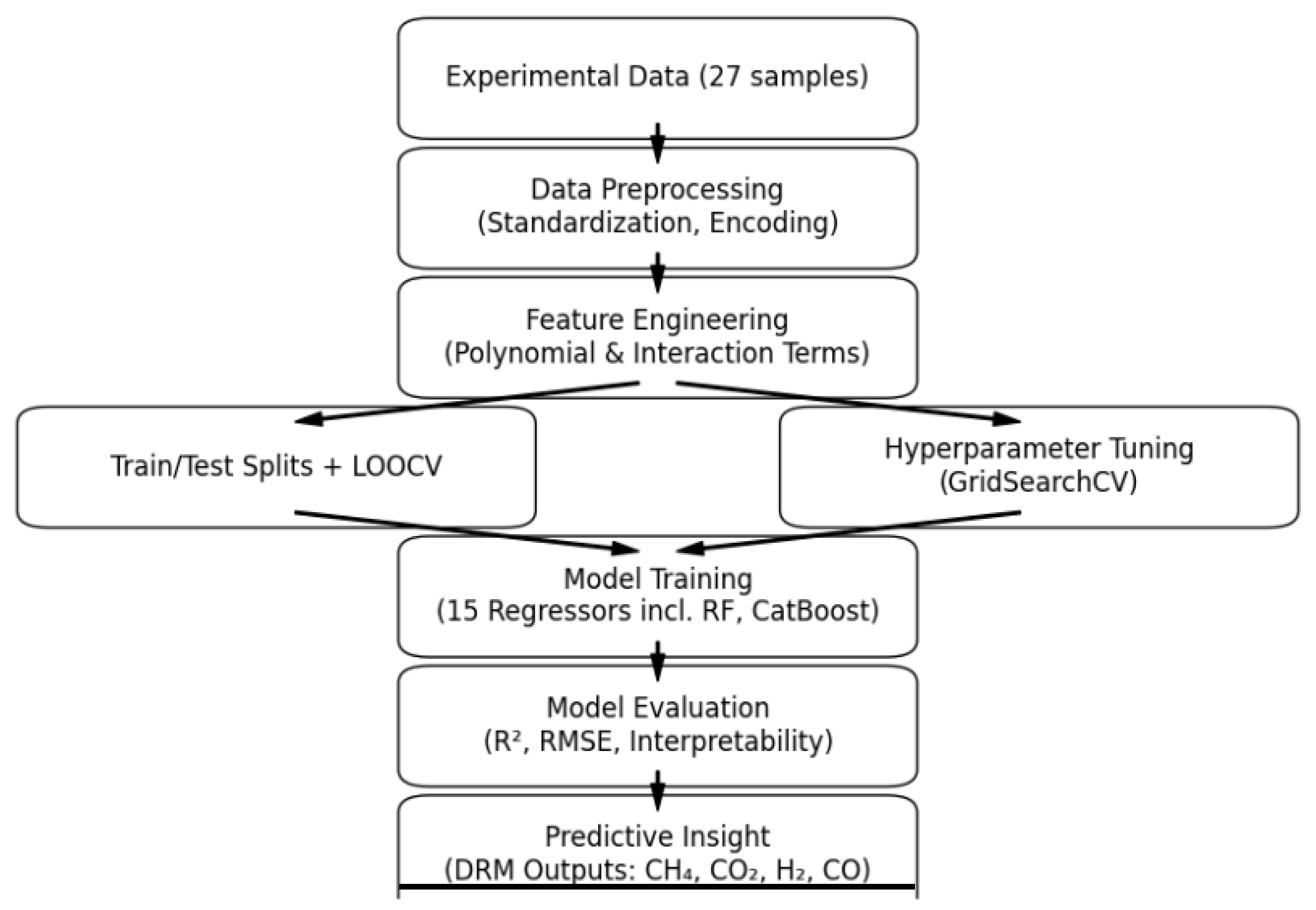
Figure 1. A flowchart summarizing model training and evaluation.
Energies 18 04807 g001
Figure 2. Visualizing the data.
Energies 18 04807 g002
Figure 3. Correlation matrix using the features and the target variables.
Energies 18 04807 g003
Figure 4. Predicted vs. actual data using Grid Search CV for CH4 Conversion for test data (a) original features, (b) polynomial features.
Energies 18 04807 g004aEnergies 18 04807 g004b
Figure 5. Predicted vs. actual data using GridSearch CV for CO2 Conversion for Test data (a) original features, (b) polynomial features.
Energies 18 04807 g005
Figure 6. Predicted vs. actual data using GridSearch CV for H2 Conversion for Test data (a) original features, (b) polynomial features.
Energies 18 04807 g006aEnergies 18 04807 g006b
Figure 7. Predicted vs. actual data using GridSearch CV for CO Conversion for Test data (a) original features, (b) polynomial features.
Energies 18 04807 g007aEnergies 18 04807 g007b
Figure 8. Parity plots for ANN-MLP and ANN-RBF models trained on DRM dataset and evaluated on test data (70:30 split). R2 values are shown for each model and target.
Energies 18 04807 g008
Figure 9. Predicted vs. actual values using LOOCV for Random Forest Predictions. (a) original data; (b) after removing the outliers.
Energies 18 04807 g009
Figure 10. Predicted vs. actual values using LOOCV for Gradient Boosting Predictions. (a) original data; (b) after removing the outliers.
Energies 18 04807 g010
Figure 11. Regression model Metrics for CH4 Conversion; (a) Mean Absolute Error; (b) Root Mean Squared Error.
Energies 18 04807 g011
Figure 12. Regression model Metrics for CO2 Conversion; (a) Mean Absolute Error; (b) Root Mean Squared Error.
Energies 18 04807 g012
Figure 13. Regression model Metrics for H2 Yield; (a) Mean Absolute Error; (b) Root Mean Squared Error.
Energies 18 04807 g013
Figure 14. Regression model Metrics for CO Yield; (a) Mean Absolute Error; (b) Root Mean Squared Error.
Energies 18 04807 g014
Table 1. Comparison of Hydrogen Production Methods.
Hydrogen Production MethodReactionFeedstocksTypical H2/CO RatioCO2 Emissions (kg CO2/kg H2)Energy EfficiencyFuel Relevance
Steam Methane Reforming (SMR) [19,20]CH4 + H2O → CO + 3H2CH4, H2O (steam)~3.0~9–11~65–75%Dominant method; high emissions
Dry Reforming of Methane (DRM) [8,9]CH4 + CO2 → 2CO + 2H2CH4, CO2~1.0~5–7~55–65%Syngas for Fischer–Tropsch, methanol, SNG
Electrolysis (Renewable) [21]H2O → H2 + ½O2
(via electricity)
Water + Renewable Power∞ (pure H2)0 (if fully renewable)~60–70%Green hydrogen; no carbon-based fuel generated
Table 2. Descriptive statistics of the data.
Feed RatioReaction TempMetal LoadingCH4 ConversionCO2 ConversionH2 YieldCO Yield
count27.0027.0027.0027.0027.0027.0027.00
mean0.70750.0010.0038.3235.8423.0723.98
std0.2541.604.1619.9320.2415.7715.84
min0.40700.005.0017.6914.1511.1213.09
25%0.40700.005.0024.3921.2413.4614.81
50%0.70750.0010.0032.8930.0217.1518.32
75%1.00800.0015.0045.1543.2926.3326.43
max1.00800.0015.0090.0487.6073.4274.43
Table 3. Identifying potential outliers.
VariableQ1Q3IQRLower BoundUpper BoundPotential Outliers
Feed_ratio0.401.000.60−0.501.90None
Reaction_Temp700.00800.00100.00550.00950.00None
Metal_loading5.0015.0010.00−10.0030.00None
CH4_conversion24.3945.1520.76−6.7576.29<−6.75; >76.29
CO2_conversion21.2443.2922.05−11.8376.36<−11.83; >76.36
H2_yield13.4626.3312.87−6.8546.64<−6.85; >46.64
CO_yield14.8126.4311.62−2.6243.86<−2.62; >43.86
Table 4. Pearson Correlation Coefficients (PCC) between input features and DRM outputs.
FeatureCH4 ConversionCO2 ConversionH2 YieldCO Yield
Feed Ratio0.590.640.430.44
Reaction Temperature0.430.500.460.42
Metal Loading0.310.290.330.37
Feed Ratio × Temperature0.660.700.580.61
Table 5. Regression model Metrics (R2 and MSE values) for original and polynomial features CV = 5.
CH4 Conversion
FeaturesModelTrain R2Test R2Train MSETest MSE
OriginalLinear Regression0.550.24184.20102.13
OriginalRidge Regression0.550.34184.6188.90
OriginalLasso Regression0.540.48187.4170.35
OriginalElasticNet0.550.44186.0076.15
OriginalBayesian Ridge0.540.49187.3169.21
OriginalRandom Forest0.930.8427.1721.54
OriginalGradient Boosting0.740.76108.0731.99
OriginalExtra Trees1.00−1.000.00270.33
OriginalSVR0.520.87199.6617.89
OriginalNuSVR0.510.87199.6818.22
OriginalKernel Ridge0.830.2969.0896.55
OriginalXGBoost1.000.420.0079.08
OriginalLightGBM0.00−0.12411.68151.17
OriginalCatBoost0.910.9135.5712.19
OriginalMLP Regressor0.81−0.0376.24139.37
PolyLinear Regression0.82−0.0172.95136.13
PolyRidge Regression0.590.43168.4077.64
PolyLasso Regression0.770.6694.0246.37
PolyElasticNet0.770.6194.6052.83
PolyBayesian Ridge0.570.31178.0692.65
PolyRandom Forest0.920.9333.169.29
PolyGradient Boosting0.950.9419.827.58
PolyExtra Trees1.00−0.270.00171.21
PolySVR−0.030.24423.73102.40
PolyNuSVR−0.070.18441.99111.03
PolyKernel Ridge0.96−8.9415.821344.17
PolyXGBoost0.930.6428.0048.13
PolyLightGBM0.00−0.12411.68151.17
PolyCatBoost1.000.930.009.80
PolyMLP Regressor−0.23−0.24505.51167.62
CO2 Conversion
OriginalLinear Regression0.600.09167.62124.03
OriginalRidge Regression0.600.11167.63122.36
OriginalLasso Regression0.600.34170.8389.60
OriginalElasticNet0.600.31169.6493.78
OriginalBayesian Ridge0.600.33169.9092.09
OriginalRandom Forest0.910.8038.1027.30
OriginalGradient Boosting0.910.7338.8436.99
OriginalExtra Trees1.00−0.790.00244.22
OriginalSVR0.490.93217.7210.18
OriginalNuSVR0.480.92218.4010.64
OriginalKernel Ridge0.840.1069.31122.58
OriginalXGBoost1.000.160.00114.28
OriginalLightGBM0.00−0.18423.91161.43
OriginalCatBoost0.920.8732.8917.74
OriginalMLP Regressor0.81−0.2380.68167.99
PolyLinear Regression0.84−0.2667.26172.18
PolyRidge Regression0.640.28152.9298.17
PolyLasso Regression0.780.5892.4058.05
PolyElasticNet0.790.5589.9461.13
PolyBayesian Ridge0.620.14161.32117.54
PolyRandom Forest0.930.9631.625.74
PolyGradient Boosting1.000.991.001.99
PolyExtra Trees1.00−0.420.00194.76
PolySVR−0.090.01463.14135.56
PolyNuSVR−0.120.12472.79120.34
PolyKernel Ridge0.97−7.2214.451124.21
PolyXGBoost0.930.7627.7332.49
PolyLightGBM0.00−0.18423.91161.43
PolyCatBoost1.001.000.010.57
PolyMLP Regressor−0.10−0.01464.30138.71
H2 Yield
OriginalLinear Regression0.49−2.28133.81105.28
OriginalRidge Regression0.49−2.24133.81104.06
OriginalLasso Regression0.49−2.16133.84101.33
OriginalElasticNet0.49−1.81134.2590.20
OriginalBayesian Ridge0.48−1.16136.7369.42
OriginalRandom Forest0.910.8823.733.72
OriginalGradient Boosting0.61−0.05103.6333.78
OriginalExtra Trees1.000.810.006.24
OriginalSVR0.500.55130.9714.49
OriginalNuSVR0.510.68129.5810.16
OriginalKernel Ridge0.81−2.8149.93122.31
OriginalXGBoost0.500.02132.1731.30
OriginalLightGBM0.00−0.79262.7457.36
OriginalCatBoost0.930.8518.124.67
OriginalMLP Regressor0.76−4.8262.78186.81
PolyLinear Regression0.78−4.1456.55164.95
PolyRidge Regression0.54−1.76121.5088.58
PolyLasso Regression0.76−2.1463.15100.70
PolyElasticNet0.70−0.7978.1457.43
PolyBayesian Ridge0.51−2.11128.0399.75
PolyRandom Forest0.910.6622.3710.80
PolyGradient Boosting0.610.23103.3324.87
PolyExtra Trees1.000.310.0022.13
PolySVR−0.010.48266.6716.58
PolyNuSVR−0.030.48271.3716.73
PolyKernel Ridge0.97−10.796.79378.17
PolyXGBoost0.500.19131.3825.90
PolyLightGBM0.00−0.79262.7457.36
PolyCatBoost1.000.840.005.17
PolyMLP Regressor−0.00−0.55263.4249.74
CO Yield
OriginalLinear Regression0.48−1.68138.3197.79
OriginalRidge Regression0.48−1.65138.3196.69
OriginalLasso Regression0.48−1.59138.3494.21
OriginalElasticNet0.47−1.31138.7484.13
OriginalBayesian Ridge0.46−0.75141.5363.83
OriginalRandom Forest0.89−0.0029.6836.56
OriginalGradient Boosting0.620.21101.3228.90
OriginalExtra Trees1.00−0.340.0048.71
OriginalSVR0.430.82151.506.67
OriginalNuSVR0.460.76141.578.64
OriginalKernel Ridge0.80−2.4951.58127.00
OriginalXGBoost0.490.17133.4530.14
OriginalLightGBM−0.00−0.93263.6370.22
OriginalCatBoost0.930.7917.657.64
OriginalMLP Regressor0.74−3.8668.31177.14
PolyLinear Regression0.77−3.6759.74170.11
PolyRidge Regression0.52−1.35127.3285.69
PolyLasso Regression0.68−0.4383.0952.07
PolyElasticNet0.69−0.4681.6853.16
PolyBayesian Ridge0.50−1.54132.3492.41
PolyRandom Forest0.890.1327.9631.82
PolyGradient Boosting0.610.11102.2132.43
PolyExtra Trees1.00−0.920.0070.13
PolySVR−0.050.33277.5324.40
PolyNuSVR−0.070.33281.1324.33
PolyKernel Ridge0.97−9.727.19390.50
PolyXGBoost0.750.5066.9118.17
PolyLightGBM−0.00−0.93263.6370.22
PolyCatBoost1.000.890.013.97
PolyMLP Regressor−0.00−0.63264.7059.26
Table 6. LOOCV performance metrics before and after removal of the outliers.
ModelTargetFeature TypeR2 After Removal of OutliersMSE After Removal of OutliersR2 Without Removal of OutliersMSE Without Removal of Outliers
Random ForestCH4_conversionOriginal0.6860.790.39232.70
Gradient BoostingCH4_conversionOriginal0.6271.440.47203.60
SVRCH4_conversionOriginal−0.07201.26−0.00383.03
CatBoostCH4_conversionOriginal0.5585.050.22296.99
Random ForestCH4_conversionPolynomial0.5977.480.33256.60
Gradient BoostingCH4_conversionPolynomial0.5976.470.17317.54
SVRCH4_conversionPolynomial−0.17221.06−0.09415.53
CatBoostCH4_conversionPolynomial0.42108.880.18314.33
Random ForestCO2_conversionOriginal0.8629.200.45216.55
Gradient BoostingCO2_conversionOriginal0.8236.190.44222.20
SVRCO2_conversionOriginal0.01201.30−0.04408.69
CatBoostCO2_conversionOriginal0.6865.260.26292.33
Random ForestCO2_conversionPolynomial0.7746.090.40235.11
Gradient BoostingCO2_conversionPolynomial0.8236.060.16329.38
SVRCO2_conversionPolynomial−0.06216.97−0.10432.73
CatBoostCO2_conversionPolynomial0.6081.570.25295.61
Random ForestH2_yieldOriginal0.4131.200.30168.51
Gradient BoostingH2_yieldOriginal0.3136.290.29169.16
SVRH2_yieldOriginal0.0649.88−0.04250.12
CatBoostH2_yieldOriginal0.3235.800.21188.09
Random ForestH2_yieldPolynomial0.2042.470.08220.01
Gradient BoostingH2_yieldPolynomial0.1544.970.19192.93
SVRH2_yieldPolynomial−0.0957.82−0.12267.80
CatBoostH2_yieldPolynomial0.2539.930.23183.36
Random ForestCO_yieldOriginal0.6914.250.27176.98
Gradient BoostingCO_yieldOriginal0.7212.820.27175.99
SVRCO_yieldOriginal0.1041.98−0.02246.21
CatBoostCO_yieldOriginal0.5023.030.18197.30
Random ForestCO_yieldPolynomial0.4525.410.06226.24
Gradient BoostingCO_yieldPolynomial0.5620.200.09220.04
SVRCO_yieldPolynomial−0.0649.14−0.08261.20
CatBoostCO_yieldPolynomial0.4127.440.17200.38
Disclaimer/Publisher’s Note: The statements, opinions and data contained in all publications are solely those of the individual author(s) and contributor(s) and not of MDPI and/or the editor(s). MDPI and/or the editor(s) disclaim responsibility for any injury to people or property resulting from any ideas, methods, instructions or products referred to in the content.