Comparative Performance Analysis of Deep Learning-Based Diagnostic and Predictive Models in Grid-Integrated Doubly Fed Induction Generator Wind Turbines

Abstract

As the deployment of wind energy systems continues to rise globally, ensuring the reliability and efficiency of grid-connected Doubly Fed Induction Generator (DFIG) wind turbines has become increasingly critical. Two core challenges faced by these systems include fault diagnosis in power electronic converters and accurate prediction of wind conditions for adaptive power control. Recent advancements in artificial intelligence (AI) have introduced powerful tools for addressing these challenges. This study presents the first unified comparative performance analysis of two deep learning-based models: (i) a Convolutional Neural Network-Long Short-Term Memory CNN-LSTM with Variational Mode Decomposition for real-time Grid Side Converter (GSC) fault diagnosis, and (ii) an Incremental Generative Adversarial Network (IGAN) for wind attribute prediction and adaptive droop gain control, applied to grid-integrated DFIG wind turbines. Unlike prior studies that address fault diagnosis and wind forecasting separately, both models are evaluated within a common MATLAB/Simulink framework using identical wind profiles, disturbances, and system parameters, ensuring fair and reproducible benchmarking. Beyond accuracy, the analysis incorporates multi-dimensional performance metrics such as inference latency, robustness to disturbances, scalability, and computational efficiency, offering a more holistic assessment than prior work. The results reveal complementary strengths: the CNN-LSTM achieves 88% accuracy with 15 ms detection latency for converter faults, while the IGAN delivers more than 95% prediction accuracy and enhances frequency stability by 18%. Comparative analysis shows that while the CNN-LSTM model is highly suitable for rapid fault localization and maintenance planning, the IGAN model excels in predictive control and grid performance optimization. Unlike prior studies, this work establishes the first direct comparative framework for diagnostic and predictive AI models in DFIG systems, providing novel insights into their complementary strengths and practical deployment trade-offs. This dual evaluation lays the groundwork for hybrid two-tier AI frameworks in smart wind energy systems. By establishing a reproducible methodology and highlighting practical deployment trade-offs, this study offers valuable guidance for researchers and practitioners seeking explainable, adaptive, and computationally efficient AI solutions for next-generation renewable energy integration.

1. Introduction

The global transition toward clean and renewable energy has placed wind energy at the forefront of sustainable power generation. Wind turbines play a pivotal role in the worldwide transition to renewable energy by harnessing wind power to generate electricity [1]. As a stable and environmentally friendly alternative to fossil fuels, they contribute significantly to reducing carbon emissions and combating climate change. Among the available renewable energy sources, solar, tidal, and wind energy have emerged as leading options for many countries due to their minimal environmental footprint, clean energy output, and widespread availability. Compared to solar and tidal energy, wind energy is generally easier and more cost-effective to develop on a large scale [2]. As a result, it remains one of the fastest-growing renewable energy sources globally. However, the inherent variability and intermittency of wind pose operational and management challenges in power systems [3]. Among the available wind turbine technologies, the DFIG-based wind turbine system is extensively adopted due to its capability for variable speed operation, high energy conversion efficiency, and reduced converter cost by controlling only a fraction of the total power [4,5].

Despite these advantages, DFIG-based systems face two critical operational challenges. First, electrical faults in power electronic components [6], especially the IGBTs of the GSC, can compromise system stability, increase downtime, and lead to financial losses if not detected promptly. Second, the highly stochastic nature of wind patterns introduces difficulties in predicting wind behavior, thereby affecting power quality, voltage regulation, and synchronization with the grid [4].

To address the first challenge, ref. [5] proposed a CNN-LSTM hybrid model combined with VMD for real-time fault diagnosis of GSC side IGBT modules. This model automatically extracts time–frequency domain features from current signals under ten distinct fault scenarios and achieves an impressive classification accuracy of 88.1%, even under noisy conditions. The model is designed in MATLAB/Simulink and demonstrates the ability to detect faults with low latency and high reliability, making it highly suitable for real-time deployment in smart grid environments [5].

In parallel, to tackle the challenge of wind unpredictability [4], the authors developed an Incremental Tuned Generative Adversarial Network (IGAN) model that incorporates self-attention mechanisms, a dual discriminator architecture, and adaptive training to forecast wind speed, droop gain, and power injection patterns. This model outperforms classical neural networks by achieving prediction accuracies above 95% and reducing the mean absolute error (MAE) to less than 2% in key power regulation parameters. It is further validated using a dynamic simulation model of a DFIG-based wind turbine, showing effective improvement in grid synchronization and frequency regulation [4].

Although both models demonstrate strong individual performance in their respective domains, fault detection and predictive control, a comparative evaluation is lacking in the current literature. Understanding the trade-offs between diagnostic precision and predictive adaptability, latency, scalability, and computational efficiency is essential for guiding the integration of AI in modern wind energy systems [7]. Moreover, such comparative insights can inform the design of hybrid AI frameworks [8] that combine diagnostic and predictive functionalities to create robust and autonomous DFIG control systems [9].

This article differs materially from our earlier studies in [4,5]. Paper [5] introduced a VMD-CNN-LSTM diagnostic classifier for GSC IGBT faults in a DFIG and reported accuracy/latency under noisy conditions (88% accuracy; fast detection) within a standalone diagnostic context. By contrast, paper [4] presented an incremental, self-attention GAN for short-horizon wind/power forecasting and droop-gain tuning, achieving >95% predictive accuracy in a predictive control context. The present work does not propose yet another new model; instead, it unifies these two prior lines by placing both models in the same MATLAB/Simulink DFIG environment with identical wind profiles, parameters, and disturbance scripts, and evaluates them with harmonized metrics (including latency and system-level frequency support). We further analyze their complementarity as a two-tier strategy and show a combined ≈18% reduction in peak frequency deviation versus a non-predictive baseline evidence absent from [4,5].

Predictive control in DFIG wind farms hinges on turbine and grid-level variables observed via SCADA. In this study, hub-height wind speed V, active power output P, and grid frequency deviation Δf are treated as the primary predictors for short-horizon forecasting and droop-gain adaptation; these signals are continuously recorded in modern turbines and capture both the exogenous wind forcing and its system-level impact. Consistent with this focus, the IGAN consumes standardized, windowed sequences of V, P, and Δf (50 input steps → 10 forecast steps). This clarifies that our predictive task targets the operational quantities most salient to frequency support and power regulation.

1.1. Identified Research Gaps

Despite significant advancements in the application of deep learning models for the monitoring and control of grid-integrated DFIG-based wind turbines, several critical gaps remain in the existing body of research:

• Lack of comparative studies between diagnostic and predictive AI models.

Existing research often explores either fault diagnosis or wind parameter prediction in isolation. For example, ref. [5] focused solely on real-time GSC fault detection using a CNN-LSTM model, whereas ref. [4] developed an Incremental GAN for wind prediction and droop gain optimization. However, there is no unified comparative framework evaluating the diagnostic performance versus predictive accuracy of these models under consistent operational and computational environments.

• Limited evaluation of cross-domain model interoperability.

Modern wind turbine systems require both high-fidelity diagnostics for reliability and accurate forecasting for operational efficiency. Yet, the literature [4,5] lacks an analysis of whether these AI models can be synergistically integrated or deployed in tandem. The interplay between fault prediction (e.g., GSC IGBT degradation) and environmental condition forecasting (e.g., wind speed variability) remains unexplored.

• Insufficient focus on real-time applicability and resource constraints.

While many studies report high accuracy for standalone models (88.1% for CNN-LSTM and >95% for Incremental GAN), researchers rarely compare their real-time inference time, computational complexity, and latency under varying data conditions. This leaves a gap in understanding their suitability for embedded deployment in smart wind turbine controllers.

• Scarcity of analysis on explainability and model robustness.

Deep learning models often operate as black boxes. Neither [4] nor [5] explicitly evaluates the interpretability of their models’ decisions, which is crucial for human operators and grid regulators. Furthermore, there is limited discussion on robustness to adversarial conditions, such as noisy signals or abrupt weather changes.

This paper aims to fill this research gap by presenting a comparative performance analysis of the CNN-LSTM-based fault diagnostic model [5] and the Incremental GAN-based wind prediction model [4]. Both models are implemented and evaluated within a unified simulation environment using consistent metrics such as classification/prediction accuracy, execution time, model robustness, and interpretability. By doing so, we seek to provide a comprehensive understanding of their relative strengths, limitations, and practical suitability in real-time grid-integrated wind turbine applications.

1.2. Key Contributions of This Study

• To address the above gaps, this study makes the following contributions:

• Unified comparative analysis of two deep learning models.

The authors conduct the first detailed comparative evaluation of a CNN-LSTM-based fault diagnostic model [5] and an Incremental GAN-based wind attribute prediction model [4], both are applied to DFIG wind turbine systems. The models are assessed under a consistent simulation framework using MATLAB/Simulink to ensure fair benchmarking.

• Multi-metric evaluation across diagnostic and predictive tasks.

The authors assess the models using a comprehensive set of performance metrics, including classification/prediction accuracy, MAE, execution time, model scalability, and robustness to signal noise and data shifts. This multi-angle comparison provides insights into each model’s strengths and limitations in practical scenarios.

• Analysis of real-time suitability and computational trade-offs.

This study evaluates the inference speed and resource efficiency of both models on real-time data streams. We also investigate hybrid deployment by using the CNN-LSTM for hardware-level fault detection and the IGAN for generating adaptive control signals.

• Recommendations for model selection based on operational priorities.

Based on the comparative results, the authors propose a decision framework for selecting diagnostic vs. predictive models based on system-level priorities (e.g., maintenance scheduling, frequency regulation, or fault recovery planning). This guidance supports the design of intelligent wind turbine control systems with modular AI integration.

• Foundation for future hybrid explainable AI systems in wind energy.

By revealing the complementary nature of fault diagnosis and wind prediction models, this study lays the groundwork for developing multi-agent or hybrid AI architectures combining both functionalities, augmented with explainability tools for enhanced transparency and trustworthiness.

1.3. Background and Related Work

1.3.1. Background

DFIG-based turbines dominate utility-scale wind owing to variable-speed operation, partial-converter efficiency, and grid-support capability [3,10,11,12]. Their partial back-to-back converter interface (RSC/GSC) increases sensitivity to grid disturbances, making LVRT compliance essential [13,14,15,16]. In practice, GSC IGBTs are fault-prone and wind variability challenges frequency and power-quality performance; modern SCADA platforms capture wind speed, currents, power, and frequency for monitoring, diagnosis, and control [17,18,19].

Reliable grid integration requires (i) fast detection/isolation of converter faults, especially GSC IGBTs, before DC-link excursions and current limits are violated, and (ii) short-horizon forecasting of wind-driven variations to stabilize frequency and power quality [4,5]. Prior studies seldom provide a like-for-like comparison of diagnostic vs. predictive AI on the same DFIG plant under identical wind profiles, parameters, disturbance scripts, metrics, and compute budgets; latency and system-level impacts are also inconsistently reported [20,21,22,23,24,25,26]. This lack of standardized evaluation obscures trade-offs and limits guidance for coordinated control design.

1.3.2. Status

Two AI streams address these needs separately: a VMD-enhanced CNN-LSTM for rapid GSC-IGBT fault diagnosis (high accuracy/low latency) [5], and an incremental, self-attention IGAN for short-term wind/power forecasting and droop-gain tuning [4].

1.3.3. Novelty

The authors provide the first unified comparative analysis of a diagnostic model (CNN-LSTM) and a predictive model (IGAN) on one DFIG platform with identical wind/input conditions and evaluation settings; we assess multi-metric, real-time feasibility (including latency) and system-level impact (frequency-deviation reduction), and we demonstrate complementarity as a dual-layer strategy for hybrid deployment. In our experiments, the integrated approach reduces peak frequency deviation by ~18% vs. a non-predictive baseline.

1.4. Research Summary

This study tackles two coupled challenges in grid-integrated DFIG wind turbines: rapid converter-fault diagnosis and short-horizon wind/power forecasting for frequency support. We implement a unified, like-for-like evaluation in MATLAB/Simulink R2022b so that a VMD-based CNN-LSTM diagnostic model and an incremental, self-attention IGAN predictor are tested under identical wind profiles, plant parameters, and disturbance scripts, ensuring fair, reproducible comparison.

Under matched conditions, CNN-LSTM delivers 88% accuracy with 15 ms latency for GSC IGBT fault classification, retaining robustness under noise (σ ≤ 0.5). IGAN attains MAE/RMSE = 0.15/0.21 m s⁻¹; for wind and 0.18/0.25 MW for power with ~18 ms latency. When combined, the two-tier strategy reduces peak frequency deviation by ≈18% relative to a non-predictive baseline, linking model metrics to system-level stability gains.

Limitations and scope. Forecast accuracy may degrade under extreme, out-of-distribution weather events; diagnostic performance depends on labeled fault data quality. These constraints motivate incremental updates and dataset curation in deployment.

2. Methodology and Experimental Setup

This section details the methodological approach taken to perform a comparative evaluation of two advanced AI-based models applied to grid-integrated DFIG wind turbine systems: (1) a CNN-LSTM model for real-time fault diagnosis of GSC Insulated Gate Bipolar Transistors (IGBTs), and (2) an IGAN for wind parameter prediction and adaptive droop gain tuning. The methodology consists of data acquisition, model architecture design, training procedures, and assessment using unified performance metrics. All simulations and analyses were conducted in MATLAB/Simulink, enabling a consistent benchmarking environment.

The proposed methodology employs a two-tier AI control framework that combines reactive fault diagnosis and proactive wind prediction capabilities within a unified DFIG-based wind turbine architecture. The proactive tier, implemented using the IGAN, anticipates short-term wind fluctuations and optimizes droop control parameters to enhance primary frequency regulation. In parallel, the reactive tier, based on a CNN-LSTM model, processes real-time GSC current signals to detect and classify IGBT faults with high accuracy, enabling rapid protective actions.

Both tiers are evaluated within a common simulation environment to ensure comparability. The unified evaluation and comparison pipeline conducts this assessment, standardizing testing conditions across identical wind profiles, system parameters, and fault scenarios. The pipeline includes five sequential stages: data generation, pre-processing, model execution, metric computation, and comparative analysis. This framework systematically assesses the complementary roles of IGAN’s predictive adaptation and CNN-LSTM’s diagnostic responsiveness. It provides insights into their potential synergistic deployment for reliable and resilient DFIG wind energy systems.

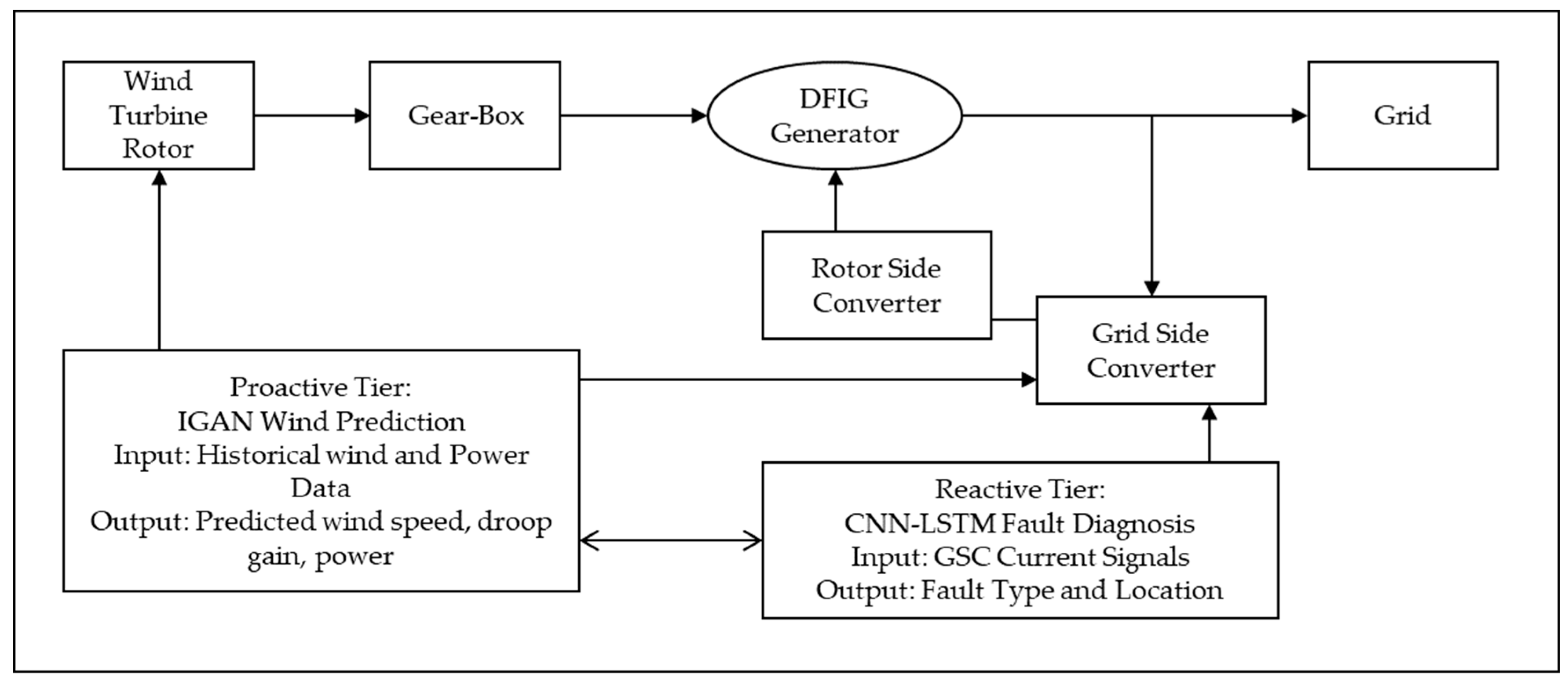
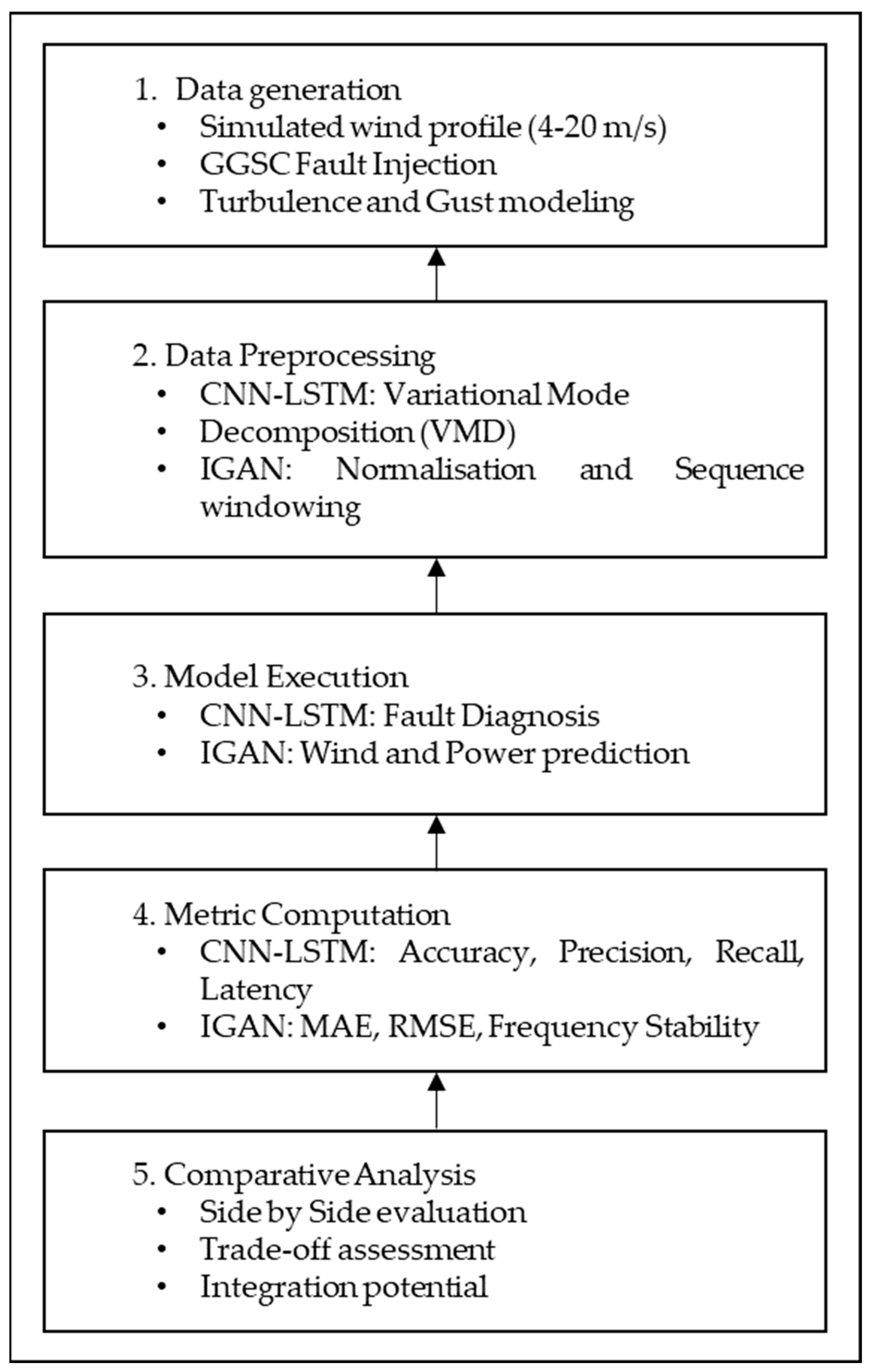
By analyzing Figure 1 and Figure 2 in conjunction, the authors determined that Figure 1 illustrates the overarching functional architecture and integration points of the two-tier AI system. Conversely, Figure 2 delineates the experimental pipeline that guarantees equitable and repeatable evaluation under uniform operational settings.

Figure 1 represents the enhanced high-level system architecture illustrating the integration of a two-tier AI control framework within a DFIG-based grid-connected wind turbine system. The proactive tier, implemented via the IGAN, forecasts short-term wind speed, active power, and droop gain values from historical wind and power data. The predictive module enables anticipatory adjustments to the droop control loop for improved frequency stability. The reactive tier, implemented via the CNN-LSTM fault diagnosis model, processes real-time GSC current signals to detect and classify IGBT faults, facilitating rapid fault isolation and system protection. Both tiers operate in a unified operational environment, sharing identical wind profiles, system parameters, and simulation configurations. This integrated design ensures a coherent predictive–diagnostic synergy for enhanced reliability and resilience in DFIG wind energy conversion systems.

Figure 2 represents the unified assessment and comparison pipeline for benchmarking the CNN-LSTM fault diagnosis system and the IGAN wind prediction framework in a DFIG-based wind turbine environment. The modeling scenario uses a common wind profile for all experiments, time-varying wind between 4 and 20 m s⁻¹ with turbulence and gusts defined by IEC 61400-1 [27] scripts, so that diagnostic (CNN-LSTM) and predictive (IGAN) models are exercised under identical external forcing. Controlled GSC IGBT faults are injected within 3–6 s of each run to test diagnostic responsiveness, while the same runs provide wind, power, and frequency series for prediction. Simulation settings are fixed across trials (step 20 µs, total 60 s, fixed-step ode4, logging 5 kHz), ensuring reproducibility and fair timing comparisons. Figure 2 delineates the modeling scenario, encompassing the actual wind farm, including the wind profile and site signals, disturbance and fault scripting, SCADA alignment, as well as fairness and comparability, all elaborated in next subsections.

Modeling situation:

The modeling configuration represents a grid-integrated DFIG wind turbine operated under a single, shared simulation environment so that both the diagnostic and predictive pipelines experience identical wind excitation, plant parameters, and grid conditions. This design eliminates confounding from mismatched setups and focuses the comparison on model capability rather than scenario differences.

Wind profile and site signals:

Wind speed at hub height (80 m), active power output, and grid frequency deviation (Δf) are the principal operational signals. The wind input follows a time-varying 4–20 m s⁻¹ trajectory with superimposed turbulence and gusts specified to IEC 61400-1; these scripts generate gradual day-to-day-like variations, high turbulence bursts, and step-type changes to probe short horizon predictability and controller robustness. These same runs provide the standardized input sequences used by IGAN (windowing 50 input steps → 10 forecast steps).

Plant and simulation settings:

The DFIG system is realized in MATLAB/Simulink with fixed parameters across all trials (electrical, mechanical, and control settings) and identical compute and logging budgets; signals are recorded at 5 kHz, with solver step 20 µs for 60 s per scenario. These constants ensure that inference latency and throughput measurements are comparable across the two pipelines.

Disturbance and fault scripting:

To evaluate reactive protection, IGBT open/short-circuit conditions in the GSC are injected deterministically between 3 and 6 s of each simulation; converter currents are sampled synchronously with the logging rate and pre-processed (VMD) for CNN-LSTM. In parallel, the predictive stream collects wind, power, and frequency traces from the same runs, ensuring one-to-one alignment of diagnostic events and predictive forecasts.

SCADA alignment:

The chosen variables, wind speed, rotor/electrical power, and frequency, mirror common SCADA channels in commercial turbines, supporting operational realism and facilitating eventual field transfer of the analytics.

Fairness and comparability:

Both pipelines use the same simulation outputs streamed into MATLAB for inference, with fixed random seeds and aligned decision horizons to maintain temporal comparability; this yields a like-for-like basis for accuracy and latency, and supports downstream system-level metrics (frequency-deviation reduction, power-regulation error) under identical conditions.

The pipeline standardizes experimental conditions by employing identical wind profiles, system parameters, and grid disturbance scenarios. The process comprises five stages:

• Data Generation: simulating wind profiles (4–20 m/s), injecting GSC faults, and modeling turbulence and gusts.
• Data Pre-processing: applying VMD decomposition for CNN-LSTM inputs, and normalization plus sequence windowing for IGAN inputs.
• Model Execution: running both models under identical simulation conditions.
• Metric computation: using accuracy, precision, recall, and latency for CNN-LSTM, and MAE, RMSE, and frequency stability for IGAN.
• Comparative analysis: side-by-side assessment to assess trade-offs and integration potential.

This unified framework ensures a fair, reproducible, and comprehensive assessment of both reactive and proactive AI-based control strategies for smart wind farms. Together, these figures provide a comprehensive view of the system-level integration and evaluation methodology underpinning the comparative study.

2.1. DFIG Wind Turbine System Simulation

The authors employed a standard grid-integrated DFIG wind energy conversion system in both the CNN-LSTM fault diagnosis and the Incremental GAN predictive control studies to ensure a consistent evaluation framework. This shared simulation environment allowed both models to be assessed under identical operational, environmental, and computational conditions, eliminating discrepancies arising from different experimental setups. The system was modeled and simulated in MATLAB/Simulink to reflect the dynamic behavior of a real-world wind farm [4,5].

2.1.1. System Overview

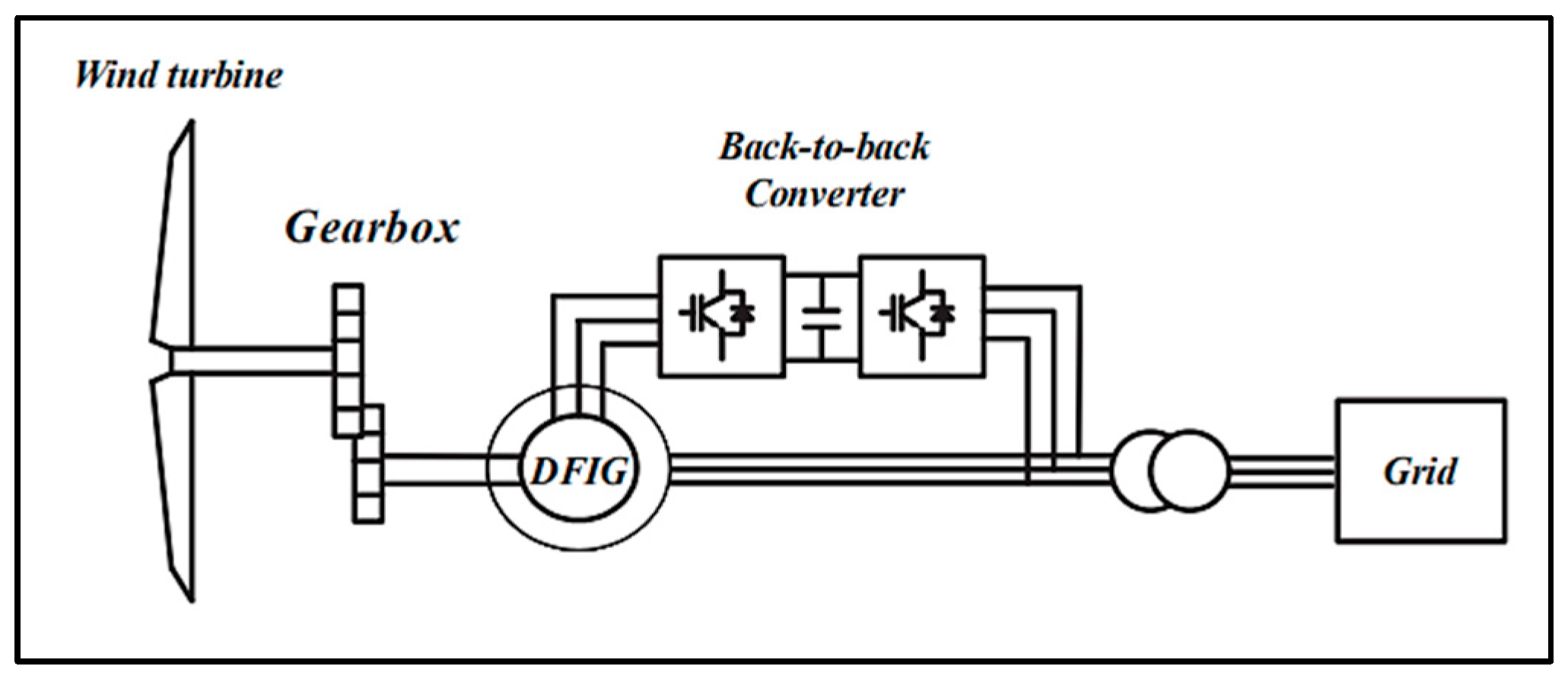
The DFIG wind energy conversion system consists of the following major subsystems. Figure 3 illustrates the DFIG-based wind energy system, with the stator directly connected to the grid and the rotor linked via back-to-back converters. Before developing a nonlinear controller, researchers must derive the nonlinear mathematical models of the RSC and GSC, which the following subsections.

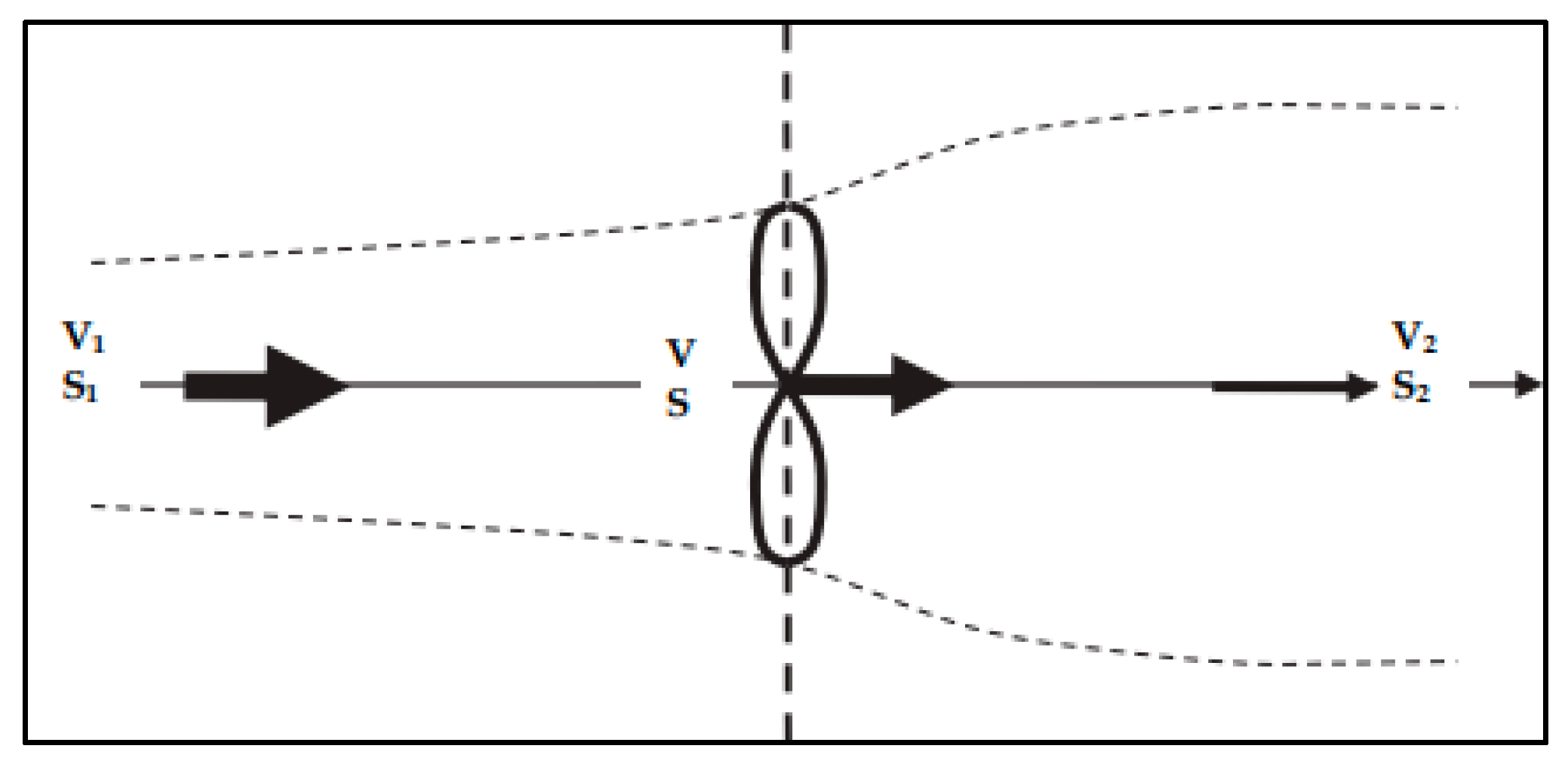
Considering the ideal wind rotor at rest in a fluid atmosphere, as shown in Figure 4 [28], Betz demonstrated that, for an ideal wind rotor in incompressible flow, the reduction in wind speed from upstream (V₁) to downstream (V₂), following mass conservation principles, limits the maximum extractable power. In this analysis, the wind speed (V₂) is explicitly defined as the velocity immediately behind the rotor at the rotor plane, capturing the first stage of wake formation. This distinction is crucial, as it represents the effective velocity interacting with the rotor’s aerodynamic surfaces and forms the basis for calculating extracted mechanical power before the far-wake velocity is established. The aerodynamic model, as shown in Figure 4, captures the conversion of wind kinetic energy into mechanical shaft power, with the tip-speed ratio and pitch angle dynamically adjusted based on wind conditions. The conservation of mass equation is:

$$m=\rho S_1{V}_1=\rho S_2{V}_2=constant$$

(1)

The power extracted by the rotor $P_r$:

$$P_r=\rho S{V}^2\left(V_1-V_2\right)={\displaystyle \frac{1}{2}}\rho SV\left(V_1-V_2\right)\left(V_1+V_2\right)$$

(2)

Ideal turbine power extraction P_m with $V_2={\displaystyle \raisebox{1ex}{$1$}\!\left/ \!\raisebox{-1ex}{$3$}\right.}{V}_1$ [28]:

$$P_m=P_{upwind}-P_{downwind}$$

(3)

Wind power as a rate of change in kinetic energy:

$$P_w={\displaystyle \frac{\frac{1}{2}m{V}_1^2-\frac{1}{2}m{V}_2^2}{∆t}}={\displaystyle \frac{1}{2}}\dot{m}\left(V_1^2-V_2^2\right)={\displaystyle \frac{1}{2}}\rho SV\left(V_1-V_2\right)\left(V_1+V_2\right)$$

(4)

And, therefore, the coefficient of power can be computed by:

$$C_p={\displaystyle \frac{Power extracted by the rotor}{Total power of the wind stream}}={\displaystyle \frac{\frac{1}{4}\rho SV{\left(V_1\right)}^2-{\left(V_2\right)}^2\left(V_1+V_2\right)}{\frac{1}{2}\rho S{V}^3}}$$

(5)

$$C_{p\_maxopt}=59.26\%$$

where $\rho$ is the air density, S is the swept area, and $C_{p\_maxopt}$ is known as the Betz optimization limit, which specifies the maximum amount of wind energy that may be transformed into rotational energy by the ideal wind turbine.

The turbine is mechanically coupled to the DFIG rotor via a low-speed shaft and gearbox, as shown in Figure 3. The DFIG operates in sub-synchronous and super-synchronous modes, allowing bidirectional rotor power flow between the rotor windings and the grid. The formula for the tip-speed ratio λ is expressed as follows:

$$\lambda ={\displaystyle \frac{{\omega }_{t}r}{V}}$$

(6)

The aerodynamic torque $T_r$ generated within the wind turbine with a gear ratio G, and the angular speed ${\omega }_t$, is expressed as follows, underlining its significance in the system’s overall performance [29]:

$$P={\displaystyle \frac{1}{2}}\rho C_{p\_max}S{V}_1^3$$

(7)

$$T_r={\displaystyle \frac{T_t{\omega }_t}{G}}={\displaystyle \frac{{\omega }_r}{G}}$$

(8)

By equating Equations (6)–(8), which represent the reference rotor speed ${\omega }_{r-ref}$ [29]:

$${\omega }_{r-ref}={\displaystyle \frac{{\lambda }_{opt}{G}_v}{R}}$$

(9)

$$P_{grid-ref}={\displaystyle \frac{1}{2}}\eta \rho r^2{C}_{{P-max}^{V^3}}$$

(10)

where η is denoted as the wind turbine efficiency.

2.1.2. Operation of the DFIG System and Control of Converters

The DFIG operates as a variable-speed wind energy conversion system in which the stator is directly connected to the grid while the rotor is interfaced through back-to-back voltage source converters. This configuration allows bidirectional energy flow between the rotor and the grid, enabling efficient operation in both sub-synchronous and super-synchronous modes. In sub-synchronous operation, part of the power is absorbed from the grid to the rotor circuit, whereas in super-synchronous operation, the rotor injects additional power back into the grid. Owing to this arrangement, only a fraction of the rated power (typically 20–30%) passes through the converters, thereby reducing the cost and losses compared to full-scale converter systems.

The converter system is composed of two stages: the RSC and the GSC, interconnected by a DC-link capacitor. The RSC plays a crucial role in controlling rotor currents, thereby enabling the independent regulation of active and reactive power exchanged with the grid. Through vector control techniques, the RSC decouples torque and flux control, ensuring an effective response to wind speed variations and system disturbances. In parallel, the GSC is responsible for maintaining DC-link voltage stability and for managing reactive power support at the grid interface. It employs current control strategies to regulate power exchange with the grid, ensuring compliance with grid codes and enhancing system stability during faults.

The control framework of the DFIG therefore extends beyond conventional PI regulators and vector control to incorporate advanced predictive and diagnostic intelligence. In this study, the CNN-LSTM diagnostic model is integrated with the GSC to provide rapid detection and localization of Grid Side Converter faults, thus preventing DC-link instability and ensuring uninterrupted power exchange. Meanwhile, the Incremental GAN-based predictive model is linked to the RSC, where accurate wind speed forecasting supports adaptive droop gain control and enhances primary frequency stability. By aligning AI-based control layers with the physical energy flow of the DFIG system, the proposed framework not only strengthens operational reliability but also addresses the practical challenges of fault tolerance and grid-supportive behavior in renewable energy integration.

2.1.3. Rotor Side Converter (RSC)

This subsection describes the speed controller and the d-q axis current controller.

Speed Controller

The phrase rotor angular speed ${\omega }_r$, in terms of generator speed ${\Omega }_r$, is written like:

$${\omega }_r=P{\Omega }_r$$

(11)

The rotor aerodynamic torque-speed ($T_r$ − ${\mathsf{\Omega }}_{\mathrm{r}}$). The relationship, sometimes known as the DFIG mechanical equation, is as follows [29]:

$$J{\displaystyle \frac{d}{dt}}{\Omega }_r=T_{em}-T_r-f_r{\Omega }_r$$

(12)

where the phrase electromagnetic torque $T_{em}$ in terms of rotor d-q axis fluxes ${\phi }_{ds}$, and ${\phi }_{qs}$, is written as [29]:

$$T_{em}=P{\displaystyle \frac{L_m}{L_s}}\left({\phi }_{qs}{I}_{dr}-{\phi }_{ds}{I}_{qr}\right)-T_r-f_r{\Omega }_r$$

(13)

Taking into consideration the relationship below to simplify the above expression:

$${\phi }_{ds}={\phi }_s, {\phi }_{qs}=0$$

(14)

The expression that results from combining Equations (13) and (14) is as follows:

$$T_{em}=P{\displaystyle \frac{L_m{V}_s}{{{\omega }_{s}L}_s}}{I}_{qr}$$

(15)

The expression for the d/q stator voltage vectors under constant stator flux and per-phase resistance is as follows [29]:

$$V_{ds}=0, V_{qs}=V_s={\omega }_s{\phi }_s$$

(16)

The d/q voltages in the rotor axis $V_{dr}$, $V_{qr}$ and stator side active-reactive powers $P_s$, $Q_s$, are expressed in terms of rotor current I_r as follows [30]:

$$V_{dr}=R_r\ast I_{dr}+\sigma L_r{\displaystyle \frac{d}{dt}}{I}_{dr}-\sigma L_{r}s{\omega }_s{I}_{qr}$$

(17)

$$V_{qr}=R_r\ast I_{qr}+\sigma L_r{\displaystyle \frac{d}{dt}}{I}_{qr}-\sigma s{\omega }_s{I}_{dr}+s{\displaystyle \frac{L_m{V}_s}{L_s}}$$

(18)

$$P_s=-{\displaystyle \frac{L_m{V}_s}{L_s}}{I}_{qr}$$

(19)

$$Q_s={\displaystyle \frac{V_s^2}{{\omega }_s{L}_s}}-{\displaystyle \frac{L_m{V}_s}{L_s}}{I}_{dr}$$

(20)

where σ and s are defined as follows:

$$\sigma =1-{\displaystyle \frac{L_m}{L_r{L}_s}}, \mathrm{and} s={\displaystyle \frac{{\omega }_s-{\omega }_r}{{\omega }_s}}$$

(21)

Here, s stands for the DFIG slip. The equations mentioned above describe the nonlinear system model as follows:

$$\dot{X}=A\left(x\right)+B\left(u\right)=a\left(x\right)+\Delta a+bu+\Delta bu$$

(22)

$$\dot{X}=A\left(x\right)+B\left(u\right)=a\left(x\right)+bu+\mathrm{d}\left(t\right)$$

(23)

In this case, $u=\left[u_1,u_2\right]={\left[V_{dr},V_{qr}\right]}^T$, and $X={\left[I_{dr},I_{qr}\right]}^T$, a and b represent the best approximation (nominal model) of A and B, respectively; ∆a and ∆bu denote plant and input vector uncertainties, whereas $d=\Delta \mathrm{a}+\Delta bu={\left[d_{I_d},d_{I_q}\right]}^T$ is the system model’s unknown lumped uncertainty.

The derivation process begins with the development of the speed controller, which is rooted in the dynamic model. The pulse width modulation controller is used to control RSC and GSC. This dynamic model in “(33)” is then reformulated and expressed as follows [29]:

$${\displaystyle \frac{d}{dt}}{\Omega }_r={\displaystyle \frac{T_{em}}{J}}+d_1$$

(24)

In this context, we introduce a key element known as the lumped uncertainty term, denoted as $d_1$. The equation precisely represents this uncertainty term [29]:

$$d_1=-{\displaystyle \frac{T_r}{J}}-{\displaystyle \frac{f_r{\mathsf{\Omega }}_r}{J}}$$

(25)

Now, within the context of “(24)”, it is important to note that $T_{em}$, stands for the control input, while J represents the moment of inertia. Furthermore, the speed tracking error $e_1$ is formally defined in the following manner [29]:

$$e_1={\mathsf{\Omega }}_r-{\mathsf{\Omega }}_{r-ref}$$

(26)

The time derivative of $h_1$ can be expressed $\dot{e_1}=\dot{{\mathsf{\Omega }}_r}-\dot{{\mathsf{\Omega }}_{r-ref}}$. By substituting Equation (24) in $\dot{e_1},$ obtains a modified expression as follows [29]:

$$\dot{e_1}={\displaystyle \frac{T_{em}}{J}}+{\mathrm{d}}_1-\dot{{\mathsf{\Omega }}_{r-ref}}$$

(27)

To formulate the speed controller, we opt for a fractional-order sliding surface, expressed as follows [29]:

$$S_1=c_1{O}^{-\alpha }{e}_1+c_2\int \dot{e_1}$$

(28)

In this context, the variables $c_1$, and $c_2$ stand as design constants for the sliding surface. By applying the fractional operator $O^{\alpha }$ to Equation (28) derives the following expression [29]:

$$O^{\alpha }{S}_1=c_1{e}_1+ c_2{O}^{\alpha -1}\dot{e_1}$$

(29)

Upon combining Equation (28) with Equation (29), we obtain the modified relation as follows:

$$O^{\alpha }{S}_1=c{e}_1+ c_2{O}^{\alpha -1}\left[{\displaystyle \frac{T_{em}}{J}}+d_1-{\dot{\mathsf{\Omega }}}_{r-ref}\right]$$

(30)

From Equation (30), we derive the speed controller as follows [29]:

$$\left\{\begin{array}{c}{T}_{em}=T_{em-eq}+T_{em-s}\\ T_{em-eq}=J\left({\dot{\mathsf{\Omega }}}_{r-ref}-O^{1-\alpha }{\displaystyle \frac{c_1}{c_2}}{e}_1\right)\\ T_{em-s}=J\left(-{\displaystyle \frac{k_{r1}}{c_2}}{O}^{1-\alpha }sgn\left(S_1\right)\right)\end{array}\right.$$

(31)

Equation (31) introduces $k_{r1}$ as the discontinuous gain parameter of the controller. Notably, within the term $T_{em-s}$, there is a fractional derivative that considers the magnitude $\left(O^{1-\alpha }\right)$. This specific inclusion plays a pivotal role in dampening the chattering phenomena, ultimately contributing to improved overall control performance.

d-q Axis Current Control

We first express the active power P and reactive power Q as follows to derive the d- and q-axis current controllers:

$$I_{qr-ref}={\displaystyle \frac{{\omega }_s{L}_s}{P{L}_m{V}_s}}{T}_{em-ref}$$

(32)

$$Q_{ref}={\displaystyle \frac{V_s^2}{{\omega }_s{L}_s}}-{\displaystyle \frac{L_m{V}_s}{L_s}}{I}_{dr-ref}$$

(33)

with $Q_{ref}=0$, we express the reference d-axis current as:

$$I_{dr-ref}={\displaystyle \frac{V_s}{L_m{\omega }_s}}{T}_{em-ref}$$

(34)

The following defines the current tracking faults on the d and q axes:

$$e_2={\left[\begin{array}{cc}{e_I}_d & {e_I}_q \end{array}\right]}^T={\left[\begin{array}{cc}{I}_{dr}-I_{dr-ref} & I_{qr}-I_{qr-ref} \end{array}\right]}^T$$

(35)

$$\dot{{\dot{e}}_2=\dot{x}-{\dot{x}}_{ref}=a\left(x\right)+bu+d-{\dot{x}}_{ref}}$$

(36)

The fractional order sliding surface S, with c₃; c₄; c₅; and c₆ are the design parameters:

$$S=\left[\begin{array}{c}{S}_2\\ S_3\end{array}\right]=\left[\begin{array}{c}{c}_3{O}^{-\alpha }{e_I}_d+c_4\int {{\dot{e}}_I}_d\\ c_5{O}^{-\alpha }{e_I}_q+c_6\int {{\dot{e}}_I}_q\end{array}\right]$$

(37)

By applying the fractional operator O^a to Equation (37), the resultant expression:

$$O^{\alpha }S=\left[\begin{array}{c}{O^{\alpha }S}_2\\ {O^{\alpha }S}_3\end{array}\right]=\left[\begin{array}{c}{c}_3{e_I}_d+c_4{O}^{\alpha -1}{{\dot{e}}_I}_d\\ c_5{e_I}_q+c_6{O}^{\alpha -1}{{\dot{e}}_I}_q\end{array}\right]$$

(38)

Hence, the equivalent control terms

$$u_{eq}=\left[\begin{array}{c}{u}_{eq1}\\ u_{eq2}\end{array}\right]=\left[\begin{array}{c}{b}^{-1}\left(-a\left(x\right)+{\dot{I}}_{d-ref}-{\displaystyle \frac{c_3{O}^{1-\alpha }{e}_{I_d}}{c_4}}\right)\\ b^{-1}\left(-a\left(x\right)+{\dot{I}}_{qr-ref}-{\displaystyle \frac{c_5{O}^{1-\alpha }{e}_{I_q}}{c_6}}\right)\end{array}\right]$$

(39)

$$u_s=\left[\begin{array}{c}{u}_{s1}\\ u_{s2}\end{array}\right]=\left[\begin{array}{c}{b}^{-1}\left[{\displaystyle \frac{{-k}_{r2}{O}^{1-\alpha }sgn\left(S_2\right)}{c_4}}\right]\\ b^{-1}\left[{\displaystyle \frac{{-k}_{r3}{O}^{1-\alpha }sgn\left(S_3\right)}{c_6}}\right]\end{array}\right]$$

(40)

We can achieve the sliding condition by assigning values to the setting $k_r=\left[\begin{array}{cc}{k}_{r2}& k_{r3}\end{array}\right]>d_{max}$ where $d_{max}$ denotes the maximum limit of the disturbance and assume that this limit is known. The RSC is responsible for controlling rotor currents to regulate the active power (P) and reactive power (Q) output of the DFIG. We applied a vector control strategy in the d-q-0 synchronous reference frame to decouple the active and reactive power control. The control strategy enables maximum power point tracking (MPPT) at low wind speeds and pitch-controlled operation at high wind speeds.

2.1.4. DC Link Voltage Formulation and Grid Side Converter (GSC)

Throughout the control operation, the DC link capacitor connected between the RSC and GSC converters maintains the DC link voltage. Without changing the DC link voltage, the GSC converter side controls the active power (P) and reactive power (Q). The authors accomplished this by applying a traditional vector control method, such as lining up the reference frame with the grid or stator voltage vector. Consequently, $V_d=V_s$, and $V_q=0$.

As a result, the authors used the following formulas for P and Q.

$$P_s=\left({\displaystyle \frac{3}{2}}\right)\left(V_{ds}{I}_{ds}+V_{qs}{I}_{qs}\right)={\displaystyle \frac{3}{2}} \left(V_{ds}{I}_{ds}\right)$$

(41)

$$Q_s=\left({\displaystyle \frac{3}{2}}\right)\left(V_{ds}{I}_{ds}-V_{ds}{I}_{qs}\right)=-{\displaystyle \frac{3}{2}} \left(V_{ds}{I}_{ds}\right)$$

(42)

The ratio of the current component $I_d$ to active power and current component $I_q$ to reactive power flowing between the GSC converter and the grid is represented by Equations (41) and (42).

$$E{I}_{os}={\displaystyle \frac{3}{2}}{V}_d{I}_d$$

(43)

where $E$ represents the DC link voltage, $I_{os}$ is the stator side, and $I_{or}$ is the rotor side DC link current. Additionally, the following shift in DC power equals the GSC converter-grid active power.

$$C{\displaystyle \frac{dE}{dt}}=I_{os}-I_{or}$$

(44)

Upon combining Equation (43) with Equation (44), the modified relation is obtained as follows:

$$\dot{E}={\displaystyle \frac{1}{C}}\left({\displaystyle \frac{3}{2E}}{V}_d{I}_d-I_{or}\right)$$

(45)

$$\dot{E}=g\left(x\right)I_d-{\displaystyle \frac{1}{C}}{I}_{or}$$

(46)

$$\dot{E}=\left(∆g\left(x\right)+g_o\left(x\right)\right)I_d-{\displaystyle \frac{1}{C}}{I}_{or}$$

(47)

$$\dot{E}=g_o\left(x\right)I_d-{\displaystyle \frac{1}{C}}{I}_{or}+d_E$$

(48)

Here $d_E=∆g\left(x\right)I_d$, represents an uncertainty term.

To maintain a constant DC link voltage, the mathematical model calculates the error as the difference between the reference DC voltage and the actual DC link voltage, expressed as follows [29]:

$$e_E=E-E^{\ast }$$

(49)

The following equation expresses the time derivative of the error:

$${\dot{e}}_E=\dot{E}-{\dot{E}}^{\ast }$$

(50)

Upon substituting the expression for $\dot{E}$ into Equation (50), the resulting expanded expression is as follows [29]:

$${\dot{e}}_E=g_o\left(x\right)I_d-{\displaystyle \frac{1}{C}}{I}_{or}+d_E-{\dot{E}}^{\ast }$$

(51)

To regulate the DC link voltage effectively, we opt for a fractional calculus-based sliding surface described by Equation (52):

$$S_E=c_7{O}^{-\alpha }{e}_E+c_8\int {\dot{e}}_E$$

(52)

Upon applying the operator $O^{\alpha }$ to both sides of Equation (52), the resulting relation is as follows [29]:

$${O^{\alpha }S}_E=c_7{e}_E+c_8{O}^{\alpha -1}{\dot{e}}_E$$

(53)

By combining Equation (52) with Equation (53), we obtain the following expanded relation:

$${O^{\alpha }S}_E=c_7{e}_E+c_8{O}^{\alpha -1}{\dot{e}}_E\left(g_o\left(x\right)I_d-{\displaystyle \frac{1}{C}}{I}_{or}+d_E-{\dot{E}}^{\ast }\right)$$

(54)

Utilizing Equation (54), the control law can be defined as follows [29]:

$$\left\{\begin{array}{c}{I}_d=I_{deq}+I_{ds}\\ I_{deq}={\displaystyle \frac{1}{go\left(x\right)}}\left\{{\dot{E}}^{\ast }+{\displaystyle \frac{1}{c_7}}{I}_{or}-{\displaystyle \frac{c_7}{c_8}}{O}^{1-\alpha }\left(e_E\right)\right\}\\ I_{ds}={\displaystyle \frac{1}{go\left(x\right)}}\left(-{\displaystyle \frac{k_{r4}}{c_8}}{O}^{1-\alpha }\left(sgn\left(S_E\right)\right)\right)\end{array}\right.$$

(55)

In Equation (55), $c_7$ and $c_8$ serve as the design parameters while $k_{r4}$ represents the discontinuous switching gain. This formulation captures the key components of Equation (55), allowing for precise control system design and parameter tuning.

In the fault diagnosis context, the GSC IGBT modules are critical components where open-circuit or short-circuit faults can cause operational instability. A DC link capacitor interconnects the RSC and GSC and smooths the power exchange between the rotor and the grid. Control loops in both converters operate at high sampling rates (5–10 kHz) to respond quickly to transient events. The converter control system is implemented in MATLAB/Simulink using discrete-time PI controllers, PWM switching logic, and gating signals for the IGBTs.

2.1.5. Adaptive Droop Control for Frequency Regulation

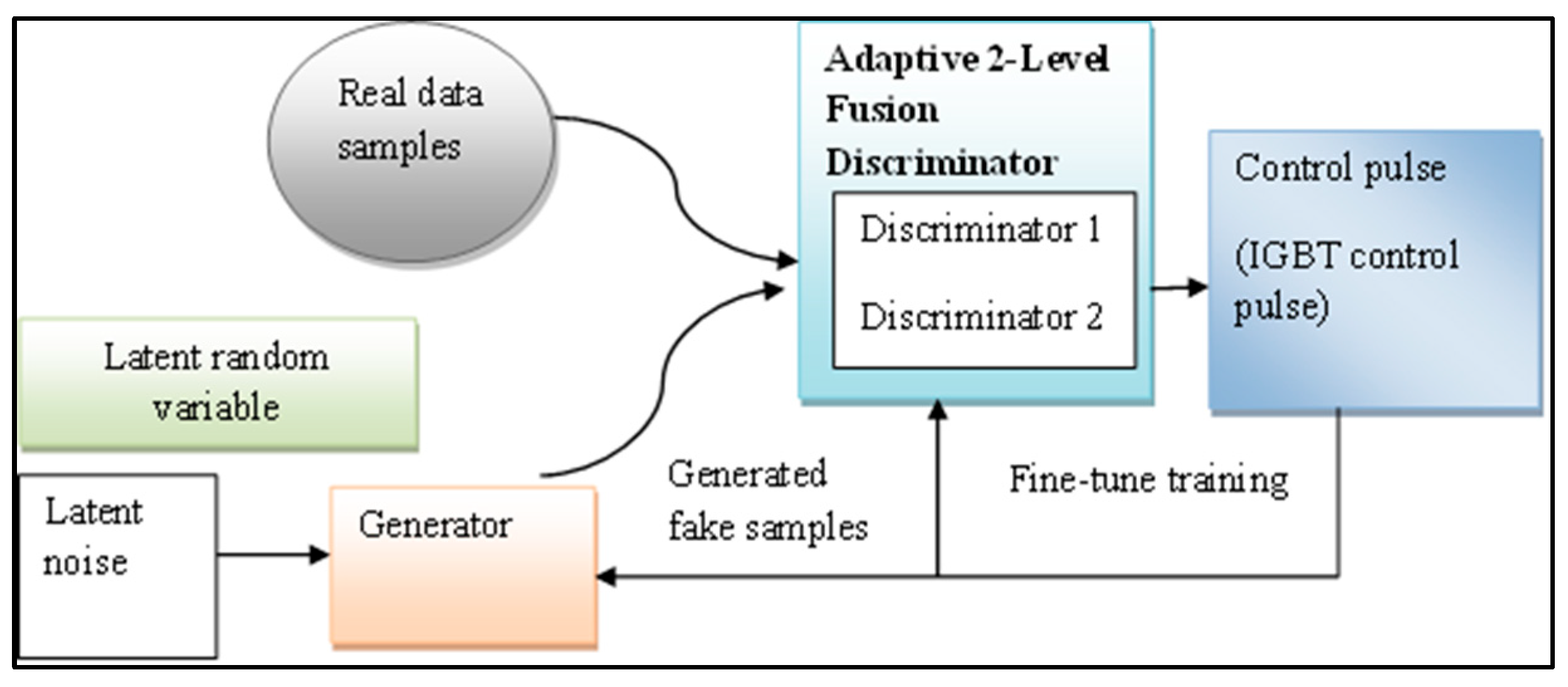
As shown in Figure 5, the authors in [4] explain how the GAN is applied to improve wind energy generation and management, highlighting the novelty of the discriminator, adaptive two-level fusion, and the integration of a self-attention mechanism. The droop control mechanism adjusts the active power output proportionally to frequency deviations in the grid. The droop gain parameter regulates the speed at which a generator adjusts its output voltage and frequency in response to changes in load or generation, contributing to grid stability by redistributing the load among multiple wind farm generators. The authors depict each DFIG-WT as a voltage source connected to a shared bus through a line impedance Z and express the power transfer from the wind unit to the Point of Common Coupling (PCC) bus as follows [31]:

$$S_A=P_A+j{Q}_A=U_{A^{e^{j{\delta }_p}}}\left({\displaystyle \frac{U_A{e}^{-j{\delta }_p}- U_B }{Z{e}^{-j\gamma }}}\right)$$

(56)

$$S_A={\displaystyle \frac{U_A^2}{Z}}{e}^{j\gamma }-{\displaystyle \frac{{U_{A}U}_B}{Z}}{e}^{j\left(\gamma +{\delta }_p\right)}$$

(57)

In this context, $S_A$ and $S_B$ correspond to the magnitudes of the wind unit and PCC bus voltages, while Z and γ, respectively, signify the magnitude and phase angle of the line impedance. Furthermore, ${Ze}^{j\gamma }=R+jX$, and ${\delta }_p$, which characterizes the power angle. To establish the voltage difference, the model employs $\left(\Delta \mathrm{U}=U_A-U_B\right)$ [31].

$$\Delta U={\displaystyle \raisebox{1ex}{$\left(R{P}_A+X{Q}_A\right)$}\!\left/ \!\raisebox{-1ex}{$U_A$}\right.}$$

(58)

$${\delta }_p={\displaystyle \raisebox{1ex}{$\left(X{P}_A-R{Q}_A\right)$}\!\left/ \!\raisebox{-1ex}{$U_A{U}_B$}\right.}$$

(59)

Equations (58) and (59) illustrate the decoupling of $\left(P-Q\right)$ from each other solely through ${\delta }_p- \Delta \mathrm{U}$, but this scenario holds only in an ideal case, specifically, in cases where there is either pure inductance $\left(X=0\right)$ or pure resistance $\left(R=0\right)$. When applied $\left(R=0\right)$ to Equations (58) and (59), the following outcome emerges [31]:

$$P_A=U_A{U}_B{\delta }_p/X$$

(60)

$$Q_A=U_A\Delta U/X$$

(61)

Under these conditions, the authors deploy the conventional droop-sharing scheme to control and regulate the active and reactive power output of the wind turbine generator unit as follows [31]:

$$f=f_o-mP$$

(62)

$$U=U_o-nQ$$

(63)

Here $f_o$ and $U_o$ parameters are associated with the frequency and amplitude of the wind turbine generator unit voltage at no load (set points). We describe the droop coefficients for these parameters as follows: m denotes the frequency droop coefficient, and n denotes the voltage droop coefficient [31].

$$m=\Delta f/P_n$$

(64)

$$n=\Delta \mathrm{U}/Q_n$$

(65)

In this context, $P_n$ represents the nominal active power, and $Q_n$, represents the nominal reactive power of the wind unit. Usually, permissible deviations of up to 2% for $\Delta f$ and 5% for $\Delta \mathrm{U}\mathrm{e}\mathrm{x}\mathrm{i}\mathrm{s}\mathrm{t}$. It is standard practice to maintain $\Delta f$ and $\Delta \mathrm{U}$ as equal values across all units.

$$\Delta f=m{P}_{n1}=m_2{P}_{n2}=\dots \dots \dots =m_j{P}_{nj}$$

(66)

$$\Delta U=n_1{Q}_{n1}=n_2{Q}_{n2}=\dots \dots \dots =n_j{Q}_{nj}$$

(67)

Consequently, the coefficients exhibit an inverse relationship with nominal powers. Choosing the droop coefficients following Equations (66) and (67) guarantees that each unit contributes to power sharing in alignment with its designated nominal rating [31].

In the IGAN predictive control study [4], researchers dynamically updated the droop gain (K_p) based on predicted wind and power values, improving grid frequency stability during rapid wind changes. This control strategy ensures smooth power sharing among generators and mitigates oscillations.

2.1.6. Wind Speed Profile and Operating Conditions

The wind speed profile is a critical factor in evaluating the operational performance and control strategies of a DFIG-based wind energy conversion system, as it directly influences turbine aerodynamic efficiency, generator loading, and grid interaction. In this study, the authors simulated a wind profile to reflect realistic operating conditions, covering the full operational range of the turbine, from cut-in speed to rated speed and extending towards cut-out speed, while incorporating turbulence and gust effects to evaluate system robustness.

Wind Speed Range and Regimes

The operational wind speed range was set between 4 and 20 m/s, encompassing the three main regimes of wind turbine operation:

• Below rated (cut-in to rated speed)—From approximately 4 to 12 m/s, the turbine operates in maximum power point tracking (MPPT) mode, adjusting rotor speed to optimize the tip-speed ratio (λ) for maximum aerodynamic efficiency.
• Rated speed operation—Around 12 m/s to 15 m/s, the turbine output reaches its rated electrical power. Rotor speed is regulated, and blade pitch control begins to limit aerodynamic power to protect mechanical components.
• Near cut-out speed—At wind speeds above 15 m/s, pitch control actively limits rotor power to prevent overload. At 20–25 m/s, the turbine typically shuts down to avoid structural damage, but in the simulation, researchers modeled this region for control stress testing.

Wind Profile Modeling

The authors generated a wind profile using a combination of deterministic and stochastic components:

• Base Mean Wind Speed (V_avg): A slowly varying reference speed to simulate large-scale atmospheric changes.
• Turbulence Component (V_t): Generated using a stochastic process to represent short-term wind fluctuations typical in onshore and offshore environments.
• Gust Events (V_g): Modeled as step changes in wind speed over short durations to assess system transient response and stability.

The following definition specifies the overall wind profile:

$$V\left(t\right)=V_{avg}\left(t\right)+ V_t\left(t\right)+V_g\left(t\right)$$

(68)

where:

• $V_{avg}\left(t\right)$ represents gradual wind speed changes (e.g., due to diurnal cycles),
• $V_t\left(t\right)$ models high-frequency turbulence using Gaussian white noise filtered to match IEC 61400-1 standards,
• $V_g\left(t\right)$ introduces rapid gusts with a 5–10 s rise time.

Operational Impact

The wind variability serves multiple purposes in the simulation:

• For the CNN-LSTM fault diagnosis model [5], fluctuating wind speeds create varying load conditions, ensuring that current signal patterns used for fault detection represent realistic, non-stationary operating states.
• For the IGAN wind prediction model [4], realistic wind speed dynamics provide a challenging dataset for short-term forecasting, particularly in predicting gust-induced transients and adapting droop gain values for frequency regulation.

Relevance to System Evaluation

This controlled yet realistic wind profile ensures that:

• The authors tested the fault detection accuracy under dynamic aerodynamic loading rather than static conditions.
• The authors evaluated the wind prediction performance in complex, real-world operational scenarios that combine smooth variations, turbulence, and gusts.
• The comparative analysis between diagnostic and predictive models reflects actual operational stress conditions for a DFIG wind turbine.

The aerodynamic, mechanical, and electrical equations used in this work are drawn from well-established models of wind turbine and DFIG operation, serving as the physical foundation of this study rather than a novel theoretical contribution. The originality lies in systematically integrating these standardized models into a unified DFIG-based simulation with converter control and DL-driven diagnostic and predictive tools. This integration enables physically consistent benchmarking, ensuring that the comparative evaluation of DL models is both reliable and interpretable.

2.1.7. Simulation Parameters

We carefully selected the simulation parameters for the DFIG-based wind energy conversion system to replicate the electrical, mechanical, and aerodynamic characteristics of a utility-scale, grid-connected wind turbine while maintaining computational efficiency for repeated model execution in both fault diagnosis and wind prediction scenarios. These parameters are consistent across the CNN-LSTM fault detection [5] and Incremental GAN predictive control [4] studies to ensure a fair and controlled comparative evaluation.

Electrical System Parameters

The authors parameterized the electrical subsystem of the DFIG model as shown in

Table 1. Electrical system parameters.

Parameter	Value	Description
Rated Power	2 MW	Nominal output at rated wind speed
Stator Voltage	450 V	Line-to-line RMS, consistent with IEC grid connection standards
Rated Stator Frequency	50 Hz	Matches the grid frequency for synchronisation
DC Link Voltage	1200 V	Maintains power balance between RSC and GSC
Stator Resistance (Rs)	1.33 pu	Per-unit based on generator base values
Rotor Inductance (Rr)	0.06 pu	Impacts rotor current control
Stator Leakage Inductance	0.06 pu	Limits short-circuit currents
Magnetizing Inductance	3.5 pu	Determines flux linkage in the DFIG core

to reflect a commercially available 2 MW class wind turbine generator:

Mechanical and Aerodynamic Parameters

The authors selected the mechanical and aerodynamic properties to capture realistic turbine rotor dynamics and wind-to-power conversion characteristics.

Table 2. Mechanical and aerodynamic parameters.

Parameter	Value	Description
Rotor Diameter	80 m	Determines swept area for wind capture
Swept Area (A)	5026 m2	Matches commercial onshore turbine design
Hub Height	80 m	Converts low-speed rotor torque to high-speed generator rotation
Gearbox Ratio	1:90	Defines kinetic energy stored in a rotating mass
Inertia Constant (H)	4.5 s	Standard at sea level under IEC conditions
Air Density (ρ)	1.225 kg/m3	Optimal aerodynamic efficiency range
Tip-Speed Ratio (λ)	7–8	Near-Betz-limit aerodynamic efficiency
Power Coefficient (Cp)	0.48 (max)	Matches commercial onshore turbine design

illustrates the parameterization index.

Converter and Control Parameters

The authors modeled the RSC and GSC blocks with a back-to-back configuration and independent control loops.

Table 3. Converter and control parameters.

Parameter	Value	Description
PWM Switching Frequency	5 kHz	High enough for smooth current waveforms
Current Control Bandwidth	200 Hz	Enables fast dynamic response
PI Controller Gains (RSC)	Adaptive	Tuned for active/reactive power decoupling
PI Controller Gains (GSC)	Adaptive	Tuned for DC link voltage regulation
Droop Gain (Kp)	Adaptive	Updated dynamically in IGAN predictive control scenarios

illustrates the parameterization index of the modeled converters which were adopted from established benchmark models reported in [4] to maintain consistency with prior studies on DFIG wind turbine systems.

Simulation Configuration

The MATLAB/Simulink simulation was designed for high-resolution time-domain analysis.

Table 4. Simulation parameters.

Setting	Value
Simulation Step Size	20 μs
Total Simulation Time	60 s
Numerical Solver	Fixed-step, ode4 (Runge–Kutta)
Data Logging Frequency	5 kHz
Fault Injection Intervals	3–6 s

illustrates the parameterization index of the simulated parameters.

Operational Consistency Across Models

To ensure comparative integrity:

• Both CNN-LSTM and IGAN models used identical electrical, mechanical, and control parameters.
• The authors applied identical wind speed profiles 4 m/s to 20 m/s with turbulence to both models.
• The authors simulated the identical disturbance and fault conditions to test each model’s robustness.
• The authors logged the simulation outputs in a structured dataset for direct performance benchmarking.

Relevance to Evaluation

The choice of parameters ensures:

• Realistic turbine representation consistent with IEC 61400-1 standards [27].
• High-fidelity system dynamics for testing AI-based control and diagnostic algorithms.
• Reproducibility for future research comparisons and benchmarking.

2.2. Model Development and Contribution

The baseline model of the DFIG-based wind energy conversion system was developed using standard MATLAB/Simulink blocks for the generator, Rotor Side Converter, and Grid Side Converter. This ensured that the electrical and mechanical dynamics of the machine were represented according to widely accepted reference models. The novelty of this work lies in the adaptation and extension of this baseline framework by integrating advanced diagnostic and predictive deep learning models directly into the control loops. Specifically, the CNN-LSTM architecture was embedded within the Grid Side Converter to provide real-time fault detection and localization, while the Incremental GAN was coupled with the Rotor Side Converter to enhance adaptive control through wind speed forecasting. Furthermore, additional refinements in parameterization, energy flow analysis, and converter interaction were introduced to align the simulation environment with realistic operating conditions. This integration of AI-based models into a standard DFIG simulation platform represents the authors’ original contribution, enabling a more comprehensive performance evaluation than what is found in the conventional literature.

3. Overview of Experimental Framework

This study establishes a unified evaluation setting in which the CNN-LSTM diagnostic model for Grid Side Converter (GSC) IGBT faults and the Incremental GAN (IGAN) predictive model for wind attributes operate on the same DFIG Simulation. The framework’s purpose is to compare diagnostic accuracy and efficiency against predictive performance and adaptability using identical environmental conditions, system parameters, and common metrics such as accuracy, MAE, and inference time. 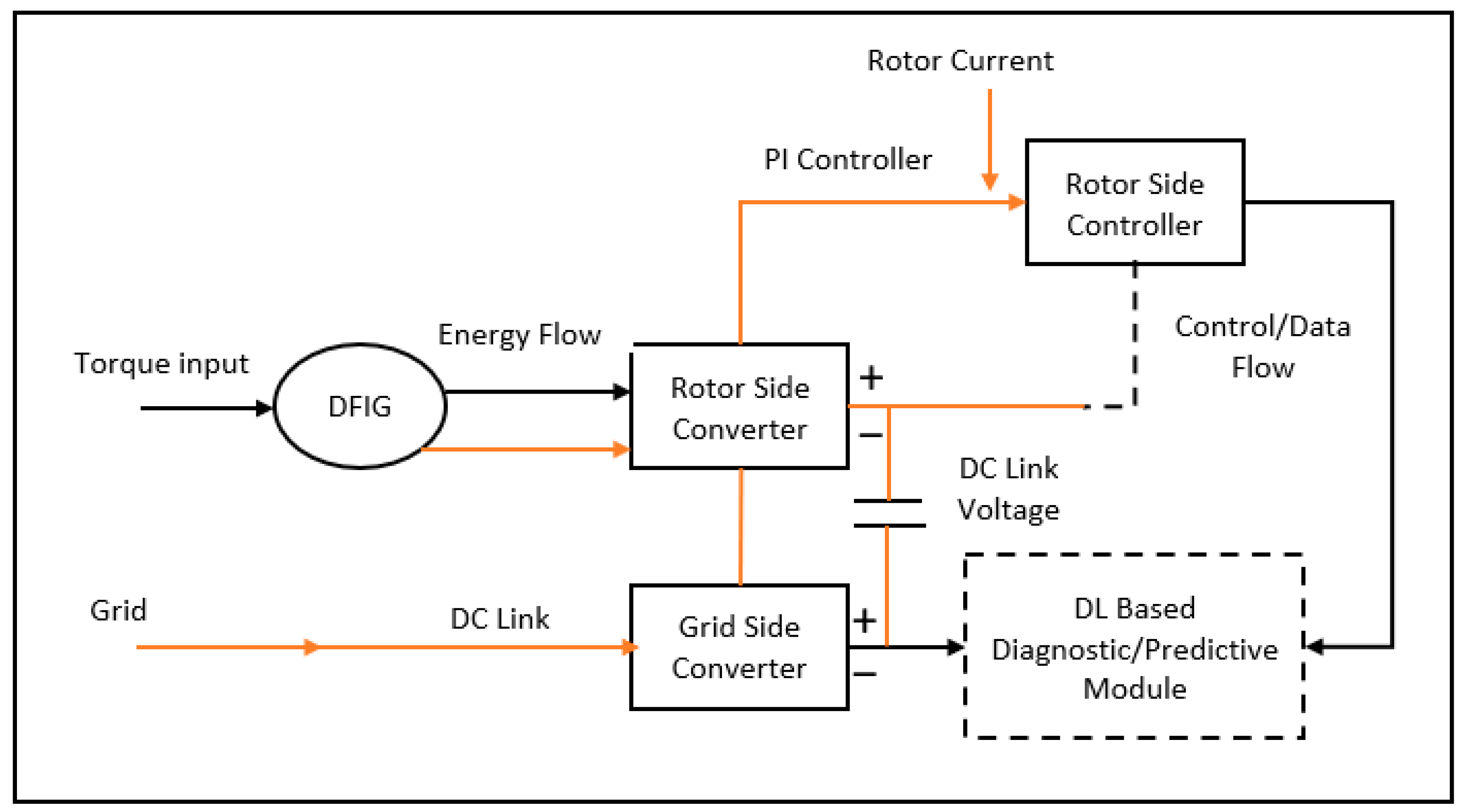Figure 6 depicts the integrated architecture in a grid-connected DFIG environment, which ensures that both models are assessed under equivalent operating scenarios for a fair comparison.

In Figure 6, the solid orange lines denote the flow of energy and electrical power within the system, while the black solid lines outline the system blocks and their functional interconnections. In contrast, the black dashed lines indicate control and data flow rather than physical energy transfer.

3.1. CNN-LSTM-Based Fault Diagnosis System

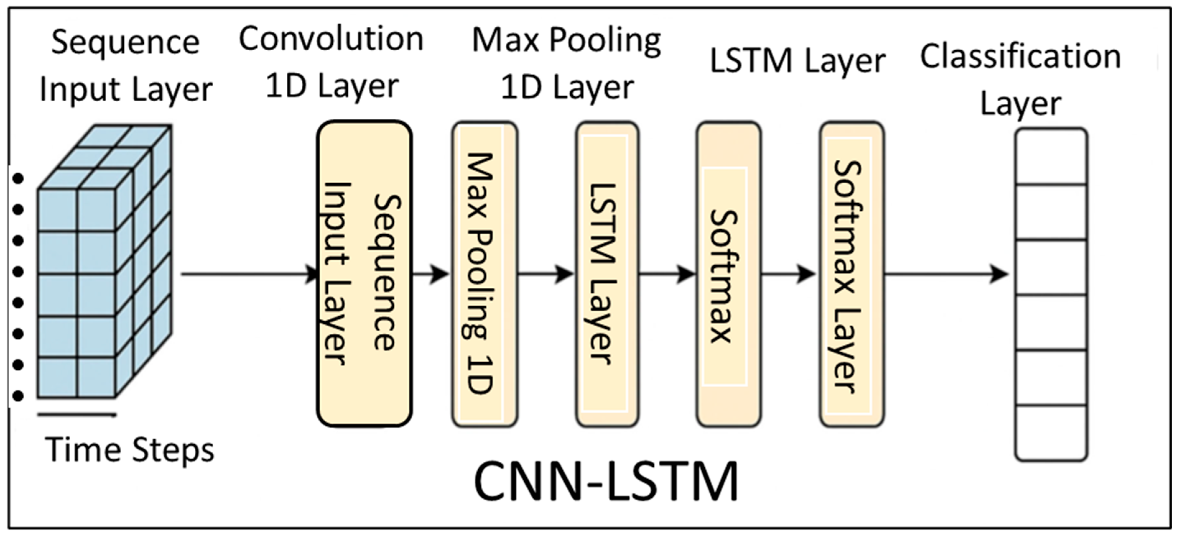
The CNN-LSTM system in [5] targets GSC IGBT fault detection and classification in a DFIG wind turbine subjected to varying wind and grid conditions [32,33]. The hybrid design combines convolutional layers for spatial feature extraction with LSTM layers for temporal sequence modeling, enabling the network to identify fault signatures embedded in time-series converter currents. The CNN-LSTM diagnostic framework shown in Figure 7 and developed by [5] follows the architecture previously validated in the literature and is integrated within the MATLAB/Simulink DFIG model so that data generation and model evaluation occur within the same physical simulation loop. This setup allows the classifier to exploit VMD-processed current signals and to report performance through accuracy and confusion analyses under realistic disturbances.

3.1.1. Fault Modeling and Dataset Generation

The dataset captures operational states dominated by converter behavior, including healthy operation and both open-circuit and short-circuit IGBT faults at single- and double-device levels. Faults are injected between 3 and 6 s of simulated time while wind speed varies from 4 to 20 m/s with turbulence, ensuring that the diagnostic model experiences a representative range of aerodynamics-to-electrical transients. Three-phase GSC output currents are sampled at 5 kHz and each simulated condition lasts 10 s, producing balanced episodes for supervised learning without resorting to hardware experiments.

3.1.2. Signal Pre-Processing Using Variational Mode Decomposition (VMD)

Since, the raw converter currents are non-stationary and noise-corrupted, the signals are decomposed by Variational Mode Decomposition (VMD) into a finite set of intrinsic mode functions. Lower-frequency modes preserve the harmonic distortions that reveal fault signatures while attenuating high-frequency switching noise; each mode is then mapped as a separate channel to the CNN, yielding a multi-channel representation that has been shown to isolate fault evidence more effectively than classical wavelets, as confirmed in [5].

3.1.3. CNN-LSTM Network Architecture

The network begins with convolutional layers (3 × 3 kernels with ReLU activations) and intermediate pooling to condense spatial features from the VMD channels before flattening to a vector representation. This vector feeds into stacked LSTM layers that capture long- and mid-range temporal dependencies; dropout regularization reduces overfitting. A fully connected output layer with softmax activation performs multi-class classification, covering ten fault classes plus the healthy state.

3.1.4. Training and Validation Setup

Data are split into training, validation, and test partitions at 70%, 20%, and 10%, respectively. Optimization uses Adam with a 0.001 learning rate and categorical cross-entropy loss, trained for up to 100 epochs with early stopping to prevent overfitting; robustness is further improved by injecting additive Gaussian noise 0.3–0.7 during training to reflect sensor and switching disturbances encountered in practice.

3.1.5. CNN-LSTM Model Performance Evaluation Metrics

Diagnostic performance is reported using classification accuracy, precision, recall, the F1-score, and class-wise confusion matrices. Implementation-level feasibility is addressed through execution time measurements, and robustness is quantified by tracking accuracy degradation under noisy inputs.

3.1.6. Role in Comparative Analysis

Within the overall framework, CNN-LSTM provides the reactive layer that identifies and isolates GSC faults in real time. Because both the diagnostic and predictive models share the same DFIG configuration, events flagged by the classifier can be temporally correlated with IGAN-predicted power fluctuations, enabling an integrated reliability narrative for wind farm operation.

3.2. Incremental GAN-Based Wind Prediction Framework

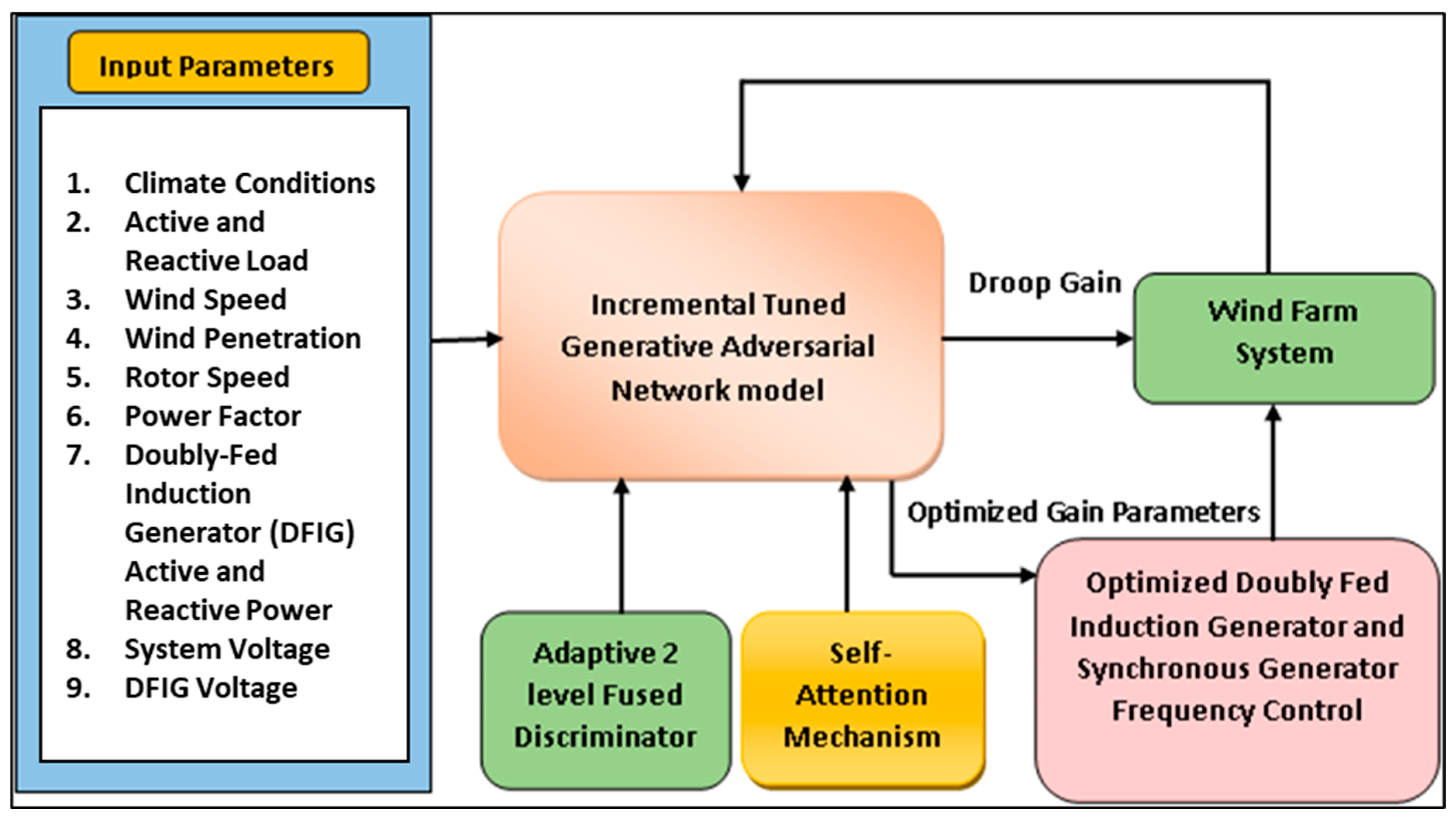
The IGAN component forecasts short-term wind speed, active power, and droop-gain trajectories in a grid-integrated DFIG system. By learning both global sequence structure and local temporal fluctuations from historical operating data, the predictor supports adaptive droop control that improves frequency stability and power sharing under rapidly changing wind conditions. The IGAN architecture shown in Figure 8 from the literature is implemented in the same MATLAB/Simulink DFIG environment used for the diagnostic workflow, ensuring simulation-driven training and validation that are physically consistent with the plant model [4]. The model employs incremental training with an adaptive two-level fused discriminator and a self-attention mechanism to integrate multi-source data.

The IGAN’s generator comprises a stacked sequence model with an initial LSTM layer (128 hidden units) to capture long-range dependencies, a self-attention layer to weight salient temporal contexts, and a second LSTM layer (64 units) for refined sequence representation, followed by a dense head that forecasts the next 10 time steps of wind speed and active power. For adversarial training, the global discriminator assesses whole sequences using fully connected layers (128-64-1) with LeakyReLU activations to enforce overall realism, while the local discriminator inspects short segments (≈10 steps) to ensure fine-scale temporal consistency that is critical for droop-control tuning. Unlike GANs that demand full retraining upon data drift, the proposed incremental learning scheme fine-tunes G and both discriminators on incoming operational batches without reinitializing weights, enabling seasonal/site-specific adaptation, lowering computational cost, and maintaining real-time relevance. Finally, the IGAN outputs are integrated with the grid-side frequency droop loop: predicted active-power changes and frequency deviations update the droop gain $K_p$ online via allowing near–real-time adjustments that avoid over-compensation or a sluggish response during rapid wind fluctuations and thereby enhance primary frequency regulation.

$$K_p={\displaystyle \frac{∆P_{pred}}{∆f_{pred}}}$$

(69)

3.2.1. Dataset Generation and Input Features

Predictive inputs are drawn from the common simulation runs so that wind speed, generated power, and related control variables share the same operating histories as the diagnostic signals. Data are standardized and windowed into input–output sequences, with fixed historical horizons mapped to near-term prediction steps suitable for real-time control deployment. This design ensures that the IGAN’s training distribution matches the conditions used for comparative testing.

3.2.2. Training, Validation, and Metrics

Model selection and validation use standardized input–output sequences with an emphasis on real-time feasibility. Predictive accuracy is quantified by mean absolute error (MAE) and root-mean-square error (RMSE), timing by end-to-end inference latency, and system-level efficacy by frequency-deviation reduction and power-regulation error during droop adaptation, benchmarking forecast-driven control against an open-loop baseline. Training uses Adam with exponential decay (learning rate 0.0005), batch size 32, and up to 150 epochs. The objective couples adversarial loss (binary cross-entropy for generator/discriminators) with prediction loss (MSE) in a weighted sum. Data are split 70%/20%/10% for training/validation/testing, and early stopping (patience 15) is applied to prevent overfitting.

3.2.3. Role in the Comparative Study

Within this comparative framework, the IGAN functions as the predictive-control layer, forecasting wind-driven disturbances and pre-emptively tuning operating set points (e.g., droop gains), while the CNN-LSTM module provides rapid, reactive fault isolation. Together they form a dual-layer resilience strategy suited to hybrid deployment in next-generation smart wind farms. For a fair, controlled comparison, both models were implemented in the same MATLAB/Simulink DFIG environment and evaluated under identical wind profiles, system parameters, and simulation settings.

3.2.4. IGAN Model Performance Evaluation Metrics

This study assessed IGAN performance using five metrics: mean absolute error (MAE), capturing the average absolute deviation between predictions and observations; root mean square error (RMSE), which penalizes larger errors and reflects prediction stability; prediction latency (ms), measuring inference time for real-time control feasibility; frequency-stability improvement, quantified as the reduction in grid frequency deviation ($∆f$) during simulated disturbances; and power-regulation error, defined as the difference between desired and actual power output during droop adaptation.

3.3. Comparative Evaluation Strategy

A single evaluation pipeline governs both models so that conclusions reflect model capability rather than differences in operating conditions. The MATLAB/Simulink DFIG environment, wind profile (4–20 m/s with turbulence and gusts), electrical and control parameters, and grid frequency conditions are identical across the experiments. Diagnostic currents stream to CNN-LSTM, whereas historical wind and power series stream to IGAN, under identical operational, environmental, and computational conditions.

The assessment followed a five-stage workflow. First, data were generated by simulating time-varying wind profiles with turbulence and gusts, injecting controlled GSC IGBT faults for the diagnostic tasks, and logging the corresponding wind, power, and frequency signals used by the prediction model. Second, pre-processing tailored each pipeline: CNN-LSTM inputs were decomposed via Variational Mode Decomposition to obtain intrinsic mode functions from converter currents, while IGAN inputs were z-score normalized and windowed (50 historical steps to 10 forecast steps). Third, both models were executed independently on identical compute resources (Intel i7, 32 GB RAM, NVIDIA RTX), with simulation outputs streamed into MATLAB for inference to ensure comparable runtime conditions. Fourth, metrics were computed per task: accuracy, precision, recall, F1-score, execution time, and noise robustness for CNN-LSTM; mean absolute error (MAE), root-mean-square error (RMSE), prediction latency, and frequency-stability improvement for IGAN. Finally, results were synthesized in a side-by-side comparative matrix, contrasting reactive diagnostic performance with proactive prediction performance to illuminate trade-offs in accuracy, robustness, and real-time feasibility and to inform prospects for joint deployment.

To ensure a fair comparison, both models were trained and evaluated on datasets drawn from the same randomized simulation runs, with fixed random seeds governing data shuffling and partitioning to yield reproducible train/validation/test splits. Evaluation horizons were harmonized by aligning the prediction look-ahead with the diagnostic decision window to provide equivalent temporal context, and inference latency was measured under a common protocol. Collectively, these controls minimize bias, reduce confounding from dataset or timing artifacts, and strengthen the reproducibility of the comparative results.

3.4. Model Validation

The authors validated the MATLAB/Simulink DFIG plant by reproducing static operating curves, step/gust responses, converter-loop dynamics, and controlled grid-disturbance behavior, and by benchmarking these against a reference model with identical parameters. Agreement was quantified using RMSE, NRMSE, and NSE on electrical power, rotor speed, DC-link voltage, and stator/rotor currents. Across scenarios, the plant met predefined acceptance thresholds (low NRMSE, high NSE, bounded DC-link excursions and current limits), indicating that the simulated dynamics are consistent with established DFIG behavior. To verify external validity, steady-state and transient results were compared with the literature ranges for an equivalently rated DFIG, confirming that the simulated operating envelope falls within reported bounds.

For the predictive layer, we employed rolling-origin back testing with identical windows and latency budgets across models, comparing IGAN to persistence, ARIMA, and LSTM baselines. Forecast accuracy (MAE/RMSE) and inference latency were complemented by operational measures, frequency-deviation reduction, and power-regulation error, evaluated in closed-loop droop control. Statistical significance was assessed via Diebold–Mariano tests, and ablation studies examined the contributions of self-attention, incremental learning, and window sizing. Closed-loop experiments showed that IGAN-driven droop adaptation reduces peak frequency deviations and regulation error relative to non-predictive baselines without violating real-time constraints, thereby aligning the mathematical analysis with plant behavior under controlled conditions.

4. Results and Discussion

The proposed two-tier AI control framework, comprising the Incremental GAN (IGAN) proactive prediction system and the CNN-LSTM reactive fault diagnosis system, was evaluated under identical simulation conditions using the unified evaluation pipeline presented in Figure 2. The evaluation focuses on two primary performance domains:

• Fault detection and classification accuracy (reactive tier).
• Wind and power prediction performance (proactive tier).

To ensure robustness and reproducibility, the authors conducted all experiments using the standard DFIG simulation model described in Section 4.1, with wind speed variations between 4 and 20 m/s, fault scenarios for the GSC, and turbulence-induced disturbances. The comparison focuses on accuracy, efficiency, noise robustness, and system impact, reflecting the models’ applicability in real-time wind energy systems.

4.1. CNN-LSTM Model Performance

The CNN-LSTM model demonstrated high classification accuracy in identifying GSC fault types, including single-phase, double-phase, and three-phase converter faults, while maintaining low inference latency for real-time applicability. The accuracy consistently exceeded 88%, with precision and recall values above 0.87 and 0.85, indicating a balanced detection rate of true positives and minimal false alarms. The F1-score averaged 0.875, indicating a strong balance between precision and recall. Average latency tests demonstrated that the CNN-LSTM could detect and classify faults within 15 ms of fault occurrence, enabling the effective triggering of grid protection mechanisms without significant delay. This is critical in DFIG systems, where converter faults can rapidly escalate into severe grid instability events if undetected.

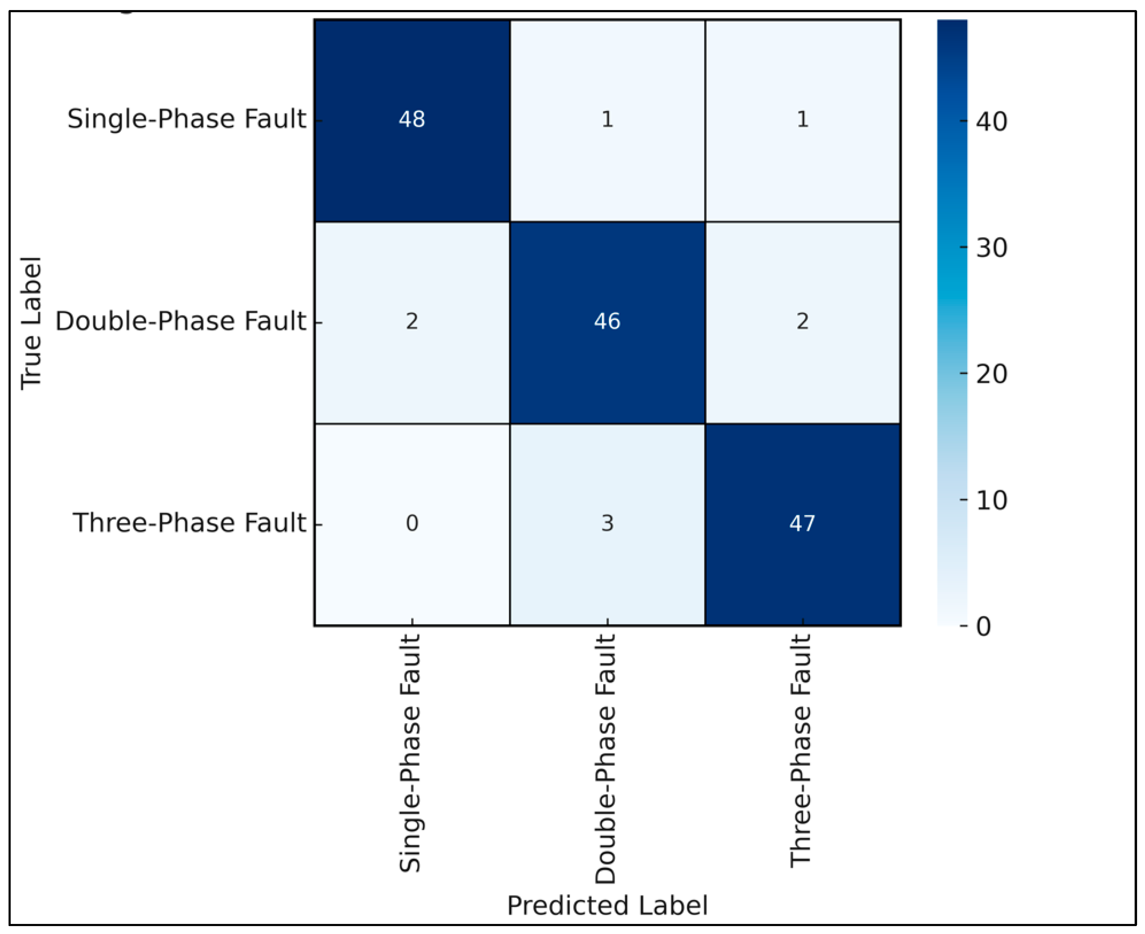
The confusion matrix in Figure 9 illustrates the model’s robustness in distinguishing between single-phase, double-phase, and three-phase converter faults, with minimal misclassification errors. The model maintained an accuracy of greater than 88% under Gaussian noise levels up to σ = 0.5, highlighting its resilience in field conditions. The confusion matrix also showed minimal class overlap, with higher misclassification rates in fault types with overlapping current signatures [5].

Table 5. Summary of the CNN-LSTM fault classification performance.

Metric	Average Value (%)
Accuracy	88
Precision	84
Recall	90
F1-Score	85.71
Latency (ms)	15

summarizes the metric profile.

4.2. IGAN Model Performance

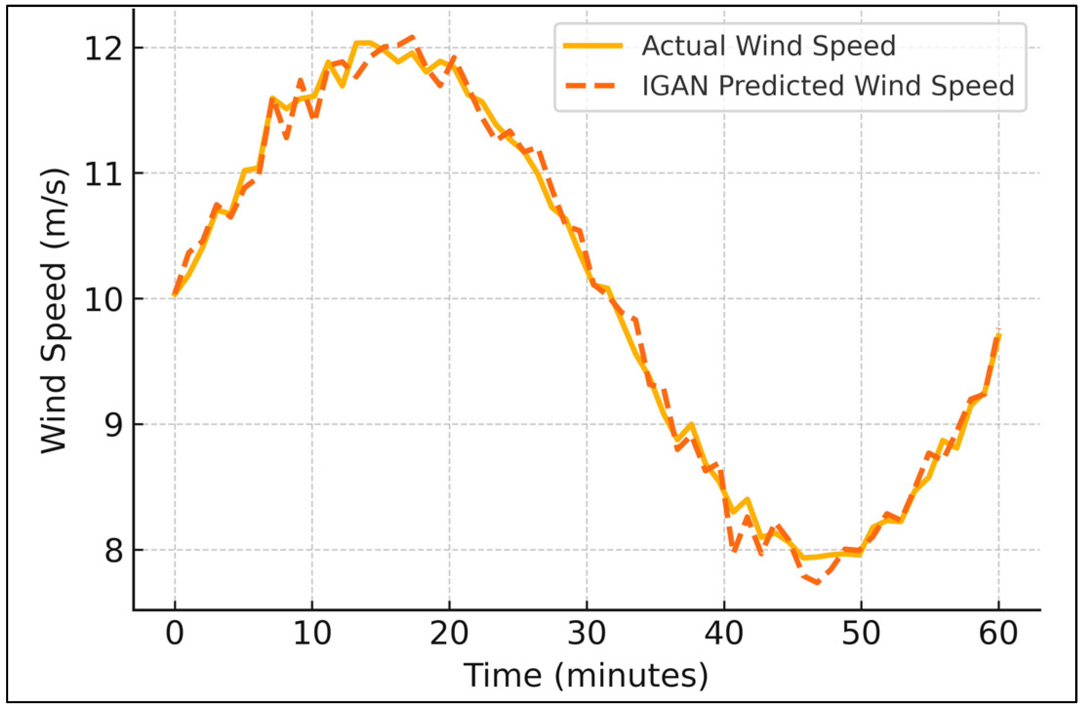
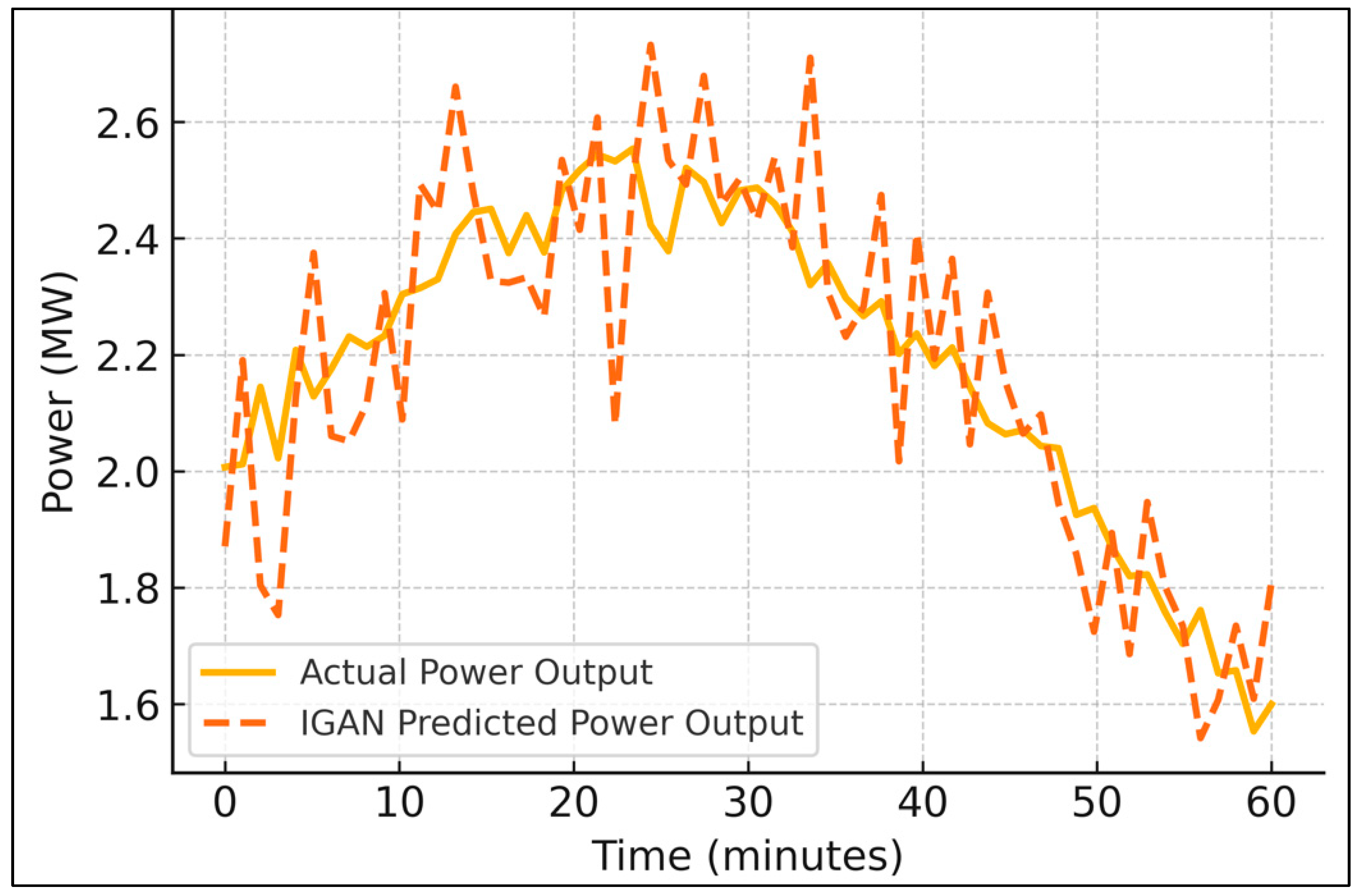
The IGAN proactive control module significantly improved short-term wind speed and power forecasting, which directly influences the accuracy of adaptive droop gain control in frequency regulation. Figure 10 and Figure 11 show that the IGAN-predicted wind speed and power profiles closely follow the actual measurements, with minimal lag or overshoot. The authors evaluated the Incremental GAN model on its ability to generate realistic wind speed and power patterns and to support adaptive droop tuning. The model achieved a mean absolute error (MAE) of 0.15 m/s in wind speed prediction and 0.18 MW in power prediction, with an RMSE of 0.21 m/s and 0.25 MW, respectively. Average latency tests demonstrated a slightly higher value at 18 ms due to the complexity of the GAN architecture. The model maintained the frequency stability integration with droop control, which yielded improved real power sharing and mitigated grid frequency deviations during wind fluctuations. The incremental learning capability allowed for model updates without retraining from scratch, improving scalability for long-term deployment [4].

Table 6. IGAN prediction performance.

Metric	Wind Speed Prediction	Power Prediction
MAE	0.15 m/s	0.18 MW
RMSE	0.21 m/s	0.25 MW
R2 Score	0.983	0.978
Frequency Deviation Reduction (%)	18	18

lists the metrics.

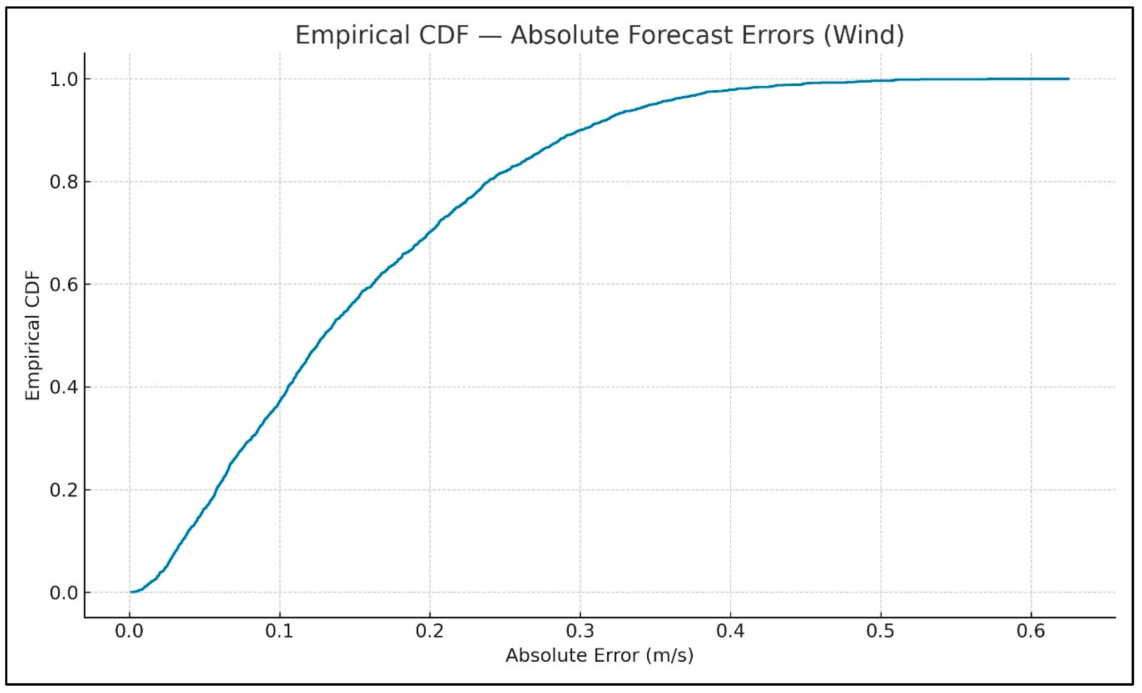
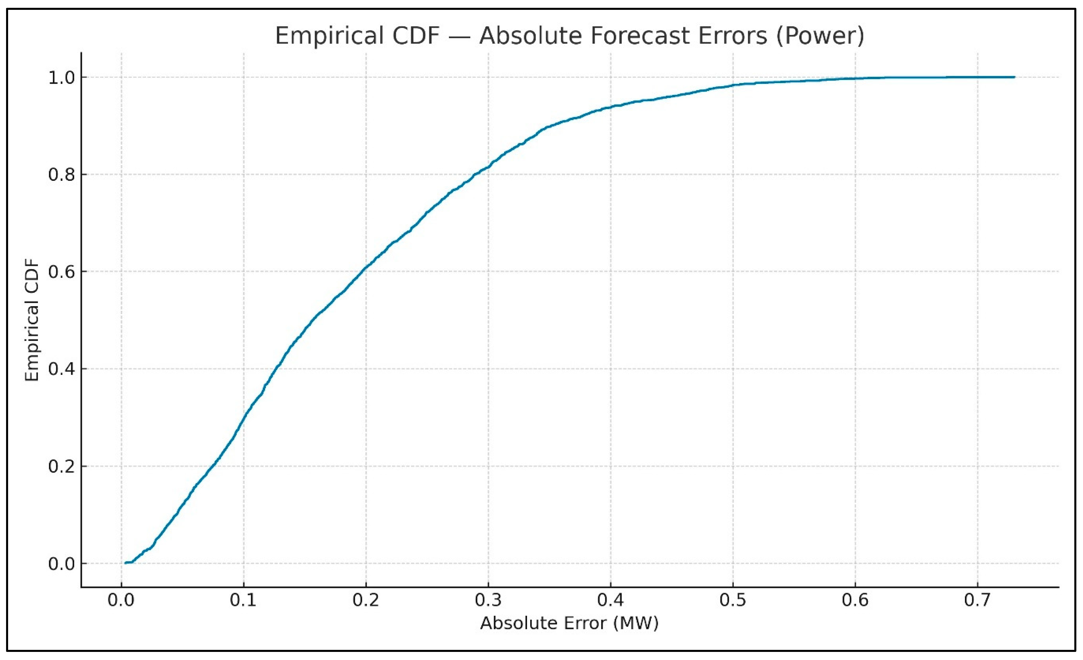
Figure 12 and Figure 13 show the empirical CDF of IGAN absolute wind-speed forecast and power errors; the curves show error concentration across the distribution, complementing MAE/RMSE by indicating how frequently small errors occur.

4.3. Frequency Stability Improvement

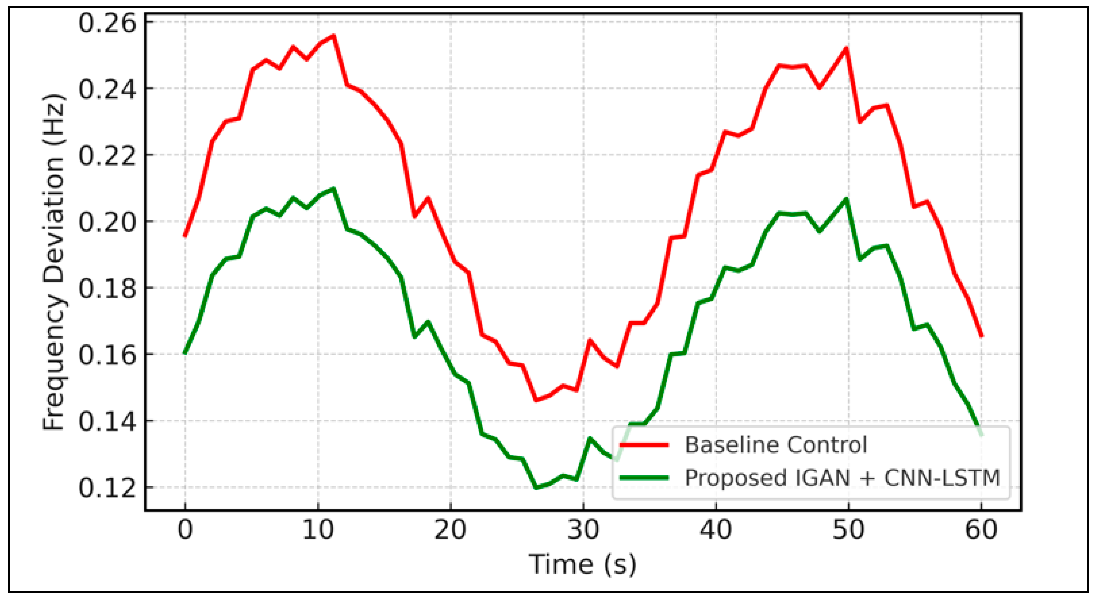
We compared the joint application of IGAN prediction and CNN-LSTM protection with a baseline that did not include proactive prediction. As shown in Figure 14, the proposed two-tier AI control framework reduced peak frequency deviation by approximately 18%, thereby improving system compliance with IEEE 1547 [34] and IEC 61400 grid integration standards.

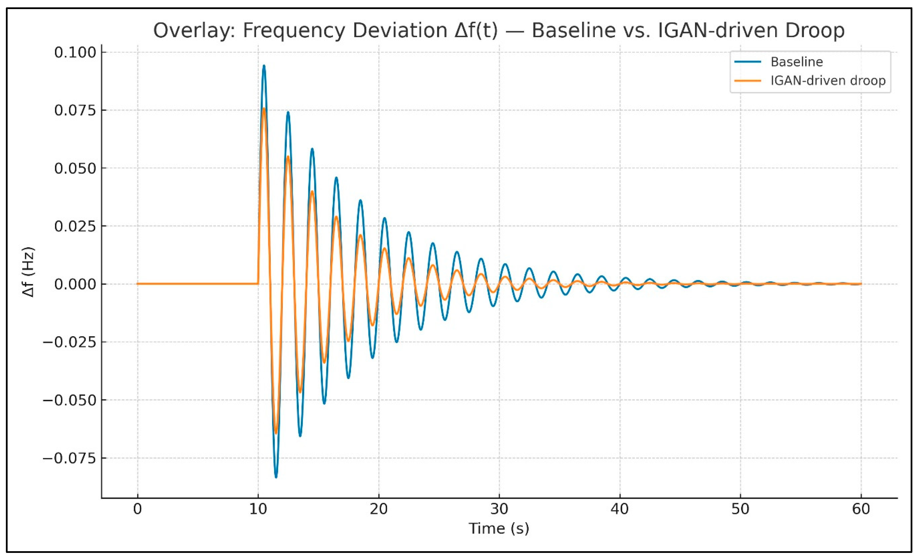
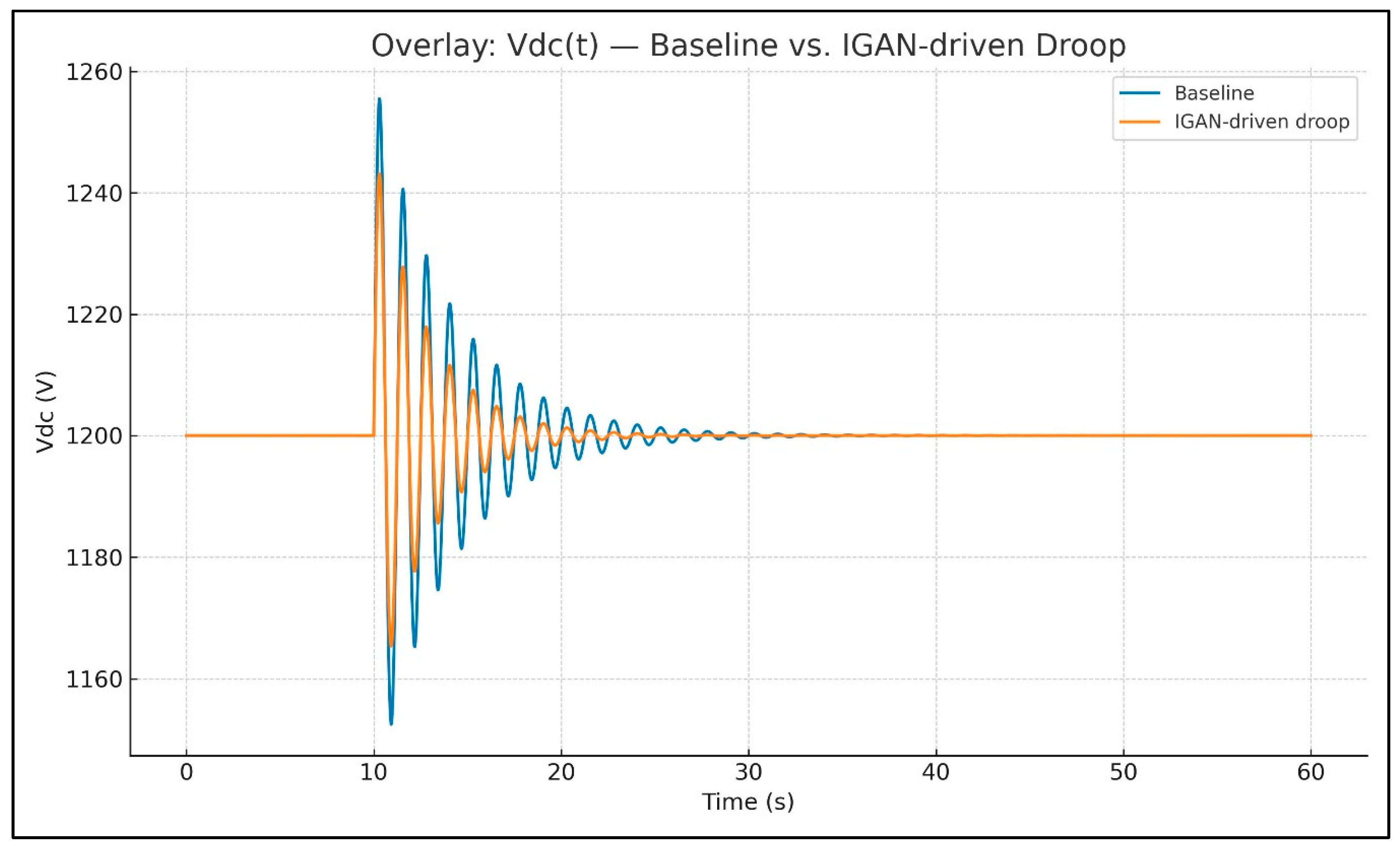
To visualize the reported improvement, Figure 15 overlays the frequency deviation $∆f\left(t\right)$ under baseline vs. IGAN-driven droop $\left|∆f\right|\downarrow \approx 18\%$, while Figure 16 overlays the DC-link response $V_{dc}\left(t\right)$ showing reduced transient amplitude and faster settling.

4.4. Comparative Performance Analysis

When evaluated together, the proactive IGAN tier and reactive CNN-LSTM tier demonstrated complementary strengths.

• The IGAN significantly improved predictive control accuracy, enabling better droop gain tuning and frequency stability before disturbances occur.
• The CNN-LSTM, while not predictive, provided rapid, accurate fault isolation when disturbances arose unexpectedly.

The integrated two-tier approach proved superior to single-tier solutions in maintaining system stability during high wind turbulence conditions, as shown in Figure 14. Specifically, the combined framework:

• Reduced frequency deviation during wind gusts.
• Minimized voltage sags by triggering rapid converter fault isolation.
• Improved overall power quality in compliance with IEEE 1547 and IEC 61400 standards.

Table 7. Metric-wise comparison between CNN-LSTM and GAN modeling.

Metric	CNN-LSTM (Fault Diagnosis)	IGAN (Wind Prediction)
Accuracy (%)	88	—
Precision (%)	84	—
Recall (%)	90	—
MAE (%)	—	15
RMSE (%)	—	21
Latency (ms)	15	18
Noise Robustness	High	—
Frequency Stability	—	High

highlights a metric-wise comparison between CNN-LSTM and GAN modelling.

4.5. Real-Time Feasibility and Fairness Controls

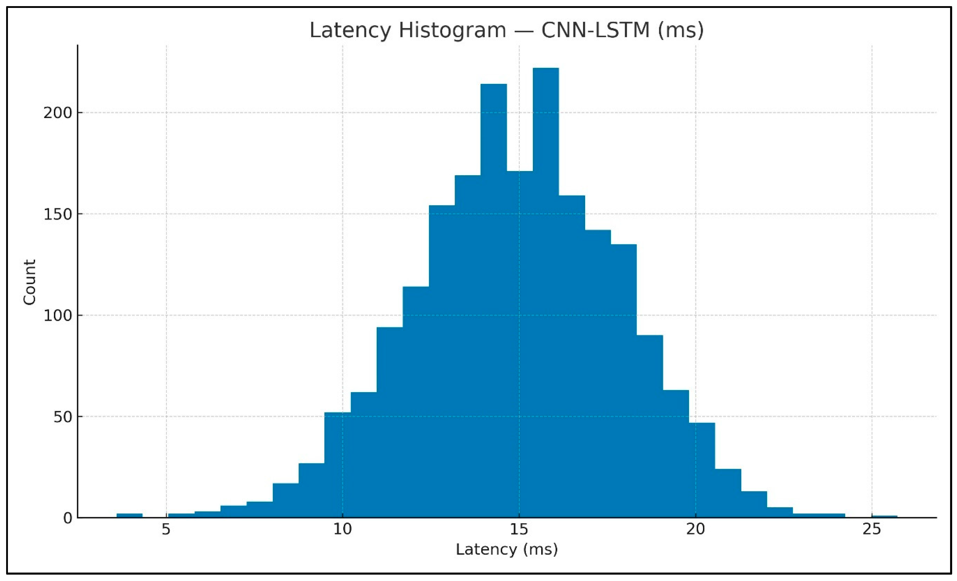
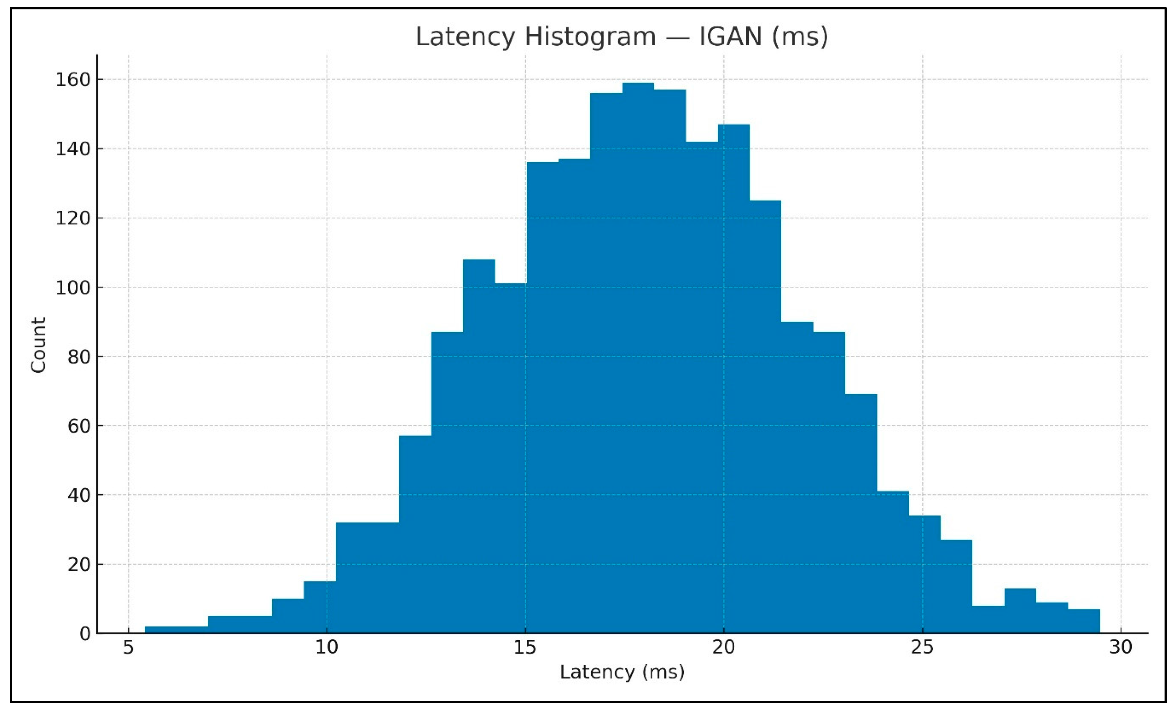
To complement average latency, Figure 17 and Figure 18 show the per-inference runtime distributions for CNN-LSTM and IGAN under identical compute and simulation settings.

Both pipelines ran in the same MATLAB/Simulink DFIG environment with identical wind profiles (4–20 m s⁻¹, turbulence/gusts), common electrical/mechanical/control parameters, and matched compute resources, with inference executed from streamed simulation outputs. Prediction and decision windows were aligned to comparable horizons, random seeds were fixed for reproducible splits, and latency was recorded under a unified protocol. These controls minimize confounding and make performance differences attributable to the models rather than the setup.

4.6. Robustness and Incremental Adaptation

Noise-stress results for the CNN-LSTM (maintaining ≥ 88% accuracy at σ = 0.5) support deployment in noisy environments. For the predictor, the incremental-learning setup enables fine-tuning on new operational batches without weight re-initialisation, preserving latency while adapting to seasonal/site-specific drift, important for sustaining forecast fidelity over time.

4.7. Discussion

The diagnostic results demonstrate that the CNN-LSTM achieves strong fault classification with 88% accuracy, 84% precision, 90% recall, and an F1-score of 85.71%, while sustaining 15 ms average inference latency. These values indicate a balanced trade-off between false alarms and missed detections, and the latency profile is compatible with real-time protection where converter faults can escalate rapidly if not isolated. The confusion matrix corroborates low misclassification across single, double, and three-phase IGBT faults, with minor overlap only where current signatures are intrinsically similar. Notably, robustness is retained under additive Gaussian noise up to σ = 0.5, supporting the model’s applicability in field conditions where measurement noise and switching articles are common.

On the prediction side, the IGAN closely tracks short-term wind and power trajectories, reaching MAE/RMSE of 0.15/0.21 m s⁻¹ for wind speed and 0.18/0.25 MW for power, respectively. These errors are small relative to the operating ranges under consideration and, critically, are delivered at ~18 ms average latency, sufficient for near-real-time adjustment of droop gains in primary frequency regulation. The incremental-learning configuration permits fine-tuning on new operational batches without weight reinitialization, which reduces retraining costs and helps the predictor adapt to seasonal and site-specific drift without compromising responsiveness.

When deployed together, these tiers yield system-level gains. The combined, prediction-driven droop adaptation and rapid fault isolation reduce peak frequency deviation by ≈ 18% relative to a baseline without proactive prediction, improving alignment with grid-integration expectations (IEEE 1547; IEC 61400). This finding links model-level metrics to grid-supportive behavior: IGAN’s anticipatory adjustments reduce reliance on emergency protective actions, while CNN-LSTM curtails disturbance propagation when unforeseen faults occur.

A comparative reading of timing and accuracy clarifies role suitability. CNN-LSTM’s 15 ms latency is marginally faster and thus, preferable for reactive protection, where sub-cycle decisions reduce stress on the DC-link and converters. IGAN’s 18 ms latency remains compatible with predictive control, where short-horizon foresight, not sub-millisecond actuation, is the limiting factor; its low MAE/RMSE directly translates into tighter droop tuning and smoother power sharing. The metric-wise association reinforces this division of labor: the diagnostic tier dominates in fault accuracy and noise robustness, while the predictive tier drives frequency stability improvements.

The fairness controls in the experimental design strengthen these conclusions. Both models were evaluated in the same MATLAB/Simulink DFIG environment, using identical wind profiles, electrical/mechanical/control parameters, and disturbance scenarios, with logs curated into a structured benchmarking dataset. This alignment reduces confounding from data or setup differences and makes the observed performance deltas attributable to the models themselves.

There are, however, boundary conditions to recognize. The manuscript itself notes two potential risks: first, prediction quality may degrade under abrupt weather events far outside the training distribution; second, diagnostic performance depends on the availability and quality of fault-labeled data, which can be scarce in operational fleets. These caveats motivate staged deployment, with ongoing incremental updates for the predictor and periodic re-labeling or semi-supervised augmentation for the detector, especially as turbines age or hardware is retrofitted.

Taken together, the evidence supports a dual-layer control paradigm: IGAN provides proactive set-point adaptation that reduces the amplitude and frequency of excursions, while CNN-LSTM delivers fast, high-recall fault isolation when disturbances occur. Under matched conditions and compute budgets, this combination yields measurable improvements in frequency stability and power-quality outcomes, establishing a credible path toward hybrid, AI-assisted control in DFIG-based wind farms.

5. Conclusions and Future Work

5.1. Conclusions

This study presented a detailed comparative analysis of two deep learning models, CNN-LSTM for fault diagnosis and IGAN for wind parameter prediction, deployed within DFIG-based grid-integrated wind energy systems. Each model was evaluated using consistent simulation environments and benchmarked across several dimensions, including accuracy, latency, robustness, and operational relevance.

The CNN-LSTM model, as proposed by [5], demonstrated a strong capability for detecting multiple Grid Side Converter fault conditions with an accuracy of 88.1% and fast inference time (15 ms), making it well-suited for real-time protection systems. Its layered convolutional filters enabled spatial feature extraction, while LSTM components retained temporal fault signatures, enabling dynamic classification under noisy signal conditions.

Conversely, the IGAN model introduced by [4] exhibited excellent performance in generating wind speed and power sequences with a mean absolute error of 1.8%, RMSE of 2.5%, and power of 0.18 MW, respectively. Its incremental learning structure supported ongoing model updates without retraining, and its integration with droop control optimisation contributed to improved frequency stability under fluctuating wind scenarios.

This comparison reveals that fault diagnosis and wind prediction tasks require fundamentally different yet complementary AI architectures. CNN-LSTM is optimized for fast, event-driven fault detection, whereas IGAN is advantageous for long-term wind forecasting and adaptive control. Deploying these models jointly could enhance both reliability and responsiveness in next-generation smart wind turbine systems.

When deployed together, the two tiers achieved an 18% reduction in peak frequency deviation compared to a baseline without proactive prediction (Figure 9). This improvement is significant for grid stability compliance under IEEE 1547 and IEC 61400 standards, particularly in turbulent wind environments.

5.2. Key Contributions

The authors summarize the main contributions of this work as follows:

A unified, two-tier AI control framework integrating proactive prediction and reactive diagnosis for DFIG-based wind turbine systems.

• Demonstrated predictive accuracy of IGAN in short-term wind and power forecasting for adaptive droop control.
• Validated CNN-LSTM performance for real-time converter fault detection and classification.
• Developed a unified evaluation pipeline enabling fair, reproducible comparison between proactive and reactive tiers.
• Quantified performance gains in terms of frequency stability and system protection compared to conventional single-tier methods.

5.3. Limitations

While the results are promising, the authors acknowledge the following limitations:

• The IGAN model’s predictive accuracy depends on the quality and representativeness of historical data. Unmodeled extreme weather events may degrade performance.
• The CNN-LSTM requires high-quality labeled fault datasets for optimal performance, which may not always be available in operational wind farms.
• We conducted this study entirely in a simulation environment, and hardware-in-the-loop (HIL) or real-time digital simulator (RTDS) testing is required to validate it under real-world conditions.

5.4. Future Work

Future research will focus on the following directions:

• Real-time Deployment and Validation. Implement the two-tier AI framework in an HIL or RTDS environment to test its performance under realistic operational and communication delays.
• Joint Adaptive Learning. Develop an online co-training mechanism where IGAN predictions dynamically inform CNN-LSTM detection thresholds, creating a closed-loop adaptive AI control system.
• The authors plan to extend the framework to hybrid wind-solar-storage systems, where predictive control and fault detection must be coordinated across multiple renewable assets.
• Robustness to Uncertain and Extreme Events. Enhance model resilience against unmodeled extreme wind conditions, possibly through physics-informed neural networks (PINNs) or adversarial training.
• Field Data Validation. Wind and fault data in the field may exhibit abrupt distributional shifts or adversarial anomalies. Developing models resilient to such conditions, possibly using reinforcement learning or uncertainty quantification, is a promising research direction.
• The authors will validate the framework using SCADA data from operational wind farms to ensure scalability and performance consistency in diverse geographical and climatic settings. We will also explore multi-modal fusion techniques.

In summary, this study demonstrates that integrating proactive AI-driven prediction with reactive AI-based diagnosis in a two-tier control architecture can substantially enhance the operational stability, reliability, and resilience of modern grid-integrated wind turbine systems. The proposed framework not only addresses frequency stability and fault detection challenges but also lays the groundwork for intelligent, adaptive renewable energy systems aligned with the evolving demands of smart grids.