Implications of Spatial Reliability Within the Wind Sector

Abstract

Distributed energy systems have gained increasing popularity due to their plethora of benefits. However, their evaluation in terms of reliability mostly concerns the time frequency domain, and, thus, merits associated with the spatial scale are often overlooked. A recent study highlighted the benefits of distributed production over centralized one by establishing a spatial reliability framework and stress-testing it for decentralized solar photovoltaic (PV) generation. This work extends and verifies this approach to wind energy systems while also highlighting additional challenges for implementation. These are due to the complexities of the non-linear nature of wind-to-power conversion, as well as to wind turbine siting, and turbine model and hub height selection issues, with the last ones strongly depending on local conditions. Leveraging probabilistic modeling techniques, such as Monte Carlo, this study quantifies the aggregated reliability of distributed wind power systems, facilitated through the capacity factor, using Greece as an example. The results underscore the influence of spatial complementarity and technical configuration on generation adequacy, offering a more robust basis for planning and optimizing future wind energy deployments, which is especially relevant in the context of increasing global deployment.

1. Introduction

Reliability comprises a fundamental problem measurement across all scientific disciplines. Originally stemming from the theory of probability and statistics, which was introduced by the likes of Blaise Pascal and Pierre de Fermat in the 1600s, in an attempt to answer gaming and gambling questions, and further expanded on by Pierre-Simon Laplace in the 1800s [1], its first recorded usage can be traced back to 1816 by English poet Samuel T. Coleridge [2]. Despite the aforementioned pioneers, reliability was only established as a scientific discipline in the early 1900s, owing to the rise of mass production for the manufacturing of large quantities of goods from standardized parts [3]. Its definition significantly varies from one discipline to another. For instance, in clinical studies, reliability refers to the consistency or repeatability of measurements [4]. In engineering systems, it is defined as the probability that a system will perform its required function, such as maintaining its structural integrity or adequately delivering its intended services, for a specified period of time under stated conditions [5,6].

Acknowledging the ever-increasing global power demand, it is imperative to explore the concept of reliability within the energy sector, where consistent performance is not just desirable but also essential for economic stability and public safety. The reliability approach has been widely accepted as a benchmark for power system design and operation at all phases [7]. Overall, power system reliability is defined as the ability of an electric power system to accommodate an adequate supply of electrical energy under given conditions for a specified time interval [8]. In order to distinguish the focus of reliability indicators used in the literature, three hierarchical levels have been established: Hierarchical level I (HLI), which entails power generation, Hierarchical level II (HLII), which also considers transmission, and Hierarchical level III (HLIII), which accounts for the aforementioned while also assessing distribution [9].

The large-scale utilization of renewable energy sources (i.e., solar radiation, wind speed) for power generation has made HLI reliability indicators all the more relevant. Power systems with a high share of renewables face additional challenges with respect to reliability management. This is attributed to the intermittent nature of the primary drivers, since generation, availability and sufficiency exclusively depend on meteorological processes. Therefore, the reliability assessment of standalone renewable systems is rather austere, given that the slightest deviation from the satisfactory state (i.e., generation not exceeding the load demand for a given time step) is indicated as a failure, often yielding very low reliability scores. On the contrary, the reliability of renewable-based systems is very responsive to the addition of elements that allow for regulation and control, such as conventional generating units and storage components, which are predominantly used to achieve a desired level of adequacy.

The introduction of distributed generation (DG) by renewables, both grid-tied and standalone, has had a vital impact on the reliability of power systems. It has been proven that the proper injection of DG into power systems can ameliorate both generation and distribution reliability [10,11]. From the generation perspective, DG systems leverage the geographical smoothing phenomenon, arising from the spatial scale across which climatic conditions vary, leading to a smoother and less intermittent power output by renewable sources [12]. This aspect is especially crucial for wind power generation [13,14], which is not only dependent on the spatiotemporal variability in wind speed [15,16] and local topography [17], but also on the non-linear dynamics introduced by the wind power curves [18].

The increasing uncertainties associated with renewable energy systems introduce additional complexity into the estimation of reliability. To address this, probabilistic indicators are preferred over deterministic ones to assess system performance, as they capture uncertainty in a more appropriate manner, accounting for both the severity and probability of events [8]. However, the challenge of quantifying the reliability of distributed energy resources persists as their penetration increases.

A recent study introduced the concept of spatial reliability of distributed energy resources, establishing a framework for estimating their combined generation capacity over a specified region in probabilistic means, and applied it to solar photovoltaic (PV) energy over the region of Greece [12]. More specifically, the power output was estimated and was expressed through the mean annual capacity factor by randomly distributing PVs across 40 representative locations in a Monte Carlo setting. This approach draws inspiration from the spatial complementarity of renewables; the scarcity of one source in site x is complemented by its availability in site y at the same time, t [19].

Building on the rationale of Zisos et al. [12], the objective of this work is to validate this framework in the context of wind power and to quantify the implications of its inherent uncertainties on generation output. In contrast to solar energy, the application of this framework to wind power is more complex, owing to a range of additional considerations regarding siting and wind turbine model selection, as outlined below.

First, several wind turbine placement criteria concerning the macro- and micro-scale dictate the suitable candidate sites, inhibiting the arbitrary selection of installation locations. Additionally, the non-linear relationship between a turbine’s power output and its primary and derived parameters is governed by the power curve, a turbine-specific feature that significantly varies from one model to another.

Notably, the actual potential of a given location can be accurately represented only if turbine selection accounts for both the available wind power and for the wind speed distribution [20]. Hence, assessing a location’s potential merely based on the derived power output of an arbitrary selected turbine may result in misleading conclusions about its true generation capacity.

Another parameter that requires thorough investigation prior to turbine selection is the hub height, which also features a major role in generation output. Since wind speed increases with height, commonly modeled by a power or logarithmic law in the literature, even the smallest increases in hub height can lead to significant differences in power output [21]. In this context, it is important to remark that the highest turbine does not necessarily have to be the most energetically productive in every kind of localization [20].

This article is organized as follows. Section 2 provides a brief overview of the spatial reliability rationale and its quantification techniques and outlines the additional necessary actions to adapt and apply this framework to the wind sector. Section 3 initially provides the study area and the data sources utilized, followed by the background analysis to calculate wind power output, and, therefore, estimate the generation potential of various centralized configurations (hereafter referred to as the “baseline” scenario). The latter are then contrasted with spatially dispersed configurations (facilitated through a Monte Carlo Simulation) and respective scale–yield–reliability laws are derived. The derived scaling laws are contrasted with the ones concerning the framework’s application to solar PV energy. Section 4 provides a discussion of additional considerations pertinent to the broader context of this analysis and highlights future research directions. Finally, Section 5 summarizes the key findings of this work.

2. The Rationale Behind Spatial Reliability

2.1. Theoretical Background

The previous section provided an overview of reliability, with a particular focus on renewable-based systems in distributed generation settings. Undoubtedly, DG offers a range of benefits, such as enhanced efficiency and greater flexibility in load management, compared to that of centralized configurations [22,23]. However, common reliability indicators found in the literature mainly focus on the temporal scale (for this reason, it is also referred to as time-based or occurrence-based reliability), and thus fail to capture the spatial dimension and its associated merits (i.e., spatial complementarity and geographical smoothing). In an attempt to address this gap, Zisos et al. recently introduced the novel concept of spatial reliability for renewable energy systems, defining it as the probability of achieving a guaranteed level of power production over a given region [12]. The generic mathematical expression, following the inverse problem formulation of reliability (i.e., a constant yield or yield pattern that can be achieved for a specific reliability level) [24] is posed as follows:

$$a≔1-\mathrm{𝒫}\left[Y\left(s\right)<D\left(s\right);s\in \Omega \right]$$

(1)

where $\mathsf{\Omega }$ denotes a certain spatial domain, and $Y\left(s\right)$ and $D\left(s\right)$ refer to the energy yield and associated demand at a certain site, respectively. Since Equation (1) does not have an analytical solution, unless the yield, $Y\left(s\right)$, follows a simple probabilistic structure and the demand, $D\left(s\right)$, is constant, Monte Carlo approaches are considered most appropriate. They typically entail the representation of the randomly varying processes $Y\left(s\right)$ and $D\left(s\right)$ through a simulation model that accounts for the probabilistic/stochastic regime of failure events and their associated frequencies of occurrence [24].

Similarly to how temporal reliability is handled, the space domain $\Omega$, although continuous, is typically discretized in order to reduce model complexity and computational burden. This is achieved by dividing $\Omega$ into sub-areas (e.g., by delineating a mesh grid) and assigning a single value to each sub-area, i.e., a spatial average, regarding energy yield. Notably, one can even estimate spatial reliability solely based on a set of individual points, provided that these points adequately capture the entire area’s spatial variability in power production.

A key aspect of estimating spatial reliability is expressing the energy yield $Y\left(s\right)$ in a form that is independent of case-specific conditions (e.g., installed capacity), thereby enabling comparisons across different systems, locations and configurations. A commonly used metric for this purpose is the capacity factor (CF), which assesses the performance of energy systems, providing an estimate of the generation potential over a specific period of interest. It is defined as the ratio of actual electricity production, $E$, to the theoretical maximum output that could be generated by a system (or a collection of systems) with a total power capacity $P_{max}$ over the time interval, $T$:

$$CF={\displaystyle \frac{E}{P_{max} T}}={\displaystyle \frac{{\int }_0^{T}P\left(t\right)dt}{P_{max} T}}$$

(2)

On an annual basis, which is the typical time interval considered in energy assessment studies, the mean annual capacity factor of a power system contrasts with the mean annual energy yield with its theoretical maximum, assuming its continuous operation at full capacity, i.e., for $T$ = 8760 h. In order to capture the overall performance of common renewable energy systems, which is mainly dictated by the statistical regime of the driving climatic processes (solar, wind, hydro), the time interval $T$ should span over a much more extended period, thus reflecting the full spectrum of climatic variability and being little influenced by low-frequency events and local extremes. As such, the yield function $Y\left(s\right)$ in the context of spatial reliability studies is recommended to be expressed in terms of the mean annual capacity factor.

2.2. Adaptation to Wind Power

The concept of spatial reliability has previously been applied and validated in decentralized solar PV configurations [12]. However, extending this concept to the wind sector is a considerably more complex exercise as it involves both siting constraints and numerous factors that influence the transformation of wind speed into power output.

The first aspect concerns turbine siting. The optimal selection of a wind turbine site (or, more generally, a system of turbines comprising an Aeolic park), is a multidimensional problem, which entails factors such as wind resource adequacy, land availability, environmental conditions, the possibility of connection to the electrical transmission system and the design of auxiliary facilities [25,26]. A common siting practice has been to iteratively place the wind turbines in positions that exhibit the greatest potential whilst ensuring adequate distance between them in the prevailing wind direction to prevent any excessive wake effects [27]. In the present study, the wind turbine siting procedure is performed only taking into account the wind resource potential and its primary determinant factors (i.e., wind speed distribution, effects of topography). This approach expands the set of available installation locations, which is desirable in order to investigate wind power potential in a fully distributed and theoretical setting. The locations are selected through the Global Wind Atlas (GWA), a validated high-resolution database that contains long-term data about wind processes (e.g., speed, distribution, direction), accounting for topographic effects, which is widely used in wind power feasibility studies [28].

The second element concerns the wind-to-power transformation, typically employed through the power curve, which is primarily used in the estimation of wind energy potential, turbine selection and condition monitoring, and wind power forecasting [18]. At a given time, if the wind speed at the turbine hub height falls within the range of the cut-in speed ($V_{cut-in}$) and the rated speed ($V_{rated}$), the power conversion is dictated by a non-linear relationship. In the literature, this relationship is commonly modeled either by deterministic means, often using high-order polynomial equations [29,30], multi-parametric models [31,32] or artificial-intelligence-based approaches (e.g., neural networks, fuzzy clustering, copulas) [33,34,35], or by probabilistic methods (e.g., Gaussian Process, full probability regression models) [36,37]. Unlike previous methods, this study considers an analytical formula, utilizing only the cut-in and rated wind speeds, as well as the nominal power, $P_{nom}$, of the selected turbine as follows:

$$P_{wind}=\left(1-{\left(1-{\left({\displaystyle \frac{V_{\mathit{wind}}-V_{\mathit{cut}-\mathit{in}}}{V_{\mathit{rated}}-V_{\mathit{cut}-\mathit{in}}}}\right)}^a\right)}^b\right)P_{\mathit{nom}}$$

(3)

where $a$ and $b$ are shape parameters, calibrated against the actual manufacturer power curve. The use of two shape parameters offers significant flexibility, at the same time being much more parsimonious than the most widely used approach of polynomial expressions. Furthermore, it explicitly accounts for the actual technical characteristics of the turbine considered, i.e., $P_{nom}, V_{cut-in}$, and $V_{rated}$. 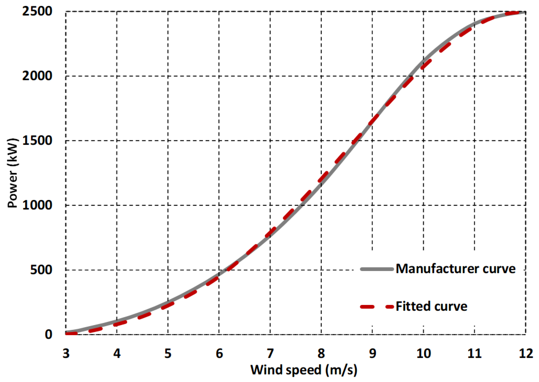An indicative non-linear region of a power curve against the fitted one is presented in Figure 1.

Lastly, one significant challenge that arises in accurately estimating the generation potential of each site is the selection of an appropriate turbine model. As already outlined in the introduction, this is a multicriteria decision-making problem that is subject to several factors, with the most sensitive one being the hub height. To avoid complex optimization techniques that are beyond the scope of this analysis, the authors test a sufficiently large sample of wind turbine models, with different characteristics, in each considered location, iteratively calculating their generation potential in means of the capacity factor. The average capacity factor of each site is then applied to approximate the locations’ true generation capacity. The rationale behind this key assumption is that the concept of spatial reliability refers to power systems that are dispersed across large regions (e.g., on the national scale). In this vein, their development is asynchronous, thus comprising individual elements (in the case of Aeolic energy, wind turbines) of heterogenous technologies and, potentially, design philosophies.

3. A Novel View of Greece’s Wind Potential Within the Spatial Reliability Framework

3.1. Study Area and Data Processing

This section implements the concept of spatial reliability in wind energy over Greece that goes far beyond previous studies that assess its wind potential in order to produce useful maps for site-specific planning and design studies [38,39,40].

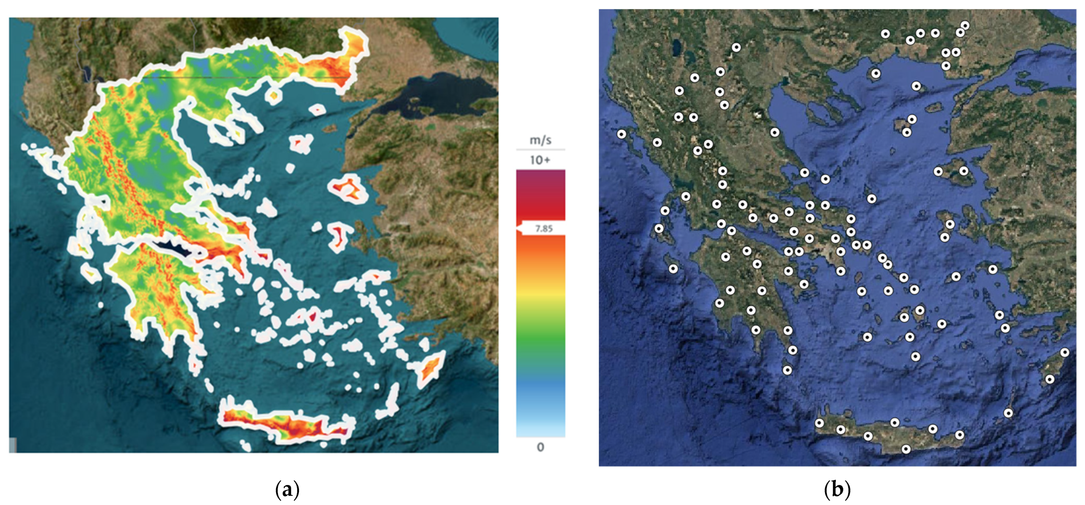
As shown in Figure 2a, Greece is characterized by high wind power potential, especially in the eastern coastal regions and the islands of the Aegean Sea [38]. More specifically, 100 spatially dispersed locations are selected (Figure 2b) based on their Aeolic potential, provided by the Global Wind Atlas, in terms of average wind speed at 100 m above ground level [41].

The $u$ (i.e., wind’s speed along the east–west zonal axis) and $v$ (i.e., wind’s speed along the north–south meridional axis) components of 10 m hourly wind speed time series for 20 years (2005–2024) across the 100 locations are retrieved from the Copernicus Climate Change Service (C3S) Climate Data Store (CDS) [42]. Specifically, the ERA5-Land reanalysis dataset [43] is utilized, with a spatial resolution of 0.10° (~9 km at the latitudes and longitudes considered here), which is finer than the one of ERA5 (0.25° which translates to ~25 km here). This finer spatial resolution allows for capturing local conditions in a more appropriate manner, considering that the coarser ERA5 dataset resolution was found to mask finer terrain effects on the wind field over regions with complex topography [44], despite it still having been proven reliable for wind power modeling [45,46,47]. Even though in situ wind speed data are not commonly available for the Greek region, to allow for validating the ERA5 dataset, the latter are in fact calibrated against a sufficient number of ground stations [43]; thus, the existing bias is expected to be low.

The total wind speed for each location is calculated as follows:

$$V_{wind}=\sqrt{v^2+u^2}$$

(4)

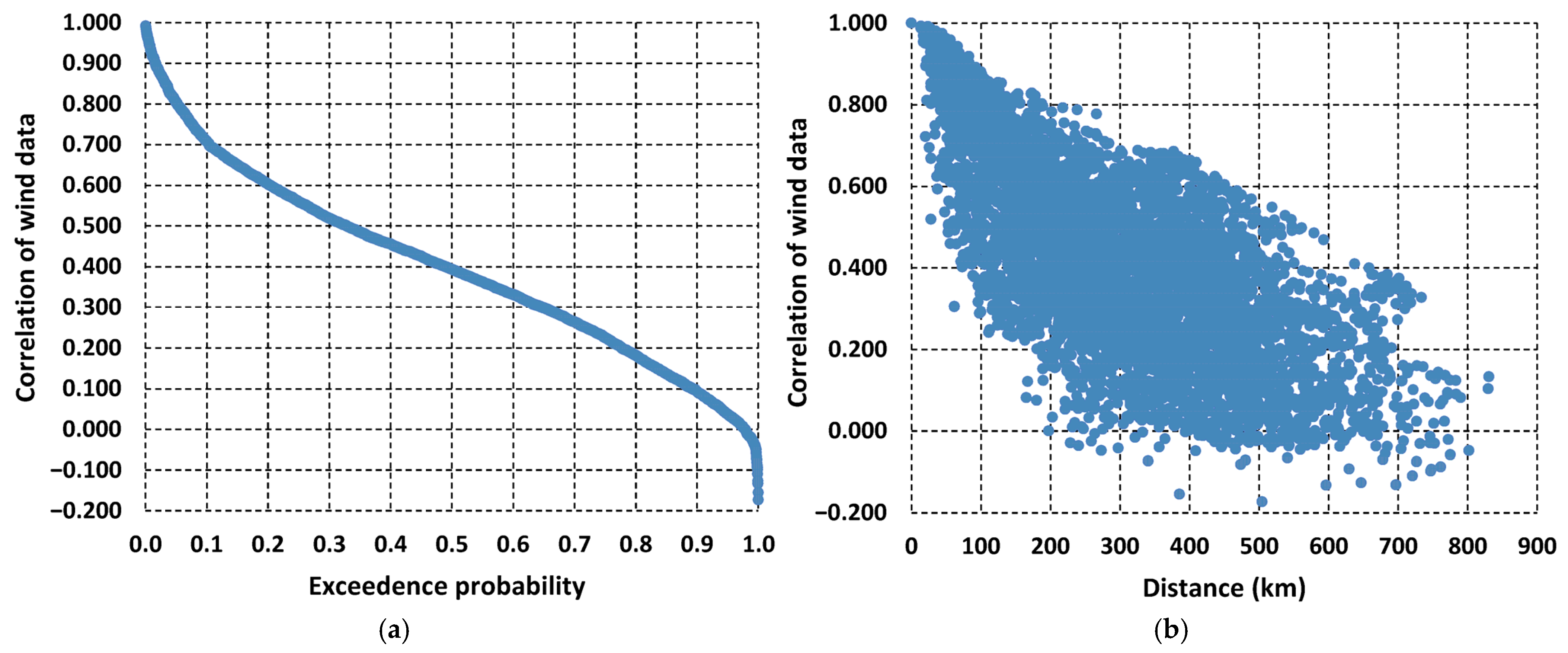
Before proceeding to wind power generation simulations, each location is verified against its mean annual speed, ensuring values exceeding 4.0 m/s, which is the legal national threshold for wind projects. Furthermore, a spatial dependence analysis is employed by calculating Pearson’s correlation coefficients of hourly wind data among all pairs of locations (thus yielding 4950 values). The key outcomes of this analysis are demonstrated by the two key diagrams of Figure 3, both indicating that the selected locations are well distributed. As shown in Figure 3a, the correlations are generally moderate to low (and even negative), while only 2% of pairs exhibit significant correlations, of the order of 90%. As expected, the correlations decrease with distance (Figure 3b), yet their spread is quite significant even for relatively small distances (i.e., up to 50 km), since the wind regime over Greece is also influenced by the exceptionally fragmented relief characteristics (particularly, orography).

3.2. Background Analysis

As explained in Section 2.2, in order to capture each location’s actual generation potential, 40 turbine models with different technical characteristics and hub heights, ranging from 58 to 136 m, are applied at each site and a total of 85 capacity factors are estimated for each location based on Equation (2). This is achieved by fitting Equation (3) to each turbine’s power curve to determine the shape parameters that will be used to calculate the hourly power output, and, subsequently, the capacity factors. It is emphasized that for each commercial turbine, the applicable hub heights (ranging from two up to five, depending on the model characteristics) are already specified by the manufacturers.

Prior to estimating the wind power output, the wind speed time series of all locations are adjusted to the associated hub heights, according to the following logarithmic law:

$$V_2=V_1\left({\displaystyle \frac{\mathit{ln}\left(\frac{z_2}{z_0}\right)}{\mathit{ln}\left(\frac{z_1}{z_0}\right)}}\right)$$

(5)

where $V_1$ is the given wind speed, estimated through Equation (4), $z_1$ is the distance from the ground (i.e., 10 m), $z_2$ is the wind turbine hub height, and $z_0$ is the surface roughness parameter. The last is considered equal to 3 cm, a value that corresponds to typical onshore wind turbines on rural open areas with flat terrain, sparse vegetation or plough land [48,49]. It is highlighted that surface roughness is an inherently uncertain parameter, which is influenced by complex factors such as vegetation height and density, canopy structure, terrain properties, buildings, etc. Furthermore, it is also subject to epistemic uncertainties originating from the turbulence theory within Equation (5), since, in fact, $z_0$ is an empirical parameter without rigorous physical interpretation [50]. Nevertheless, the effect of surface roughness diminishes with height, $z_2$, thus making the conversion procedure not very sensitive against this parameter. 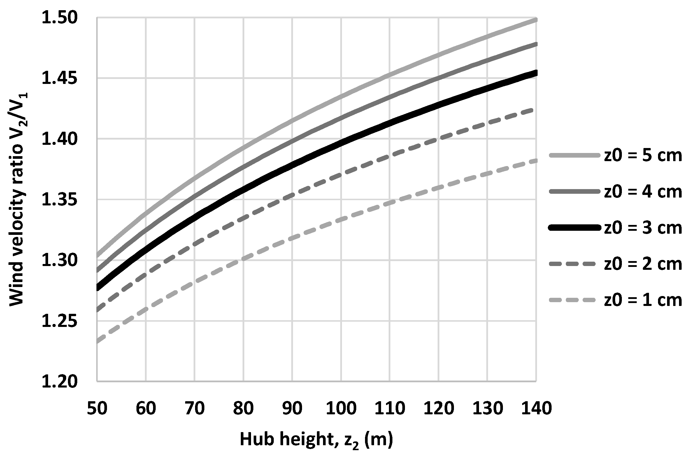This is also evaluated through a sensitivity analysis, employed for the range of hub heights applied in this study, where the conversion ratio $V_2/V_1$ for the applied value of $z_0$= 3.0 cm, as function of $z_2$, is contrasted with four other surface roughness values, i.e., 1.0, 2.0, 4.0 and 5.0 cm, that can be found in wind farms (the two extremes are applicable for rough pasture terrains and crops, respectively). As shown in Figure 4, the differences with respect to ratio $V_2/V_1$ are of the order of 1–5%, thus confirming the relatively low sensitivity of parameter $z_0$. It is remarkable that the impacts in terms of output electricity production and, eventually, capacity factor will be even less important, given that for a wide range of wind speeds, the turbines operate at their nominal capacity.

The hourly wind power production is estimated based on each turbine model’s power curve. In this vein, the analytical formula introduced in Equation (3) is used, which ensures a very good approximation of the power curves provided by the turbine manufacturers. More specifically, based on the wind speed at a given time, the power output is derived as follows:

$$P_{hourly}=\left\{\begin{array}{c}0, V_{wind}<V_{cut-in}\\ \mathit{Equation} \left(2\right), V_{cut-in}\le V_{wind}<V_{rated}\\ P_{nom}, V_{rated}\le V_{wind}<V_{cut-out}\\ 0, V_{wind}\ge V_{cut-out}\end{array}\right.$$

(6)

where $V_{cut-out}$ is the wind speed at which the turbines are designed to automatically shut down or reduce power output to prevent damage, herein assumed to be 25 m/s, and the shape parameters of Equation (2) (i.e., $a$, $b$) are inferred via calibration to each of the selected power curves.

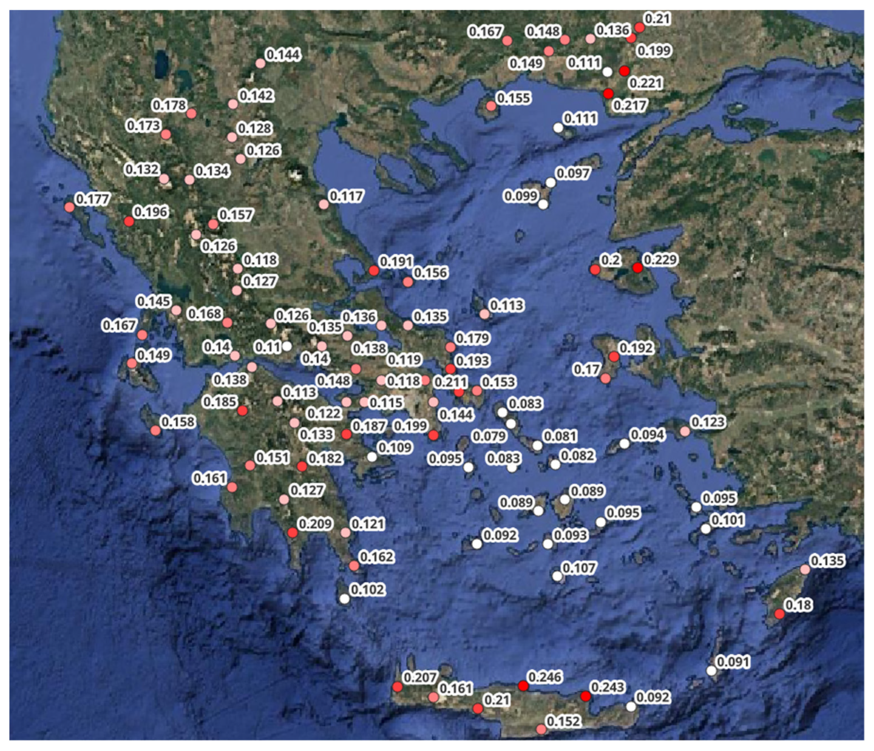
Furthermore, the mean value of the 85 capacity factors is calculated (Figure 5), which reflects each location’s average generation potential. The derived values confirm the high Aeolic potential observed in the eastern coastal and islandic regions of the Aegean Sea. Additionally, Figure 6 demonstrates the capacity factors’ coefficients of variation (CV) for each location, which is a normalized measure of dispersion. Notably, locations that exhibit the highest wind potential (i.e., high mean CF values) have relatively low CV values, thus being not very sensitive against the specific turbine characteristics (by means of a commercial model, and thus power curve and hub height). On the contrary, high CV values are observed in locations where estimated CF values are lower, indicating the key role of turbine selection and sizing to ensure good performance.

The derived mean capacity factors of all locations are also contrasted with the corresponding values of GWA (Figure 7). The latter are derived from the convolution of a site’s long-term wind speed distribution at 100 m above ground level, with a representative power curve for each of the three International Electrotechnical Commission (IEC) classes of wind turbines [51]. To the purpose of this comparison, the class-I capacity factor is considered, which refers to the typical and most robust turbines. The so-called representative turbine has a nominal capacity of 3450 kW and a cut-off wind speed of 25 m/s.

Remarkably, the two variables exhibit a satisfactory coefficient of determination (R²), which is a macroscopic confirmation of data accuracy (i.e., wind speed, turbine model characteristics) and overall methodological soundness. Nevertheless, discrepancies between the two approaches are anticipated, considering that the GWA only accounts for one representative power curve, while this analysis is much more comprehensive, since it investigates a wide range of alternative turbine models and hub heights.

3.3. Baseline Scenario (Centralized Generation)

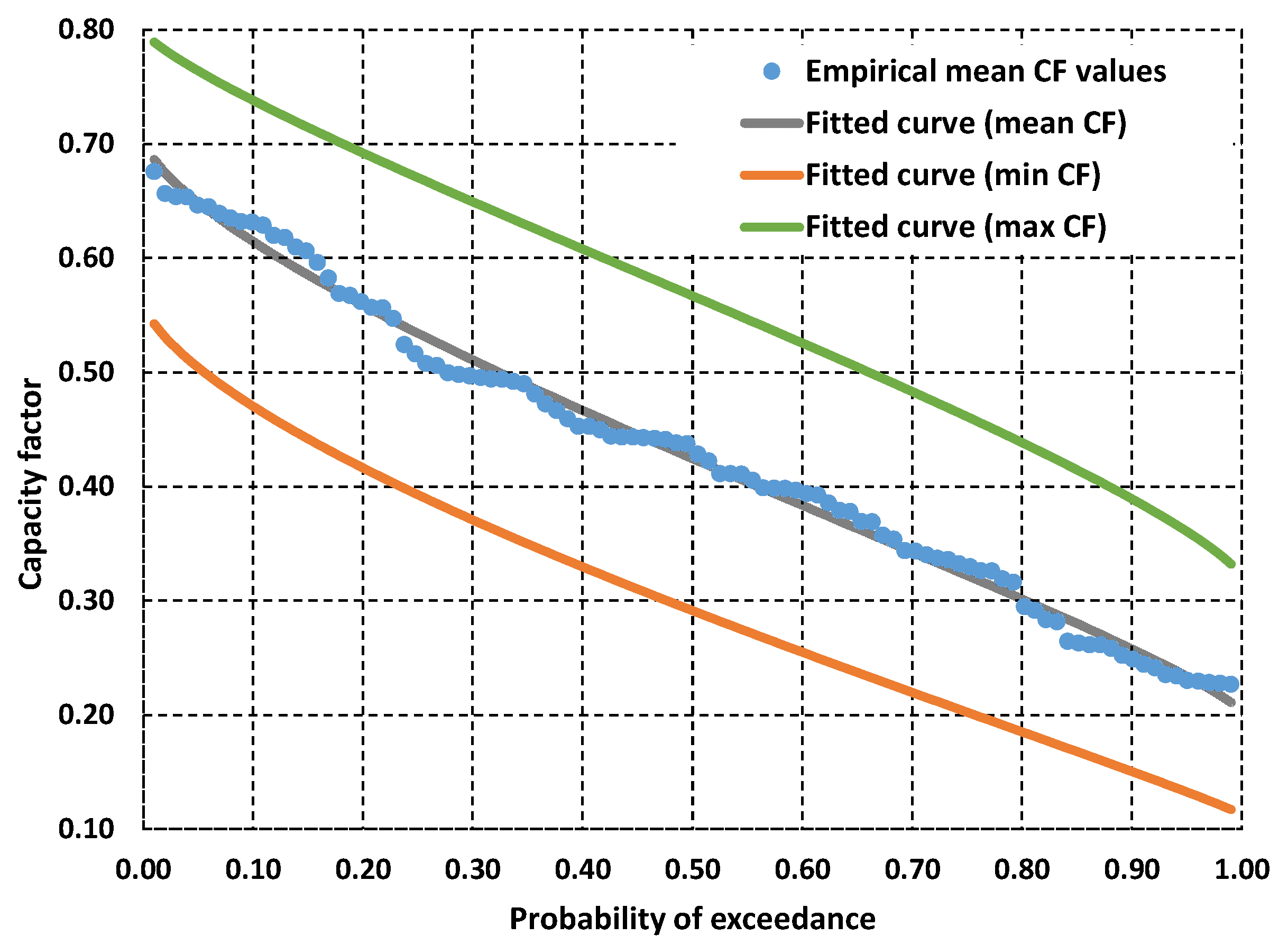
This section aims to investigate the potential of each location’s centralized generation by estimating their individual power production, a system layout which corresponds to the “baseline” scenario. The generation output variability across the selected locations is probabilistically expressed and visualized through the empirical probability curve (inverse cumulative distribution function) of the annual capacity factors, as formalized in Section 3.2. The output is a curve (Figure 8) that represents wind power potential (in the y-axis) with an exceedance probability assigned to each capacity factor value (in the x-axis). The probability of exceedance, in the context of this research, is interpreted as a spatial reliability metric. It reflects the percentage of locations that can guarantee a desired power output on an annual basis, and is calculated by sorting the capacity factor values in descending order and utilizing the Weibull formula, i.e., the following formula:

$${\mathrm{𝒫}}_{\mathcal{i}}={\displaystyle \frac{\mathcal{i}}{n+1}}$$

(7)

where $n$ is the number of locations considered and $\mathcal{i}$ is the sorting value position. The Kumaraswamy distribution is then fit to the $n$ capacity factor values to provide a continuous spatial probability model. This function is selected due to its double (lower and upper)-bounded nature, making it suitable for random processes that are known to have theoretical finite limits [52]:

$$CF=C{F}_{max}+[1-{\left(1-{\mathrm{𝒫}}^a\right)}^b](C{F}_{min}-C{F}_{max})$$

(8)

where $C{F}_{min}$ and $C{F}_{max}$ are the theoretical lower and upper limits of the capacity factor, respectively, $a$ and $b$ are shape parameters, and $\mathrm{𝒫}$ is the probability of exceedance. The shape parameters and the limits of $C{F}_{min}$ and $C{F}_{max}$, corresponding to values of $\mathrm{𝒫}\approx 1$ and $\mathrm{𝒫}\approx 0$, respectively, are inferred via calibration.

As expected, although the theoretical limits of the capacity factor metric are 0 and 1, the derived upper and lower limit values for wind power across all examined locations (i.e., 0.70 and 0.20) are narrower while still exhibiting significant difference. This is attributed both to the spatial variability in wind speed across the examined locations and the wide spectrum of applied turbine technologies and hub heights. The last aspect is also demonstrated in the graph by plotting the associated probabilistic curves (in particular, the theoretical ones by fitting the Kumaraswamy distribution function to the data) for the minimum and maximum capacity factors. At each location, their dispersion ranges from 20 to 30%, thus indicating the strong uncertainty behind all existing wind potential mapping exercises, whose outputs are presumably rather sensitive to turbine model and hub height selection. Furthermore, it also confirms the authors’ key assumption regarding the use of the mean $CF$ as the basis for evaluating the spatial reliability concept.

Importantly, Figure 8 also verifies that the selected locations are favorable in terms of wind power generation. It can be observed that a capacity factor of 0.40, which is indicative of well-performing onshore wind farms in Greece, corresponds to a spatial reliability level of approximately 60%. This means that 60 out of 100 of the selected sites are guaranteed to achieve at least as much power as that implied by a capacity factor of 0.40.

3.4. Spatial Reliability Assessment

Quantifying the reliability, both temporal and spatial, of wind farms requires inputs that are driven by randomly varying processes (i.e., wind speed and direction), which are, therefore, inherently defined as stochastic. As already outlined in Section 2.1, an analytical derivation of spatial reliability is impossible since it is subject to the non-linear dynamics introduced within the wind-to-power conversion. In this vein, a Monte Carlo Simulation (MCS) is considered most appropriate, as it entails numerical procedures that accurately represent real-world systems in probabilistic means.

More specifically, the MCS is performed across 100 locations over Greece to assess wind power output in a distributed (decentralized) setting. The aim is to calculate the “joint” wind power potential (in terms of mean capacity factor) of spatially dispersed sites by distributing turbines in equally probable combinations of locations. Each combination stems from sampling the available number of locations within the range $[2, n-1]$, where $n$ is the total number of pre-specified locations (100, in this analysis). To ensure a satisfactory number of combinations is achieved while also handling combinatorial explosion and sustaining computational load within a feasible margin, 100,000 simulations are performed for each setting. The exceedance probability curves are then produced for all locations by fitting the Kumaraswamy distribution function to the empirically derived data. 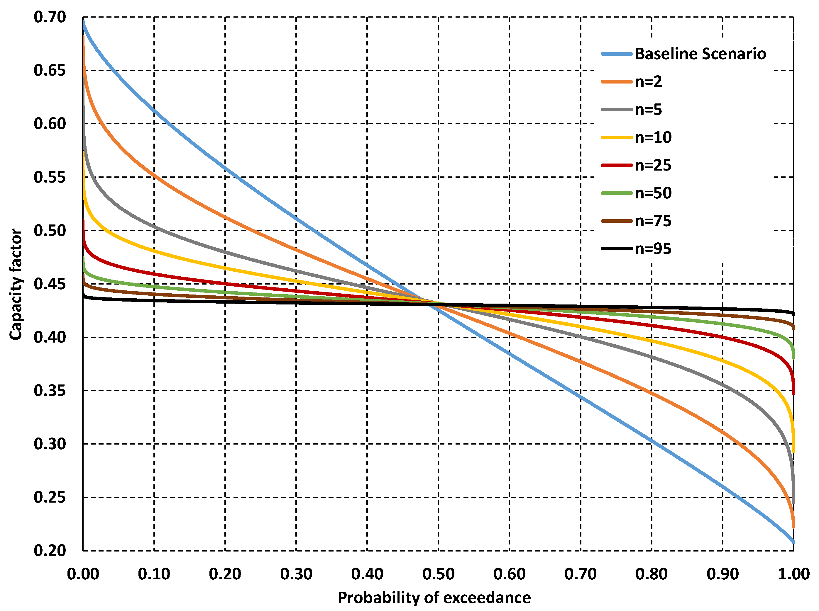Figure 9 contrasts the baseline scenario with arbitrarily chosen levels of wind turbine spatial dispersion.

The derived probabilistic curves allow for a better understanding of wind generation capabilities with respect to spatial dispersion. Within the MCS, spatial reliability signifies the combination of locations from the total sample that can guarantee a level of “joint” power production. Evidently, the output power variability decreases as more locations are accounted for (i.e., when turbine spatial distribution increases), revealing the tradeoff between guaranteed power output and spatial dispersion. The shape of the curves suggests that distributing wind turbines across a mix of regions with both strong and weaker generation potential improves the guaranteed power output. This is especially relevant for wind turbines since wind speed exhibits significant spatial variability. Hence, adequately distanced, and, as such, spatially decorrelated locations are expected to guarantee a greater aggregated power output than the one of centralized configurations; wind speed extremes (i.e., very low and high values) that inhibit generation in one location may be counterbalanced by increased generation due to favorable conditions in another one, a phenomenon which is not applicable when referring to centralized systems. Importantly, the observed range of capacity factors over Greece (i.e., from 0.20 to 0.70) emphasizes the significant spatial variability in wind resources compared to the solar ones, which show regular spatial patterns, which only ranged between 0.17 and 0.22 [12].

3.5. Scale–Reliability–Yield Laws for Wind Power

The tradeoff between guaranteed power output and turbine spatial dispersion is better presented when contrasting different probabilities of exceedance with respect to spatial dispersion. In this vein, the empirically derived capacity factor values are plotted with respect to the associated number of locations (which is a metric of spatial dispersion) for specific spatial probability values. The derived relationships exhibit asymptotic scaling laws that can be well approximated through the well-known Gompertz function. This function was initially proposed by Benjamin Gompertz in 1825 and is primarily used in demography and biology [53] to describe processes that start with exponential growth but then level off due to various constraints, such as limited resources. This feature makes it ideal for an accurate representation of spatial probability curve fitting since the curves’ inflection point (i.e., where growth is fastest) occurs at an early stage. As such, the empirical data, $CF$, for spatial probabilities of 80, 85, 90, 95, 97 and 99% are fitted (Figure 10) as follows:

$$CF=C{F}_{\infty }{e^{-bN}}^{-c}$$

(9)

where $C{F}_{\infty }$ is the theoretical maximum capacity factor value achieved under a fully distributed setting (which should be common for all spatial probabilities), and $b$ and $c$ are shape parameters that depend on the spatial dispersion metric, $N$. The shape parameters are inferred via calibration for each reliability level, underpinning that all spatial probability curves should converge to the asymptotic value, $C{F}_{\infty }$, when considering a full spatial dispersion. Consequently, these curves accurately capture the scale–reliability–yield relationship in wind power generation over the Greek region.

As indicated above, the shape of the curves suggests that increasing the spatial dispersion of turbines leads to increased guaranteed wind power yield. In contrast, for a given distribution setting, opting for a higher spatial reliability level leads to a decreased guaranteed yield. Remarkably, all curves converge to a $C{F}_{\infty }$ value of 0.47, which may be considered the optimal guaranteed wind power yield value under a fully distributed setting of “common” wind turbines across Greece. The use of the term “common” reflects the key assumption of considering the average capacity factor among a wide range of available technologies and their major design characteristic (i.e., hub height). Future technological advances, the substitution of old machinery and the anticipated development of offshore wind projects are expected to further boost this asymptote value.

In reality, Greece’s wind power production for the year of 2023 amounted to 10.92 TWh, a remarkable 20% of its total electricity demand (i.e., 53.7 TWh), while its installed capacity amounted to 5.23 GW, as documented by official sources [54,55]. By utilizing the aforementioned data, Greece’s capacity factor for wind installations in 2023 is calculated to be only about 0.24. Presumably, one would argue that a fully distributed setting can offer almost double the power output in comparison to Greece’s current wind projects. However, this (at first glance, surprisingly) large discrepancy between Greece’s theoretical wind power potential and its actual generation output mainly stems from the lack of large-scale energy storage and electrical transmission line interconnections, as well as from grid constraints (particularly, in non-interconnected islands). More specifically, during time periods when weather conditions are favorable for wind power generation, the demand load may be low, leading to extended power curtailments in order to avoid blackouts [56]. Notably, during 2024, system operators were forced to curtail 860 GWh of energy produced by renewables [57]. This finding is of significant importance for the overall strategic planning and management of energy projects at the national level.

3.6. Contrasting with Solar Power

As already mentioned, the spatial reliability concept has previously been investigated for the case of distributed solar PV energy [12], also resulting in scaling laws that express the reliable output power (in terms of mean annual $CF$) as a function of spatial dispersion via the use of Gompertz curves (Equation (9)). The derived probabilistic curves, expressing the asymptotic increase in $CF$ against the number of locations for different reliability levels are very similar to the wind case, yet they extend over a significantly limited range.

This is further revealed through Figure 11, which contrasts the 90% spatial reliability curves for the two major renewable sources, i.e., wind and solar PV, in Greece. Notably, when just 20 locations are accounted for, solar PV generation reaches its maximum guaranteed output for that given spatial probability, whereas wind power output indicates a continuously increasing performance, even beyond the maximum number of locations considered within this analysis, i.e., 100. When contrasting the fully distributed setting with the centralized one (i.e., for $N=1$), the gain in terms of $CF$ is 17% for wind energy, while it is less than 2% for solar energy.

These key differences are attributed to the much larger spatial variability in the wind process and its more complex conversion to output electrical power, with respect to solar radiation. Evidently, the asymptotic limits of the solar PV capacity factor (i.e., of the order of 19%) are substantially lower than in the case of wind energy due to the radically different physical and technical characteristics of the two renewable sources. Nevertheless, a very promising domain for further expansion of the issue of spatial reliability is its quantification under a joint-process context (i.e., solar and wind), which will also highlight the complementarity of the two most widely evolving renewable energy sources.

4. Discussion

Decentralized renewable-source-based power systems evidently offer a wide range of benefits when compared to centralized ones. These are not only restricted to a higher guaranteed yield, as demonstrated in this analysis, and lower transmission losses [23], but also span the security and resilience of energy infrastructure. In the recent era of geopolitical instability, irregular fluctuations in energy market prices across all scales, and climatic extremes, energy security is all the more relevant [58], with a disruption in centralized power systems and national grids often threatening to compromise the energy supply at the (trans)national scale. On the contrary, spatially dispersed systems may ensure the continuation of power supply, at least on a regional level.

From an energy management viewpoint, the application of the spatial reliability framework within wind power provides major improvements to the classical definition of guaranteed yield at the temporal dimension. By capitalizing on the spatiotemporal complementarity of wind patterns, a hypothetical system of spatially decorrelated turbines ensures continuous power generation, albeit sometimes at modest levels, when contrasted with the highly variable and intermittent output of centralized configurations. In fact, the distribution of wind turbines among any number of locations seemingly outperforms half of the centralized configurations in terms of guaranteed yield (Figure 9), debunking the common approach of opting for the “best”-performing location.

This work assesses wind potential through the novel concept of spatial reliability by utilizing the mean annual capacity factor as an overall performance metric over the area of interest. Actually, wind is driven by atmospheric processes that typically exhibit varying seasonality patterns, and thus is characterized by significant intra-annual variability [59]. Specifically, for the case of Greece, winter and early spring exhibit the highest generation output for most regions. On the contrary, during the summer months, wind generation becomes more location-dependent, with the Aegean regions benefitting from Etesian (Meltemi) winds, and the inland and western regions experiencing yield declines [60]. Hence, estimating spatial reliability on a monthly scale is expected to intensify generation output variability, especially during the summer months, further emphasizing the issue of spatial scale. As also revealed in the present analyses, this variability can be alleviated by expanding this framework to include the two most widespread renewable sources (i.e., wind and solar) considering their complementary nature [59,61,62].

To facilitate computations, which is an essential requirement under a Monte Carlo Simulation context, the wind-to-power conversion model follows the power curve rationale, as provided by the manufacturers. It is highlighted that this approach yields performance metrics that correspond to theoretically optimal conditions, in terms of micro-siting, to ensure optimal turbine placement, negligible wake losses, and effective turbine control, thus capturing the full spectrum of wind speed while minimizing hysteresis effects, as well as the ability to inject all produced power to the grid, thus avoiding curtailments. Yet, to actually account for all aforementioned issues in detail, a fully defined system should be available, which does not fall under the overall objectives of strategic planning exercises, where the concept of spatial reliability is applicable. In fact, the use of this concept is by definition site-agnostic since it is a statistical quantity referring to a sufficiently large region, not to a specific location.

With regard to wind projects’ planning, this analysis opted for selecting the candidate locations exclusively based on the overall wind regime (in terms of mean annual wind speed) to illustrate the benefits of a fully distributed setting. Consequently, further research on the location selection considering additional aspects of the wind process (e.g., seasonality, variability), technical constraints (i.e., regarding grid balancing, transmission issues, power regulations, etc.), socioeconomic aspects such as land availability, environmental conditions, and the visual impacts of wind turbines to landscapes, which is a determinant factor towards their wider social uptake [63,64].

In general, from an economic perspective, centralized large-scale power systems are deemed more cost-efficient both in terms of capital (e.g., site development, shared auxiliary infrastructure) as well as operational and maintenance costs due to economies of scale [23,65]. As such, a more detailed analysis is encouraged to investigate whether the gains in power output from decentralized settings, in financial terms, are sufficient to offset their generally higher implementation costs.

Lastly, this analysis revealed the significant difference between Greece’s theoretical generation potential and its actual yield. Acknowledging that this discrepancy is mainly attributed to the lack of sufficient energy storage components, an in-depth analysis on the historic trend of wind power curtailments in comparison to the evolution of installed capacity would serve as a strategic enabler towards targeted investments in energy storage components.

5. Conclusions

This work provided insights on the impact of spatial scale in wind power generation by verifying the recently introduced novel concept of spatial reliability within the wind sector. Contrary to solar PV energy, where this framework was initially demonstrated as a proof of concept, wind power is characterized by more significant variability not only due to the primary driver’s nature but also owing to machine-specific properties (turbine power curve) and design features (hub height).

The framework was applied to wind power over the Greek region. A detailed simulation procedure was formulated to estimate wind power output through an analytical equation that accounts for wind speed and turbine-specific characteristics (i.e., cut-in and rated wind speed, nominal power). In order to provide a universal metric to assess the under-the-scope locations’ generation capacity, the capacity factor was utilized. More specifically, acknowledging that spatial reliability refers to distributed systems across large regions, different technologies and design philosophies are expected to be applied. In this vein, the generation capacity of each region was derived from estimating the mean capacity factor of a large sample of wind turbines with different design features, which is considered to adequately capture a “common” turbine’s yield.

Subsequently, spatial probabilities for guaranteed wind power yield were quantified in a Monte Carlo setting by allotting a mix of turbine settings across combinations of representative well-performing locations. The locations’ “joint” generation output was then assessed and contrasted with that of centralized configurations. The probabilistic curves indicated that transitioning towards a more decentralized setting increases generation output variability while also increasing the guaranteed yield.

Finally, asymptotic-type scale laws were inferred to assess and quantify the relationship between spatial dispersion and guaranteed yield, revealing the tradeoff between these major metrics. The common asymptote of all curves corresponds to the theoretical maximum wind power yield, in means of the capacity factor, which is achieved under a fully distributed setting. Remarkably, the maximum capacity factor was found to be much larger (almost double) than the current capacity factor of wind power over Greece, mainly reflecting the significant power curtailments due to the lack of large-scale energy storage components.

In conclusion, the authors hope that the findings from this analysis will provide a compelling argument that will drive future investments in energy storage to make the most of current wind installations while also offering strategic guidance for the planning and development of future projects.