Article

Variable Dimensional Bayesian Method for Identifying Depth Parameters of Substation Grounding Grid Based on Pulsed Eddy Current

1
Baotou Power Supply Branch of Inner Mongolia Power (Group) Co., Ltd., Baotou 014030, China
2
School of Electrical Engineering, Chongqing University, Chongqing 400044, China
*
Author to whom correspondence should be addressed.
Energies 2025, 18(17), 4649; https://doi.org/10.3390/en18174649
Submission received: 14 July 2025 / Revised: 20 August 2025 / Accepted: 28 August 2025 / Published: 1 September 2025
(This article belongs to the Special Issue Reliability of Power Electronics Devices and Converter Systems)

Abstract

The substation grounding grid, as the primary path for fault current dissipation, is crucial for ensuring the safe operation of the power system and requires regular inspection. The pulsed eddy current method, known for its non-destructive and efficient features, is widely used in grounding grid detection. However, during the parameter identification process, it is prone to local minima or no solution. To address this issue, this paper first develops a pulsed eddy current forward response model for the substation grounding grid based on the magnetic dipole superposition principle, with accuracy validation. Then, a variable dimensional Bayesian parameter identification method is introduced, utilizing the Reversible-Jump Markov Chain Monte Carlo (RJMCMC) algorithm. By using nonlinear optimization results as the initial model and introducing a dual-factor control strategy to dynamically adjust the sampling step size, the model enhances coverage of high-probability regions, enabling effective estimation of grounding grid parameter uncertainties. Finally, the proposed method is validated by comparing the forward response model with field test results, showing that the error is within 10%, demonstrating both the accuracy and practical applicability of the proposed parameter identification method.

1. Introduction

In recent years, as the scale of power transmission and transformation projects continues to expand to meet the needs of the new power system, the number of substations has been increasing annually. The grounding grid, as a critical component of the substation, is primarily designed to efficiently direct fault current and lightning discharge current into the earth, ensuring the safety of equipment and personnel [1,2]. However, during actual construction, some grounding grids fail to meet design and operational requirements. Typical issues include key parameters, such as the burial depth of grounding bodies, not meeting the relevant standards [3,4,5], resulting in high grounding resistance that cannot effectively dissipate fault and lightning currents. In severe cases, this may jeopardize the safe and stable operation of the power system. Therefore, there is an urgent need for a fast and reliable method to detect key parameters of the grounding grid to enhance the operational safety and engineering efficiency of substation grounding systems [6,7].
The pulsed eddy current method, known for its excellent vertical resolution, especially its high sensitivity in detecting low-resistance conductors, has been widely used in underground metal target detection in recent years [8,9]. The substation grounding grid, as a typical good conductor, has a resistivity much lower than the surrounding soil medium. The electromagnetic field propagates more quickly through the soil than through the grounding conductor, which allows the pulsed eddy current method to provide high-layer resolution when detecting the grounding grid [10,11,12]. By obtaining high signal-to-noise ratio pulsed eddy current data, the underground structure of the substation grounding grid can be accurately determined through parameter identification. Parameter identification is the process of inferring the spatial distribution characteristics of underground targets based on observed data, and it is one of the most challenging aspects of pulsed eddy current measurements [13]. Common parameter identification methods include “smoke ring” rapid imaging, least squares method, and machine learning-based algorithms. Among them, the “smoke ring” method is an approximate analytical model based on the assumption of uniform half-space. Its depth inversion depends on the empirical coefficient and is sensitive to the dip angle of the anomalous body, so it is difficult to accurately reveal the depth information of the anomalous body [14,15]. The least squares method constructs a target function to measure the discrepancy between the observed data and the forward model, optimizing it numerically to improve detection efficiency and accuracy [16]. For instance, Wang [17,18] and Chen [19,20] used Differential Evolution (DE) algorithms to enhance the accuracy of parameter identification models. However, the Jacobian matrix will lead to too many conditions due to its ill-conditioned nature. This kind of global optimization algorithm usually has more iterations and poor real-time performance. With the advancement of computational power, machine learning applications in electromagnetic parameter identification have gained momentum. Thomas et al. used machine learning to quickly estimate the burial depth of underground metal materials [21] and further classified metal material types, achieving a recognition accuracy of 90% [22]. Li et al. [23] proposed a parameter identification method based on deep neural networks to reconstruct the electromagnetic response of underground targets, significantly improving the accuracy and computational efficiency of parameter identification. Although machine learning has the advantages of fast speed and high accuracy, it relies on a large number of high-dimensional training data and easily leads to data dimension disaster. At present, there are few practical application cases of the pulsed eddy current method in substation grounding grid detection, and data acquisition is more difficult. The non-training set distribution caused by substation grounding grid corrosion reduces its universality.
This study aims to achieve precise identification of underground substation grounding grids; thus, it proposes high requirements for the parameter identification algorithm, which must possess good global search capabilities and strong noise resistance. To address the non-uniqueness problem in parameter identification, as well as the limitations of traditional methods that only provide a single optimal solution and cannot assess parameter uncertainty, a study on electromagnetic data variable dimensional Bayesian probability parameter identification is conducted. Firstly, in the second section, an electromagnetic forward model suitable for substation grounding grid is constructed as the basis for subsequent parameter identification. Secondly, in the third section, considering the complex transformation characteristics of underground structures in different environments, the Reversible-Jump Markov Chain Monte Carlo (RJMCMC) algorithm is introduced, and the nonlinear optimization parameter identification results are used as the initial model. A two-factor control strategy is proposed to dynamically adjust the sampling step size, so as to enhance the sampling model’s ability to cover the high-probability region of the parameter space and realize the effective estimation of the model parameter uncertainty. Finally, the feasibility and effectiveness of the proposed method in substation grounding grid detection are verified by the model and field test in Section 4 and Section 5, which shows that the method has good performance in dealing with non-uniqueness and noise interference.

2. Electromagnetic Forward Model of Substation Grounding Grid

2.1. Construction of Electromagnetic Forward Model

When using the pulsed eddy current method to measure the substation grounding grid, it can be considered as an underground low-resistance anomaly. Through steps such as noise reduction and parameter identification, the underground anomaly can be effectively recognized [24]. Due to the different resistivity and thickness between the underground grounding grid and surrounding mediums, the resistivity and thickness of each layer are set as ρi and hi, respectively, as shown in Figure 1. The buried grounding grid is regarded as one layer in the layered model.
In this study, both the transmitting and receiving coils are circular. The coils are designed with circular symmetry, i.e., a central return loop structure, which simplifies the mathematical description and modeling process for forward modeling and parameter identification. The central return loop source device consists of two coils, used as transmitting and receiving magnetic dipoles, respectively. The electromagnetic field components excited by the vertical magnetic dipole source are TE (Transverse Electric)-type fields. The TE, TM (Transverse Magnetic) fields, and the properties of the geological layers differ. The electric field in the TE-type field is parallel to the layer plane, with a strong penetration ability through high-resistance layers and minimal anisotropic influence from the layers. In this paper, a magnetic source is used to detect the grounding system.
At this point, the electromagnetic potential function F is introduced, which conveniently represents the electric field E and the magnetic field H. In the coordinate system of Figure 1, the potential function F of a single magnetic dipole is given by the following expression:
F ( r , z ) = m 4 π 0 e u i z + h + r T E e u i z h λ u i J 0 ( λ r ) d λ
where m represents the magnetic moment of the dipole, J0(λr) is the zeroth-order Bessel function, indicating the diffusion of the magnetic field in space, λ is the integration variable, describing the propagation characteristics of the electromagnetic field in space. λ = k x 2 + k y 2 , kx and ky represent the wave numbers in the x- and y-directions, respectively. u n = λ 2 k n 2 , kn2 represents the wave numbers of the n-th layer, and u0 represents the permeability of air. The variable r is the radial distance from the source to the receiver, z is the vertical coordinate for the layered medium, and rTE is the reflection coefficient. The coil is radially divided into numerous tiny current loops, and each loop is regarded as a magnetic dipole (the magnetic moment mis proportional to the current I and the area). By integrating (1) within the range of radius a and using the recurrence relation of Bessel functions, (2) containing the first-order Bessel function J1(λr) is finally obtained:
F ( r , z ) = I a 2 0 1 u i e u i z + h + r T E e u i z h J 1 ( λ a ) J 0 ( λ r ) d λ
where J1(λr) is the first-order Bessel function used to describe the current distribution in the return loop source. In cylindrical coordinates, when located on the ground surface (i.e., z = 0, h = 0), the magnetic field and electric field generated at the center of the horizontal central return loop transmitting coil are expressed as follows:
E φ = i ω μ F r = z 0 I a 2 0 1 + r T E λ u 0 J 1 λ a J 1 λ r d λ H r = 2 F r z = I a 2 0 1 r T E λ J 1 λ a J 1 λ r d λ H z = 1 r F r ( r F r ) = I a 2 0 1 + r T E λ 2 u 0 J 1 λ a J 0 λ r d λ
where z 0 = i ω μ 0 . At the ground surface (z = 0), in the expressions of the magnetic field Hz and the electric field E at the center of the horizontal loop coil, the reflection coefficient rTE directly reflects the difference in electromagnetic characteristics between the underground media (soil and grounding grid); the grounding grid, as a low-resistivity body, will increase the modulus of rTE, resulting in an increase in the rate of change in the magnetic field amplitude in Equation (3). The reflection coefficient rTE is calculated as
r TE = λ u ^ 1 λ + u ^ 1
When the magnetic source serves as the excitation source, Equation (4) can be transformed into
r T E = Y 0 Y 1 ^ Y 0 + Y 1 ^
In Equation (5), Y0 and Y 1 describe the propagation impedance of the electromagnetic field in the layered medium, which can be obtained by the recursive relationship in Equation (6):
Y 0 = u 0 z 0 Y 1 = Y 1 Y 2 + Y 1 tanh u 1 h 1 Y 1 + Y 2 tanh u 1 h 1 Y n = Y n Y n + 1 + Y n tanh u n h n Y n + Y n + 1 tanh u n h n Y n = Y N = u n i ω u 0
To simplify the calculations, only the center point of the received component is considered, where r = 0, while J0(0) and J1(0) are 1 and 0, respectively. The electromagnetic field expression at the center location is
E ϕ = 0 H r = 0 H z = I a 2 0 [ 1 + r T E ] λ 2 u 0 J 1 ( λ a ) d λ d B z ( ω ) d t = i ω μ 0 I a 2 0 [ 1 + r T E ] λ 2 u 0 J 1 ( λ a ) d λ
The magnetic field at the center point, denoted as Hz, is the frequency-domain response Hz(ω). Since the measurement of the pulsed eddy current method primarily involves parameter identification based on induced electromotive force, the derivative of Hz(ω) with respect to time gives the fourth term in Equation (7). To obtain the time-domain electromagnetic field response, a Fourier transform of Equation (7) is performed. During the derivation process, the Fourier transform is converted into the integral of high-oscillation sine and cosine functions as follows:
f c ( k ) = 0 + F ( x ) cos ( k x ) d x f s ( k ) = 0 + F ( x ) sin ( k x ) d x
In Equation (8), due to the high oscillation of sin(kx) and cos(kx), the numerical solution obtained by approximate integration often does not meet the required precision. Researchers have found that for most practical problems, including the substation grounding grid in this study, electromagnetic response cannot be directly solved by an analytical solution, and numerical integration methods are required in the forward calculation process. For example, due to the oscillatory nature of Bessel functions, especially at relatively high wave numbers, numerically performing the integration is extremely complex. A commonly used approach nowadays is to carry out approximate calculation through the fast Hankel transform.
After obtaining the frequency-domain solution of the vertical magnetic field, the usual practice is to obtain the time-domain solution by converting the digital filtering operator. This paper first uses the filter coefficients from the Hankel transform of the first-order Bessel function to calculate the electromagnetic signal in the frequency domain [25]. The calculation expression is as follows:
f ( r ) = 1 r i = 1 n K ( λ i ) W i λ i = 1 r 10 [ a + ( i 1 ) s ] , i = 1 , 2 , , n
where i represents the sampling point location and Wi is the filter coefficient. From Equation (7), it is known that linear computation of the first-order Bessel function is required, with n = 140, a = −7.91001919000, and s = 8.7967143957 × 10⁻². Using the above expression, the electromagnetic signal in the frequency domain can be calculated.
After calculating the frequency-domain signal, since the subsequent signal processing in this paper involves time-domain signal processing, it is necessary to convert the frequency-domain signal into a time-domain signal. By using the sine and cosine transform method, the frequency-domain signal Hz(ω) is transformed into a time-domain signal, and the expressions for the vertical magnetic field time-domain signal and the derivative of the magnetic field in terms of the sine–cosine transform are as follows:
H z ( t ) = 2 π 0 I m [ H z ( ω ) ] 1 ω cos ( ω t ) d ω = H z ( 0 ) 2 π 0 R e [ H z ( ω ) ] 1 ω sin ( ω t ) d ω H z ( t ) t = 2 π 0 I m [ H z ( ω ) ] sin ( ω t ) d ω = 2 π 0 R e [ H z ( ω ) ] cos ( ω t ) d ω
The time-domain signal can be obtained by the sine transform method as follows:
f s ( t ) = 1 t π 2 n = N 1 N 2 F ( ω ) c sin ( n Δ )
where Δ is the sampling interval and csin() is the transform filter coefficient, discretizing ω = e/t and substituting it into the electromagnetic field response in the frequency domain for calculation. Finally, the response V(t) at the center of the layered earth model for the central return loop device is
V 1 ( t ) = q μ 0 H z ( t ) t
where μ0 represents the permeability of free space, and q is the equivalent area of the excitation coil. After the central return loop generates an electromagnetic signal through the magnetic source, the magnetic field response from the grounding grid is collected by the receiving coil. The induced voltage V1(t) of the receiving coil is proportional to the time derivative of the magnetic field (∂Hz/∂t), and the burial depth of the grounding grid will affect the diffusion speed of the magnetic field: the greater the burial depth, the longer the time delay for the magnetic field to reach the ground surface. An increase in the number of turns n of the coil and the effective area S in (12) will increase the amplitude of V1(t). Essentially, this corresponds to obtaining the transfer function of the earth. The collected signal is expressed as the induced voltage form V2(t):
V 2 ( t ) = n d φ d t = n S d B d t
In Equation (13), n and S are the number of turns and effective area of the receiving coil, respectively, and B is the magnetic flux density along the axis of the receiving coil. In the parameter identification algorithm, the relationship between the induced voltage signal collected by the receiving coil and the induced voltage signal calculated by the forward algorithm is used to determine the structure of the underground medium.

2.2. Verification of Forward Model

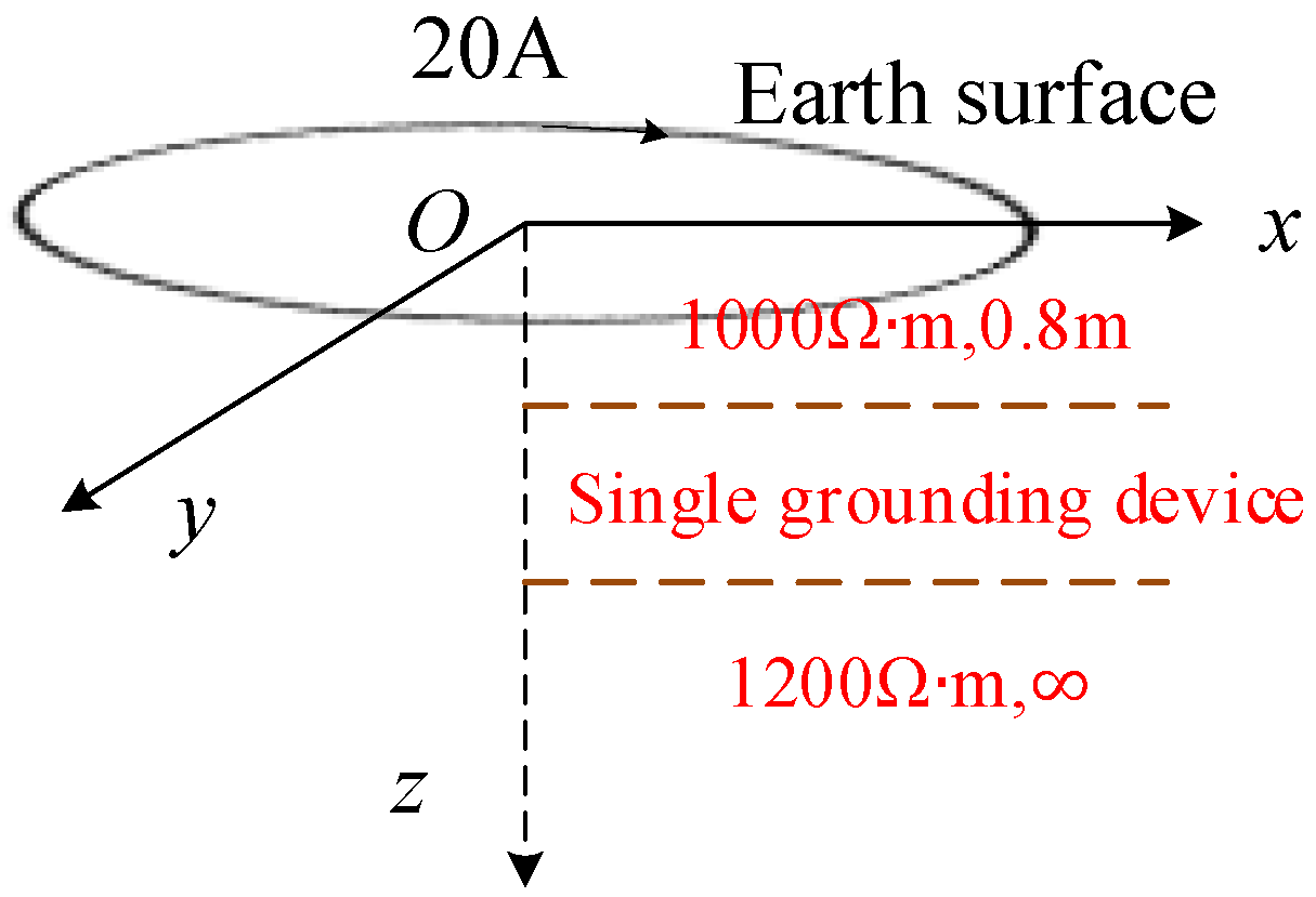
An H-type model for the substation grounding grid is constructed, where the resistivity of the middle layer, representing the substation grounding grid, is significantly lower than the resistivity of the upper and lower soil layers, as shown in Figure 2. The model parameters are set as listed in Table 1. The excitation current amplitude is set to 20 A, with the number of turns for the transmitting coil set to 10 and a radius of 0.4 m. An H-type model for the substation grounding grid is constructed, and its specific structure is shown in Figure 2. The model divides the underground structure of the grounding grid into three layers, which are soil, grounding grid, and soil from bottom to top. The settings of various parameters of the model are detailed in Table 1, where Resistivity represents the resistivity of each layer, Thickness represents the thickness of each layer, and ρ2 and h2 correspond to the resistivity and thickness of the grounding grid, respectively. The basis for determining the parameter values is explained as follows: The main material of the grounding grid is galvanized steel, whose conductivity is usually 1 × 10⁶ S/m or higher. Considering that this conductivity value is significantly different from that of soil, and when the conductivity is greater than 1 × 10⁶ S/m, it has little impact on the calculation results, 5.6 × 10⁶ S/m is selected in this paper for conversion to determine ρ2. In addition, the thickness h of the grounding grid is set to 0.012 m, which is in line with the conventional value range for grounding grid design in China. The excitation current amplitude is set to 20 A, with the number of turns for the transmitting coil set to 10 and a radius of 0.4 m.
The number of turns for the receiving coil is set to 100, with a radius of 0.1 m. The resulting forward modeling results are shown below.
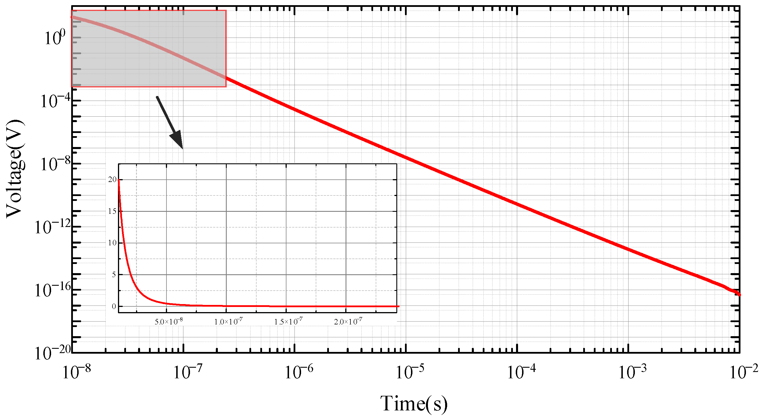
Figure 3 shows the variation in the pulsed eddy current signal during the grounding grid detection process, plotted on a logarithmic scale. The inset uses a linear scale for the x-axis and a logarithmic scale for the y-axis to facilitate observation of early response details. In the H-type geo-electric model, due to the resistivity of the layers exhibiting a high–low–high variation trend, the pulsed eddy current response curve shows a fast–slow–fast attenuation pattern. However, because the grounding grid being detected in this study is very small, the attenuation variation trend is not very obvious, and the dynamic range is extremely large. This further increases the difficulty of parameter identification. In common parameter identification algorithms, it is even possible for the grounding grid to be overlooked. Therefore, in the parameter identification algorithm used in this paper, prior information from the grounding grid design is incorporated through additional conditions to assist the parameter identification process.

3. Substation Grounding Grid Parameter Identification Method

The goal of pulsed eddy current parameter identification is to estimate the model parameters m that best fit the real conditions of the grounding grid based on the observed data d. However, due to the uncertainty of the observed data, parameter identification is often challenged by non-uniqueness and data errors caused by noise. Even with the same observed data, multiple reasonable underground structural models may correspond, making it difficult to fully describe model uncertainty by relying solely on traditional least squares fitting or regularization methods. To more reasonably characterize the uncertainty in the parameter identification results and fully utilize available geological information, Bayesian parameter identification is introduced, as shown in the following equation:
P ( m | d ) = P ( d | m ) P ( m ) P ( d )
Under the Bayesian parameter identification framework, the solution for the geoelectric model parameters m follows Bayes’ theorem, where the posterior probability distribution P(m|d) is estimated given the observed data d. Here, P(m|d) represents the posterior probability distribution, which evaluates the probability of each possible geoelectric model m after measuring the electromagnetic data d. This is the primary goal of Bayesian inference. P(d|m) is the likelihood function, which describes the probability of observing the electromagnetic data d given the geoelectric model m, indicating how well the model fits the observed data. P(m) is the prior distribution, reflecting the prior expectations of the model parameters before incorporating the observed data. In this paper, the prior information is constrained based on national standards and field measurement data. P(d) is the marginal likelihood, which serves as the normalization factor to ensure the posterior probability density is normalized. Its value is calculated by integrating over all possible geo-electric models’ contributions to the data d, as shown below:
P ( d ) = P ( d | m ) P ( m ) d m
The Bayesian parameter identification method optimizes and constrains the model parameters by combining prior information with the degree of fit to the observed data, operating within a probabilistic statistical framework. In the identification of depth parameters of substation grounding grids, the strong non-uniqueness of geophysical parameter identification makes it difficult for a single optimal solution to fully reflect model uncertainty. However, the Bayesian method can quantify uncertainty by providing the probability distribution of model parameters, thereby improving the robustness and physical interpretability of the results. Nevertheless, in the practical application of electromagnetic identification, the Bayesian method has two main problems.
First, the calculation of the posterior probability distribution is difficult. The posterior probability is derived from the product of the prior distribution and the likelihood function, and needs to be normalized over the entire model space, which involves high-dimensional integration and is usually difficult to solve analytically. The electromagnetic parameter identification process in this paper also has nonlinear and high-dimensional characteristics, so a sampling method instead of integration is adopted, and a large number of statistical samples are used to approximate the optimal solution. Second, sample generation is difficult. To approximate the posterior probability distribution, a large number of samples need to be generated from the model parameter space. The common Markov Chain Monte Carlo (MCMC) method can extensively and randomly search for model parameters based on prior information and generate predicted data close to the observed data. However, when directly applied to high-dimensional spaces, its efficiency is extremely low. Moreover, the traditional MCMC method has a fixed parameter dimension, which makes it difficult to adapt to changes in the number of layers and interface positions in the grounding body model. To address these issues, the Reversible-Jump Markov Chain Monte Carlo (RJMCMC) method has been introduced. This method enables dynamic adjustment of the dimensions of model parameters (such as the number of layers and interface positions) through jump sampling between different dimensions, thereby exploring the possible model space more efficiently and obtaining a posterior probability distribution more consistent with the observed data. It effectively improves sampling efficiency and enhances the accuracy of complex Bayesian parameter identification.

3.1. Model Parameter Initialization

In the electromagnetic model of the substation grounding grid, the key model parameters mainly include resistivity, number of layers, and interface depth. The initial model can either be specified by the user or randomly generated based on certain rules. A reasonable initial model setup helps to start sampling from a parameter space that is closer to the true solution, thus effectively reducing the number of ineffective samples during the early stages of the MCMC algorithm.
Since MCMC sampling often starts from models with low posterior probability, it requires numerous iterations to gradually approach high-posterior regions. This phase is known as the burn-in phase. The length of the burn-in phase is influenced by multiple factors, including the complexity of the substation grounding grid parameter identification problem, the quality of the initial model, sampling strategy, and convergence criteria. Selecting a more reasonable initial model can significantly shorten the burn-in process and improve overall parameter identification efficiency.
In this study, prior to parameter identification, an optimized strategy is introduced to construct an approximately high-quality initial model to accelerate the convergence process during the burn-in phase. It should be emphasized that this initial model is only used to optimize sampling efficiency and is not intended to serve as the final parameter identification solution. Inspired by the “snow ablation” mechanism in the Snow Ablation Optimizer (SAO), which exhibits a good balance between global search and local exploitation (Exploration and Exploitation, ENE), this approach can generate an initial solution that is closer to the true model distribution, thereby improving the overall efficiency of the RJMCMC sampling process.

3.2. Prior Function and Likelihood Function Generation

In Bayesian parameter identification, the prior function and likelihood function are central to the calculation of the posterior probability distribution. They collectively determine the estimated results of the model parameters.
(1)
Prior Function
During the model parameter setting process, parameter thresholds need to be set based on prior information. For the resistivity search range, it is typically set based on known geological information, as different substation grounding grids have varying resistivity ranges for soil environments. Constraints are applied to resistivity, the number of layers, interface depth, and noise-influenced parameters:
(1) Minimum and maximum model layers (kmin, kmax).
(2) Minimum and maximum interface depth (zmin, zmax).
(3) Minimum and maximum resistivity (ρmin, ρmax).
(4) Noise impact range dn(dnmin, dnmax).
During model perturbation, except for the noise impact, the remaining prior information uses logarithmic parameters to ensure that all parameters are positive and that their perturbation range is more flexible. Given that the characteristics of these four parameters differ, the prior probability calculation should be performed by distributing the calculation, expressed as
p ( m ) = p ( k ) p ( z | k ) p ( ρ | k ) p ( d n )
Compared to conventional underground model measurements, the object of detection in this paper is the substation grounding grid. Therefore, a fixed parameter layer can be set, where the thickness and resistivity of the grounding grid are predetermined. In this case, p(k) is not affected by the layer of the underground grounding grid and is still considered a bounded uniform distribution:
p ( k ) = 1 k max k min + 1 , k min k k max
Before performing signal parameter identification, the surface resistivity can first be estimated via parameter identification. The surface resistivity ρ0 measured at this point can be used as the initial mean to construct a Gaussian distribution. A weight parameter is introduced to adjust the influence of the prior distribution on the final parameter identification results. The expression for p(ρ|k) is as follows:
p ρ | k = 1 2 π k C ρ 1 2 exp ω 2 ( ρ ρ 0 ) T C ρ 1 ρ ρ 0
where ω is the weight parameter. The larger ω is, the stronger the influence of the prior distribution, and the parameter identification results will tend to align with the prior information. Conversely, smaller ω values rely more on the observed data. is the variance matrix of the resistivity prior information, which is a diagonal matrix, with Cρ = diag(log(1 + ρr)2). Due to the existence of the grounding grid, the magnitude difference between resistivities is vast, so logarithmic operations are used in the calculation. When the number of layers k is determined, there are k! ways to arrange each layer’s interface at selected depths. Because of the grounding grid, its thickness and distribution can be considered a fixed value, and thus, p(z|k) in this section can be modified as
p ( z | k ) = 1 Δ z k 1 , z min z i z max , i = 1 , 2 , , k
where Δz is the layer thickness, and noise signals are assumed to follow a uniform distribution:
p ( d n ) = 1 d n max d n min , d n min d n d n max
Given the presence of the underground grounding grid, the number of initial model layer interfaces for parameter identification must be at least 2, i.e., there must be 3 layers underground.
(2)
Likelihood Function
In Bayesian parameter identification, the likelihood function primarily serves to assess the degree of fit between the candidate model m that generates the data dmodel and the actual observed data d. The higher the likelihood value, the better the model fits the observed data. After electromagnetic data denoising, errors due to measurements and prior signal processing can be considered Gaussian, and the likelihood function can be expressed as:
p d | k , z , ρ , d n = 1 2 π N d C d exp ω 2 d f ( m ) T C d 1 d f ( m )
where d represents the observed data, f(m) is the forward operator, and Cd is the prior variance matrix. The diagonal elements of Cd represent the measurement uncertainty, i.e., variance, and it is assumed that the data errors are independent. The larger Cd is, the greater the measurement error. In such cases, the impact of prior information should be increased, and thus, a weight factor ω is added to control the influence of prior information on sample generation. Nd represents the number of observed data points.

3.3. RJMCMC Method Improvement

When the number of layers in the subsurface is determined or the underground structure is simple, the samples generated by MCMC at the theoretical level can identify a set of optimal grounding grid models to simulate the underground structure. However, due to the large magnitude difference between the resistivity of the grounding grid and other underground media, simply dividing the underground structure into three layers can easily lead to multiple high-quality solutions, which do not meet the required results for parameter identification, as described in Section 2. Furthermore, if the outdoor measurement environment is complex, such as in mountainous areas, it significantly reduces the measurement accuracy. Therefore, during the sampling process, the number of samples produced in the initial stage should be as rich as possible, and during the iterations, the number of layers and the location of interfaces in the model should be adjusted based on the results. The RJMCMC sampling process is similar to MCMC, but RJMCMC allows sampling to jump between different model dimensions to better explore the underground model of the grounding grid.
The main purpose of RJMCMC sampling is to find an optimal underground electrical model that best fits the observed data. However, due to the non-uniqueness of geophysical parameter identification, there are usually multiple possible models that can explain the same data. Therefore, the goal of this paper is not to find a unique solution but to sample from all possible models and ultimately select the model set that best fits the observed data. RJMCMC introduces a dimensionality-changing mechanism, allowing the model to freely jump between different model spaces, thus flexibly searching for the optimal solution. Additionally, to improve sampling accuracy and efficiency, a dual-factor (ω-c) is introduced to enhance the resolution of resistivity and dynamically control the sampling step size.
(1)
Model Generation Based on Dual-Factor Control
Based on the horizontal layered model of the grounding grid, an iterative method using dual-factor control (ω-c) is proposed, which controls the weight of prior information and the step size of sampling to construct a complete electromagnetic data distribution model. In the proposal distribution sampling stage, candidate models are built for the three main parameters of parameter identification (resistivity, interface depth, and number of layers). Candidate models are typically generated in the following two ways: RJMCMC uses the Birth/Death mechanism to adjust the number of layers and the depth of interfaces; after determining the number of layers and interfaces, the resistivity for each layer is adjusted. Therefore, the proposal distribution function q(m′|m) in the RJMCMC sampling process consists of the following three parts:
q ( m | m ) = q ( k | k ) q ( z | k , z ) q ( ρ | k , z , ρ )
where q(k′|k) controls the change in the number of layers through the Birth/Death mechanism, q(z′|k′, z) controls the adjustment of the interface depth after the number of layers is determined, and q(ρ′|k′, z′, ρ) controls the adjustment of resistivity. The update of the resistivity parameter is determined by the proposal distribution and follows a Gaussian distribution. That is, the new resistivity value is randomly drawn from a Gaussian distribution with the current model’s resistivity as the mean. Therefore, except for the grounding grid layer, the expression is similar to that in the prior Equation (18).
q ρ | k , z , ρ = 1 2 π k C ρ k k , z 1 2 exp 1 2 ρ k ρ k k , z T C ρ k k , z 1 ρ k ρ k k , z
where ρk represents the resistivity of the candidate model, and the mean vector ρ k k , z is the resistivity of the current model, both of which are calculated logarithmically. C ρ k k , z is the posterior covariance matrix, which is typically linearized from the posterior model variance:
C ρ k k , z ω C ρ 1 + J T C d 1 J 1
Here, J is the sensitivity matrix, representing the impact of model parameter changes on the observed data, thus adjusting the sampling step size for model parameters. If a particular value in the matrix is large, it indicates that changes in that resistivity significantly affect the observed data, making the parameter identification result sensitive to this parameter. The physical meaning of ω is consistent with the likelihood function (21), used to balance the weight between model constraints and data fitting. The sampling step size is controlled by the posterior covariance matrix, with a scaling factor c dynamically adjusting the step size:
C ρ k k , z = c × C ρ k k , z
where c is a dynamic factor constructed by sine and cosine functions, which is used to control the scaling of the sampling step size, which equals c1 plus c2, as shown in (26).
c 1 = sin 3 π i t T + 1.5 c 2 = cos 3 π i t T + 1.5
At this point, RJMCMC updates the model in four ways:
(1) Layer Addition (Birth Move): Here, k′ = k + 1, and a random position is chosen between the minimum depth zmin and maximum depth zmax as the new interface. This interface follows a uniform distribution U(zmin, zmax) and forms a new layer. The resistivity of this layer follows a normal distribution N(ρ, σbirth2), where ρ is the resistivity of the current interface.
(2) Layer Deletion (Death Move): Here, k′ = k − 1, and a layer is randomly removed from the geo-electric model.
(3) Layer Perturbation (Perturbation Move): A random layer interface is selected for a position change, with the change step size following a normal distribution N(0, σmove2).
(4) Resistivity Update (Resistivity Change): Here, k= k, z= z, and only the resistivity is updated, with the change step size following a normal distribution N(ρ, σchange2), where ρ is the current resistivity of the interface.
It should be noted that since the thickness and resistivity of the grounding grid are much smaller than those of the generated model, during model update, it is first checked whether the layer thickness is greater than or equal to 0.1, and whether the resistivity is greater than 0 (logarithmic form is used in the calculation). In the model changes above, the update mode is chosen by randomly generating a number between 0 and 1 to satisfy the following condition:
q ( k | k ) = 1 6 , k = k + 1 ( Birth ) 1 6 , k = k 1 ( Death ) 1 6 , k = k ( Perturbation ) 1 2 , k = k ( Change )
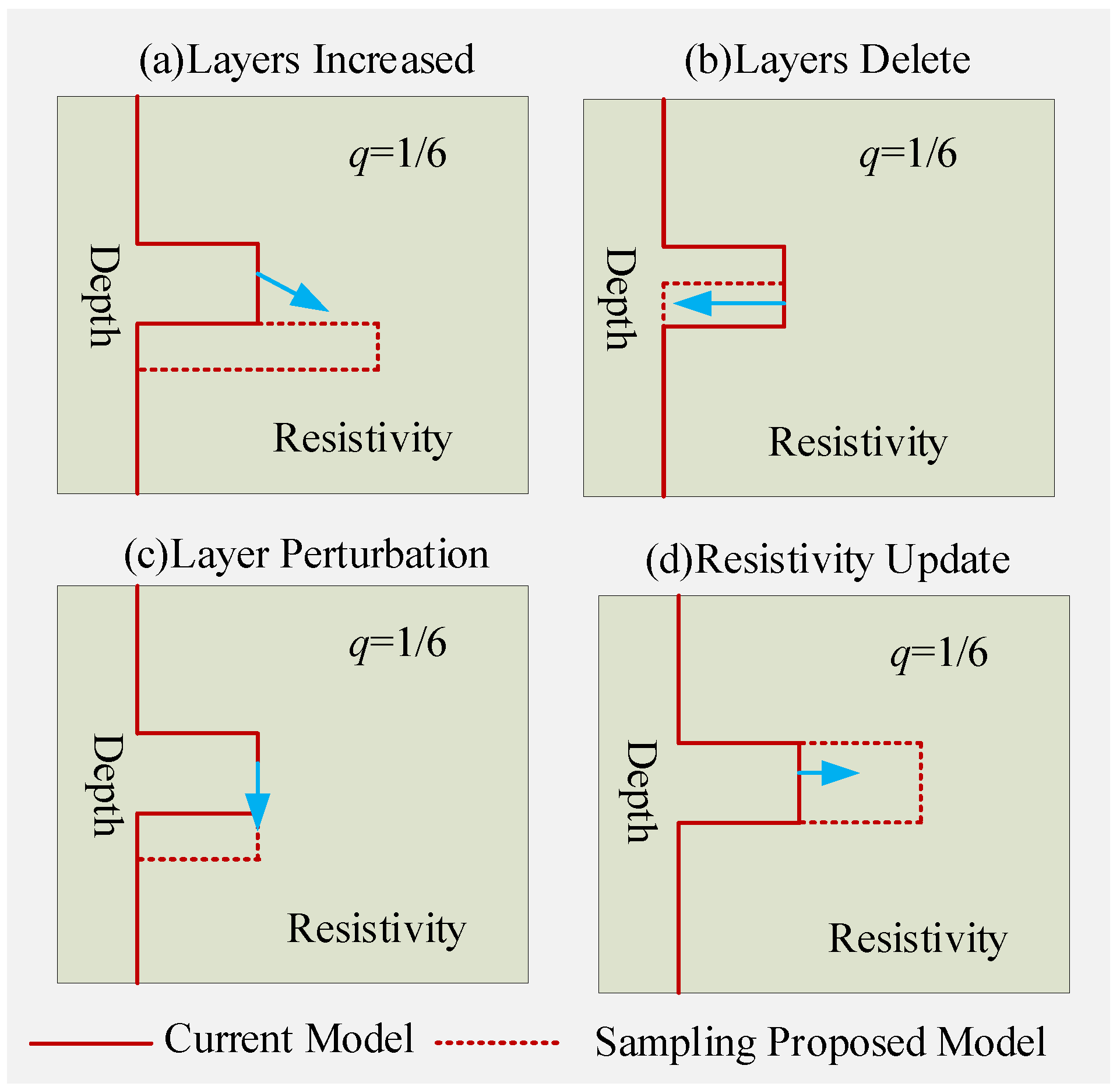
Because the changes in the number of layers and interface depth significantly impact the model, excessive frequency of layer adjustments during sampling may prevent RJMCMC sampling from converging. Excessive interface perturbations could lead to model instability. Therefore, the sampling probabilities for the first three disturbance types (Birth, Death, Perturbation) are set to 1/6, preventing overly frequent adjustments in the number of layers. The probability for resistivity updates is increased to 1/2 to optimize the resistivity distribution while keeping the number of layers fixed. The schematic of state changes is shown below:
Figure 4 demonstrates the four possible states of the new model generated by RJMCMC sampling: (a) layer addition, (b) layer deletion, (c) layer perturbation, and (d) resistivity update. However, not all generated models are suitable for sampling data. Therefore, during the sampling process, each generated model is evaluated for its applicability based on a probability model. This process ensures that the model reasonably fits the observed data and improves the stability and reliability of the parameter identification results.
(2)
Model Acceptance Probability Setup
Whenever a model is generated, an acceptance–rejection parameter needs to be set to determine if the model should be accepted. According to the Metropolis–Hastings sampling concept, the acceptance probability α(m′|m) is calculated as follows:
α ( m | m ) = min 1 , p d | m p d | m p m p m q m | m q m | m J
where J is the Jacobian matrix; in this paper, |J| is set to 1 to ensure that the transformation between different dimensions meets the invertibility requirement. The terms p(d|m′)/p(d|m), p(m′)/p(m), and q(m|m′)/q(m′|m) are the likelihood ratio, prior probability ratio, and proposal probability ratio, respectively. The prior probability ratio and likelihood ratio are calculated using Equations (16) and (21). The proposal probability ratio measures the probability of transitioning from the current model m to the candidate model m′ and is calculated as
q m | m q m | m = Δ z 2 π σ birth k + 1 exp ρ ρ 2 2 σ birth 2 , Birth k Δ z 2 π σ death exp ρ ρ 2 2 σ death 2 , Death 1 , Perturbation 1 , Change
A random number ξ between 0 and 1 is generated. If ξ is smaller than the value of Equation (28), the model is accepted; otherwise, it is rejected, and a new candidate model is generated for sampling, continuing until convergence or the maximum sampling threshold is reached.

3.4. Convergence Criterion for Uncertainty Assessment

To avoid the use of excessive computational resources, we define the sampling convergence condition as being reached when the model’s credible interval and the standard deviation of the error’s standard deviation remain sufficiently stable during the sampling iterations. The stability condition for the model’s credible interval is set as follows:
C R ( S i ) C R ( S i S 0 ) C R ( S i ) < k 1 %
where CR(x) is the boundary value of the credible interval for the x-th sampling, Si is the current cumulative number of samples, excluding the burn-in phase samples, and S0 is the pre-set interval of sampling. The physical meaning behind Equation (30) is that when the fluctuation of the model’s credible interval range for the Si-th sampling, compared to the credible interval range of the previous S0 samples, is less than k1%, it can be considered that the model’s credible interval stability condition has been achieved.
The stability condition for the standard deviation of the error’s standard deviation is, specifically, that the system computes the statistical characteristics of the model fitting error every N_refresh iterations and maintains a sliding window N_end during the sampling process to record the root mean square (RMS) error for the most recent N iterations. Let the error samples in the sliding window be {RMS1, RMS2, …, RMSN}; then, the corresponding error standard deviation is
σ R M S = 1 N 1 i = 1 N ( R M S i R M ¯ S ) 2
The system further monitors the fluctuation of the error standard deviation across multiple cycles. Let σRMS calculated over the past several cycles be {σ1, σ2, …, σN}. The standard deviation of these standard deviations is defined as
σ s t d = 1 M 1 j = 1 M ( σ j σ ¯ ) 2
where M = N_end/N_refresh. When σstd is smaller than a pre-set threshold δ, it is considered that the sampling process has entered the stable phase, signaling the “end of sampling.” In addition, to prevent sampling from getting stuck in low-posterior regions and causing prolonged ineffective sampling, the system sets an upper limit for the number of consecutive rejected models. Once this limit is reached, the sampling process is automatically interrupted to avoid wasting computational resources.
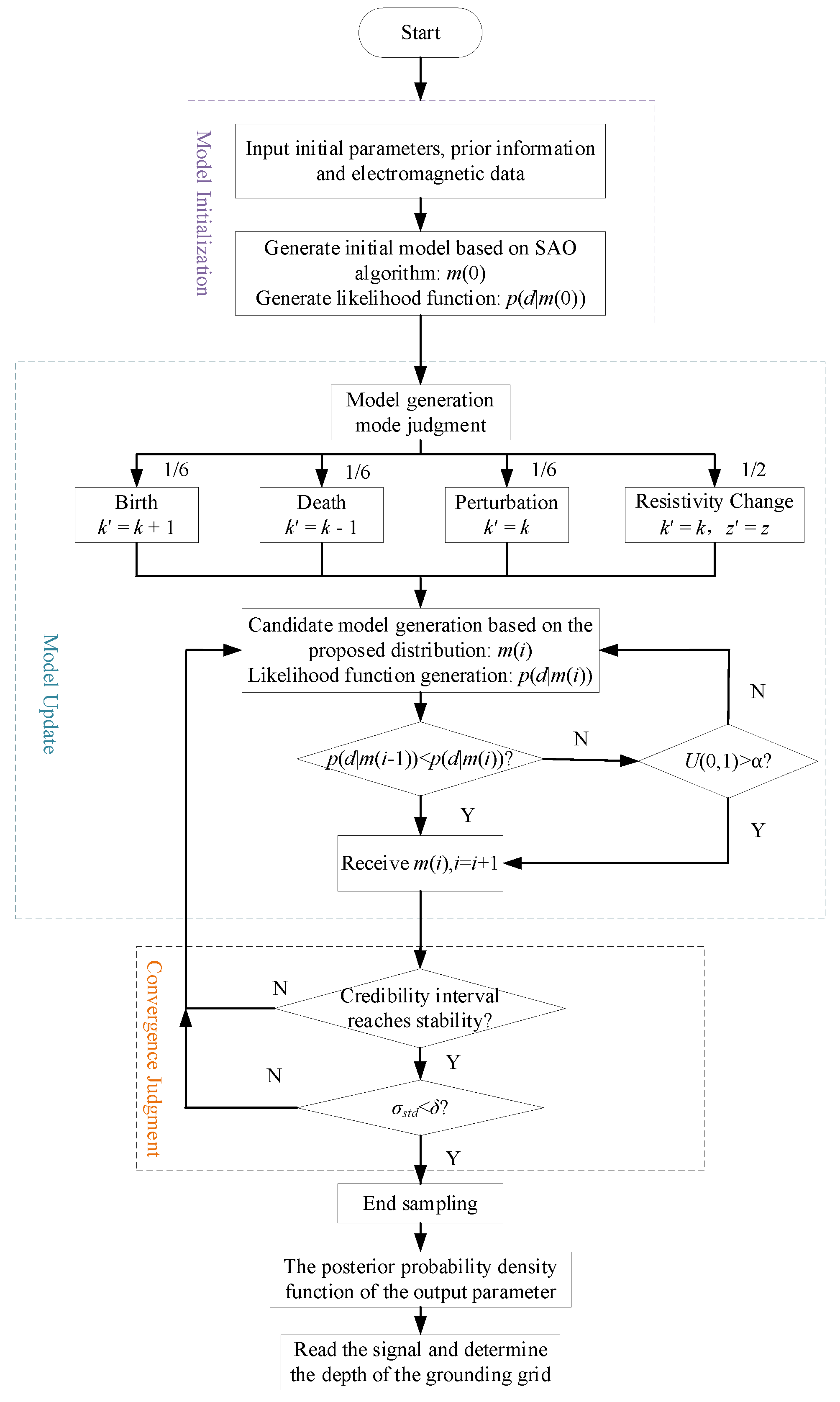
Based on the above analysis, the dimensional Bayesian flowchart is shown in Figure 5.

4. Simulation Model Verification of Parameter Identification

4.1. Parameter Identification Results for the H-Type Grounding Grid Model

The central return loop device is used to perform forward analysis on the H-type grounding body model, as shown in Figure 2. Gaussian random noise with a 5% amplitude ratio is added to the forward results to simulate real-world data. Dimensional Bayesian parameter identification is then performed, with parameter settings as shown in Table 2. All model training and testing were conducted on a workstation equipped with an NVIDIA RTX 3090 GPU (24 GB VRAM), an Intel i9-13900K CPU, and 64 GB RAM.
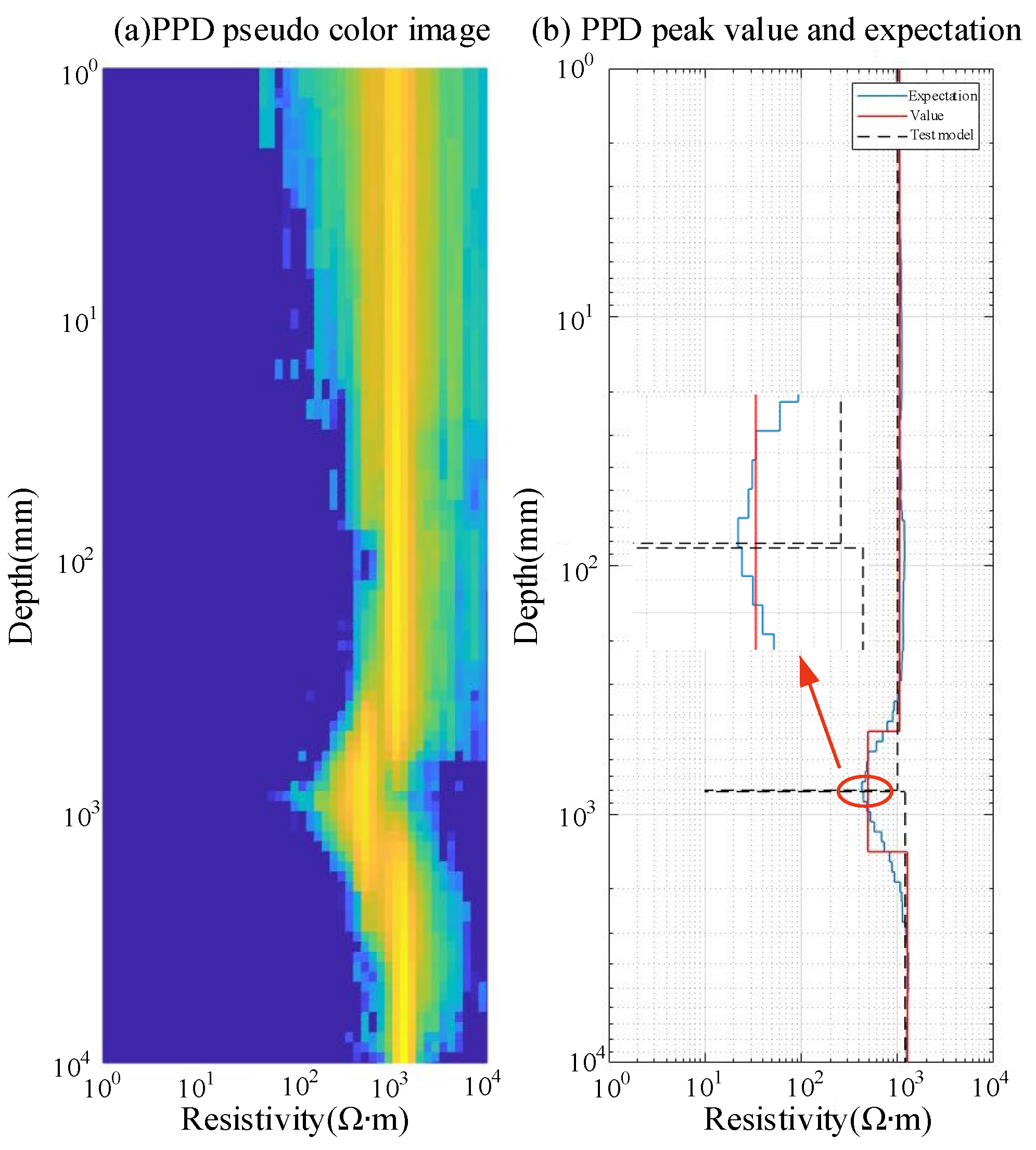
The resulting parameter identification results are shown in Figure 6.
In Figure 6, PDD represents the posterior probability density P(m|d). From (b), it can be seen that the grounding grid’s position range is [739.072, 811.131] mm, while the forward model’s range is [800, 812] mm. In actual working conditions, the depth of the grounding grid is calculated based on the side of the grounding grid closest to the ground. However, since the Bayesian parameter identification results provide a general range for parameter identification, the measurement error is calculated using the boundary values of both intervals. Specifically, the parameter identification range is set as [h_1, h_2], and the forward model’s range average is [h_3, h_4]. The MSE_h (Mean Squared Error) calculation formula is given by
M S E _ h = ( h _ 1 h _ 3 h _ 3 + h _ 2 h _ 4 h _ 4 ) / 2 × 100 %
Using Equation (33), the error is found to be 3.86%, with a central distance of approximately 3.1 cm. The obtained result meets the measurement requirements.

4.2. Parameter Identification Results for Grounding Grid Depth Variation

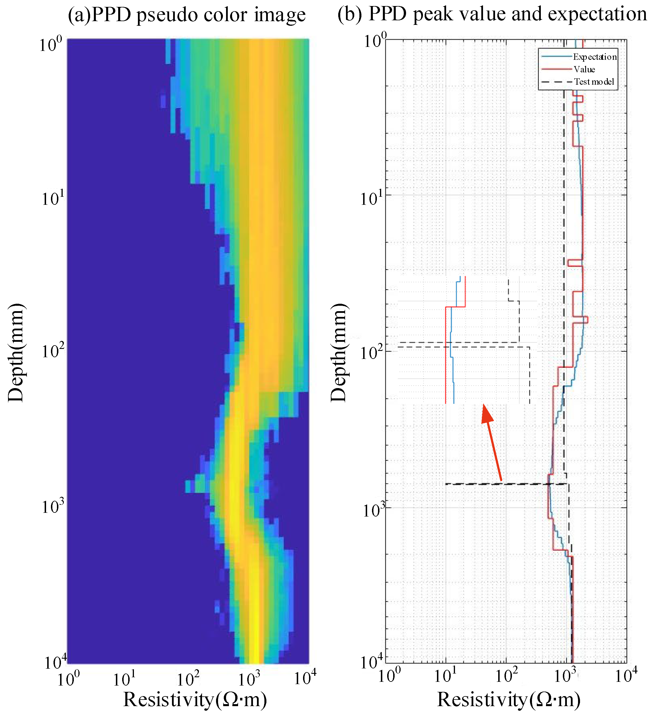
As shown in Figure 7, electromagnetic parameter identification for the variation in grounding grid depth is conducted, with the input model parameters shown in Table 2. The obtained depth information for the grounding grid is [673.415, 739.072] mm. Using Equation (33), the MSE_h error is calculated to be 3.80%, with a central distance of approximately 2.44 cm. The obtained result meets the measurement requirements.
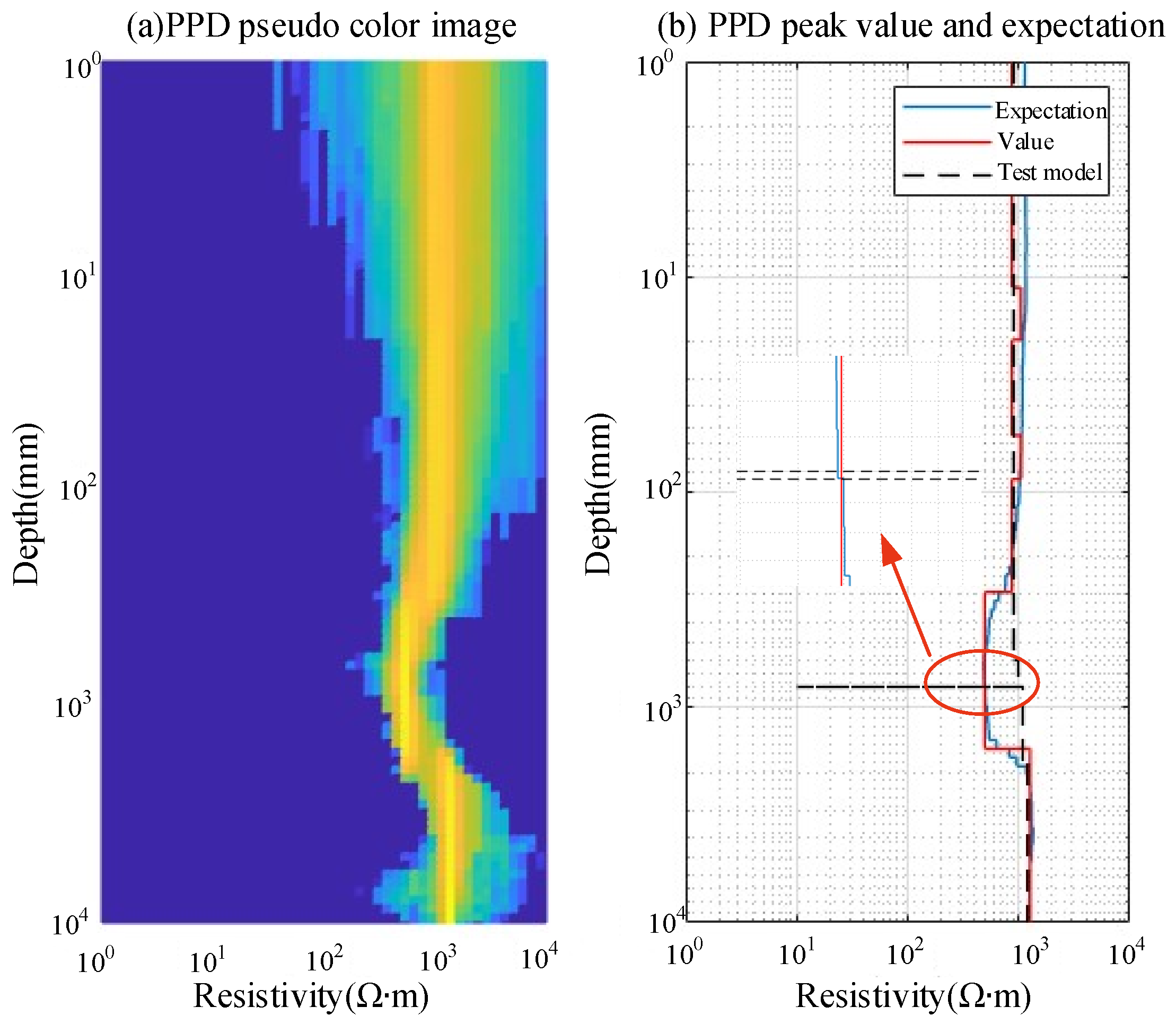
As shown in Figure 8, the parameter identification structure indicates that the depth information is [739.05, 811.131] mm. Using Equation (33), the MSE_h error is calculated to be 3.88%, with a central distance of approximately 3.09 cm. The obtained result meets the measurement requirements.
The parameter identification results for grounding grid depths of 0.7 m and 0.8 m demonstrate that, under slight noise conditions, the error values obtained using Equation (33) are all within 10%, and the midpoint distance between the most likely interval for representing the grounding grid position, identified by the parameter identification, and the midpoint of the interval set in the forward model is also less than 10 cm.

5. Experimental Validation

5.1. Experimental Process

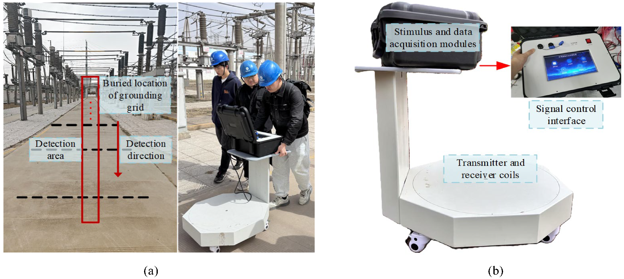
This study presents a signal acquisition study of a substation in a certain region using a pulsed eddy current device. The grounding detection device adopts a concentric integrated design of an emitting coil and a receiving coil. The number of turns of the emitting coil is 50, with a single-turn diameter of 2 mm, and the diameter of the coil frame is 600 mm. The number of turns of the receiving coil is 1400, with a diameter of 0.5 mm. The excitation current of the emitting coil is a 20 A pulse square wave with a frequency of 25 Hz. The sampling rate of the receiving coil is 125 MHz, and the sampling accuracy is 14 bits. The acquisition method is point-based, meaning measurements are taken at intervals of 0.5 m. Each measurement point should capture data for at least 100 cycles. The field measurement setup is shown in Figure 9a. In this experiment, the excitation current is set to 30 A, utilizing a bipolar pulsed current with a frequency of 25 Hz. The coil radius is 0.3 m, and the turn-off time is approximately 10μs. A schematic diagram of the detection device is shown in Figure 9b.
The sampling rate of the receiving system is 1 MHz, with a gain factor of 100 times and 300 turns for the receiving coil. According to the Chinese Standard. Electrical Installation Engineering Grounding Device Construction and Acceptance Specification GB 50169-2016, Beijing: China Electricity Council, the soil resistivity and the burial depth of the grounding device should meet the requirements specified in the table below to ensure the grounding resistance design meets the necessary standards.
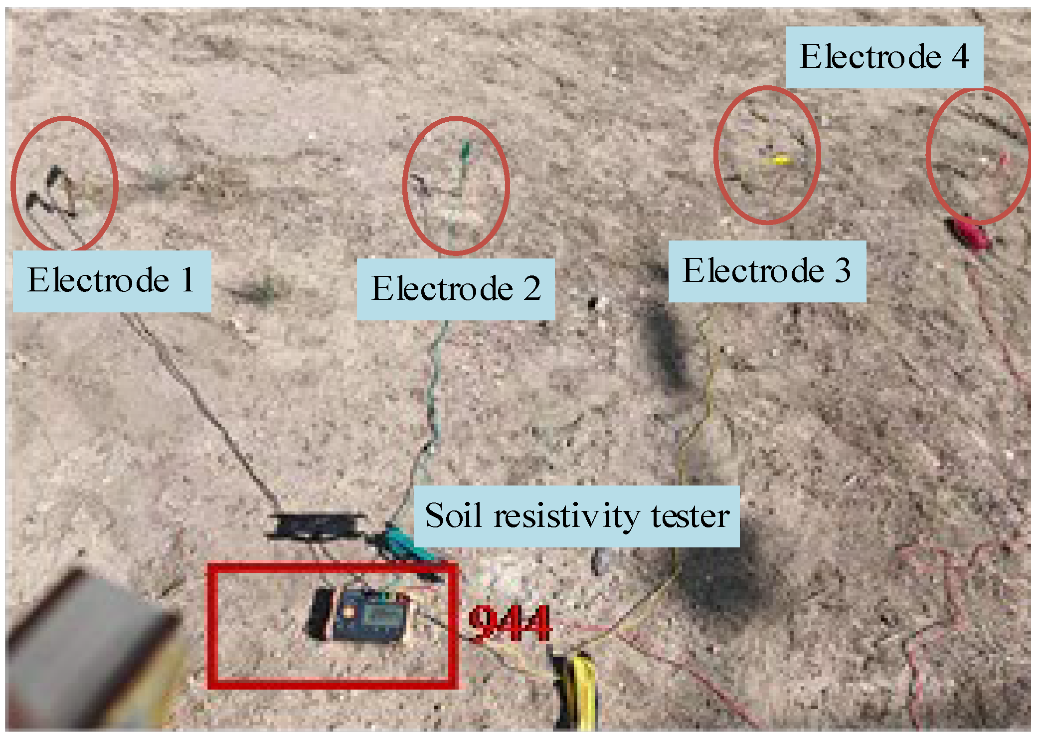
According to Table 3, it can be observed that when measuring the surface soil resistivity, the variation within a certain depth range is relatively small. Therefore, the measured resistivity can be used as a reference resistivity for the design of the substation grounding system. If the soil resistivity is known, the burial depth range of the grounding grid can be preliminarily estimated and used as prior information for the grounding grid parameter identification calculations. To improve the accuracy of the experiment, prior to its commencement, a four-electrode method was used with a soil resistivity analyzer to measure the soil resistivity near the substation. The measurement results are shown in Figure 10.
During the testing process, the distance between each electrode was set to 1 m. The measured soil resistivity value was 944 Ω·m. According to Table 3, the reasonable burial depth range for the grounding grid should be no less than 0.5 m. This result can serve as prior information for the subsequent grounding grid parameter identification calculations.

5.2. Parameter Identification Results

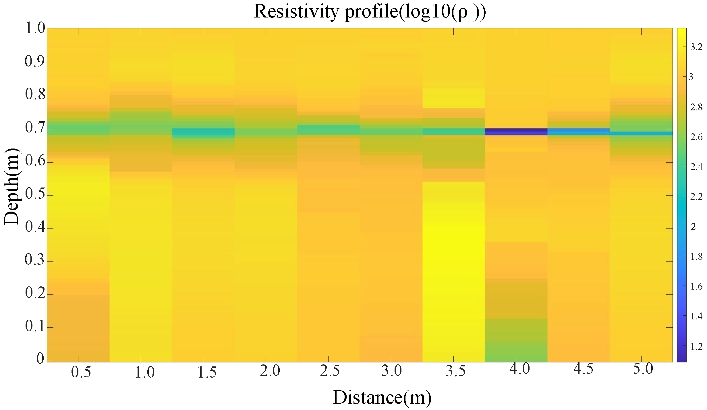
The variable dimensional Bayesian parameter identification algorithm is employed to calculate the posterior resistivity probability density distribution, which satisfies the data collected and processed through signal processing, as well as the prior information obtained in the previous section. The parameter settings for Bayesian parameter identification are consistent with those in Table 2, with a maximum sampling iteration of one million times and a burn-in sampling of ten thousand times. The model depth range is set between 3 and 10 layers. A total of 10 measurement points are located along the measurement line, with a spacing of 2 m between each point. The multi-point parameter identification results are shown in Figure 11.
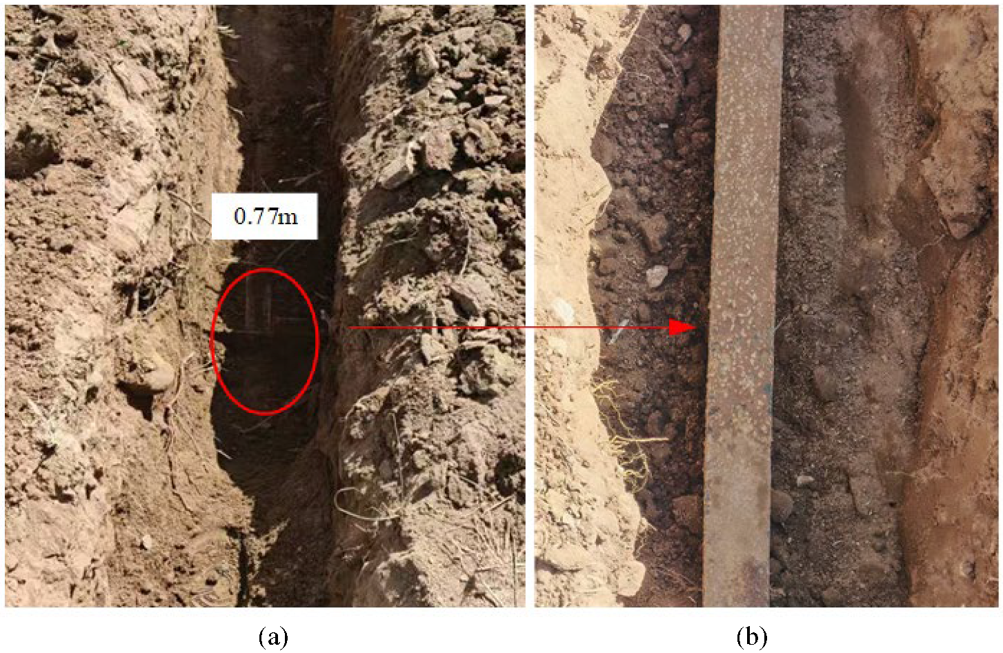
In Figure 11, the horizontal axis represents the distance between the 10 measurement points, while the vertical axis indicates the depth information at different points. The color information represents the resistivity of each layer. As shown in the figure, the signal at almost every measurement point shows a variation at the 0.7 m depth layer, indicating the presence of a grounding grid at this depth. The estimated burial depth of the grid is approximately 0.7 m. Excavation verification was then conducted, as shown in Figure 12, where the measured grounding grid burial depth was approximately 0.77 m. The difference between the measured depth and the parameter identification result is 7 cm, with an error of about 9.1%. This demonstrates that the pulsed electromagnetic signal processing and analysis method proposed for substation grounding grid detection in this paper has achieved satisfactory results in detecting the grounding grid depth.
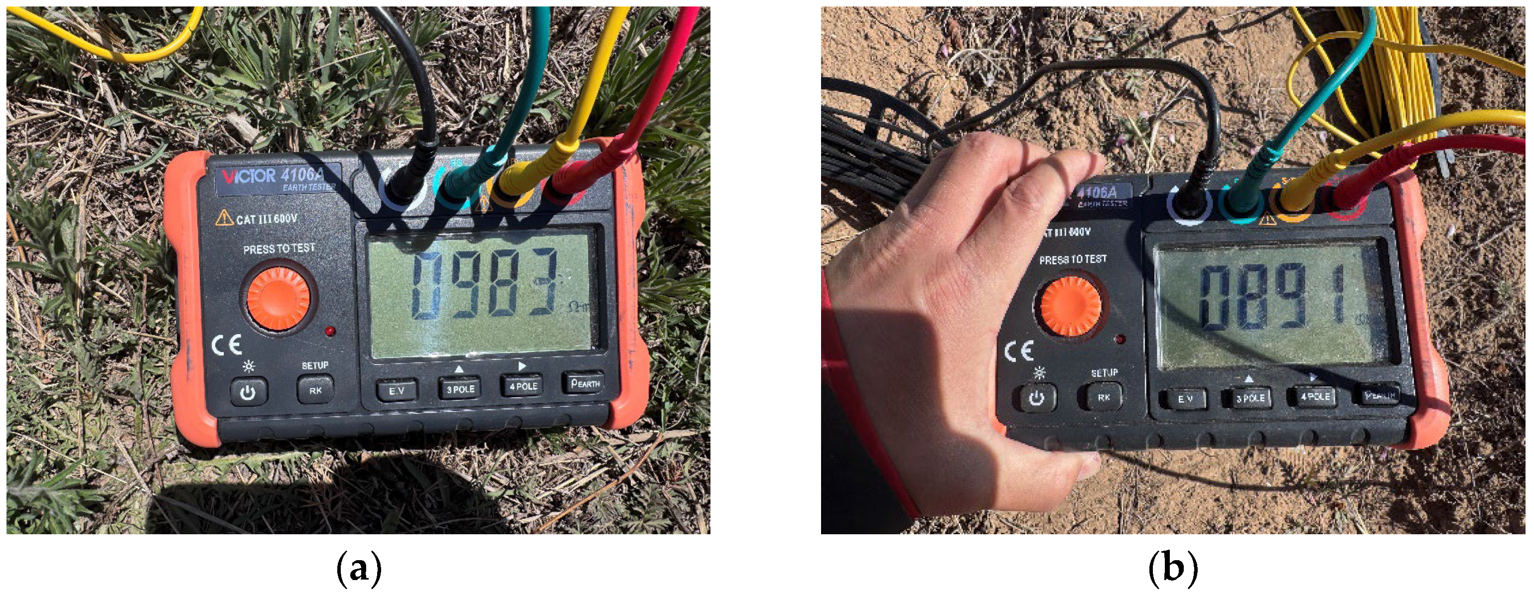
Through the multiple measurement results of Table 4, it can be seen that the average error between the real results and the parameter identification results is about 7.82%. The parameter identification results proposed in this paper are in good agreement with the actual situation under multiple measurements. The standard deviation of the error of multiple measurement results is 0.0119, which proves the stability of multiple measurement results. In addition, tests were conducted at two additional substations. For soil resistivity measurement, the protocol of the “four-electrode soil resistivity analyzer” described above was followed, with the results presented in Figure 13. The measured soil resistivities of the two substations were 983 Ω·m and 891 Ω·m, respectively; meanwhile, 10 measurement points were arranged in each newly added substation, and consistent pulsed eddy current data acquisition and parameter identification procedures from the original text were adopted to complete the measurement and identification of the grounding grid burial depth. The corresponding results are shown in Table 5 and Table 6, respectively.
Derived from the data in Table 5 and Table 6, the average values of the identification results for the grounding grid burial depth parameters of the other two substations are 8.58% and 8.69%, respectively. This further demonstrates the reliability and accuracy of the pulsed eddy current parameter identification method based on RJMCMC proposed in this paper under different soil environments.

6. Conclusions

This study addresses the issue of local optima that often arise in parameter identification during substation grounding grid detection using the pulsed eddy current method. A grounding grid burial depth parameter identification method based on variable dimensional Bayesian inference is proposed. First, a numerical forward model of the electromagnetic response of the grounding grid based on magnetic dipoles is derived and subsequently validated. The results demonstrate that the model effectively characterizes the electromagnetic response features of the grounding grid. Second, the RJMCMC method is introduced to enable adaptive adjustment of the model’s dimensionality, thereby enhancing the global search capability for parameter identification. A ω-c dual-factor adjustment mechanism is incorporated to improve the resistivity resolution, and a dynamic step size control strategy is adopted to increase computational efficiency. Additionally, a convergence criterion based on uncertainty assessment is introduced, significantly reducing the number of sampling iterations and accelerating the Bayesian parameter identification process. The proposed method is validated using the forward model, and the results show that, under 5% noise interference, the depth information obtained through parameter identification deviates by less than 10 cm from the model depth, with an error of less than 10%. Finally, experimental verification is carried out at a substation in Inner Mongolia, China. The identified grounding grid burial depth is 0.7 m, with a deviation of 9.1% from the actual value, demonstrating the practicality of the proposed parameter identification method.

Author Contributions

Conceptualization, X.K. and Z.L.; methodology, X.K. and J.W.; software, J.H. and S.X.; validation, X.K., Z.L. and J.W.; formal analysis, X.K. and S.X.; investigation, Y.Z. and Z.Z.; resources, Z.Z.; data curation, X.K. and Y.Z.; writing—original draft preparation, X.K.; writing—review and editing, Z.Z.; visualization, J.H. and Z.Z.; supervision, Y.Z.; project administration, S.X.; funding acquisition, J.H. All authors have read and agreed to the published version of the manuscript.

Funding

This research was funded by Inner Mongolia Power (Group) Co., Ltd. Science and Technology Project, Grant No. nmgdlkjxm20240403.

Data Availability Statement

The data used in the analysis presented in the paper will be made available, subject to the approval of the correspondence author.

Conflicts of Interest

The authors declare that this study received funding from Baotou Power Supply Bureau of Inner Mongolia Power Grid Co., Ltd. All authors declare that the research was conducted in the absence of any commercial or financial relationships that could be construed as a potential conflict of interest. The funder was involved in the study design, collection, analysis, interpretation of data, the writing of this article, or the decision to submit it for publication.

References

  1. Zhang, B.; He, J.L.; Zeng, R. State of art and prospect of grounding technology in power system. High Volt. Eng. 2015, 41, 2569–2582. [Google Scholar] [CrossRef]
  2. Xu, X.Y. Research on Fault Diagnosis for Grounding Grid in Substation Based on Tikhonov Regularized Principle. Master’s Thesis, Chongqing University, Chongqing, China, 2017. [Google Scholar]
  3. Wang, Y.; Zhang, W.X.; Wang, C.; Li, Z.; Luo, B.; Yan, F.; Zhang, H. Study on numerical simulation of electromagnetic response of intelligent substation grounding grid based on multi-grid partitioning technology. Electr. Meas. Instrum. 2024, 61, 97–103. [Google Scholar]
  4. Peng, L.S.; Sun, H.Y.; Li, S.S.; Wang, S.; Huang, S.L. Mix-frequency SH guided wave corrosion defects detection method for high voltage transmission tower grounding electrode. Trans. China Electrotechn. Soc. 2025, 40, 376–386. [Google Scholar] [CrossRef]
  5. Xu, Z.; Liao, X.; Liu, L.; Fu, N.; Fu, Z. Research on Small-Loop Transient Electromagnetic Method Forward and Nonlinear Optimization Inversion Method. IEEE Trans. Geosci. Remote Sens. 2023, 61, 1–13. [Google Scholar] [CrossRef]
  6. Chen, X.G.; Lei, Y.Z. Analytical expressions of induced coil voltages generated by pulsed eddy currents for metal pipe testing. Proc. CSEE 2012, 32, 176–182. [Google Scholar] [CrossRef]
  7. Yu, C.; Fu, Z.; Wu, G.; Zhou, L.; Zhu, X.; Bao, M. Configuration Detection of Substation Grounding Grid Using Transient Electromagnetic Method. IEEE Trans. Ind. Electron. 2017, 64, 6475–6483. [Google Scholar] [CrossRef]
  8. She, S. Thickness measurement and surface-defect detection for metal plate using pulsed eddy current testing and optimized Res2Net network. IEEE Trans. Instrum. Meas. 2024, 73, 1–13. [Google Scholar] [CrossRef]
  9. Fang, J. Modelling and experimental study on pipeline defect characterisations using a pulsed eddy current measurement. Nondestruct. Test. Eval. 2024, 40, 4024–4045. [Google Scholar] [CrossRef]
  10. Zeng, Z.W.; Guo, Z.; Gan, F.; Zuo, Y.; Tian, X.; Wang, X.; Lin, Z.; Zhu, W.; Wang, X.; Wang, J. Array coil design and experimental verification for separation of tower grounding pulsed eddy current excitation and response magnetic field signals. Energies 2025, 18, 364. [Google Scholar] [CrossRef]
  11. Jiang, Y.; Xu, Z.; Wu, P.; Huang, L.; Meng, C. A Time-Domain Calibration Method for Transient EM Field Sensors. Measurement 2021, 168, 108368. [Google Scholar] [CrossRef]
  12. Wang, H.; Fu, Z.; Wang, Y.; Tai, H.-M.; Chen, W. On-Site Calibration of Air-Coil Sensor for Transient Electromagnetic Exploration. Geophys. Prospect. 2019, 67, 1595–1610. [Google Scholar] [CrossRef]
  13. Guan, W.J.; Chen, Y.; Wu, W.; Zheng, Q.; Yan, L.; Lu, Y. Fault detection method of substation ground grid based on transient electromagnetic method. In International Conference of Electrical, Electronic and Networked Energy Systems; Springer Nature: Singapore, 2024. [Google Scholar] [CrossRef]
  14. Chen, W.Y.; Xue, G.; Lei, K.; Song, W. Transient electromagnetic smoke ring due to a grounded-wire source. Pure Appl. Geophys. 2023, 180, 2157–2168. [Google Scholar] [CrossRef]
  15. Smiarowski, A.; Hodges, G. Transient electromagnetic smoke rings in a half-space during active transmitter excitation. Geophysics 2021, 86, E199–E208. [Google Scholar] [CrossRef]
  16. Pasion, L.R. Detecting Unexploded Ordnance with Time Domain Electromagnetic Induction. Ph.D. Thesis, University of British Columbia, Vancouver, BC, Canada, 1999. [Google Scholar] [CrossRef]
  17. Wang, L.; Zhang, S.; Chen, S.; Jiang, H. Fast localization of underground targets by magnetic gradient tensor and Gaussian-Newton algorithm with a portable transient electromagnetic system. IEEE Access 2021, 9, 148469–148478. [Google Scholar] [CrossRef]
  18. Wang, H.; Chen, S.; Zhang, S.; Yuan, Z.; Zhang, H.; Fang, D.; Zhu, J. A high-performance portable transient electromagnetic sensor for unexploded ordnance detection. Sensors 2017, 17, 2651. [Google Scholar] [CrossRef]
  19. Chen, S.; Zhang, S.; Zhu, J.; Luan, X. Accurate measurement of characteristic response for unexploded ordnance with transient electromagnetic system. IEEE Trans. Instrum. Meas. 2019, 69, 1728–1736. [Google Scholar] [CrossRef]
  20. Chen, S.; Zhang, S.; Luan, X.; Liu, Z. Improved differential evolution algorithm for multi-target response inversion detected by a portable transient electromagnetic sensor. IEEE Access 2020, 8, 208107–208119. [Google Scholar] [CrossRef]
  21. Šimić, M.; Ambruš, D.; Bilas, V. Rapid object depth estimation from position-referenced EMI data using machine learning. IEEE Sens. J. 2023, 23, 4285–4293. [Google Scholar] [CrossRef]
  22. Šimić, M. Machine Learning Based OBJECT classification from Pulse Induction Metal Detector Data. Ph.D. Dissertation, University of Zagreb, Zagreb, Croatia, 2024. [Google Scholar]
  23. Li, S.; Zhang, X.; Xing, K.; Zheng, Y. Fast inversion of subsurface target electromagnetic induction response with deep learning. IEEE Geosci. Remote Sens. Lett. 2022, 19, 1–5. [Google Scholar] [CrossRef]
  24. Chen, J.; Yan, F.; Sun, Y.; Zhang, Y. Applicability of transient electromagnetic fast forward modeling algorithm with small loop. Prog. Electromagn. Res. M 2020, 98, 159–169. [Google Scholar] [CrossRef]
  25. Guptasarma, D. New digital linear filters for Hankel J0 and J1 transforms. Geophys. Prospect. 2010, 45, 745–762. [Google Scholar] [CrossRef]
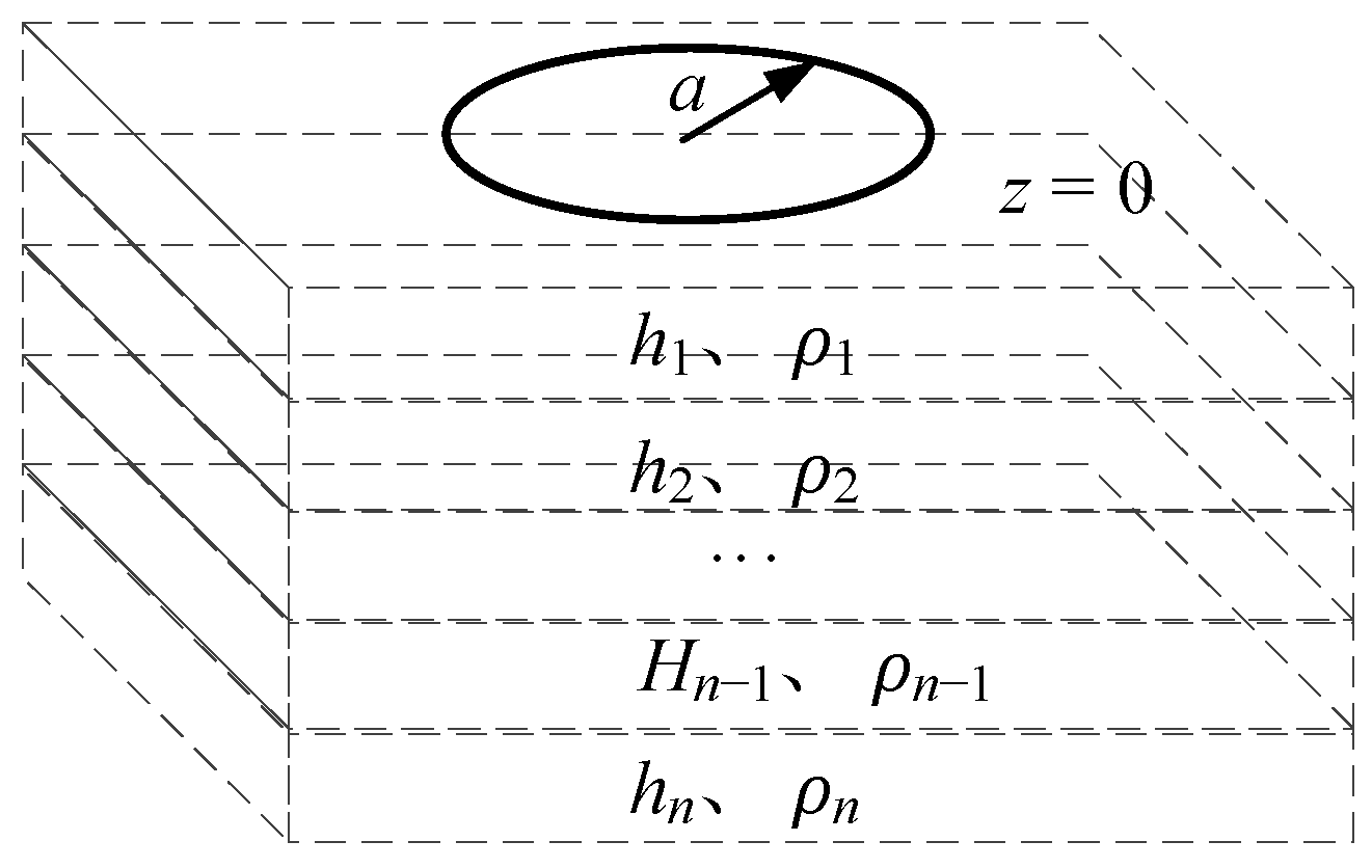
Figure 1. Schematic of the layered model.
Energies 18 04649 g001
Figure 2. H-type grounding grid electromagnetic model.
Energies 18 04649 g002
Figure 3. Pulse eddy current forward signal of H-type grounding grid.
Energies 18 04649 g003
Figure 4. Schematic of four possible states of the new model generated by RJMCMC sampling.
Energies 18 04649 g004
Figure 5. Flowchart for parameter identification of substation grounding grid electromagnetic data.
Energies 18 04649 g005
Figure 6. Dimensional Bayesian parameter identification results for H-type grounding grid model.
Energies 18 04649 g006
Figure 7. Dimensional Bayesian parameter identification results for grounding grid with depth of 0.7 m.
Energies 18 04649 g007
Figure 8. Dimensional Bayesian parameter identification results for grounding grid with depth of 0.8 m.
Energies 18 04649 g008
Figure 9. Field signal acquisition and detection device. (a) On-site detection schematic diagram. (b) Grounding detection device.
Energies 18 04649 g009
Figure 10. Soil resistivity testing method and results.
Energies 18 04649 g010
Figure 11. Multi-point Bayesian parameter identification results.
Energies 18 04649 g011
Figure 12. Excavation verification results. (a) Field excavation diagram. (b) Localized enlarged view.
Energies 18 04649 g012
Figure 13. Substation soil resistivity test results. (a) The first substation resistivity measurement result. (b) Second substation resistivity measurement result.
Energies 18 04649 g013
Table 1. H-type model parameters.
ResistivityUnit (Ω∙m)ThicknessUnit (m)
ρ1900h10.8
ρ21/(5.6 × 106)h20.012
ρ31000h3
Table 2. Parameter settings for dimensional Bayesian parameter identification.
ParametersValues
Minimum Number of Model Layer Interfaces3
Maximum Number of Model Layer Interfaces10
Number of Burn-in Phases10,000
Total Number of Samples1,000,000
Number of Markov Chains1
Resistivity Update Step Size σchange4
Layer Interface Perturbation Step Size σmove10
New Layer Generation Step Size σbirth4
Table 3. Soil resistivity and burial depth and maximum length of grounding devices.
ρ (Ω∙m)100 < ρ ≤ 500500 < ρ ≤ 10001000 < ρ ≤ 2000>2000
Depth (m)≥0.6≥0.5≥0.5≥0.3
Maximum Length (m)406080100
Table 4. Measurement results of 11 measuring points on site.
Measuring PointMeasured Value z (m)True value zreal (m)Error Err
10.820.767.89%
20.730.786.41%
30.830.777.79%
40.690.758.00%
50.870.7910.13%
60.700.767.89%
70.850.788.97%
80.720.776.49%
90.790.746.76%
100.710.788.97%
110.800.756.67%
Table 5. Measurement results of 10 measuring points on first substation.
Measuring PointMeasured Value z (m)True Value zreal (m)Error Err
11.060.988.16%
20.931.017.92%
31.011.119.01%
41.050.969.38%
50.941.027.84%
61.040.968.33%
71.060.979.28%
80.951.037.77%
90.941.049.62%
100.971.068.49%
Table 6. Measurement results of 10 measuring points on second substation.
Measuring PointMeasured Value z (m)True Value zreal (m)Error Err
11.291.189.32%
21.311.1910.08%
31.111.218.26%
41.121.206.67%
51.321.2010.00%
61.271.169.48%
71.091.187.63%
81.121.238.95%
91.111.218.26%
101.101.197.56%
Disclaimer/Publisher’s Note: The statements, opinions and data contained in all publications are solely those of the individual author(s) and contributor(s) and not of MDPI and/or the editor(s). MDPI and/or the editor(s) disclaim responsibility for any injury to people or property resulting from any ideas, methods, instructions or products referred to in the content.