Article

Multi-Objective Optimization of 12-Pole Radial Active Magnetic Bearings with Preference-Based MOEA/D Algorithm

School of Electrical and Information Engineering, Tianjin University, Tianjin 300072, China
*
Author to whom correspondence should be addressed.
Energies 2025, 18(16), 4299; https://doi.org/10.3390/en18164299
Submission received: 16 July 2025 / Revised: 10 August 2025 / Accepted: 10 August 2025 / Published: 12 August 2025
(This article belongs to the Section F: Electrical Engineering)

Abstract

In this paper, the multi-objective optimization of the 12-pole radial active magnetic bearing (RAMB) is investigated. In the optimization of the RAMB, the decision-maker is more interested in the Pareto-optimal solutions in a certain region. This paper proposes a decomposition-based and preference-based multi-objective evolutionary algorithm (MOEA/D-Pref). The proposed MOEA/D-Pref not only allows the number of Pareto-optimal solutions to be more concentrated in the region of interest but also preserves solutions in other regions. These preserved solutions enable decision-makers to observe a more complete Pareto front, thus gaining more comprehensive insights. In this paper, a mathematical model of the 12-pole RAMB is established, and, with the help of this model and the proposed algorithm, the optimal design of the 12-pole RAMB is completed. The difference between the current stiffness coefficients of the optimized RAMB, calculated by the proposed algorithm and by the finite element method, is 2.3%. The difference between the displacement stiffness coefficient of the optimized RAMB as calculated by the proposed algorithm and by the finite element method is 3.9%. These differences, being less than 4%, are relatively low and verify the reliability of the mathematical model established.

1. Introduction

An active magnetic bearing (AMB) has the advantages of not requiring lubrication, lower noise, active control and a high power density; it has a wide range of applications in the industrial field, such as flywheel energy storage, motorized spindles, centrifugal compressors and so on [1,2,3,4,5]. Their contactless operation, adaptive stiffness and active control capabilities make them superior to traditional bearings in extreme conditions. The radial active magnetic bearing (RAMB) is a type of AMB that is primarily responsible for providing an electromagnetic force along the radial direction perpendicular to the rotational axis.
The performance characteristics of radial active magnetic bearings (RAMBs) are fundamentally governed by their structural parameters, necessitating the systematic optimization of these design variables. Single-objective optimization techniques have been employed to enhance the performance of RAMBs [6,7]. However, multi-objective optimization methods are better suited to RAMB design due to their ability to simultaneously optimize conflicting performance aspects through Pareto-optimal solutions. They provide balanced trade-offs while considering electromagnetic, thermal and dynamic constraints, enabling more comprehensive and practical designs for complex AMB systems [8,9,10,11,12,13,14].
Several algorithms have been developed to solve these multi-objective optimization problems, such as NSGA-II [15], MOEA/D [16], KnEA [17], IWOA [18] and NSGA-III [19]. Although these algorithms have distinct characteristics, they share a common ultimate objective: to generate a well-distributed Pareto-optimal solution set. In the practical application of multi-objective optimization, decision-makers may be more interested in the Pareto-optimal solutions in a particular region. This particular region is the region of interest for the decision-maker. The multi-objective optimization of RAMBs has this characteristic. In the optimization of RAMBs, once the load capacity exceeds a well-defined target value, pursuing designs with a greater load capacity becomes meaningless. This is because such pursuit would inevitably compromise other critical performance aspects. The optimal solution chosen by the decision-maker from the Pareto-optimal solution set tends to be in the vicinity of the target value in terms of the load capacity. The region of interest is the region around the target load capacity value. Preference-based multi-objective optimization methods are particularly well suited to solving this type of problem, and they can enable the distribution of Pareto-optimal solutions to meet the preferences of decision-makers. Some preference-based multi-objective optimization algorithms have been proposed. A g-dominance method based on decision-makers’ given reference points is proposed in [20]. The position of the reference point has a significant impact on the algorithm with g-dominance. When the reference point is set near the Pareto front, the algorithm may not converge. In [21], an r-dominance method based on decision-makers’ given reference points is proposed. Compared with g-dominance, the r-dominance method is less affected by preference points, but r-dominance can only guarantee weak Pareto dominance optimality. An angle-dominated NSGA-II (AD-NSGA-II) based on the angle relationship between individuals is proposed in [22]. This algorithm redefines the dominance relationship and aggregation distance between individuals, giving priority to retaining individuals that are close to the preference point. Reference [23] proposes the reference point-based multi-objective optimization through decomposition algorithm (R-MOEA/D), which introduces a decomposition method to convert the position information of the reference point into a set of weight vectors carrying preference information. Although these preference-based multi-objective optimization methods achieve the desired preference effects on test functions, the method by which they introduce preference information is not suitable for the optimization of RAMBs based on the load capacity target value preference. Decision-makers cannot determine reference points based solely on carrying capacity target values. Correctly introducing preference information is important in achieving the preference effects desired by decision-makers. In order to achieve the appropriate expression of preference information, a decomposition-based and preference-based multi-objective evolutionary algorithm (MOEA/D-Pref) for the optimization of RAMBs is proposed. The Pareto-optimal solution set obtained by MOEA/D-Pref is denser in the regions closer to the target value and sparser in the regions farther away from the target value. Thus, MOEA/D-Pref not only allows the number of Pareto-optimal solutions to be more concentrated in the region of interest but also preserves solutions in other regions. These preserved solutions enable decision-makers to observe the complete shape of the Pareto front, thereby gaining more comprehensive insights.
This paper aims to achieve an optimized design for a 12-pole RAMB. Firstly, the mathematical model of the 12-pole RAMB is derived via the equivalent magnetic circuit method. The optimization objective function and parameters are determined with the help of the model. Secondly, MOEA/D is used to calculate the Pareto-optimal solution set for the multi-objective optimization of the 12-pole RAMB. Thirdly, MOEA/D-Pref is introduced, and it is used to calculate the Pareto-optimal solution set for the multi-objective optimization of the 12-pole RAMB. Finally, the optimal design of the 12-pole RAMB is obtained by using the proposed MOEA/D-Pref.

2. Structure and Mathematical Modeling of the 12-Pole RAMB

2.1. Structure of the 12-Pole RAMB

According to the flux path, RAMBs can be categorized into two types: homopolar RAMBs and heteropolar RAMBs. In homopolar RAMBs, the magnetic poles are arranged axially, meaning that the flux path flows along the axial direction. In heteropolar RAMBs, the magnetic poles are arranged radially, meaning that the flux path flows along the radial direction. According to the magnetic pole distribution, heteropolar RAMBs can be further divided into the coupled type and decoupled type. The topology of the coupled type has the magnetic poles distributed according to the order of NSNS, while the decoupled topology has the poles distributed in the order of NSSN. The heteropolar decoupled structure, characterized by high magnetic circuit utilization and easy control, has a wider range of applications [24]. This structure serves as the research subject in this paper. These structures are shown in Figure 1. The direction of the arrows in the Figure 1 represents the direction of the magnetic field.
The number of poles in a RAMB is generally determined according to the size of the shaft diameter [25]. The number of poles of the RAMB used to support the rotor of a high-speed motor, as studied in this paper, is selected to be 8, 12 and 16. RAMBs with fewer poles perform better in terms of load capacity, but RAMBs with 8 poles are not as beneficial as RAMBs with 12 and 16 poles in terms of control accuracy. Moreover, RAMBs with 12 poles have a smaller stator yoke thickness and higher utilization of the magnetic circuit. Therefore, in this paper, a 12-pole RAMB of the heteropolar decoupling type is chosen as the research object.

2.2. Mathematical Modeling of the 12-Pole RAMB

AMBs achieve stable rotor levitation by generating controllable electromagnetic forces. This paper derives the mathematical expression of these electromagnetic forces and establishes their mathematical model. Based on this model, this paper conducts structural parameter design and the optimization of RAMBs. In order to reduce the difficulty in establishing the mathematical model, the following assumptions are made during modeling: (1) the permeability of both the stator and rotor iron cores is assumed to be infinite; (2) magnetic leakage and hysteresis effects are neglected; (3) the magnetic field is uniformly distributed in both the iron cores and air gaps; (4) the magnetic saturation characteristics of ferromagnetic materials are neglected; (5) eddy currents in the iron cores are neglected.
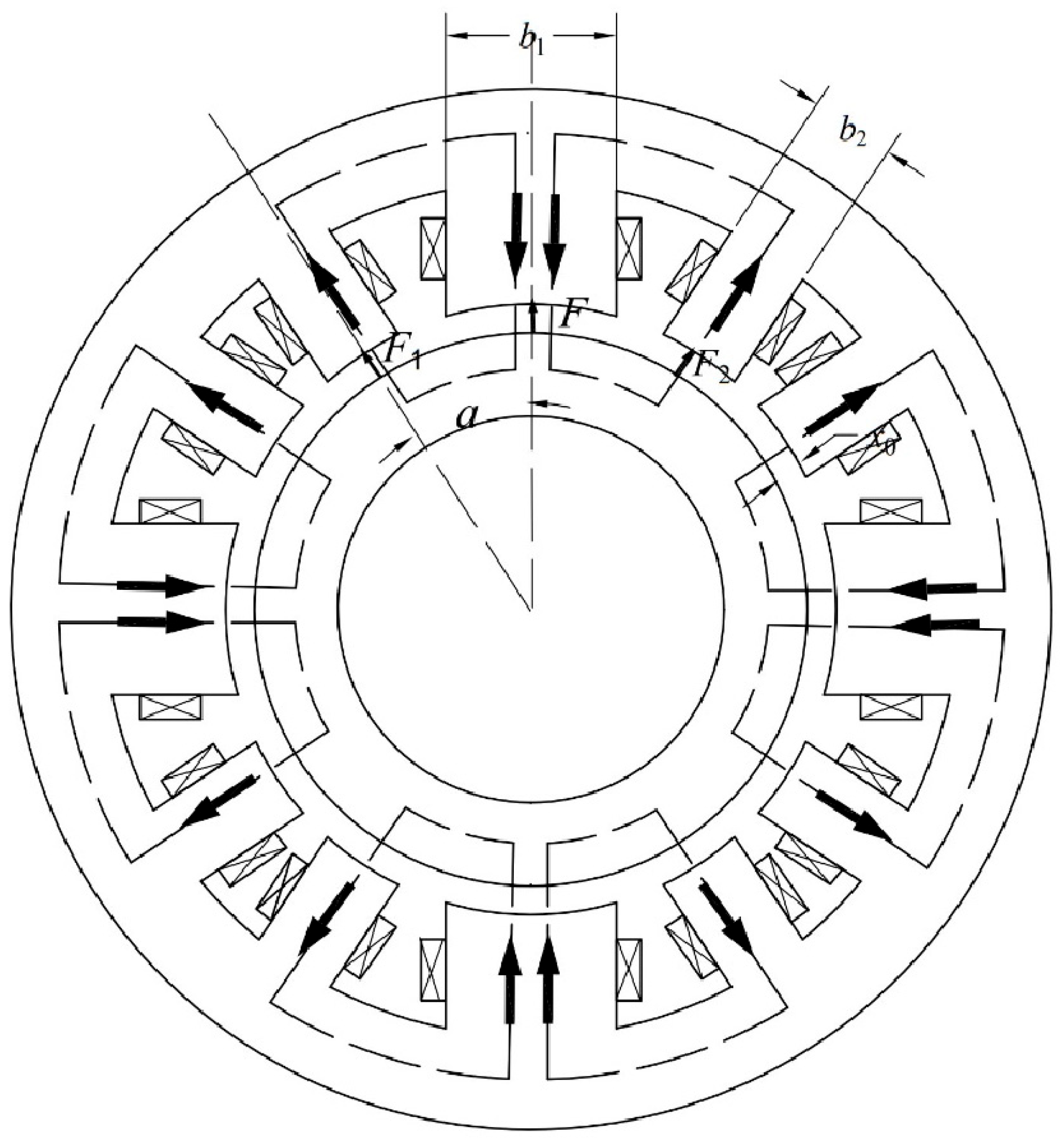
The mathematical modeling of the RAMB is achieved via the equivalent magnetic circuit method. Figure 2 illustrates the structure and magnetic circuit of a 12-pole heteropolar decoupled RAMB. The direction of the arrows in the Figure 2 represents the direction of the magnetic field. The twelve magnetic poles can be divided into four “pole units” according to the magnetic circuit, and one “pole unit” consists of two secondary magnetic poles and one primary magnetic pole. Neglecting magnetic leakage, the magnetic flux on the main magnetic pole enters into the two secondary magnetic poles. When the relationship between the pole width of the primary pole and the pole width of the secondary pole is in accordance with Equation (1), the flux density of the air gap with these primary poles and the flux density under the secondary poles are approximately equal.
b 1 = 2 b 2
where b1 is the primary pole width and b2 is the secondary pole width.
Based on the assumptions made in the previous section, the magnetic flux density in the air gap based on the Ampere critical theorem can be expressed as
B = μ 0 ( N 1 + N 2 ) i 0 2 x 0
where N1 is the coil turn count on the primary poles, N2 is the coil turn count on the secondary poles, i0 is the magnitude of the current passing through the coils on the primary and secondary poles, x0 is the length of the air gap between the stator core and the rotor core, and μ0 is the vacuum permeability.
By means of the virtual work method, the electromagnetic force imposed on the rotor by one primary pole can be expressed as
F = B 2 S 1 2 μ 0 = μ 0 ( N 1 + N 2 ) 2 i 0 2 S 1 8 x 0 2
where S1 is the cross-sectional area of the primary pole.
The electromagnetic combined force on the rotor generated by one primary pole and two secondary poles in a pole unit can be expressed as
F = F 1 + 2 F 2 cos α
where F1 is the electromagnetic force generated by a primary pole on the rotor, and F2 is the electromagnetic force generated by a secondary pole on the rotor. α is the angle between the centerlines of the primary and secondary poles.
Since the secondary pole’s magnetic area is 50% of the primary pole’s magnetic area and the electromagnetic force generated by the magnetic pole is proportional to the magnetic pole area, the electromagnetic force generated by the secondary magnetic pole on the rotor is half of the electromagnetic force generated by the primary magnetic pole. The combined force generated by one magnetic pole unit on the rotor can be further expressed as
F = μ 0 ( N 1 + N 2 ) 2 i 0 2 S 1 ( 1 + cos α ) 8 x 0 2
When the rotor is displaced from its central position by a downward displacement x due to an external disturbance, the displacement sensor detects this change and transmits a signal to the controller. Through differential control, the controller generates control voltage signals based on the sensor feedback using control algorithms. The voltage drives the coils to produce control current i, with the winding current in the upper magnetic pole unit being (i0 + i) and that in the opposing pole unit being (Ii). The combined force acting on the rotor can then be expressed as
F = μ 0 ( N 1 + N 2 ) 2 S 0 cos α 8 [ ( i 0 + i y x 0 + x cos α ) 2 ( i 0 i y x 0 x cos α ) 2 ] + μ 0 ( N 1 + N 2 ) 2 S 0 8 [ ( i 0 + i y x 0 + x ) 2 ( i 0 i y x 0 x ) 2 ]
where i0 represents the bias current and iy represents the control current.
When both the control current and rotor displacement are extremely small values, Equation (6) can be approximated by performing a Taylor series expansion at the operating point (x = 0, i = 0), while neglecting higher-order terms. The resulting linearized expression is
F = k x x + k i i k x = μ 0 S 0 ( N 1 + N 2 ) 2 i 0 2 1 + cos α 2 x 0 3 k i = μ 0 S 0 ( N 1 + N 2 ) 2 i 0 1 + cos α 2 x 0 2
where kx denotes the displacement stiffness coefficient, and ki denotes the current stiffness coefficient.
When the control current equals i0, the winding current in a magnetic pole unit reaches its maximum value of 2i0, and the magnetic flux density under its poles attains its peak value. According to the relationship between the air gap flux density and the control current, Bmax equals 2B0. Conversely, the winding current in the opposing magnetic pole unit reaches its minimum value of 0. The electromagnetic force that the RAMB can provide can be expressed as
F max = B max 2 S 0 ( 1 + cos α ) 2 μ 0 = μ 0 ( N 1 + N 2 ) 2 i 0 2 S 0 2 x 0 2 ( 1 + cos α )
where Bmax is the maximum magnetic flux density in the air gap.

3. Optimization of RAMB Using MOEA/D

3.1. Principles, Aggregation Approach and Normalization of MOEA/D

The decomposition-based multi-objective evolutionary algorithm (MOEA/D) is a widely used multi-objective optimization algorithm. It is able to decompose a set of conflicting optimization objectives into scalarized subproblems through an aggregation approach [26]. These subproblems are then simultaneously optimized by an evolutionary algorithm, resulting in a set of optimal solutions corresponding to the weight vectors.
The most commonly used aggregation approaches in MOEA/D are the weight sum method, Tchebysheff method and penalty-based boundary intersection method. The mathematical expression of the Tchebysheff approach is
min   g t e ( x | λ , z * ) = max 1 i m λ i ( f i ( x ) z i * )
where z* is the reference vector, λ is the weight vector and m is the number of optimization objectives.
Due to the fact that the range of variation between the optimization objectives is likely to have an order of magnitude difference in real industrial design, this leads to the optimal set of solutions becoming sparse in the direction of larger orders of magnitude. In order to ensure that the set of optimal solutions obtained by MOEA/D with uniformly distributed weight vectors is as homogeneous as possible, it is necessary to normalize the optimization objective functions during the optimization process. This operation can be expressed as
h i ( x ) = f i ( x ) f i _ min f i _ max f i _ min , i = 1 , 2 , , m
where fi_min is the minimum value of the i-th objective function at the current iteration, and fi_max is the maximum value of the i-th objective function at the current iteration.

3.2. Optimization Objective, Optimization Parameters, Constraints and Results

AMBs function by generating sufficient controllable electromagnetic forces to maintain stable rotor levitation while ensuring resilience against vibrations and impact loads, so the load capacity of a qualified RAMB should be able to resist the weight of the rotor and the predicted vibrations and shocks. The size of the RAMB has a close relationship with the cost, loss and critical speed. Smaller-volume RAMBs are more advantageous. The optimization objectives selected are to maximize the load capacity and minimize the volume. The load capacity and volume functions can be expressed as
S = D 3 l arcsin ( b 1 D 3 ) F m = B m 2 S ( 1 + cos α ) 2 μ 0
V = π 4 l ( D 2 2 D 1 2 + D 5 2 D 4 2 ) + 4 b 1 l ( D 4 D 3 )
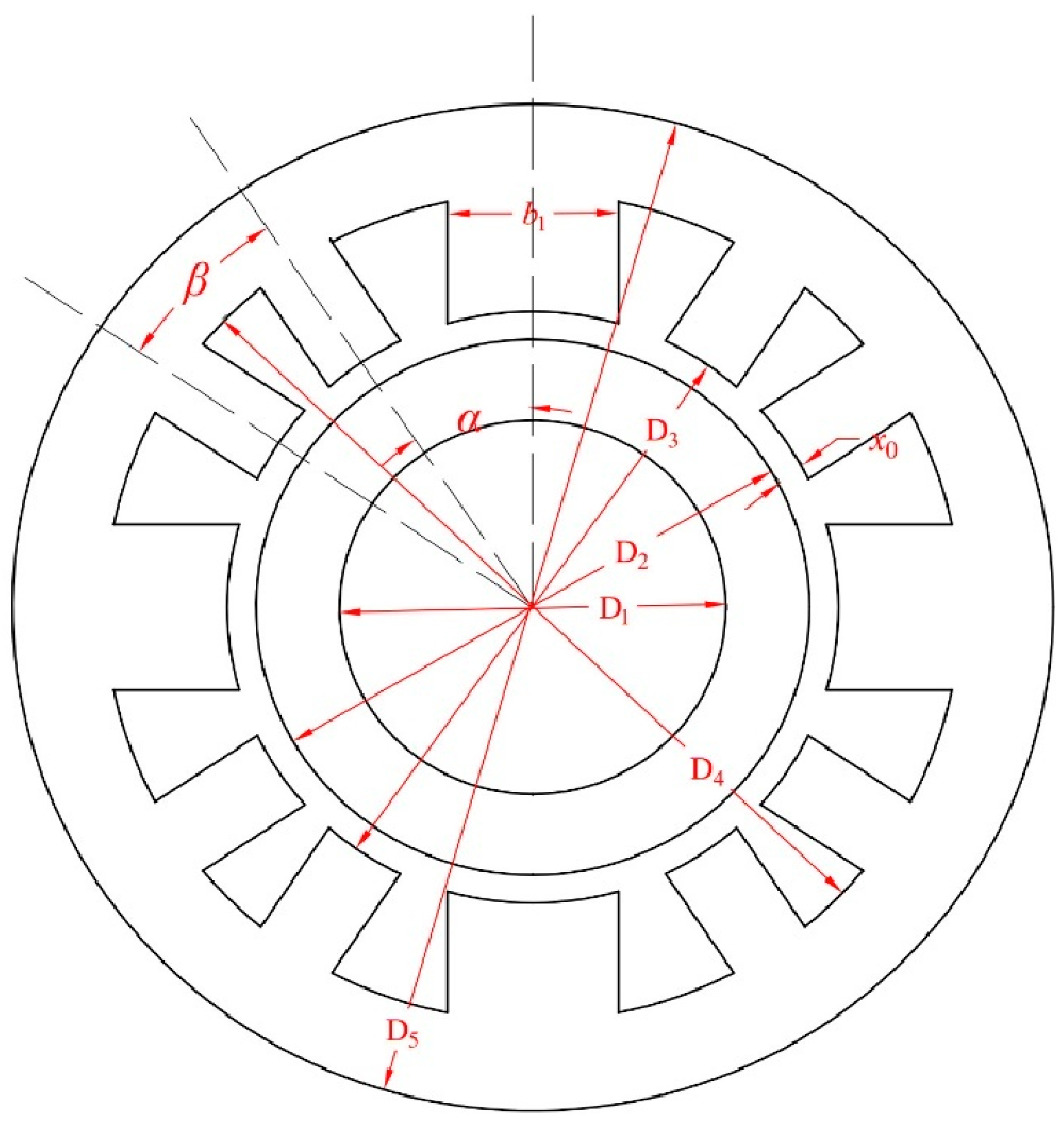
where Bm is the maximum permissible magnetic flux density in the air gap of the RAMB, l is the axial length of the radial magnetic levitation bearing, D1 is the inner diameter of the rotor, D2 is the outer diameter of the rotor, D3 is the inner diameter of the stator, D4 is the bottom diameter of the stator slot, D5 is the outer diameter of the stator, S is the area of the primary pole, α is the angle between the centerlines of the primary and secondary poles, and b1 is the primary pole width.
The 12-pole RAMB structure with structural parameters marked is shown in Figure 3. Considering their relevance to the optimization objective and the simplicity of the optimization process, six optimization parameters are selected in this paper, which are as follows:
O P = α , D 3 , D 5 , x 0 , b 1 , l
where x0 is the air gap length.
Based on design experience and geometrical rules, the following constraints are imposed on the angle of the centerline between the primary and secondary magnetic poles:
β = π 2 2 α 0.6 α β α
where β is the angle between the centerlines of two adjacent secondary poles.
Based on the design principle of fully utilizing magnetic path materials and achieving equal magnetic reluctance across all segments of the magnetic path, the following constraints are proposed:
D 4 D 3 > 0 D 3 = D 2 + 2 x 0 D 5 = D 4 + b 1 D 2 = D 1 + b 1
In order to reduce the degree of magnetic coupling, the following constraints are imposed on the pole spacing:
α = arcsin ( b 1 D 3 ) + arcsin ( b 1 2 D 3 ) + 2 arcsin ( k x 0 D 3 ) 10 k 20
where k is the coefficient relating the pole spacing and pole pitch to the air gap length.
In a RAMB, a smaller air gap length helps to improve the air gap magnetic density and then improve the load capacity, but the air gap length, affected by the processing technology and other factors, cannot be too small. The lower the air gap length, the shorter the response time left to the control system, and the requirements for sensor accuracy are increased. In RAMBs, there must be a protective bearing, so the air gap length is determined by also considering factors such as the protective bearing, and the length of the air gap should be suitable for the size of the magnetic bearing [27]. Based on the above aspects, the following constraint is imposed on the air gap length:
0.4 mm x 0 0.6 mm
Based on design experience and constrained by the cooling conditions and wire specifications, the slot fill factor for the RAMB is designed within the range of 0.3 to 0.6. Therefore, the following constraints are imposed:
S cu _ 1 = α 2 ( D 4 2 4 D 3 2 4 ) 3 ( D 4 D 3 ) 8 b 1 S cu _ 2 = β 2 ( D 4 2 4 D 3 2 4 ) ( D 4 D 3 ) 4 b 1 ( N 1 + N 2 ) i max 0.6 j max S cu _ 1 ( N 1 + N 2 ) i max 0.3 j max N 2 i max 0.6 j max S cu _ 2 2 N 2 i max 0.3 j max
where Scu_1 is the stator slot area between the primary pole and secondary pole, Scu_2 is the stator slot area between two adjacent secondary poles, imax is the maximum current and jmax is the maximum current density.
To reduce the computational complexity and account for assembly constraints and operational requirements, the following constraints are proposed:
30 mm l 60 mm D 4 180 mm 82 mm D 3 95 mm
When offspring generated by genetic operators violate these constraints, they are excluded from the iteration process, and other offspring are regenerated by the genetic operator.
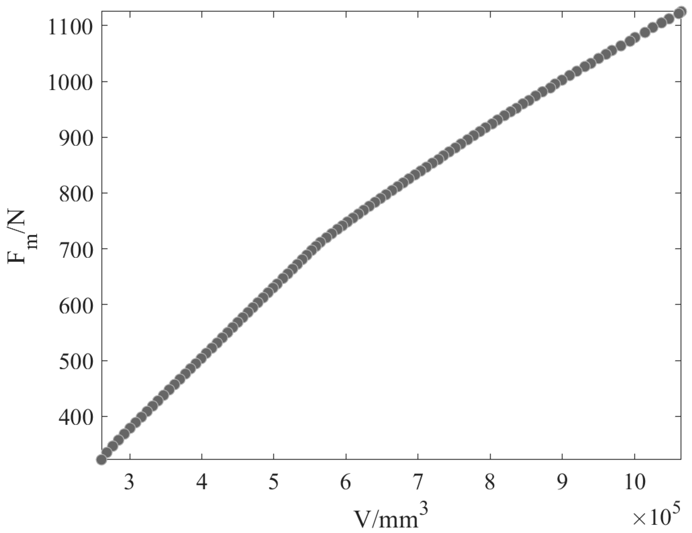
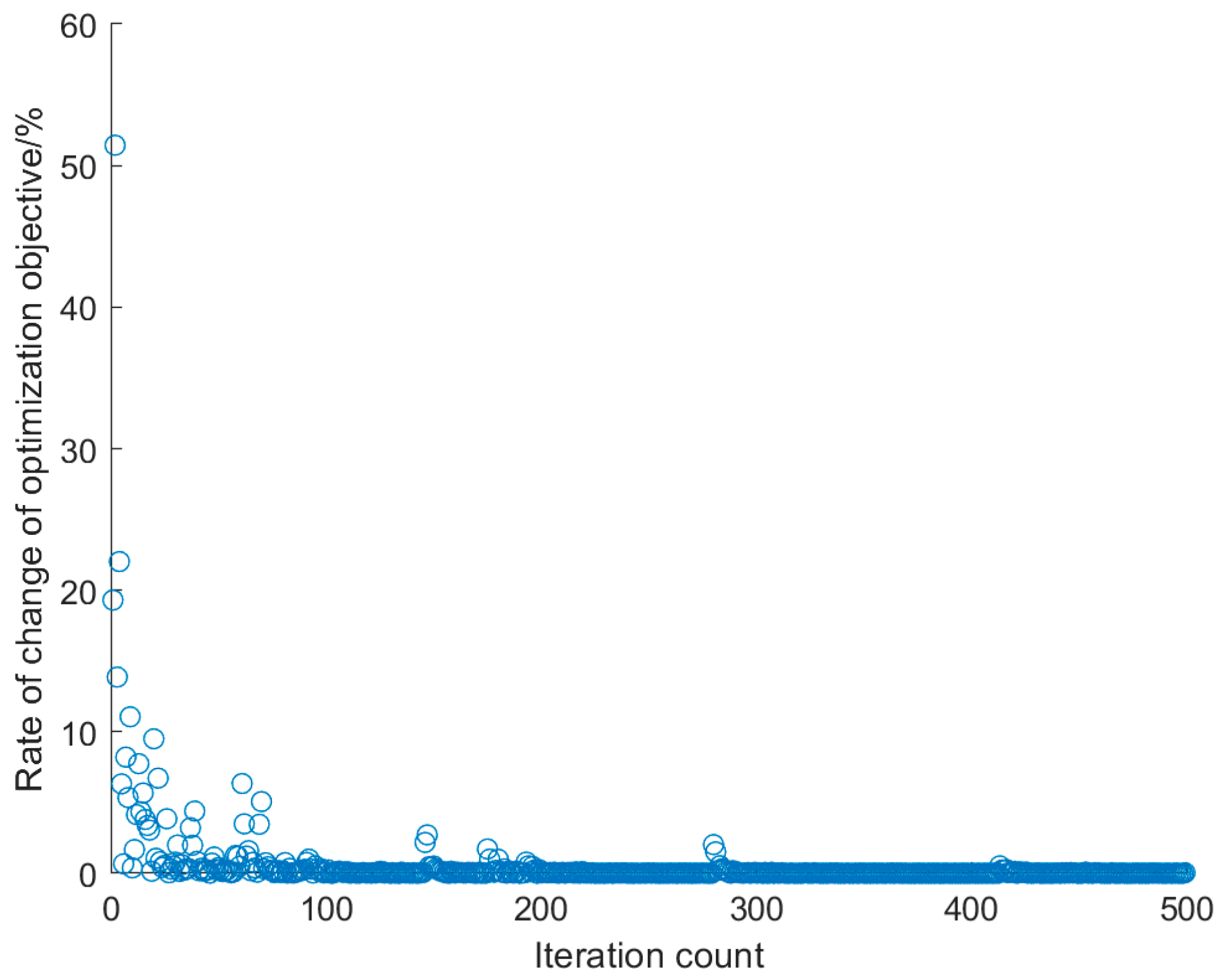
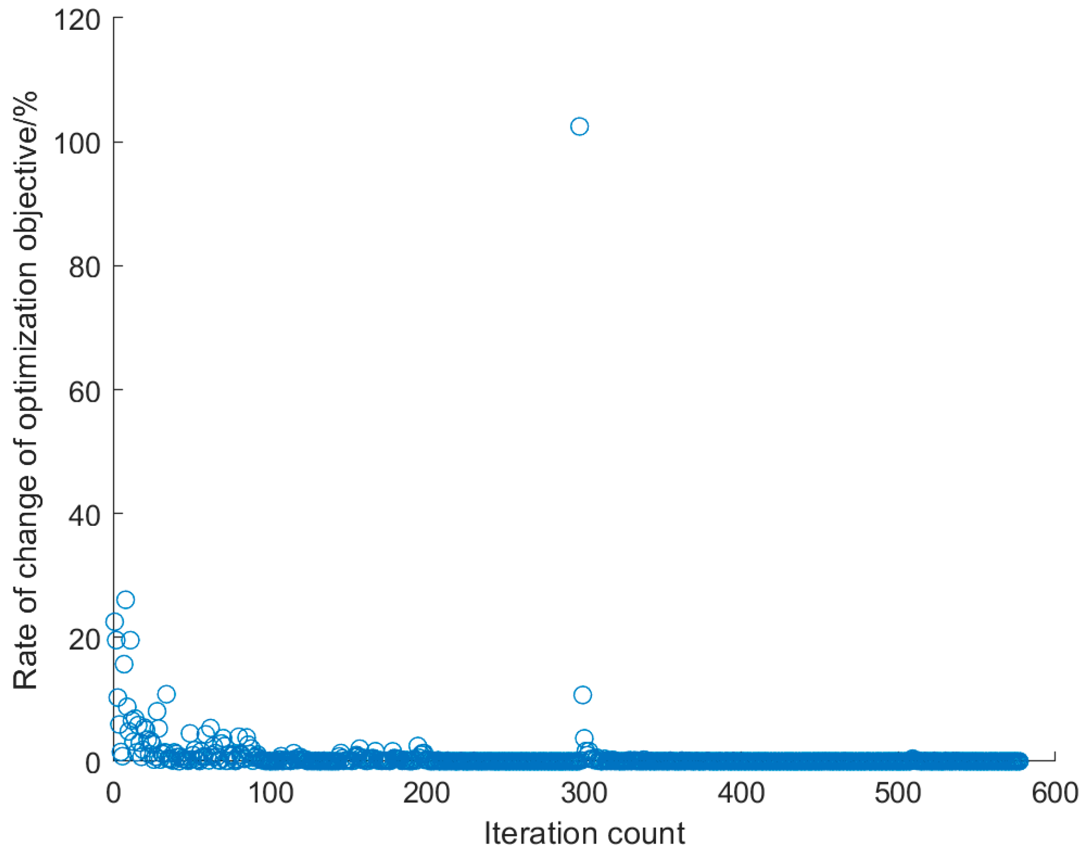
Based on the above-proposed constraints, optimization objective functions and optimization parameters, the Pareto-optimal solution set generated by MOEA/D with a population size of 100 after 500 iterations is as illustrated in Figure 4. The Pareto-optimal solution set in Figure 4 is relatively uniformly distributed. The convergence behavior of the algorithm is represented by the rate of change in the average value of the optimization objectives at each iteration, as shown in Figure 5.

4. Optimization of RAMB Using MOEA/D-Pref

The proposed MOEA/D-Pref is inspired by MOEA/D and constructed upon its foundational framework. Since only information from neighboring subproblems is utilized during the optimization of each individual subproblem, MOEA/D features relatively low computational complexity [28]. MOEA/D explores the Pareto-optimal front using predefined weight vectors. Changing the distribution of the weight vectors will also change the distribution of the Pareto-optimal solution set, which can be used to achieve a distribution that meets certain preferences.
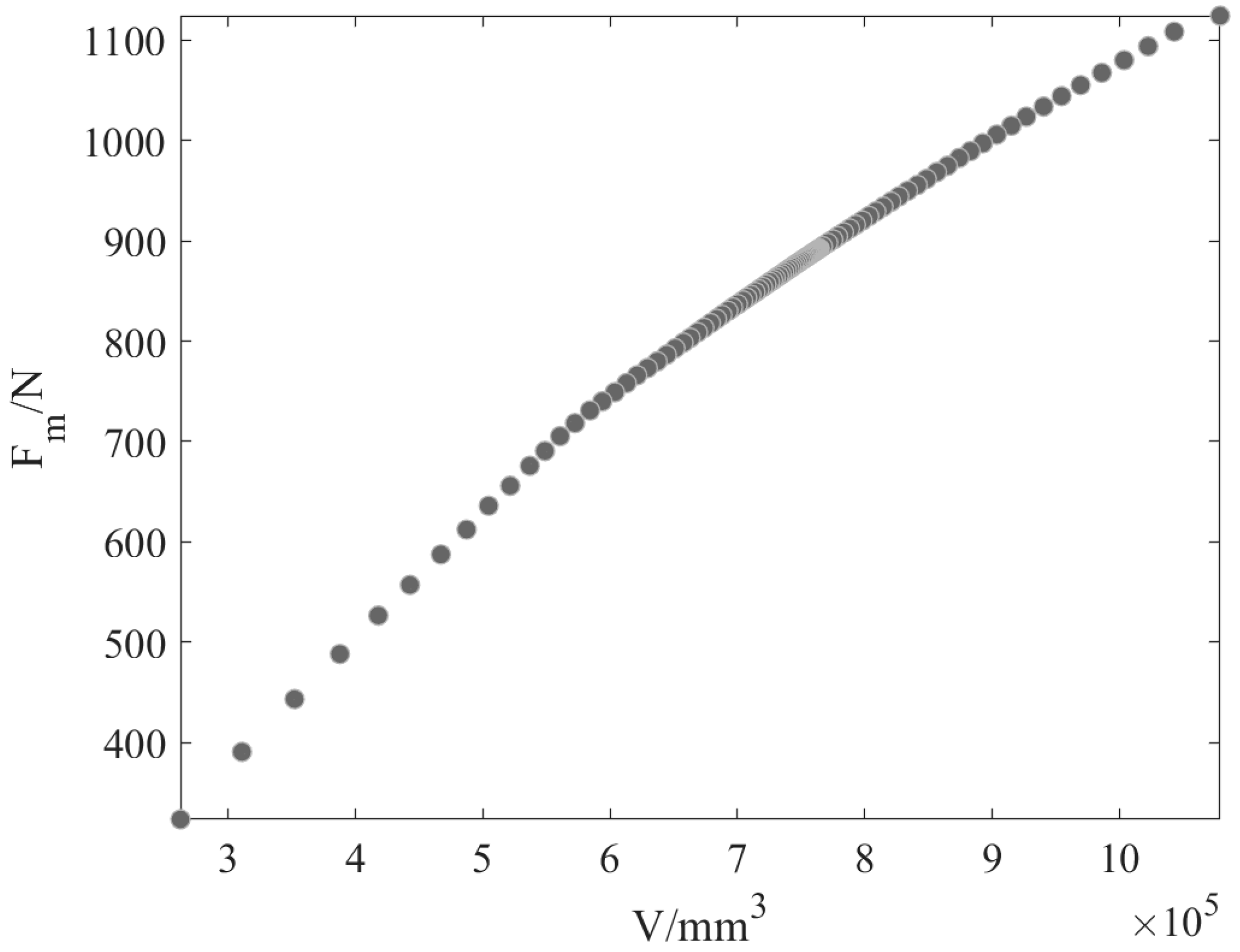
In Figure 4, the load capacity of the RAMB exhibits a positive correlation with its volume. When determining the target load capacity value F0, potential impacts on the RAMB have already been considered. Consequently, Pareto-optimal solutions with load capacities that are significantly higher or lower than F0 are typically disregarded by decision-makers. When selecting the most suitable Pareto-optimal solution from the set as the final optimal design, decision-makers generally prefer solutions where the load capacity is close to the target value F0. This paper proposes MOEA/D-Pref. The resulting Pareto-optimal solution set generated by this algorithm exhibits a non-uniform distribution: solutions are densely clustered near the target load capacity F0 and become progressively sparser with increasing distances from F0. Such a distributed Pareto-optimal solution set is more convenient in enabling decision-makers to make decisions.
The calculation of the load capacity targets must account for (1) the static load borne by the bearing in a given degree of freedom, (2) dynamic loads caused by rotor mass imbalance during rotation and (3) potential overload conditions. The calculation formula is expressed as
F 0 = k a k m G sh
where Gsh is the weight of the rotating shaft, ka is the core laminated coefficient, and km is a static load coefficient that takes into account dynamic loads and potential impacts based on the application requirements.
Under the conditions of ka = 0.98, km = 4.5 and Gsh = 204 N, F0 is calculated as 899 N. In fact, F0 is an estimated value calculated according to design experience; for simplicity, F0 is further estimated as 900 N.
The MOEA/D-Pref algorithm employs uniformly distributed weight vectors during its initial iterations. After completing a specified number Q of iterations, the algorithm begins recording the solution index i that exhibits the closest load capacity to the target value F0 in each subsequent iteration. When this index i remains unchanged for n consecutive iterations, MOEA/D-Pref switches to using non-uniformly distributed weight vectors to conduct the remainder of the optimization process. When the order of the optimal solution set remains unchanged for n consecutive iterations, the iterations end.
The distribution of the optimal solution set obtained by MOEA/D is determined by the weight vectors. By adjusting the weight vectors, the Pareto-optimal solution set transitions from a uniform distribution to a clustered distribution around the position of the i-th weight vector. This non-uniform redistribution of weight vectors can be achieved through exponential function mapping, with the operational formula expressed as
W k j = W i j × S ^ ( ( W k j W i j ) ) j = 2 , 1 k i W k j = W k j j = 1 , 1 k i W k j = W i j × S ^ ( ( W k j W i j ) ) j = 1 , i + 1 k N W k j = W k j j = 2 , i + 1 k N W k j * = W k j j = 1 2 W k j 1 k N
where W* represents the non-uniform weight vectors, W represents the uniformly distributed weight vectors, N is the population size and S is a scaling factor.
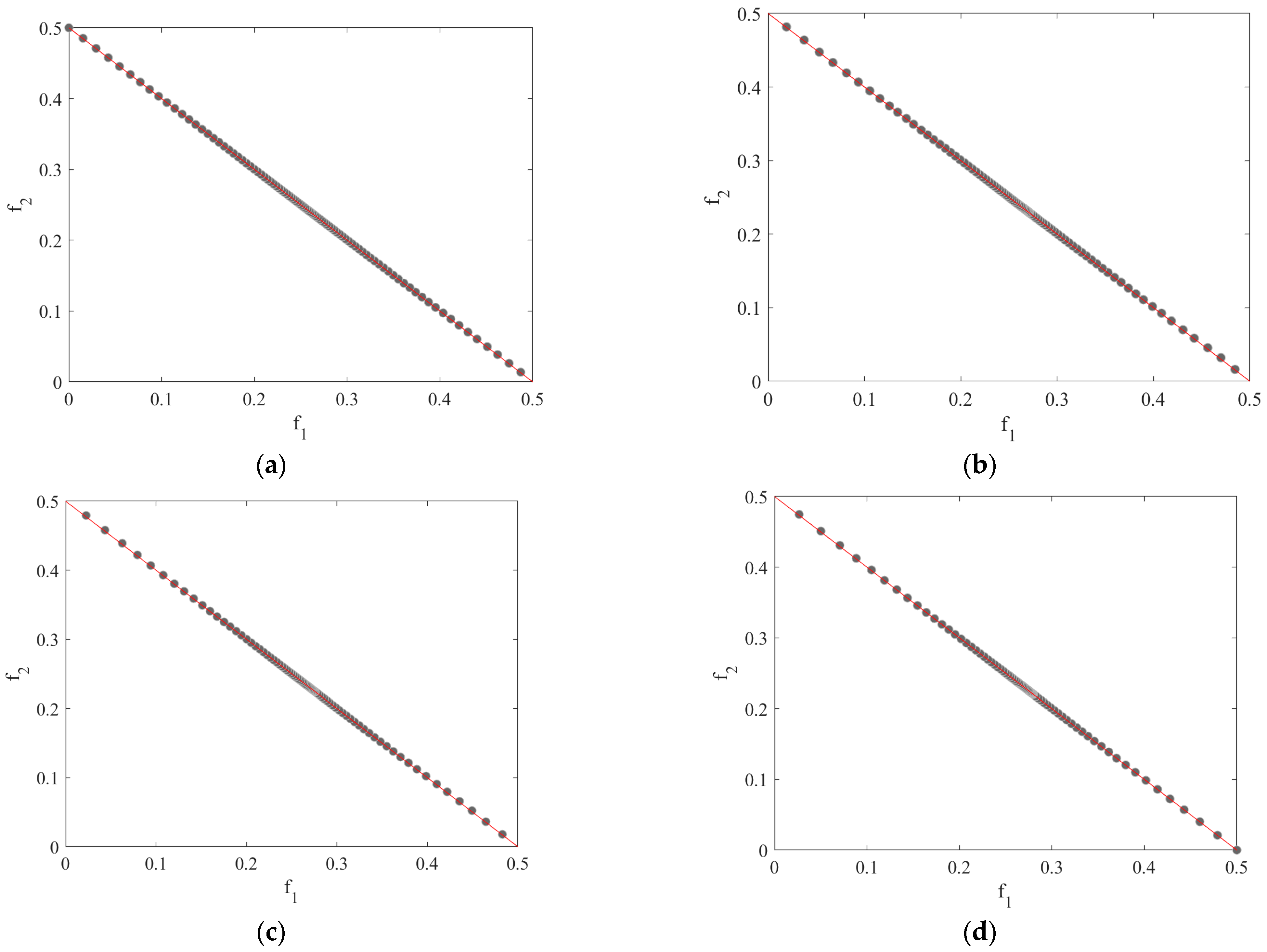
When the scaling factor S ≥ 1, the clustering effect becomes increasingly pronounced with higher S values. To validate the rationality of Equation (20), tests were conducted under the conditions of N = 100 and i = 50, verifying the cases for S = 2, S = 3, S = 4 and S = 5. The distribution of the weight vectors is illustrated in Figure 6.
As illustrated in Figure 6, the clustering effect exhibits a positive correlation with increasing S values. To quantitatively validate this observation, the spacing of these non-uniformly distributed weight vectors is calculated, as listed in Table 1. The formula for the spacing can be expressed as
s p a c i n g = 1 N i = 1 N ( d ¯ d i ) 2
where N is the number of weight vectors, di is the Euclidean distance between weight vector i and its nearest weight vector and d ¯ is the average of these Euclidean distances.
The larger the value of the spacing, the more uneven the distribution of the weight vectors. From the data in Table 1, it can be seen that the value of S has a strong positive correlation with the unevenness of the weight vector distribution. The distribution of the weight vectors represents the distribution of Pareto-optimal solutions. The clustering effect becomes increasingly pronounced with higher values of S, while concurrently causing the progressive blurring of the Pareto front’s topological features. For convenience in determining the value of S, the distribution of the optimal solution set for the test function DTLZ1 (Deb–Thiele–Laumanns–Zitzler 1) is shown in Figure 7 for the cases of S = 2, 3, 4, 5.
The optimal distribution can be achieved by changing the size of S. According to Figure 7, when S = 2, S = 3, S = 4 and S = 5, the optimal solution distribution of DTLZ1 is concentrated in the middle position. The value of S is determined by the decision-maker’s preference, and the distribution when S = 3 satisfies the decision-maker’s preference. In subsequent optimizations, the value of S is 3.
Based on the rotor weight and possible external impacts, the target value of the load capacity is set at 900 N. The Pareto-optimal solution set obtained using MOEA/D-Pref for the optimization of RAMBs is shown in Figure 8. In the case of Q = 100, n = 5, N = 100 and S = 3, at the 298th iteration, the algorithm determines i to be 34. The Pareto-optimal solution set after 573 iterations is densely distributed near the target value and sparsely distributed away from the target value, while ensuring a complete Pareto front. The convergence behavior of the algorithm is represented by the rate of change in the average value of the optimization objective at each iteration, as shown in Figure 8. The rate of change in Figure 9 exhibits drastic changes at the initial iterations and near the 298th iteration.
The optimal design of the 12-pole RAMB is selected from the set of optimal solutions calculated for 12-pole RAMBs using MOEA/D-Pref. The load capacity target value is determined with consideration of potential external impacts. An optimal solution is considered to meet the design requirements when its load capacity exceeds this target value. Under these conditions, the optimization strategy prioritizes volume minimization as the primary selection criterion. It should be noted that the load capacity calculation formula derived from the magnetic circuit method, which neglects non-linear factors, provides an estimated value. Since this method disregards the magnetic reluctance of both stator and rotor core materials, the calculated load capacity may be overestimated compared to actual performance situations. To ensure reliable compliance with the target requirement, the selected optimal solution must maintain a bearing capacity that exceeds the target value by a safe margin based on design experience.
The optimal solution that exceeds the target load capacity value and is close to the target load capacity value is considered a selectable solution.
The numbers of selectable solutions calculated by MOEA/D and MOEA/D-Pref under different margins are listed in Table 2. In the multi-objective optimization of the 12-pole RAMB, the number of iterations using MOEA/D without preference is 298, and the number of iterations using MOEA/D-Pref is 573. Although MOEA/D-Pref requires more iterations than MOEA/D for the multi-objective optimization of RAMBs, MOEA/D-Pref has a significant advantage in terms of the number of selectable solutions that it generates. If the population size in MOEA/D is increased to generate the same number of selectable solutions as in MOEA/D-Pref, the computational load will also increase. The computational load is characterized by the code execution time on the same machine. To enable MOEA/D and MOEA/D-Pref to generate the same number of selectable solutions, the percentage ratio of the computational load of MOEA/D-Pref to that of MOEA/D based on 40 independent runs is calculated, as listed in Table 3. The data in Table 3 show that the period of 126 s required for MOEA/D-Pref to generate five selectable solutions is 38% of that required by MOEA/D when the feasible solution domain is between 900 N and 910 N. As the selectable solution range increases, this ratio rises; however, within a reasonable selectable solution range, this ratio remains less than 1, indicating that the computational load required by MOEA/D-Pref is less than that required by MOEA/D.

5. Optimal Design of 12-Pole RAMB

Based on the above selection method, an optimal solution is selected, and the parameters for the optimized RAMB are shown in Table 4.
According to Table 4, a model was constructed in finite element simulation software. Figure 10 presents the magnetic flux line distribution and magnetic flux density distribution of the RAMB when the bias current excitation is applied. Mesh independence was verified by progressively refining the grid until the difference in magnetic flux density in the air gap between two consecutive refinements was less than 3%. According to Equation (2), the air gap magnetic flux density under each pole should be 0.45 T under bias current excitation. Table 5 presents the magnetic flux density at five air gap locations under the magnetic poles, calculated using the finite element method. These locations are marked in Figure 10b. The simulation results demonstrate that the magnetic circuit coupling between individual pole units is relatively low.
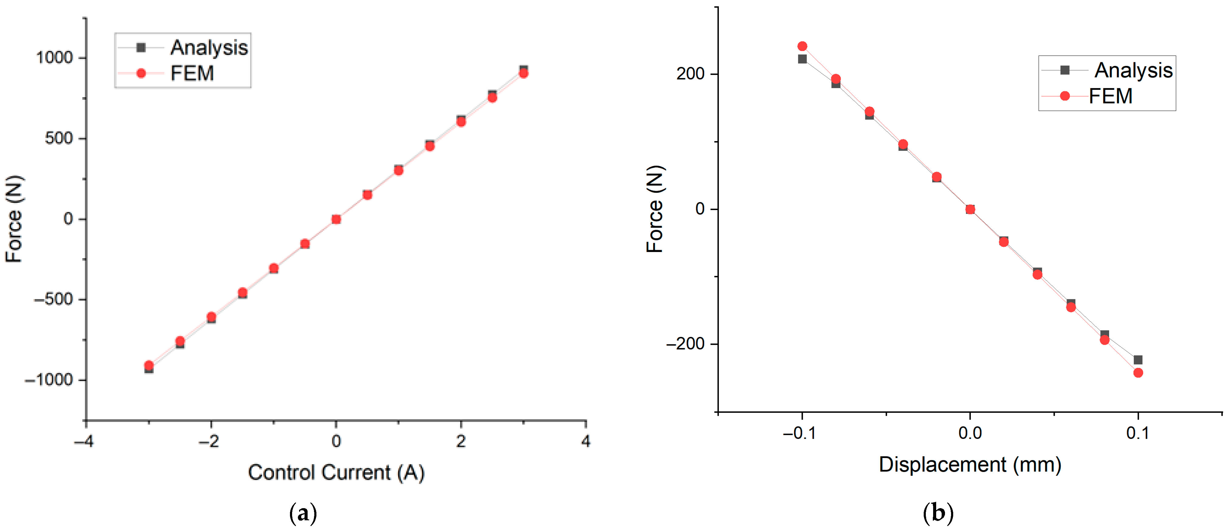
The volume of the optimized RAMB is calculated to be 817,620 mm3 using Equation (12) and 823,200 mm3 using the finite element method, with a difference of 0.67%. The relatively low volume error may be due to the estimation of the magnetic pole area, and it verifies the reliability of the volume formula. Based on Table 4, the load capacity of the optimized RAMB is calculated to be 927 N using the magnetic circuit method and 906.3 N using the finite element method, with a difference of 2.3%. The load capacity calculated using the finite element method exceeds the target value, and the optimized design meets the load capacity requirements. The force generated per unit control current while maintaining a constant air gap length is the current stiffness coefficient. Based on the established mathematical model, the ratio of the load capacity to the maximum control current in the coils is approximately equal to the current stiffness coefficient. When the rotor is not offset, the current stiffness coefficient of the optimized RAMB is calculated to be 309 N/A using the magnetic circuit method and 302 N/A using the finite element method, with a difference of 2.3%, as shown in Figure 11a. The force variation per unit rotor displacement under a constant control current is the displacement stiffness coefficient. When the control current is equal to 0, the displacement stiffness coefficient of the optimized RAMB is calculated to be −2317 N/mm using the magnetic circuit method and −2412 N/mm using the finite element method, with a difference of 3.9%. These results are shown in Figure 11b. These differences, being less than 4%, are relatively low and verify the reliability of the mathematical model established.

6. Conclusions

Based on the phenomenon in which decision-makers may be more interested in Pareto-optimal solutions with a load capacity near the target value, in order to enable decision-makers to select the most suitable optimal solution, this paper proposes MOEA/D-Pref for the optimization of RAMBs. The proposed algorithm generates a non-uniformly distributed Pareto-optimal solution set, with a higher solution density in the region of interest; it features a simple and efficient program structure, characterized by straightforward implementation.
The proposed algorithm was applied to optimize a 12-pole RAMB, and the obtained Pareto front also verifies the effectiveness of the algorithm. The difference between the current stiffness coefficients of the optimized RAMB, calculated by the proposed algorithm and by the finite element method, is 2.3%. The difference between the displacement stiffness coefficients of the optimized RAMB, calculated by the proposed algorithm and by the finite element method, is 3.9%. These differences, being less than 4%, are relatively low, verifying the reliability of the mathematical model established.
The optimization steps for RAMBs described in this paper can provide a reference for the optimal design of magnetic bearings. The mechanism for introducing preference information in MOEA/D-Pref can provide a reference for preference-based multi-objective optimization algorithms.
In future research, the finite element method can be used to take into account non-linear factors in magnetic bearings [29], which would help to improve the accuracy. Applying the finite element method to multi-objective optimization design will become the focus of further research. Moreover, multi-objective optimization has shown effectiveness in other industrial domains, such as EV smart charging systems [30], achieving balanced performance across competing objectives. The application of multi-objective optimization integrated with preference mechanisms in other fields is another direction for future research.

Author Contributions

Conceptualization, X.L.; methodology, X.L. and X.W.; software, X.L. and H.S.; validation, X.L. and H.S.; formal analysis, X.L. and X.W.; data curation X.L.; writing—original draft preparation, X.L.; writing—review and editing, X.W. and X.L.; supervision, X.W. All authors have read and agreed to the published version of the manuscript.

Funding

This research received no external funding.

Institutional Review Board Statement

Not applicable.

Informed Consent Statement

Not applicable.

Data Availability Statement

The original contributions presented in the study are included in the article, further inquiries can be directed to the corresponding author.

Conflicts of Interest

The authors declare no conflicts of interest.

References

  1. Le, Y.; Wang, D.; Zheng, S.Q. Design and optimization of a radial magnetic bearing considering unbalanced magnetic pull effects for magnetically suspended compressor. IEEE Trans. Mechatron. 2022, 27, 5760–5770. [Google Scholar] [CrossRef]
  2. Zheng, S.; Wang, C. Rotor balancing for magnetically levitated TMPs integrated with vibration self-sensing of magnetic bearings. IEEE Trans. Mechatron. 2021, 26, 3031–3039. [Google Scholar] [CrossRef]
  3. Han, X.; Liu, G.; Le, Y.; Dong, B.T.; Zheng, S.Q. Unbalanced magnetic pull disturbance compensation of magnetic bearing systems in MSCCs. IEEE Trans. Ind. Electron. 2023, 70, 4088–4097. [Google Scholar] [CrossRef]
  4. Jastrzebski, R.P.; Liukkonen, O. Analysis of a segmented axial active magnetic bearing for multi-MW compressor applications. IEEE Trans. Mechatron. 2023, 28, 2799–2809. [Google Scholar] [CrossRef]
  5. Zhang, R.; Song, X.Y.; Cui, Z.Z.; Hao, W.; Xu, C.; Song, L.W. Distributed modeling of isolated active magnetic bearings considering magnetic leakage and material nonlinearity. Energies 2023, 16, 8023. [Google Scholar] [CrossRef]
  6. Moser, R.; Sandtner, J.; Bleuler, H. Optimization of repulsive passive magnetic bearings. IEEE Trans. Magn. 2006, 42, 2038–2042. [Google Scholar] [CrossRef]
  7. Cheng, S.B.; Olles, M.W.; Burger, A.F.; Day, S.W. Optimization of a hybrid magnetic bearing for a magnetically levitated blood pump via 3-D FEA. Mechatronics 2011, 21, 1163–1169. [Google Scholar] [CrossRef]
  8. Sun, Y.K.; Yin, S.J.; Yuan, Y.; Huang, Y.H. Multi-objective optimization design of magnetic bearing based on genetic particle swarm optimization. Prog. Electromagn. Res. M 2019, 81, 181–192. [Google Scholar] [CrossRef]
  9. Zhang, H.; Zhu, H.Q.; Wu, M.Y. Multi-Objective Parameter Optimization-Based Design of Six-Pole Radial Hybrid Magnetic Bearing. IEEE J. Emerg. Sel. Top. Power Electron. 2022, 10, 4526–4535. [Google Scholar] [CrossRef]
  10. Wang, Y.B.; Cao, J.W.; Chen, B.; Chen, X.; Liu, J.X.; Li, L.Y. Multi-objective Parameter Optimization Design of Radial Magnetic Levitation Bearing. In Proceedings of the 2024 27th International Conference on Electrical Machines and Systems (ICEMS), Fukuoka, Japan, 26–29 November 2024. [Google Scholar]
  11. Jin, Z.J.; Sun, X.D.; Chen, L.; Yang, Z.B. Robust Multi-Objective Optimization of a 3-Pole Active Magnetic Bearing Based on Combined Curves with Climbing Algorithm. IEEE Trans. Ind. Electron. 2022, 69, 5491–5501. [Google Scholar] [CrossRef]
  12. Zhong, W.; Palazzolo, A.; Kang, X. Multi-Objective optimization design of nonlinear magnetic bearing rotor dynamic system. J. Vib. Acoust. Trans. ASME 2017, 139, 011011. [Google Scholar] [CrossRef]
  13. Rao, J.S.; Tiwari, R. A pareto optimal design analysis of magnetic thrust bearings using multi-objective genetic algorithms. Int. J. Comput. Methods Eng. Sci. Mech. 2015, 16, 71–85. [Google Scholar] [CrossRef]
  14. Yadav, V.K.; Kumar, P.; Bhushan, G. A novel approach for design optimisation of radial active magnetic bearing. Aust. J. Mech. Eng. 2023, 21, 1461–1473. [Google Scholar] [CrossRef]
  15. Deb, K.; Pratap, A.; Agarwal, S.; Meyarivan, T. A fast and elitist multiobjective genetic algorithm: NSGA-II. IEEE Trans. Evol. Comput. 2002, 6, 182–197. [Google Scholar] [CrossRef]
  16. Zhang, Q.F.; Li, H. MOEA/D: A multiobjective evolutionary algorithm based on decomposition. IEEE Trans. Evol. Comput. 2007, 11, 712–731. [Google Scholar] [CrossRef]
  17. Zhang, X.Y.; Tian, Y.; Jin, Y.C. A knee point driven evolutionary algorithm for many-objective optimization. IEEE Trans. Evol. Comput. 2014, 19, 761–776. [Google Scholar] [CrossRef]
  18. Bozorgi, S.M.; Yazdni, S. IWOA: An improved whale optimization algorithm for optimization problems. J. Comput. Des. Eng. 2019, 6, 243–259. [Google Scholar] [CrossRef]
  19. Deb, K.; Jain, H. An evolutionary many-objective optimization algorithm using reference-point-based nondominated sorting approach, part I: Solving problems with box constraints. IEEE Trans. Evol. Comput. 2013, 18, 577–601. [Google Scholar] [CrossRef]
  20. Molina, J.; Santana, L.V.; Hernández-Díaz, A.G.; Coello, C.A.; Caballero, R. g-dominance: Reference point based dominance for multiobjective metaheuristics. Eur. J. Oper. Res. 2009, 197, 685–692. [Google Scholar] [CrossRef]
  21. Said, L.B.; Bechikh, S.; Ghedira, K. The r-Dominance: A New Dominance Relation for Interactive Evolutionary Multicriteria Decision Making. IEEE Trans. Evol. Comput. 2010, 14, 801–818. [Google Scholar] [CrossRef]
  22. Zheng, J.H.; Xie, Z.H. A Study on How to Use Angle Information to Include Decision Maker’s Preferences. Acta Electron. Sin. 2014, 42, 2239–2246. [Google Scholar]
  23. Mohammadi, A.; Omidvar, M.N.; Li, X.D. Reference point based multi-objective optimization through decomposition. In Proceedings of the 2012 IEEE Congress on Evolutionary Computation, Brisbane, QLD, Australia, 10–15 June 2012. [Google Scholar]
  24. Li, Y.; Sheng, C.; Zhang, B.; Zhao, Q.; Du, G.F. Optimization Design of Electromagnetic Bearing for Long-life Centrifugal Pump. In Proceedings of the 3rd International Conference on Mechatronics Technology and Aerospace Engineering (ICMTAE), Nanchang, China, 15–17 September 2023. [Google Scholar]
  25. Fang, J.; Wang, C.; Wen, T. Design and optimization of a radial hybrid magnetic bearing with separate poles for magnetically suspended inertially stabilized platform. IEEE Trans. Mechatron. 2014, 50, 8101011. [Google Scholar]
  26. Chang, Y.T.; Luo, W.J.; Lin, X.; She, Z.N.; Shi, Y.H. Multiparty multiobjective optimization by MOEA/D. In Proceedings of the 2022 IEEE Congress on Evolutionary Computation (CEC), Padua, Italy, 18–23 July 2022. [Google Scholar]
  27. Gulec, M.; Yolacan, E.; Aydin, M. Design and control of an 8-slot radial flux magnetic bearing. In Proceedings of the 2014 Power Electronics, Electrical Drives, Automation and Motion (SPEEDAM), Ischia, Italy, 18–20 June 2014. [Google Scholar]
  28. Zhu, X.Q.; Gao, Z.H.; Du, Y.M.; Cheng, S.X.; Fang, X. A decomposition-based multi-objective optimization approach considering multiple preferences with robust performance. Appl. Soft Comput. 2018, 73, 263–282. [Google Scholar] [CrossRef]
  29. Stumberger, G.; Dolinar, D.; Palmer, U. Optimization of radial active magnetic bearings using the finite element technique and the differential evolution algorithm. IEEE Trans. Magn. 2020, 36, 1009–1013. [Google Scholar]
  30. Borozan, S.; Giannelos, S.; Aunedi, M.; Strbac, G. Option Value of EV Smart Charging Concepts in Transmission Expansion Planning under Uncertainty. In Proceedings of the 21st Mediterranean Electrotechnical Conference (MELECON), Palermo, Italy, 14–16 June 2022. [Google Scholar]
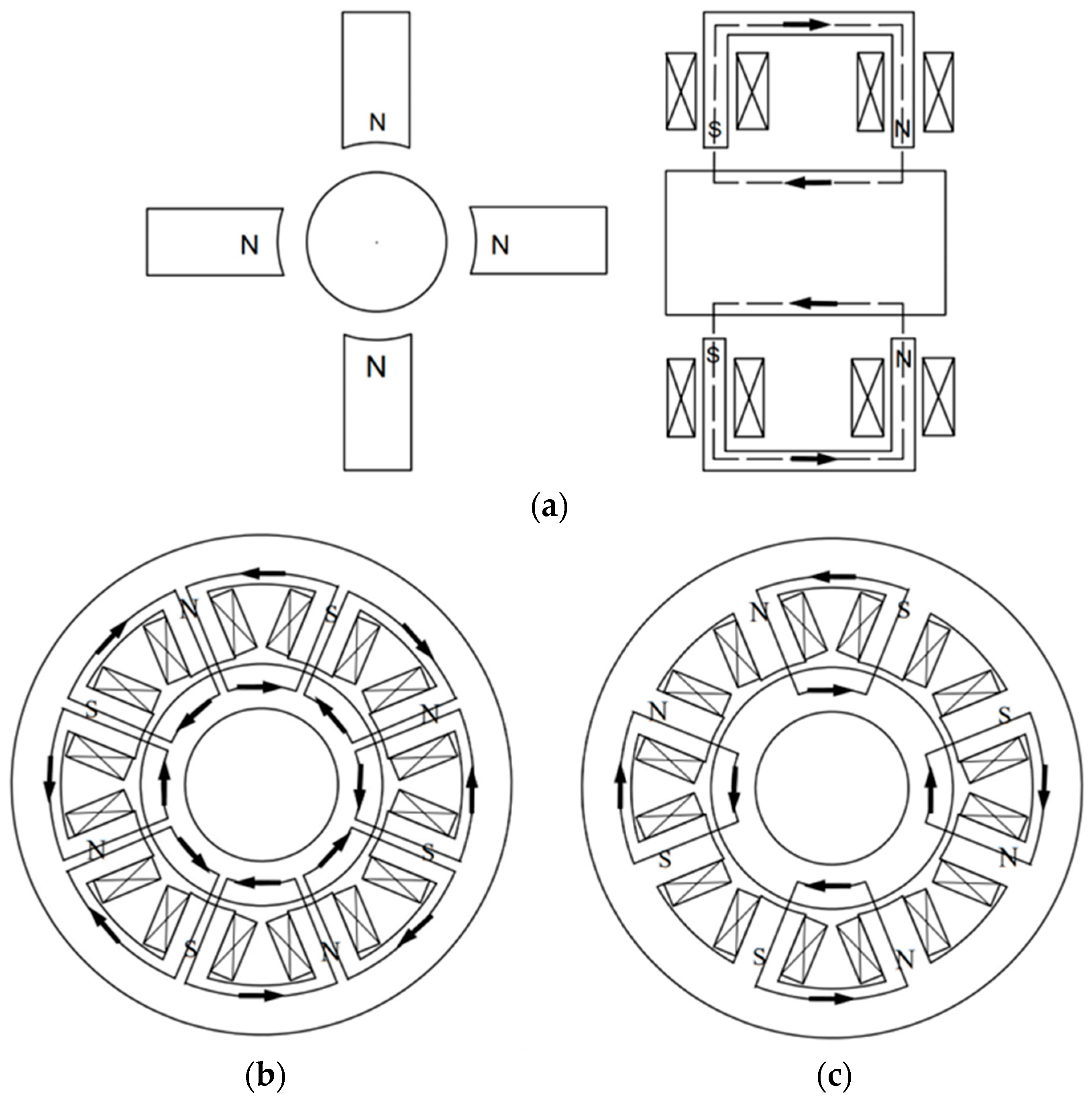
Figure 1. (a) A homopolar RAMB; (b) a coupled heteropolar RAMB; (c) a decoupled heteropolar RAMB.
Energies 18 04299 g001
Figure 2. The structure and magnetic circuit of a 12-pole heteropolar decoupled RAMB.
Energies 18 04299 g002
Figure 3. The structure of the RAMB.
Energies 18 04299 g003
Figure 4. Pareto front of MOEA/D.
Energies 18 04299 g004
Figure 5. The rate of change in the average value of the optimization objective of MOEA/D.
Energies 18 04299 g005
Figure 6. The distribution of the weight vectors: (a) S = 2; (b) S = 3; (c) S = 4; (d) S = 5.
Energies 18 04299 g006
Figure 7. The distribution of the optimal solution set for DTLZ1: (a) S = 2; (b) S = 3; (c) S = 4; (d) S = 5.
Energies 18 04299 g007
Figure 8. Pareto front of MOEA/D-Pref.
Energies 18 04299 g008
Figure 9. The rate of change in the average value of the optimization objective of MOEA/D-Pref.
Energies 18 04299 g009
Figure 10. (a) Magnetic flux line diagrams; (b) magnetic flux density diagrams.
Energies 18 04299 g010
Figure 11. (a) Current stiffness coefficient; (b) displacement stiffness coefficient.
Energies 18 04299 g011
Table 1. Spacing of non-uniformly distributed weight vectors.
SSpacing
20.0090
30.0113
40.0130
50.0145
60.0156
70.0167
80.0177
Table 2. The number of selectable solutions.
Load Capacity RangeNumber of Selectable Solutions by MOEA/DNumber of Selectable Solutions by MOEA/D-Pref
900 N–910 N15
900 N–920 N29
900 N–930 N412
900 N–940 N514
900 N–950 N616
Table 3. Comparison of computational load between MOEA/D and MOEA/D-Pref.
Load Capacity RangePercentage Ratio of Computational Load of MOEA/D-Pref to that of MOEA/D
900 N–910 N38%
900 N–920 N42%
900 N–930 N64%
900 N–940 N69%
900 N–950 N72%
Table 4. The fundamental parameters for the optimized RAMB.
ParameterValue
Rotor inner diameter/mm65.2
Rotor outer diameter/mm91.2
Stator inner diameter/mm92
Stator outer diameter/mm160.2
Axial length/mm60
Main pole width/mm26
Angle between centerlines of main and secondary poles/deg33
Bias current/A3
Maximum control current/mm3
Maximum current density/A/mm23.5
Number of turns of coil on main pole53
Number of turns of coil on secondary pole43
Load capacity/N927
Volume/mm3817620 mm3
Current stiffness coefficient/N/A309 N/A
Displacement stiffness coefficient/N/mm−2317 N/mm
Table 5. Magnetic flux densities at five air gap locations under the magnetic poles.
12345
B (T)0.45430.44610.44650.45320.4481
Disclaimer/Publisher’s Note: The statements, opinions and data contained in all publications are solely those of the individual author(s) and contributor(s) and not of MDPI and/or the editor(s). MDPI and/or the editor(s) disclaim responsibility for any injury to people or property resulting from any ideas, methods, instructions or products referred to in the content.