Article

Acoustic-Based Condition Recognition for Pumped Storage Units Using a Hierarchical Cascaded CNN and MHA-LSTM Model

1
Fujian Xianyou Pumped Storage Power Co., Ltd., Putian 351267, China
2
State Key Laboratory of Regional and Urban Ecology, Xiamen Key Lab of Urban Metabolism, Research Center of Urban Carbon Neutrality, Institute of Urban Environment, Chinese Academy of Sciences, Xiamen 361021, China
3
Unisound AI Technology Co., Ltd., Xiamen 361022, China
*
Authors to whom correspondence should be addressed.
Energies 2025, 18(16), 4269; https://doi.org/10.3390/en18164269
Submission received: 14 July 2025 / Revised: 7 August 2025 / Accepted: 8 August 2025 / Published: 11 August 2025

Abstract

As an important regulating resource in power systems, pumped storage units frequently switch operating conditions due to peak shaving and frequency regulation, making the condition transitions complex. Traditional methods struggle to achieve high-precision classification. This paper proposes a hierarchical cascade deep learning model based on noise signals, which integrates a convolutional neural network (CNN) with a multi-head attention long short-term memory network (MHA-LSTM) to address the differentiated recognition of steady-state and transitional conditions. The CNN efficiently extracts multi-scale spatial features from sound spectrograms, enabling fast classification under steady-state conditions. The MHA-LSTM combines attention mechanisms with time-series modeling. This enhances its ability to capture long-range dependencies in the signals. And it significantly improves classification accuracy in ambiguous boundaries and transitional scenarios. Testing on 3413 noise samples shows that the proposed method achieves an overall accuracy of 92.22%, with steady-state condition recognition exceeding 98%, and recall and F1 score above 90% for major categories. Compared with other approaches, this model provides a high-precision classification tool for unit health monitoring, supporting the intelligent operation and maintenance of power plants.

1. Introduction

Energy is the driving force behind human production and daily life, and a foundation for global development [1]. As the challenges of climate change become more severe, energy transition has become a global consensus. Many countries are accelerating the development of clean energy and shifting from traditional energy systems to those dominated by renewables. As one of the world’s largest energy markets, China has not only set strategic goals for “carbon peaking” and “carbon neutrality” [2] but also outlined its 14th Five-Year Plan [3], which states that the combined installed capacity of wind and solar power will exceed 1.2 billion kilowatts by 2030. Achieving this goal marks a major step forward in China’s energy transition and places higher demands on the flexibility and stability of the power system. However, the intermittent and fluctuating nature of renewable energy can pose serious risks to grid stability. Therefore, enhancing the grid’s regulation and energy storage capabilities has become a critical challenge.
As a key component of the power system and an efficient solution for large-scale energy storage [4], pumped storage power stations play an important role in peak shaving, frequency regulation, and maintaining grid stability. By the end of 2024, the total installed capacity of pumped storage power stations in China had reached 58.69 GW, ranking first in the world and accounting for approximately 30% of the global total. According to the 14th Five-Year Plan, the cumulative installed capacity is expected to reach around 120 GW by 2030. However, the rapid expansion in scale is accompanied by increasing challenges in operational management. These stations experience frequent starts and stops, and their operating conditions are highly complex, influenced by hydraulic, mechanical, and electrical factors [5]. Under such heavy-duty operation, performance degradation is likely to occur. Minor degradation can affect plant lifespan and grid stability, while severe degradation may lead to major economic losses and serious safety incidents [6], This poses significant challenges for the monitoring and maintenance of equipment. To ensure the safe and stable operation of pumped storage units, it is essential to build an efficient condition monitoring system and accurately identify the working states of key components. Currently, the construction and operation of pumped storage stations are gradually shifting toward automation and intelligent management [7]. Traditional maintenance methods, which rely on periodic inspections, can no longer meet the high reliability and efficiency demands of modern power plants. In contrast, predictive maintenance based on real-time monitoring is becoming the mainstream approach. By continuously monitoring the operating status of hydroelectric units and applying intelligent analysis, more efficient equipment management can be achieved. However, most existing studies focus on the coarse classification of operating conditions, such as load variation, shutdown, or speed change [8], These broad categories fail to capture the detailed behavior of units under complex conditions, limiting the accuracy and sensitivity of diagnostics.
Traditional condition identification methods for pumped storage units include rule-based expert systems [9], spectrum analysis [10], and fuzzy recognition techniques [11]. However, as operating conditions become more complex, these traditional approaches face limitations in terms of real-time performance, accuracy, and generalization ability [12,13]. In recent years, the rapid development of deep learning has offered new solutions for intelligent condition monitoring of power equipment. With strong feature extraction and modeling capabilities, deep learning has been increasingly applied in industrial systems for status recognition. By automatically learning key features from raw signals, these models significantly improve the accuracy of condition identification under complex scenarios. Currently, unit condition monitoring mainly relies on sensors to collect data such as vibration, current, voltage, and temperature [14], and it uses machine learning or deep learning algorithms to classify operating states. In comparison, acoustic signals offer a non-contact, highly responsive data source, providing unique advantages in reflecting equipment conditions [15]. Studies have shown that sound can detect anomalies earlier than vibration signals [16]. However, research on using acoustic signals for condition recognition in pumped storage units remains limited, and there is still significant room for further exploration.
Among deep learning methods, CNNs have been widely used in condition monitoring for hydropower units due to their strong feature learning capabilities. A key advantage of CNN is the use of weight sharing in convolutional layers, which helps prevent overfitting. This structure reduces model complexity and significantly lowers the number of trainable parameters. CNNs have shown strong performance in handling signal data such as sound spectrograms [17]. Kumar et al. [18] developed an improved CNN model based on acoustic signals and applied it to bearing fault detection. However, CNNs are limited to learning static features and do not capture long-term dependencies in sequential data. This makes them less effective for processing long time-series inputs. To address this, Hochreiter et al. [19] proposed the LSTM network, an improved version of recurrent neural networks (RNNs), which is well suited to modeling sequential data. LSTM can learn long-term dependencies as an inherent part of its structure. Dao et al. [20] developed a BO+CNN+LSTM model that combines the strengths of CNN and LSTM, achieving over 90% accuracy in turbine fault diagnosis. Zhou et al. [21] used a CNN-LSTM model based on vibration signals to build a health status prediction framework for pumped storage units and successfully forecasted degradation trends. As a result, hybrid models that integrate CNN and LSTM have been widely adopted for the condition monitoring of hydropower equipment. These models leverage the strengths of both architectures, improving prediction performance and accuracy in complex monitoring tasks.
Although LSTM uses a gating mechanism to regulate information flow, there is still room for improvement in its architecture. In standard LSTM models, equal attention is given to all time steps during the sequence, making it difficult to distinguish between critical and non-critical segments. In recent years, the transformer architecture has gained popularity for its ability to capture complex nonlinear relationships in sequential data using self-attention mechanisms [22]. An extension of self-attention can be embedded into LSTM units to filter out important temporal information. This enhances the model’s ability to focus on key time steps. In the field of mechanical condition monitoring, some studies have already explored hybrid models that combine MHA with LSTM. Zhang et al. [23] used an MHA-LSTM model to predict the remaining useful life of motor bearings. Zhang et al. [24] also designed an MHA-BiLSTM model to predict acoustic logging curves, showing strong performance in capturing both nonlinear relationships and sequence patterns. These models have not yet been applied to condition identification in pumped storage units. Therefore, this study integrates MHA into the LSTM structure. The combination takes advantage of both mechanisms. The LSTM captures long-term dependencies in sequential data, while MHA highlights the most relevant features across the sequence.
The fine-grained recognition of operating conditions in pumped storage units is a complex multi-class classification task. At present, cascade-based methods are widely used to simplify such problems due to their strong hierarchical structuring capabilities. By using a hierarchical cascade framework, deep features can be extracted to solve complex sub-classification tasks, while simpler tasks can be handled using shallow features. Yang et al. [25] proposed a hierarchical framework based on cascade forests, which effectively matched features of different depths to corresponding fault types, significantly improving both classification performance and computational efficiency. Zhang et al. [26] developed a hierarchical diagnostic approach that combines an improved deep forest with case-based reasoning (CBR), and they successfully applied it to railway turnout fault diagnosis. These approaches offer valuable insights for multi-condition recognition in pumped storage units.
Based on the above discussion, under the complex condition transitions of pumped storage units, how to effectively combine acoustic signals with deep learning models to improve condition recognition accuracy remains a key challenge. Most existing studies focus on coarse-grained classification of conditions such as load variation, shutdown, or speed changes, and lack fine-grained recognition of the full operational process in pumped storage stations. Although machine learning has been applied to some extent in acoustic signal processing, the systematic condition classification of pumped storage units based on acoustic signals remains limited. This reveals a clear research gap that needs further exploration.
To address the gap mentioned above, this paper proposes an intelligent condition identification method for pumped storage units based on acoustic signals. The main contributions are as follows: (1) fully exploring the potential of acoustic signals in monitoring complex operating conditions, enabling effective recognition of multiple states in pumped storage units and (2) introducing a cascaded structure combining CNN and MHA-LSTM to build a deep learning model that integrates spatial and temporal features, thereby significantly improving the performance and robustness of condition identification.

2. Methods and Datasets

2.1. Method

2.1.1. Hierarchical Cascade

This study combines the strengths of CNN, LSTM, and MHA by proposing a two-stage cascaded hierarchical structure for the audio-based condition recognition of power plant equipment. The architecture fully leverages CNN’s advantage in extracting local time–frequency features and MHA-LSTM’s ability to model global dependencies in time series, thereby improving recognition accuracy and robustness under complex operating conditions.
The hierarchical strategy consists of two stages. First, the raw acoustic signals undergo preprocessing, including resampling, denoising, and short-time Fourier transform (STFT). The processed signals are then mapped to Mel spectrograms, which serve as input features for the CNN model. The CNN acts as a preliminary classifier in the first stage, primarily identifying whether the audio belongs to the “Shutdown Class II” category. “Shutdown Class II” refers to two shutdown conditions: generation shutdown and pumping shutdown. These conditions share strong pattern similarities and pose a high risk of confusion, thus requiring higher classification accuracy. If the CNN classifies an audio sample as “Shutdown Class II,” it is passed to the second-stage classifier, the MHA-LSTM module. This module first extracts 39-dimensional MFCC coefficients from the raw audio and concatenates them with 1-dimensional spectral flatness to form a 40-dimensional time-series feature. These features are then fed into the LSTM network to model temporal structures. An MHA mechanism is introduced to enhance the model’s focus on key time segments, enabling fine-grained classification between pumping shutdown and generation shutdown conditions. If the CNN classifies the sample as not belonging to “Shutdown Class II,” its result is directly taken as the final output. The detailed classification flow of this cascade structure is illustrated in Figure 1.
The algorithm was implemented using TensorFlow 2.1.0 in a Python 3.6.13 environment (Python Software Foundation, Wilmington, DE, USA). Audio processing and feature engineering were performed using the LibROSA library.

2.1.2. Convolutional Neural Network

CNN was first proposed by LeCun et al. and applied to handwritten digit recognition [27]. A convolutional neural network is a type of feedforward neural network inspired by the visual cortex cells in the brain. It achieves hierarchical automatic learning of spatial features through local connectivity and weight sharing, based on backpropagation. Due to its unique local weight-sharing property, CNNs have been widely applied in computer vision, speech recognition, and many other research and industrial fields over the past decades.
The classic CNN architecture mainly consists of convolutional layers, pooling layers, fully connected layers, and an output layer such as Softmax. Typically, multiple convolutional and pooling layers are stacked alternately, with each convolutional layer followed by a pooling layer. This structure provides powerful local feature extraction and hierarchical semantic modeling capabilities. Convolutional layers extract local patterns, activation functions (e.g., ReLU) introduce nonlinearity, pooling layers perform spatial downsampling, fully connected layers fuse features for classification, and the Softmax layer outputs the final probability distribution. Essentially, a CNN is a nonlinear mapping from input to output that can effectively learn complex input–output relationships, making it a fundamental discriminative model. Figure 2 illustrates the structure and operation of a classic convolutional neural network.
Convolutional layers are responsible for feature extraction from the input data. Each convolutional layer consists of a set of convolution kernels (filters) and bias terms. Features are computed by applying multiple kernels, which perform weighted sums (dot products) between kernel weights and local regions of the input. Each kernel slides spatially over the input, aggregating weighted sums within its receptive field to extract local structural features. The kernel size corresponds to the filter window length, while the kernel depth corresponds to the number of channels in the feature map. The feature extraction process of convolutional layers is as follows:
y l , j c o n v = i = 1 k w i , j y l 1 , i + b l , h
where y l , j c o n v is the convolution output of the j-th channel in the l-th convolutional layer, y l 1 , i is the output of the i channel from the pooling layer at level l 1 , w i , j is the convolution kernel, and b l , h is the bias term.
After the convolution operation, an activation layer is introduced. The activation function brings nonlinearity, enabling the neural network to fit complex functions. The most commonly used activation function in CNNs is the rectified linear unit (ReLU), which effectively prevents the vanishing gradient problem and speeds up network convergence. The expression of ReLU is as follows:
y l , j R e L U = f y l , j c o n v = max 0 , y l , j c o n v ,
where f ( · ) is the activation function and y l , j R e l u is the output of the j t h channel in the l t h convolutional layer after applying ReLU.
A pooling layer typically follows the convolutional layer to downsample the feature maps. Downsampling is like the process of dimensionality reduction and abstraction in the human visual system. The main purpose of this step is to reduce spatial dimensions and computational load, while also helping to alleviate overfitting to some extent. Common pooling types include average pooling and max pooling. Max pooling is usually preferred for classification tasks because it leads to faster convergence and better generalization. Max pooling selects the maximum value within a local region, and its operation can be expressed as follows:
y l , j p o o l = max M , N y l 1 , j R e L U u , v ,
where u and v are the size of the pooling window, and M , N are the strides of the pooling window in the vertical and horizontal directions, respectively.
After several alternating convolutions and pooling operations, the high-level features extracted via the CNN are flattened into a vector and used as the input to the fully connected layers. The main function of the fully connected layers is to integrate spatial feature information and connect it to the output stage with a Softmax classifier. A fully connected layer typically consists of two to three hidden layers, where all neurons are interconnected, as defined below:
y = σ w f c s m + b f ,
where w f c is the weight matrix connecting two fully connected layers, b f is the bias term, s m is the input data to the fully connected layer, and σ ( · ) is the activation function used within the fully connected layers.
Finally, the output layer converts the scores from the fully connected layers into a normalized probability distribution. Classification is performed using the Softmax function, which outputs the predicted probability for each class. The cross-entropy loss function is used to evaluate the performance of the CNN, especially in multi-class classification tasks. The Softmax function for classification is defined as follows:
y i ^ =   exp O i j C exp O j ,
where y i ^ is the predicted probability that the sample belongs to class I, C is the total number of classes, and O i and O j are the unnormalized scores (logits) output via the fully connected layer for class i and class j, respectively.
In this study, a CNN is used to automatically extract time–frequency features from Mel spectrograms of noise signals generated via the pumped storage system. The Mel spectrograms serve as input features for the CNN model, where the horizontal axis represents time, the vertical axis represents the Mel frequency, and the pixel values indicate the energy levels across time and frequency bands.
CNN applies a sliding window across this two-dimensional matrix to extract local features, capturing spectral differences under various operating conditions. This enables the model to effectively identify time–frequency variation patterns in the noise signals corresponding to different conditions. The CNN functions as the preliminary recognition module in the proposed condition identification system.
Table 1 presents the layer configuration and structural parameters of the CNN model used in this study.

2.1.3. Long Short-Term Memory Network

LSTM is an improved version of an RNN. Compared with traditional RNNs, LSTM is designed to address the issues of vanishing and exploding gradients when modeling long sequences. By introducing gating mechanisms and memory cells, LSTM can effectively capture long-term dependencies in sequential data. As a result, it has been widely applied in time-series modeling, speech recognition, and condition monitoring for wind and hydropower units.
LSTM consists of three key gates: the forget gate, the input gate, and the output gate. The forget gate adaptively determines how much past information should be retained, ensuring that irrelevant or noisy information is discarded. The input gate controls the current input flow and decides how much new candidate information should be written into the memory cell. The output gate selects the relevant parts of the cell state to output to the current hidden state, which is then passed to the next time step or used for final predictions.
LSTM efficiently accesses and integrates information from both previous and current steps through fine-grained control over internal states. The internal structure of LSTM is shown in Figure 3.
A traditional LSTM unit consists of several key components, including a forget gate, an input gate, a candidate memory update, a cell state, an output gate, and a hidden state. At each time step, t , the computation proceeds as follows:
(1) The forget gate calculates a gating vector, f t , based on the previous hidden state, h t 1 , and the current input, x t . This vector determines how much information from the C t 1 should be retained:
f t = σ W f h t 1 , x t + b f ,
where the following applies: f t is the output of the forget gate, which controls how much historical information is retained; σ ( · ) is the Sigmoid activation function, which outputs values in the range; W f is the weight matrix of the forget gate; h t 1 is the hidden state from the previous time step, t 1 ; and b f is the bias term.
(2) The input gate computes a gating vector, i t , based on the previous hidden state, h t 1 and x t . This vector determines how much new candidate memory should be added to the current cell state:
i t = σ W i h t 1 , x t + b i ,
where the following applies i t s the output of the input gate, controlling how much new information is written; W i is the weight matrix of the input gate; b i is the bias term.
(3) The candidate memory content, C ~ t , is computed to update the cell state. It uses the hyperbolic tangent function to ensure that the output lies in the range [−1, 1]:
C ~ t = tanh W C h t 1 , x t + b C ,
where C ~ t is the candidate cell state, representing potential new memory, t a n h ( · ) is the hyperbolic tangent activation function, W C is the weight matrix for candidate state, and b C is the bias term.
(4) The current cell state, C t , is updated by combining the retained historical memory, f t C t 1 , and the selected new content, i t C ~ t :
C t = f t C t 1 + i t C ~ t ,
where C t is the cell state at the current time step, is the Hadamard product (element-wise multiplication), and C t 1 is the previous cell state.
(5) The output gate calculates a gating vector, o t , using h t 1 and x t . This vector controls how much of the updated cell state is used to generate the current output:
o t = σ W o h t 1 , x t + b o ,
where o t is the output of the output gate, which regulates the output ratio, W o is the weight matrix for the output gate, and b o is the bias term.
(6) The hidden state, h t , is generated by applying a tanh activation to the updated cell state, C t , and then modulating it with the output gate, o t . This hidden state serves both as the output of the current time step and as input to the following:
h t = o t t a n h C t ,
where h t is the hidden state.
In this study, the LSTM model consists of two stacked LSTM layers, each containing 128 hidden units. The first LSTM layer outputs a tensor of shape T × 128, which captures fine-grained temporal dynamics. A dropout layer with a dropout rate of 0.5 is applied afterward to prevent overfitting. The second LSTM layer outputs a fixed-length vector, followed by a fully connected layer with 128 ReLU-activated units and another dropout layer. The final output layer is a Softmax classifier used to distinguish between the two operating conditions.
The model is trained using the Adam optimizer, with the categorical cross-entropy loss function. To address class imbalance, class weights are set to 0.787 for the “Generation Shutdown” class and 1.370 for the “Pumping Shutdown” class. Early stopping is employed with a patience of 20 epochs, and a learning rate scheduler is used with a reduction factor of 0.3, patience of 6, and a minimum learning rate of 10.

2.1.4. Multi-Head Attention

MHA is an extension of the self-attention mechanism, and it serves as a key component of the standard transformer architecture. Compared to single-head attention, MHA performs multiple attention operations in parallel. Each attention head operates on different learned projections of the query (Q), key (K), and value (V) matrices, enabling the model to capture diverse features from multiple representation subspaces. This parallel mechanism allows the model to adaptively capture dependencies between different time steps in the sequence, thereby enhancing its focus on critical moments or frequency components. When embedded within the temporal feature extraction module, MHA enables the model to dynamically assign attention weights based on the importance of features at each time step, and to reweight and refine key information across multiple subspaces.
Each attention head performs scaled dot-product attention, which is defined as follows:
A t t e n t i o n Q , K , V = s o f t m a x Q K T d k V ,
where Q ,   K ,   V are the query, key, and value matrices, respectively, and d k is the dimension of the key vectors. Multiple attention heads operate in parallel:
A h e a d i = A t t e n t i o n Q W i Q , K W i K , V W i V ,
where W i Q ,   W i K ,   W i V are the projection weight matrices for the query, key, and value in the i t h attention head. The outputs of all attention heads are then concatenated and linearly transformed:
M u l t i H e a d Q , K , V = C o n c a t h e a d 1 , , h e a d h W O ,
where C o n c a t ( · ) is the concatenation of all attention head outputs, and W O is the output projection matrix applied to the concatenated result.
In this study, a multi-head attention (MHA) layer is inserted between the two stacked LSTM layers to enhance the modeling capability of temporal features. The input to the model is a time-series feature sequence with the shape B , T , F , where T = 501 and F = 40. These features are extracted from 5-s audio clips and consist of 39-dimensional MFCCs and 1-dimensional spectral entropy. The first LSTM layer contains 128 units and outputs a tensor of shape (B, 501, 40). This output is then fed into the MHA layer, which splits the 128-dimensional features into 8 attention heads, each with 16 dimensions. Each attention head computes scaled dot-product attention using shared, trainable projection matrices, W Q ,   W K ,   W V R 128 × 128 . The outputs of all attention heads are concatenated and transformed through an output projection matrix, W O R 128 × 128 , ensuring that the final output shape remains (B,501,128). All parameters are initialized using the Glorot uniform distribution and are updated during training.

2.1.5. MHA-LSTM

In the fine-grained classification stage, an MHA-LSTM approach is employed to enhance the model’s capability in modeling time-series data. The overall framework is illustrated in Figure 4. While traditional LSTM networks can capture long-term dependencies in sequential data, they often assign equal importance to all time steps and feature dimensions, limiting their ability to focus on the most informative parts of the sequence.
To address this limitation, the multi-head attention (MHA) mechanism is introduced to flexibly capture global dependencies and key information across different time steps. In the context of pumped storage unit condition recognition, the MHA-LSTM architecture effectively combines LSTM’s strength in modeling local temporal patterns with MHA’s global attention capabilities. This synergy enables the accurate classification of two acoustically similar conditions: generation shutdown and pumping shutdown.

2.1.6. Assessment of Indicators

In this study, a confusion matrix is used to evaluate the performance of the classification model. The classification results across the nine operating conditions are assessed using four key metrics: false negatives (FNs), true negatives (TNs), true positives (TPs), and false positives (FPs). Taking the pumping shutdown condition as an example, TP refers to the number of samples correctly classified as a pumping shutdown. TN is the number of samples correctly recognized as not belonging to the pumping shutdown category, such as generation shutdown or generation condition. FN represents the number of pumping shutdown samples that are misclassified as other conditions. FP refers to the number of samples from other conditions, such as generation-related states, that are incorrectly classified as a pumping shutdown. Ideally, both FN and FP should be zero. However, due to inherent model errors, some misclassifications are inevitable. Based on TP, TN, FP, and FN, key performance metrics such as weighted accuracy, precision, and F1 score are calculated. The corresponding equations are given in Equations (15)–(17).
A c c u r a c y = T P + T N T P + T N + F P + F N ,
P r e c i s i o n = T P T P + F P ,
F 1 s c o r e = 2 T P 2 T P + F P + F N ,

2.2. Datasets

2.2.1. Working Condition Type

Pumped storage units are a key component of the new power system, offering large-scale energy storage and flexible load regulation capabilities for the power grid. The Xianyou Pumped Storage Unit in Fujian Province consists of a pump-turbine and a generator-motor, capable of flexibly switching between generating, pumping, and synchronous condenser modes. The pump-turbine is a vertical shaft, single-stage, mixed-flow reversible type, model HLBD574-LJ-416, with a rated speed of 428.6 r/min, a rated flow of 79.16 m3/s, and a rated head of 430 m. The generator–motor is a vertical shaft, suspended, air-cooled, reversible synchronous machine, model SFD300/325-14/6650. It is rigidly connected to the pump–turbine via a main shaft, with a rated frequency of 50 Hz and a rated power of 300 MW.
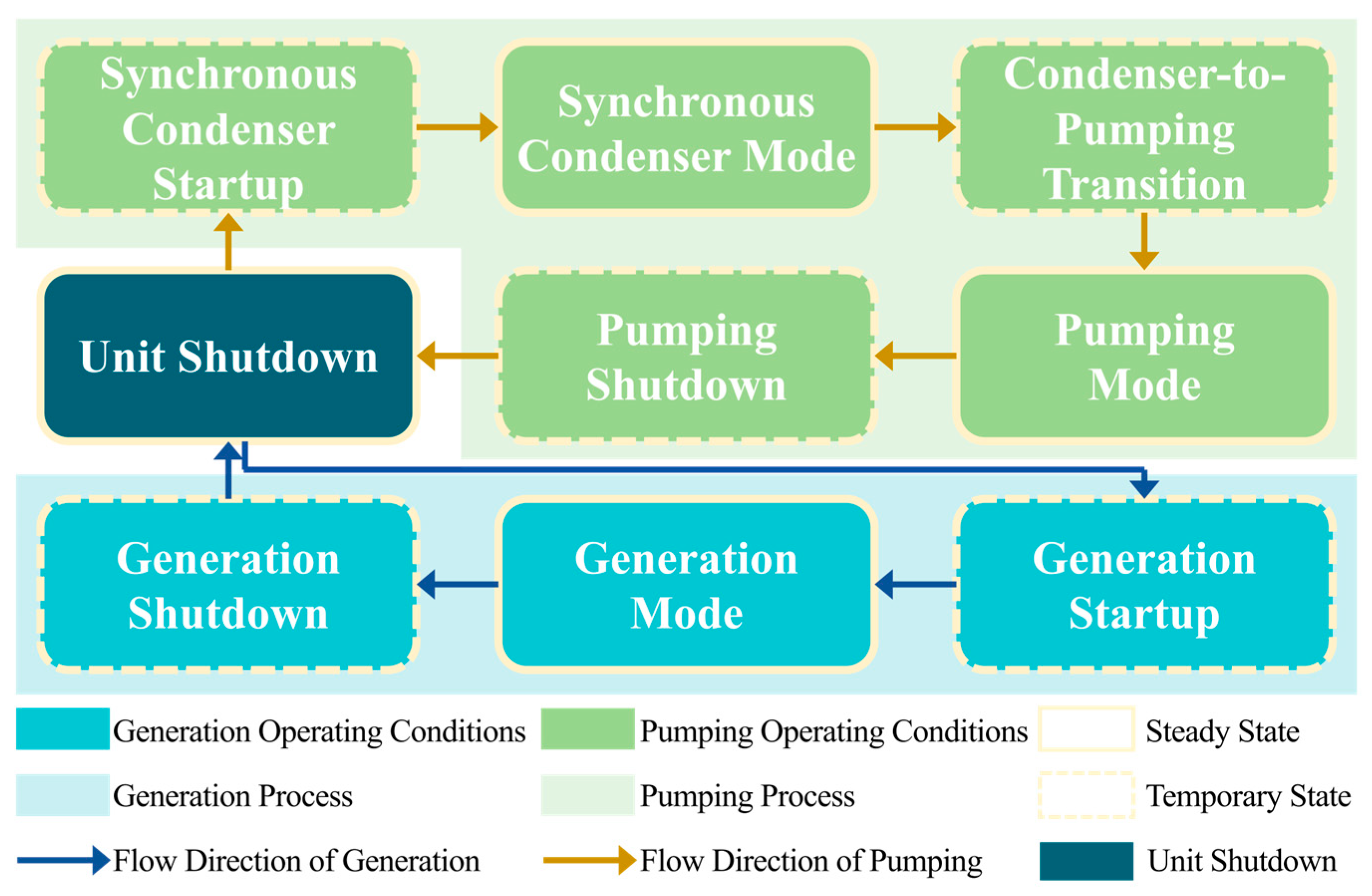
In practical operation, the pumped storage unit primarily functions in two main modes: pumping and generation. During generation, the unit starts from a shutdown state, enters a transitional phase known as generation startup, and then reaches the steady-state generation condition. In this stage, the unit converts the potential energy of water stored in the upper reservoir into electrical energy to support the power grid. Once the generation task is completed, the unit transitions through a generation shutdown process and eventually returns to the shutdown state. During the pumping stage, the unit also starts from the shutdown state and enters the pumping synchronous condenser startup phase, transitioning into the pumping synchronous condenser mode. It then passes through a transitional mode called the pumping-to-synchronous-condenser switch, during which the unit alternates between pumping and condenser states. Once in the pumping condition, the unit converts electrical energy into mechanical energy to pump water from the lower reservoir back to the upper reservoir, thereby storing energy. After completing the pumping task, the unit undergoes the pumping shutdown process and finally returns to the shutdown state.
This study defines nine operating conditions for the pumped storage unit, as shown in Figure 5. Among them, there are four steady-state conditions: unit shutdown, generation mode, pumping mode, and synchronous condenser mode. The other five are transitional states: generation startup, synchronous condenser startup, pumping shutdown, generation shutdown, and condenser-to-pumping transition.

2.2.2. Data Collection

The data used in this study were collected from the sound signals of Unit 2 at the Putian Xianyou Pumped Storage Power Station between 4 July and 12 July 2024. The sound signals were recorded using a microphone installed on a wall near the turbine in the machine hall, approximately 1.5 m above the floor. The microphone was oriented towards the turbine to capture mechanical impacts and fluid disturbances generated via components such as the pump-turbine and guide vanes. A RØDE VideoMic Me-C (Røde Microphones, Sydney, Australia) digital microphone was used, with a frequency response of 20 Hz to 20 kHz, a sampling rate of 48 kHz, and a signal-to-noise ratio of 74.5 dB. The microphone includes a built-in analog-to-digital converter and outputs high-fidelity digital audio at 48 kHz/16-bit. It was connected via USB-C to an RK3399 embedded board, which transmitted the data to a backend server in real time through a network switch. Each audio segment was 5 s long and saved in FLAC format to preserve waveform fidelity. During the data collection period, the unit operated on a typical schedule of power generation during the day and pumping at night. The dataset includes more than 10 complete cycles of pumping and shutdown, providing sufficient samples for model training and condition classification.
The dataset contains 58,798 samples for steady-state conditions, which have abundant data and highly similar features. In contrast, transitional states are represented by 1382 samples, characterized by fewer data but more complex features. To balance the class distribution and speed up training, the steady-state samples were randomly downsampled to 500 per class, while all transitional samples were retained. This resulted in a final dataset of 3413 samples. The sample distribution for each condition is detailed in Table 2. Since the number of Mel spectrogram samples remains unbalanced, class weight coefficients will be introduced during training to adjust for the disproportionate influence of categories with more samples. The dataset is split into 70% training and 30% testing sets.

3. Results

3.1. Frequency-Domain Feature Analysis

3.1.1. Data Preprocessing

The collected FLAC-format signals were first decoded to recover the time-domain waveforms. Then, a short-time Fourier transform (STFT) was applied for spectral analysis. This process divides the time-domain signal into multiple short windows, and a Fourier transform is performed on each window to obtain the frequency distribution over time. In the experiment, a 1024-point Hamming window was used for framing, with a frame shift of 512 points. Figure 6 shows the spectrograms corresponding to nine operating conditions. Noticeable differences can be seen among the conditions in terms of dominant frequency positions, frequency energy distribution, and amplitude characteristics.
The frequency spectra of steady-state conditions are stable with clear dominant frequencies. Specifically, the shutdown condition has a dominant frequency concentrated around 75 Hz, with spectral energy mainly distributed in the low-frequency range. The overall signal strength is low, with peak values not exceeding 700, reflecting weak noise output when the equipment is stationary or in a low-speed buffering state. The generation condition displays a stable periodic vibration pattern, with a dominant frequency at 100 Hz and multiple sub-peaks at harmonic frequencies such as 200 Hz and 300 Hz. The signal strength is significantly enhanced, with peaks reaching approximately 25,000. The pumping condition shows dominant frequencies at 100 Hz, 200 Hz, and 300 Hz, with dense signal energy and peak values up to 30,000, representing a typical high-energy, high-frequency operating state. In contrast, the pumping reactive power adjustment condition shifts its dominant frequency to 200 Hz and exhibits more pronounced frequency components near 400 Hz. Its overall spectral structure is smoother, with peak values around 20,000, indicating a relatively stable but slightly lower energy operating state.
Compared to steady states, transient conditions feature more abrupt frequency changes and energy fluctuations, resulting in more complex and unstable spectral structures. During the generation startup phase, frequency components mainly distribute between 100 and 300 Hz, with peak values around 7000, indicating that the unit is gradually transitioning from rest to an active vibration stage. The dominant frequency during generation shutdown shifts down to 50 Hz, with an overall spectral energy decrease and peaks maintaining around 7000, reflecting the energy decay trend at the end of operation. The pumping reactive power startup phase has a dominant frequency at 300 Hz, with signal peaks around 12,500, and it contains frequency components near 100 Hz and 600 Hz, demonstrating multimodal vibration characteristics during system startup. The synchronous condenser-to-pumping transition condition has a dominant frequency at 200 Hz with peak values reaching 30,000, where spectral energy is highly concentrated, and secondary frequency components spread in the low-frequency range, typical of a dynamic switching state. During a pumping shutdown, the dominant frequency is around 100 Hz, with peaks also reaching 30,000. Energy remains present at 200 Hz and 300 Hz, indicating that although the unit decelerates during shutdown, strong low-frequency mechanical vibrations persist. Overall, the spectral characteristics of transient conditions are more complex and difficult to model, representing a key challenge for accurate condition identification.
In summary, steady-state conditions feature regular spectral structures and clear dominant frequencies, making them easier to model and identify. Transient conditions, with their more complex spectra and pronounced nonlinear features, pose significant challenges to the performance of subsequent recognition models.

3.1.2. Mel Spectrogram Comparison

In this study, the collected raw audio signals are preprocessed and converted into Mel spectrograms for subsequent feature extraction and model input. The Mel spectrogram is a two-dimensional representation that preserves both time and frequency information, offering excellent time–frequency resolution. It is especially effective in modeling non-stationary signals and is widely used in speech recognition and acoustic monitoring applications.
The specific processing flow is shown in Figure 2. First, each 5 s audio segment undergoes a short-time Fourier transform (STFT) to convert the signal from the time domain to the frequency domain, obtaining the spectral distribution within each time window. Then, the spectrogram is passed through a Mel filter bank, which maps the linear frequency axis to the Mel scale based on human auditory perception. This mapping retains the main structural frequency features while compressing redundant information. Next, the Mel energy is logarithmically transformed to produce the final Log–Mel spectrogram, which serves as the input to the deep neural network model.
In this study, the Mel spectrogram uses 128 filter channels, with a window length of 1024 points and a frame shift of 512 points, balancing the time–frequency resolution. Figure 7 illustrates the Mel spectrograms for nine operating conditions, where stable-state conditions exhibit stable energy distribution and clear structures, while transient conditions show frequency jumps and uneven energy characteristics.
Under steady-state conditions, the Mel spectrograms exhibit uniform textures and stable harmonic structures. Energy is concentrated in specific frequency bands and varies smoothly over time, with minimal fluctuations in frequency and amplitude. This reflects the stability and periodicity of the unit’s operating state. In Figure 7b, the generation mode shows distinct harmonic peaks at around 100 Hz, 200 Hz, and 300 Hz, with dense energy distribution in the 0–512 Hz range, indicating richer low-frequency components. In Figure 7f, the pumping mode presents strong energy concentration with coarser spectral textures, and the low-frequency distribution is less uniform compared to the generation mode. In Figure 7h, the synchronous condenser mode shifts the main frequencies to around 200 Hz and 400 Hz, with a smoother spectral structure, suggesting stable operation under a relatively lower energy state. In contrast, Figure 7d shows the shutdown mode with weak energy and a flat spectral structure, mainly in the low-frequency range, which is consistent with low-speed or idle conditions.
Under transient conditions, the spectrograms become more complex, showing abrupt frequency changes and unstable energy distribution. In Figure 7a, during the startup of generation mode, spectral energy gradually increases between 100–300 Hz, and a distinct energy band appears near 512 Hz. Some spectral textures are also visible in higher-frequency regions, indicating a transition from idle to active operation. Figure 7c,e,g representing shutdown of generation, startup of pumping, and shutdown of pumping, respectively, all show prominent energy bands near 600 Hz. This may suggest a resonance or inherent vibration mode during the start-stop processes. Specifically, Figure 7c shows a downward shift in spectral energy, Figure 7e reflects rapid high-frequency excitation during startup, and Figure 7g retains strong high-frequency components even in the deceleration phase. Figure 7i, corresponding to the transition from condenser to pumping, exhibits the most complex spectrogram with three clear energy bands spanning from low to mid-high frequencies. This indicates multi-mode vibration behavior under high-energy dynamic switching. These transient spectrograms often feature vertical energy stripes and sudden frequency bands, which provide critical temporal information for analyzing state transitions and detecting anomalies.

3.2. Analysis of Model Results

This study utilizes acoustic signal data collected from pumped storage power plant units to develop a classification model based on a cascaded structure combining CNN and MHA-LSTM for operating condition recognition. The trained model is evaluated on a test dataset by plotting the confusion matrix and calculating accuracy, recall, and F1 score to analyze its performance.

3.2.1. CNN Model Results

In the preliminary classification stage, the CNN model achieved an overall accuracy of 94% on the entire test dataset consisting of 1028 samples, indicating strong overall classification performance, as shown in Table 3 and Figure 8. The CNN demonstrated robust recognition ability for steady-state categories, with F1 scores exceeding 0.96. For instance, the “Unit Shutdown” category contained 150 samples, all of which were correctly classified, achieving 100% accuracy. In the “Generation Mode” category, only one misclassification occurred among 149 samples, resulting in an F1 score above 0.96, indicating very stable performance. The “Pumping Mode” and “Synchronous Condenser Mode” also showed good results, with both precision and a recall above 0.95, reflecting strong generalization and discrimination capabilities for these conditions. The “Shutdown Class II” category, consisting of 218 samples, maintained a high recognition level with a precision of 0.96 and a recall of 0.92, although a small portion of true “Shutdown Class II” samples were still misclassified.
However, CNN’s performance in identifying dynamic startup and transitional states was relatively limited. For example, the “Condenser-to-Pumping Transition” category had a precision of 0.89, the recall dropped to 0.78, and an F1 score of 0.83, indicating room for improvement in recognizing this transitional state. For the “Generation Startup” and “Synchronous Condenser Startup” categories, precision values were 0.75 and 0.81, respectively. This suggests a relatively high number of false positives, where samples from other categories were incorrectly classified as these two. The recall rates were also low for these categories, further demonstrating the model’s difficulty in accurately identifying these samples.

3.2.2. MHA-LSTM Model Results

The MHA-LSTM model performed well in the classification task, achieving an overall prediction accuracy of 94%. As shown in Figure 9 and Table 4, for the generation shutdown category, the model correctly predicted 133 out of 141 samples, with both recall and F1 score reaching 95%. It indicates accurate identification of the majority of samples in this category. For the pumping shutdown category, precision and recall were both 91%. Among 81 pumping shutdown samples, 74 were correctly classified, resulting in recall and F1 scores of 91%, slightly lower than those for the generation shutdown category. This difference mainly arises from seven false negatives in the pumping shutdown category and eight generation shutdown samples being misclassified as pumping shutdown. Such performance discrepancies may be attributed to imbalanced data distribution, where the limited sample size for the smaller category restricts the model’s ability to fully learn its features.

3.2.3. CNN+MHA-LSTM Model Results

The performance of the CNN+MHA-LSTM condition recognition model was evaluated using the test set, achieving an overall accuracy of 92.22%. Table 5 lists the prediction accuracy metrics for each operational condition, while Figure 10 presents the confusion matrix of the model on the test data. Overall, the model demonstrated exceptional performance in identifying typical steady-state conditions. Specifically, the precision for the “Shutdown” and “Generation Mode” categories reached 0.99 and 0.98, with recall rates of 1.00 and 0.97, respectively, indicating the model’s stable and accurate recognition of the most common operating states. Furthermore, steady-state conditions such as “Pumping Mode,” “Synchronous Condenser Mode,” and “Pumping Shutdown” also achieved precision above 0.86. The F1 scores for both “Pumping Mode” and “Synchronous Condenser Mode” were 0.96, reflecting consistent and reliable performance.
Regarding transient conditions, the model exhibited moderate discriminative ability. For example, the F1 scores for “Generation Startup” and “Synchronous Condenser Startup” were 0.79 and 0.83, respectively. Although slightly lower than those of steady-state conditions, these results remain within acceptable limits. These transient states typically involve rapid transitions and significant changes in audio signals, posing challenges for the model. The “Synchronous Condenser to Pumping Transition,” one of the most dynamic transitional conditions, showed relatively complex recognition, with an F1 score of 0.83 and a recall rate of 0.78. According to the confusion matrix, this category was primarily misclassified as the adjacent “Pumping Mode” or “Synchronous Condenser Mode,” likely due to blurred condition boundaries and continuous transitions in acoustic features, which introduce uncertainty in boundary delineation by the model.

3.3. Comparative Evaluation of Models

This study selected four models for comparison to comprehensively evaluate their performance in the hydropower unit condition classification task: CNN, LSTM, GRU, and the proposed cascaded CNN+MHA-LSTM model. As shown in Table 6 and Figure 11, significant differences are observed among the four models in terms of accuracy, precision, recall, and F1 score.
It is evident from the table that the standalone CNN model performs relatively poorly across all four metrics, primarily due to its inability to effectively capture temporal dependencies within the sequential data. Both LSTM and GRU are recurrent neural network-based models, showing clear advantages in modeling time-series features. Compared to CNN, they improve classification accuracy by nearly 20%, with GRU performing slightly better than LSTM. Notably, the proposed CNN+MHA-LSTM cascaded model achieves significant improvements across all evaluation metrics. It reaches an overall accuracy of 92.22% and an F1 score of 92.17%. This represents an approximately 14% improvement in accuracy compared to the GRU model. This performance gain can be attributed to the architectural design that leverages the strengths of multiple models: the initial CNN layers effectively extract spatial local features from the input images, while the subsequent MHA+LSTM layers simultaneously model temporal dependencies and enhance attention to critical time segments. This combination of local time–frequency information and global temporal dependencies substantially boosts classification performance.

4. Conclusions and Discussion

This study proposes a two-stage cascaded classification framework combining CNN and MHA-LSTM to address the challenge of complex and variable operating condition recognition in pumped storage power plants. In the first stage, the CNN model performs preliminary classification to rapidly identify common steady-state conditions, as well as the difficult-to-distinguish “Shutdown Class II” samples. In the second stage, the MHA-LSTM model conducts fine-grained classification on these samples, enhancing the discrimination between “Generation Shutdown” and “Pumping Shutdown” conditions through sequential modeling and attention mechanisms. The cascaded framework achieves functional complementarity and hierarchical division of labor between the two stages by integrating both time–frequency features and temporal dependencies.
The proposed model achieved an overall classification accuracy of 92.22% in the task of operating condition recognition. The CNN module effectively extracted multi-scale spatial features of sound signals through its convolutional architecture, achieving F1 scores above 0.96 in classifying steady-state conditions such as unit shutdown, generation, and pumping. The MHA-LSTM component successfully captured the temporal dependencies among different operating conditions, showing particularly strong performance in the prediction of “Generation Shutdown” and “Pumping Shutdown” categories, with F1 scores of 0.95 and 0.91, respectively. The model enhanced its ability to model long-range dependencies and improved classification performance in cases with ambiguous class boundaries by MHA-LSTM. The MHA-LSTM module effectively focused on discriminative time segments in the signals, enabling accurate distinction between complex transition conditions such as generation shutdown and pumping shutdown. This addressed the limitations of traditional models, which often suffer from low accuracy and high misclassification rates in such scenarios. MHA demonstrated superior classification stability and generalization capability throughout the study, offering more precise support for fine-grained condition recognition in pumped storage units. Finally, the cascaded CNN + MHA-LSTM model further enhanced recognition performance for startup and transition conditions, achieving comprehensive modeling and classification across both steady and dynamic operating states.
The experimental results demonstrate that the proposed cascaded classification model outperforms traditional single models such as CNN, LSTM, and GRU in the task of operating condition recognition. Compared with individual models, the proposed method achieves an overall accuracy improvement ranging from 13.7% to 34.7%, and an increase of over 20% in F1 score. Notably, the model performs significantly better in identifying dynamic and transitional operating conditions. These results indicate that the CNN + MHA-LSTM hybrid architecture possesses stronger capabilities in feature extraction and temporal modeling, making it especially suitable for complex, variable, and boundary-blurred condition classification tasks. Although some previous studies have explored acoustic feature analysis in the context of mechanical fault diagnosis, there remains a lack of unified and high-precision modeling approaches for fine-grained acoustic condition recognition in pumped storage units. The cascaded strategy and model architecture proposed in this study provide a feasible solution to this problem and exhibit strong generalization and scalability potential.
This study addresses the gap in noise-based recognition technologies for pumped storage equipment by optimizing the model architecture. The proposed approach provides both theoretical foundations and modeling support for unit condition monitoring based on acoustic signals, which holds significant practical importance for ensuring the secure operation of power system load regulation and frequency control. In the future, this method can be extended to multi-source data fusion, such as incorporating signals from vibration, temperature, and current, to enable more accurate condition prediction and status monitoring. For instance, combining acoustic data with temperature measurements could help detect early-stage faults such as bearing overheating or lubrication anomalies [28]. Furthermore, data-driven approaches could be combined with the underlying generation mechanisms of vibration and noise—such as hydraulic excitation and electromagnetic effects—for a more interpretable and physically grounded analysis [29]. This would offer robust support for the health management and predictive maintenance of power station equipment.

Author Contributions

Conceptualization, L.K. and J.L.; methodology, Z.Z., W.L. and J.L.; software, N.H.; validation, H.Z. and X.Z.; formal analysis, Z.Z.; investigation, Y.L.; resources, H.Z.; data curation, J.W.; writing—original draft preparation, Z.Z., W.L. and J.L.; writing—review and editing, L.K., Z.Z. and W.L.; visualization, Z.Z.; supervision, N.H.; project administration, H.Z.; funding acquisition, N.H. and J.L. All authors have read and agreed to the published version of the manuscript.

Funding

This research was funded by the Science and Technology Project of State Grid Xin Yuan Company Limited (grant number SGXYKJ-2023-027) and the Science and Technology Service Network Plan (STS) (grant numbers 2022T3029).

Data Availability Statement

The original contributions presented in the study are included in the article; further inquiries can be directed to the corresponding author.

Conflicts of Interest

Authors Linghua Kong, Nan Hu, Hongyong Zheng, Xulei Zhou, and Jian Wang were employed by the company Fujian Xianyou Pumped Storage Power Co., Ltd. Authors Yang Lu was employed by the company Unisound AI Technology Co., Ltd. The remaining authors declare that the research was conducted in the absence of any commercial or financial relationships that could be construed as a potential conflict of interest.

References

  1. Bogdanov, D.; Ram, M.; Aghahosseini, A.; Gulagi, A.; Oyewo, A.S.; Child, M.; Caldera, U.; Sadovskaia, K.; Farfan, J.; Barbosa, L.D.S.N.S. Low-Cost Renewable Electricity as the Key Driver of the Global Energy Transition towards Sustainability. Energy 2021, 227, 120467. [Google Scholar] [CrossRef]
  2. Wen, F.; Lu, G.; Huang, J. Integrated Energy System towards Carbon Peak and Neutrality Targets. J. Glob. Energy Interconnect. 2022, 5, 116–117. [Google Scholar]
  3. China to Vigorously Develop Wind and Solar Power in the Next Decade. Available online: https://www.gov.cn/xinwen/2020-12/15/content_5569658.htm (accessed on 7 July 2025).
  4. Chen, H.; Li, H.; Xu, Y.; Chen, M.; Wang, L.; Dai, X.; Xu, D.; Tang, X.; Li, X.; Hu, Y. Research Progress on Energy Storage Technologies of China in 2022. Energy Storage Sci. Technol. 2023, 12, 1516. [Google Scholar]
  5. Zhang, W. Study on Hybrid Intelligent Fault Diagnosis and State Tendency Prediction for Hydroelectric Generator Units. Master’s Thesis, Huazhong University of Science and Technology, Wuhan, China, 2019. [Google Scholar]
  6. Wei, B.; Ji, C. Study on Rotor Operation Stability of High-Speed Large-Capacity Generator-Motor: The Accident of Rotor Pole in Huizhou Pumped-Storage Power Station. Shuili Fadian/Water Power 2010, 36, 57–60. [Google Scholar]
  7. Velasquez, V.; Flores, W. Machine learning approach for predictive maintenance in hydroelectric power plants. In Proceedings of the 2022 IEEE Biennial Congress of Argentina (ARGENCON), Buenos Aires, Argentina, 7–9 September 2022; pp. 1–6. [Google Scholar]
  8. Wang, H.; Ma, Z. Regulation Characteristics and Load Optimization of Pump-Turbine in Variable-Speed Operation. Energies 2021, 14, 8484. [Google Scholar] [CrossRef]
  9. Yang, K.; OuYang, G.; Ye, L. Research upon fault diagnosis expert system based on fuzzy neural network. In Proceedings of the 2009 WASE International Conference on Information Engineering, Taiyuan, China, 10–11 July 2009; pp. 410–413. [Google Scholar]
  10. Feng, Z.; Liang, M.; Chu, F. Recent Advances in Time–Frequency Analysis Methods for Machinery Fault Diagnosis: A Review with Application Examples. Mech. Syst. Signal Process. 2013, 38, 165–205. [Google Scholar] [CrossRef]
  11. Mechefske, C.K. Objective Machinery Fault Diagnosis Using Fuzzy Logic. Mech. Syst. Signal Process. 1998, 12, 855–862. [Google Scholar] [CrossRef]
  12. Wu, J.; Wang, Y.; Bai, M.R. Development of an Expert System for Fault Diagnosis in Scooter Engine Platform Using Fuzzy-Logic Inference. Expert Syst. Appl. 2007, 33, 1063–1075. [Google Scholar] [CrossRef]
  13. Hui, K.H.; Hee, L.M.; Leong, M.S.; Abdelrhman, A.M. Time-Frequency Signal Analysis in Machinery Fault Diagnosis: Review. Adv. Mater. Res. 2014, 845, 41–45. [Google Scholar] [CrossRef]
  14. Singh, G.K.; Ahmed Saleh Al Kazzaz, S.A. Induction Machine Drive Condition Monitoring and Diagnostic Research—A Survey. Electr. Power Syst. Res. 2003, 64, 145–158. [Google Scholar] [CrossRef]
  15. Yu, L.; Yao, X.; Yang, J.; Li, C. Gear Fault Diagnosis through Vibration and Acoustic Signal Combination Based on Convolutional Neural Network. Information 2020, 11, 266. [Google Scholar] [CrossRef]
  16. Ball, A.D.; Gu, F.; Li, W. The condition monitoring of diesel engines using acoustic measurements part 2: Fault detection and diagnosis. In Proceedings of the SAE 2000 World Congress, Detroit, MI, USA, 6–9 March 2000; SAE International: Warrendale, PA, USA, 2000; pp. 1–10. [Google Scholar]
  17. Zhu, Z.; Peng, G.; Chen, Y.; Gao, H. A Convolutional Neural Network Based on a Capsule Network with Strong Generalization for Bearing Fault Diagnosis. Neurocomputing 2019, 323, 62–75. [Google Scholar] [CrossRef]
  18. Kumar, A.; Gandhi, C.; Zhou, Y.; Kumar, R.; Xiang, J. Improved Deep Convolution Neural Network (CNN) for the Identification of Defects in the Centrifugal Pump Using Acoustic Images. Appl. Acoust. 2020, 167, 107399. [Google Scholar] [CrossRef]
  19. Hochreiter, S.; Schmidhuber, J. Long Short-Term Memory. Neural Comput. 1997, 9, 1735–1780. [Google Scholar] [CrossRef]
  20. Dao, F.; Zeng, Y.; Qian, J. Fault Diagnosis of Hydro-Turbine via the Incorporation of Bayesian Algorithm Optimized CNN-LSTM Neural Network. Energy 2024, 290, 130326. [Google Scholar] [CrossRef]
  21. Zhou, J.; Shan, Y.; Liu, J.; Xu, Y.; Zheng, Y. Degradation Tendency Prediction for Pumped Storage Unit Based on Integrated Degradation Index Construction and Hybrid CNN-LSTM Model. Sensors 2020, 20, 4277. [Google Scholar] [CrossRef] [PubMed]
  22. Niu, Z.; Zhong, G.; Yu, H. A Review on the Attention Mechanism of Deep Learning. Neurocomputing 2021, 452, 48–62. [Google Scholar] [CrossRef]
  23. Zhang, W.; Zhang, T.; Jia, M.; Cai, J. Remaining Useful Life Prediction of Motor Bearings Using Multi-Sensor Fusion and MHA-LSTM. Yiqi Yibiao Xuebao (Chin. J. Sci. Instrum.) 2024, 45, 84–93. [Google Scholar]
  24. Fan, X.; Meng, F.; Deng, J.; Semnani, A.; Zhao, P.; Zhang, Q. Transformative Reconstruction of Missing Acoustic Well Logs Using Multi-Head Self-Attention BiRNNs. Geoenergy Sci. Eng. 2025, 245, 213513. [Google Scholar] [CrossRef]
  25. Yang, Z.; Li, C.; Wang, X.; Chen, H. Intelligent Fault Monitoring and Diagnosis of Tunnel Fans Using a Hierarchical Cascade Forest. ISA Trans. 2023, 136, 442–454. [Google Scholar] [CrossRef]
  26. Zhang, Y.; Xu, T.; Chen, C.; Wang, G.; Zhang, Z.; Xiao, T. A Hierarchical Method Based on Improved Deep Forest and Case-Based Reasoning for Railway Turnout Fault Diagnosis. Eng. Fail. Anal. 2021, 127, 105446. [Google Scholar] [CrossRef]
  27. LeCun, Y.; Bottou, L.; Bengio, Y.; Haffner, P. Gradient-based learning applied to document recognition. Proc. IEEE 2002, 86, 2278–2324. [Google Scholar] [CrossRef]
  28. Zhao, Y.; Wang, X.; Han, S.; Lin, J.; Han, Q. Fault Diagnosis for Abnormal Wear of Rolling Element Bearing Fusing Oil Debris Monitoring. Sensors 2023, 23, 3402. [Google Scholar] [CrossRef]
  29. Zhang, H.; Li, K.; Liu, T.; Liu, Y.; Hu, J.; Zuo, Q.; Jiang, L. Analysis the Composition of Hydraulic Radial Force on Centrifugal Pump Impeller: A Data-Centric Approach Based on CFD Datasets. Appl. Sci. 2025, 15, 7597. [Google Scholar] [CrossRef]
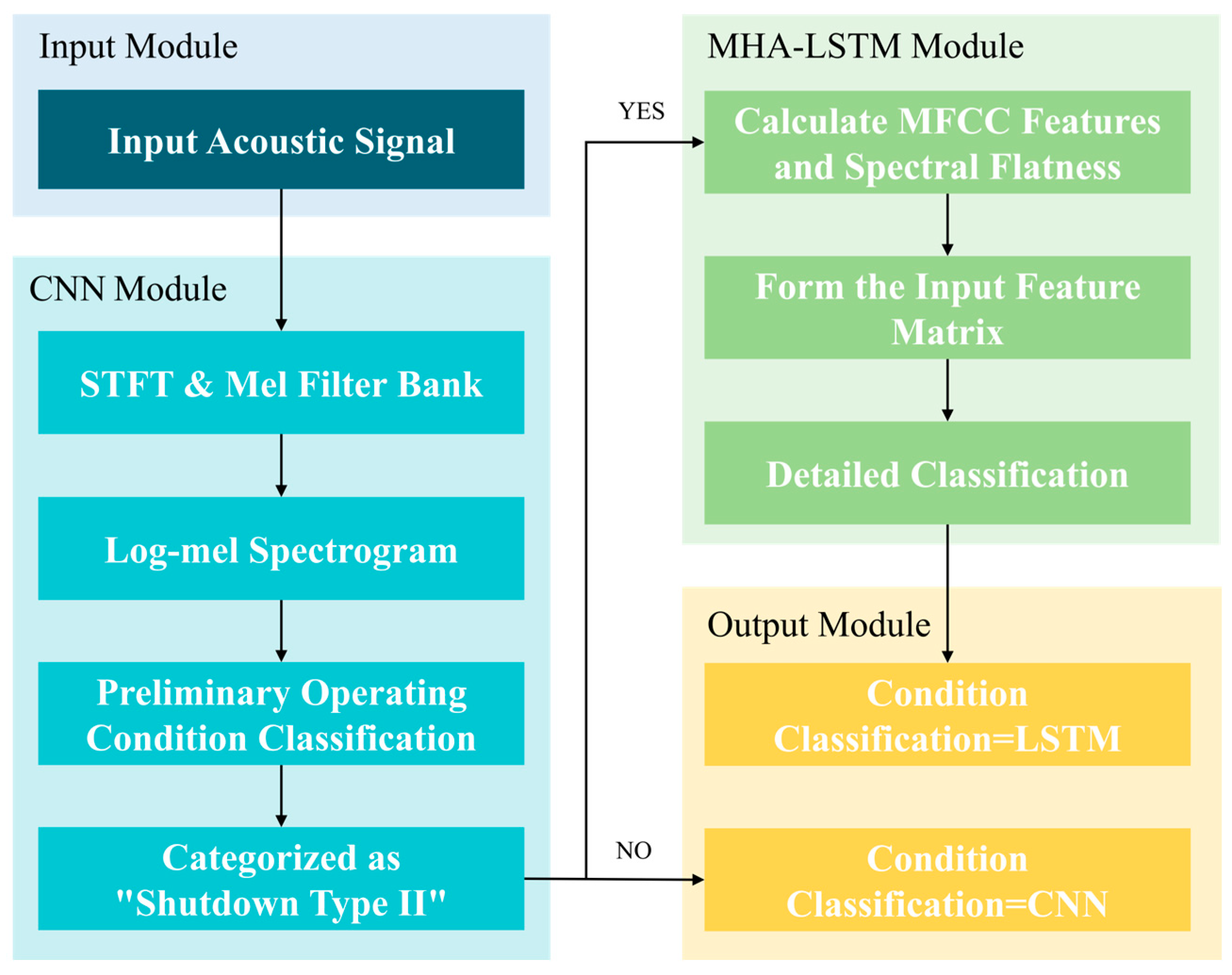
Figure 1. Research framework.
Energies 18 04269 g001
Figure 2. The classical structure of a CNN.
Energies 18 04269 g002
Figure 3. The internal structure of LSTM.
Energies 18 04269 g003
Figure 4. The structure of MHA-LSTM.
Energies 18 04269 g004
Figure 5. Operating condition transition diagram.
Energies 18 04269 g005
Figure 6. Frequency spectra of different operating conditions: (a) unit shutdown, (b) generation mode, (c) synchronous condenser, (d) pumping mode, (e) generation startup, (f) generation shutdown, (g) pumping startup, (h) condenser-to-pumping transition, (i) pumping shutdown.
Energies 18 04269 g006
Figure 7. Sound spectrograms under different operating conditions of the pumped storage unit: (a) generation startup, (b) generation mode, (c) generation shutdown, (d) unit shutdown, (e) synchronous condenser startup, (f) pumping mode, (g) pumping shutdown, (h) synchronous condenser, (i) condenser-to-pumping transition.
Energies 18 04269 g007
Figure 8. Confusion matrix of the CNN model.
Energies 18 04269 g008
Figure 9. Confusion matrix of the MHA-LSTM Model.
Energies 18 04269 g009
Figure 10. Confusion matrix of the CNN+MHA-LSTM Model.
Energies 18 04269 g010
Figure 11. Evaluation metrics of four models on the test set.
Energies 18 04269 g011
Table 1. Structure parameters in each layer of CNN.
LayerKernel SizeStrideNumber of ChannelsOutput Size
Conv2D3 × 31 × 132222 × 222 × 32
MaxPooling2D2 × 22 × 232111 × 111 × 32
Conv2D3 × 31 × 164109 × 109 × 64
MaxPooling2D2 × 22 × 26454 × 54 × 64
Conv2D3 × 31 × 112852 × 52 × 128
MaxPooling2D2 × 22 × 212826 × 26 × 128
Flatten///26 × 26 × 128
Dense//128128
Dropout///128
Dense (Softmax)//88
Table 2. Sample size for each operating condition of the unit.
Condition TypeTotal SamplesTraining SetTesting Set
unit shutdown500350150
generation mode500350150
generation startup17712453
generation shutdown470329141
pumping shutdown26718780
pumping mode500350150
Synchronous Condenser startup30121190
condenser-to-pumping transition16711750
Table 3. Prediction accuracy, recall, and F1 score of the CNN model.
ClassificationPrecisionRecallF1 Score
Unit Shutdown0.991.000.99
Shutdown Class II0.960.920.94
Generation Mode0.970.990.98
Generation Startup0.740.850.79
Pumping Mode0.950.970.96
Synchronous Condenser Mode0.950.960.96
Synchronous Condenser Startup0.850.810.83
Condenser-to-Pumping Transition0.890.780.83
Table 4. Prediction accuracy, recall, and F1 score of the MHA-LSTM Model.
ClassificationPredictionRecall
generation shutdown0.950.95
pumping shutdown0.910.91
Table 5. Prediction accuracy, recall, and F1 score of the CNN+MHA-LSTM Model.
ClassificationPrecisionRecallF1 Score
Unit Shutdown0.991.000.99
Generation Shutdown0.910.840.87
Generation Mode0.970.990.98
Generation Startup0.740.850.79
Pumping Shutdown0.860.880.87
Pumping Mode0.950.970.96
Synchronous Condenser Mode0.950.960.96
Synchronous Condenser Startup0.850.810.83
Condenser-to-Pumping Transition0.890.780.83
Table 6. Evaluation metrics of four models on the test set.
Classification
Model
Accuracy
(%)
Precision
(%)
CNN57.5655.45
LSTM76.4666.65
GRU78.5069.81
CNN+MHA-LSTM92.2292.26
Disclaimer/Publisher’s Note: The statements, opinions and data contained in all publications are solely those of the individual author(s) and contributor(s) and not of MDPI and/or the editor(s). MDPI and/or the editor(s) disclaim responsibility for any injury to people or property resulting from any ideas, methods, instructions or products referred to in the content.