Abstract
As the global carbon neutrality process accelerates, the proportion of distributed power sources such as wind power and photovoltaic power continues to increase. This transformation, while promoting the development of clean energy, also brings about the issue of new energy consumption. As wind and solar distributed generation rapidly expands into modern power grids, consumption issues become increasingly prominent. In this paper, a robust optimal scheduling method considering multiple uncertainties is proposed for community microgrids containing multiple renewable energy sources based on potential games. Firstly, the flexible loads of community microgrids are quantitatively classified into four categories, namely critical base loads, shiftable loads, power-adjustable loads, and dispersible loads, and a stochastic model is established for the wind power and load power; secondly, the user’s comprehensive electricity consumption satisfaction is included in the operator’s scheduling considerations, and the user’s demand is quantified by constructing a comprehensive satisfaction function that includes comfort indicators and economic indicators. Further, the flexible load-response expectation uncertainty and renewable generation uncertainty model are used to establish a robust optimization uncertainty set. This set portrays the worst-case scenario. Based on this, a two-stage robust optimization framework is designed: with the dual objectives of minimizing operator cost and maximizing user satisfaction, a potential game model is introduced to achieve a Nash equilibrium between the interests of the operator and the users, and solved by a column and constraint generation algorithm. Finally, the rationality and effectiveness of the proposed method are verified through examples, and the results show that after optimization, the cost dropped from CNY 2843.5 to CNY 1730.8, a reduction of 39.1%, but the user satisfaction with electricity usage increased to over 98%.
1. Introduction
Microgrids act as a key bridge between distributed resources and the power grid, play a critical role in improving renewable energy integration, and are an important component in the construction of new power systems. At the same time, as the proportion of renewable energy continues to increase, the reliability and stability of the new type of power system is becoming more and more prominent, and there is a need to mobilize a variety of flexible resources to participate in the operation and control of the system. More and more community users are installing photovoltaic panels on the roof. Thus, community users are no longer the traditional single power consumers; they are gradually experiencing a “producer–consumer” role change. And with wind and other renewable energy being distributed, and massive and diversified access to the grid, the grid’s operation and scheduling has brought new challenges. Microgrids are an effective method for applying multi-type distributed power supply and a functional interface between distributed sources and the power grid, with broad development prospects and diversified application scenarios [1,2,3].
In the initial research of microgrid operation optimization, it mainly focuses on the optimization of the single objective of economy or reliability in order to achieve the purpose of reducing the user’s electricity bill or improving the reliability of electricity consumption. For example, one study [4] constructed a cooperative game model of a multi-microgrid system with the optimization objective of improving the economic efficiency of the multi-microgrid system and proposed a benefit-compromise algorithm to solve the operation optimization problem of the multi-microgrid system, while another study [5] took into account the uncertainty of the photovoltaic (PV) generation output and adopted a deep reinforcement-learning algorithm with the objective of minimizing the operating cost of the microgrid, which in turn improves the economic performance of the microgrid system. Reference [6] proposed a model-based predictive control algorithm for managing the energy storage system in islanded operation mode with the goal of ensuring the stability of microgrid operation. References [7,8] firstly adopted a clustering method to cut down the scenarios, taking into account the integrated demand response of multiple types of loads, so as to construct a master–slave game model and realize the different interests through the optimization of trading tariffs and the coupling of the decision-making roles of microgrid purchasing and selling plans. It is the main body of the win-win situation.
The abovementioned studies are based on the premise of a 100% user demand-response rate of deterministic scenarios; in the default, the user will follow the scheduling instructions for demand-response based on the study, but in the actual operation and control process of the grid, the user will be affected by many uncertainties, leading to the user’s actual response and scheduling results failing to achieve the desired outcomes due to various uncertainties. Aiming at the above problems, Reference [9] takes the environmental awareness of users’ electricity consumption into consideration, evaluates the magnitude of the response volume by quantifying the psychological uncertainty of users’ consumption, and calculates to obtain the range of variation in users’ participation, which in turn improves the economics of microgrid scheduling. In another work from the literature [10], an adaptable method for evaluating demand-response potential through deep subdomains is introduced, harnessing the resemblance of parameter attributes to forecast how demand response may perform. Incorporating robust optimization improves resilience against uncertainty risks and increases flexibility during system dispatch operations. Game theory has many applications in the power system, used to solve the operational optimization of the power system and decision-making problems in energy trading. Reference [11] constructed a two-layer distributed optimization model, and the two-layer model constitutes a master–slave game problem. Reference [12] established a master–slave game model for distribution networks and multiple micro-networks, with the distribution network as the leader and the micro-network as the follower.
In conclusion, the existing research has the following problems that need to be solved: (1) handling unilateral uncertainty, (2) rigid response assumption, (3) absence of game equilibrium. Building on the previously discussed multi-body interest game analysis, this study centers on the coordinated management of flexible loads within community microgrids, striving to meet the electricity demands of dispatching users. To this end, a robust optimal scheduling method for unified management of microgrid flexible loads by operators is proposed. The innovation points of this paper are as follows: (1) For the first time, the potential game theory is applied to the dispatching of community-level microgrids. (2) We develop a new paradigm of robust optimization driven by response expectations. (3) Empirical verification is conducted on the feasibility of the synergy between the dual goals of “economy and comfort”. With full consideration of the uncertainties in wind and photovoltaic power generation, stochastic models are developed to refine the uncertainty set in robust optimization, targeting various types of flexible loads based on user-response expectations. In addition, a multi-objective optimization function covering the operator’s and the microgrid’s flexible loads is established. The effectiveness of the proposed optimal scheduling method is verified through a case study. This approach not only enhances the stability of grid operations but also ensures a win-win outcome for both users and operators, while maintaining microgrid users’ satisfaction with their electricity consumption.
2. Community Microgrid Operators and Flexible Load Modeling
In this study, we focus on a community microgrid operator equipped with wind, photovoltaic, and storage units—which represent the predominant share of current development. Figure 1 illustrates the overall system architecture. The operators act as intermediaries, connecting users of the community microgrid with the power grid. Among them, the aggregators have their own independent new energy power generation equipment and energy storage equipment. The community microgrid also has photovoltaic systems and energy storage systems. The operator achieves the purpose of making profits by cluster regulating the controllable loads in the community microgrid. By coordinating operations in this way, microgrid users benefit from more effective scheduling than they would achieve on their own. Managing building clusters becomes possible for an operator upon signing a load scheduling agreement; this involves accounting for the load curve, upper-level grid time-based pricing, and consumer satisfaction with their electricity use. Therefore, once the community microgrid users have an agreement with the operator, the operator can manage the dispatchable flexible loads of the building clusters at suitable times in accordance with the load curve, the higher-level grid’s time-of-use rates, and the users’ comfort in electricity usage. This approach ultimately enables the operator to gain economic benefits.
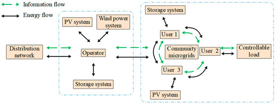
Figure 1.
Schematic diagram of system architecture.
2.1. Community Microgrid Operator Modeling
2.1.1. Photovoltaic System Model
The power generated by the operator’s PV plant can be expressed as follows:
where is the temperature coefficient of PV equipment; and are the actual operating temperature of the photovoltaic panels and the reference temperature, respectively; is the maximum output power of the photovoltaic panels under the standard conditions; and and are the actual light intensity and the reference light intensity, respectively.
A common representation for photovoltaic cell operating and maintenance costs is the following formula:
where is the O&M cost factor of the PV cell.
2.1.2. Wind Power System Model
The output power of the operator’s wind turbine can be expressed as follows:
where is the power generated by the wind turbine; is the wind utilization factor; is the air density; is the radius of the wind turbine; are the actual wind speed, the cut-in wind speed, the rated wind speed, and the cut-out wind speed, respectively; and is the maximum value of the power produced by the wind turbine.
The O&M cost of a wind turbine can be expressed as follows:
where is the O&M cost factor for wind turbines.
2.1.3. Energy Storage System Modeling
The energy storage system’s state of charge can be represented as follows:
where is the charging state of the energy storage system at time ; and are the charging and discharging power of the energy storage system at time ; is the unit time of the calculation cycle; is the charging and discharging efficiency of the energy storage system; is the rated capacity of the energy storage battery; and are the ending and starting moments of a scheduling cycle; and is the charging and discharging power of the energy storage system at time .
The O&M cost of an energy storage system can be expressed as follows:
where is the O&M cost factor per unit capacity of the energy storage system.
2.1.4. Transmission Power Between the Operator and the Distribution Grid
When the load in the community microgrid rises beyond a specific threshold, and the new energy generation by the operator, along with the stored energy, is insufficient to meet the demand, the operator procures power from the higher-level grid based on its time-of-use electricity pricing, . The power transmission from the higher-level grid is constrained by the transmission capacity of the connecting line.
where is the higher-level grid limit of power transfer for the contact line.
2.2. Community Microgrid User and Generalized Load Modeling
A community microgrid is typically marked by diverse power-consuming devices, a high load density, and relatively clustered electricity demands. Some intelligent devices must run continuously without interruption, making the reliability and quality of power supply crucial for ensuring the stable operation of networks. Based on the nature of the loads and how controllable they are, community microgrid loads can be classified into critical base loads, shiftable loads, power-adjustable loads, and dispersible loads.
2.2.1. Critical Base Load Modeling
Critical base loads are essential pieces of electrical equipment that function consistently over relatively fixed durations, including devices like pumps and lifts. Because these loads run without interruption, they are not involved in the operator’s power scheduling. We denote important base loads by .
2.2.2. Shiftable Load Modeling
Shiftable loads refer to loads whose overall duration of operation remains the same, but whose start and end times can be rearranged. Once initiated, these loads must run without interruption. Typically, they are scheduled to shift from high-price periods to off-peak times, thereby reducing energy costs. We can represent shiftable loads mathematically, as follows:
where is the initial electricity consumption at moment before the dispatch of the shiftable load; is the unit time of the calculation cycle; and is a 0–1 variable characterizing the operating state of the shiftable load at moment .
2.2.3. Power-Adjustable Load Modeling
Examples such as inverter ACs and smart electric blankets fall under adjustable loads. These devices operate without fixed power levels, enabling targeted energy reduction in specific timeframes while maintaining normal operation. They can be mathematically represented as follows:
where is the raw power of the adjustable load at the time ; is the power regulation margin of the adjustable load; is the 0–1 variable characterizing the operating state of the adjustable load at the time ; and is the unit time of the calculation cycle.
2.2.4. Dispersible Load Modeling
Dispersible loads refer to devices such as Electric Vehicle (EV) charging stations, which can flexibly arrange their electricity consumption and operating schedules within a given dispatch cycle, while maintaining a constant total energy consumption. The typical scheduling strategy for this category of loads is to shift electricity demand from high-tariff periods to lower-tariff periods (often at night). Mathematically, the dispersible load can be represented as follows:
where is the original power of the dispersible load at the time ; is the regulation coefficient of the power used by the dispersible load; is the 0–1 variable characterizing the operating state of the dispersible load at the time ; and is the unit time of the calculation cycle.
To ensure that the total electricity consumption of dispersible loads remains constant while enabling operational flexibility, the following constraints must be satisfied, derived from key principles in load management and grid optimization:
where is the total electricity consumption of the dispersible load.
2.2.5. Community Microgrid Energy Storage Modeling
New building energy storage systems’ state of charge is formulated as follows:
where is the charging state of the energy storage system at the time ; and are the energy storage system’s charging and discharging power at the time ; is the charging and discharging efficiency of the energy storage system; is the rated capacity of the energy storage battery; and is the charging and discharging amount of the energy storage in the building at the time .
The O&M cost of the new building energy storage system can be expressed as follows:
Therefore, the total load before customer-side dispatch of the community microgrid,, can be expressed as follows:
where is the power generated by the photovoltaic equipment of the new building at moment .
The total load after generalized user-side dispatch of the community microgrid can be expressed as follows:
2.2.6. Electricity Comfort Modeling
The overall satisfaction of microgrid users with their power supply is closely linked to the operator’s dispatch efficiency and profitability. If an operator focuses solely on its own interests, leading to frequent user power cuts due to cluster-level adjustments, this will erode its credibility, slow down responsiveness, and may ultimately result in the loss of scheduling capability and subsequent financial losses. Consequently, while striving for profitability, operators must regard user satisfaction with electricity consumption as an equally vital factor. The satisfaction model for electricity consumption incorporates both comfort and economic dimensions, capturing the daily power usage psychology of microgrid users.
- (1)
- Electricity comfort level
The electricity comfort indicator, , is employed to gauge the user’s comfort level throughout the electricity consumption process. It is assumed that when users follow their habitual consumption patterns without participating in demand response, their comfort level is maximized. By measuring the ratio of post-dispatch actual consumption deviation from scheduled usage, this indicator captures the extent to which user habits are modified. Mathematically, it can be expressed as follows:
- (2)
- Electricity economy consumption level
The electricity-use economics metric, , captures how much users save on electricity costs by taking part in the operator’s scheduling, measured as a fraction of their original (pre-scheduling) expenses. This metric thus reflects the economic benefits gained by users:
Therefore, the customer’s satisfaction with electricity consumption, , can be expressed as follows [13]:
where is the weight value of customer satisfaction with electricity at moment .
3. Modeling Generalized Load-Response Expectation Uncertainty
During demand response, there is often a deviation between the operator’s expected dispatch of flexible loads and the actual dispatch volume. This deviation primarily occurs because some flexible loads do not respond as planned or respond with delays. Consequently, the actual dispatch load is smaller than the planned load. This shortfall adversely affects the dispatch effectiveness and reduces the operator’s operational revenue. Therefore, this section will construct the response quantity expectation uncertainty model of three types of flexible loads, namely shiftable loads, power-adjustable loads, and dispersible loads, which are subject to power dispatch, and use it to improve the uncertainty set in the robust optimization algorithm.
3.1. Response Volume Expectations for Shiftable Loads
The uncertainty in the expectation of the shiftable load-response volume consists of many factors, as follows.
- (1)
- Dispatch volume of shiftable loads:
The amount of dispatch of shiftable loads greatly affects the scheduling results, and the larger the number of flexible loads expected to be dispatched, the greater the likelihood that microgrid users may be affected by electricity consumption, and the smaller the expectation of the shiftable loads’ response quantity will be. The dispatch quantity, , of the shiftable load can be expressed as follows:
- (2)
- Dispatch length of the shiftable loads:
The scheduling length of the shiftable load reflects the response psychology of the dispatched flexible load to some extent if the longer the time of a single dispatch of the shiftable load means that the greater the time cost of the shiftable load, the smaller the response volume expectation of the shiftable load. The scheduling time, , of the shiftable load can be expressed as follows:
where and are the start time and end time of electricity consumption of the shiftable load, respectively.
The above indicators and their weights are used in binary logistic regression [14] to construct the response expectation uncertainty function as follows:
3.2. Response Volume Expectations for Power-Adjustable Loads
Most of the power-adjustable loads are air conditioners, heating equipment, etc., and when the set temperature is reached near the time of reducing its power, the user’s body temperature will not change too much in a short period of time, so when the microgrid operator is scheduling the power-adjustable loads, the user’s power consumption habits are almost unchanged, therefore, the expectation of the response quantity of the power-adjustable loads basically presents a normal distribution according to the scheduling cycle, and the expectation of the response quantity of the power-adjustable loads can be expressed in the uncertainty model as a function of the power-adjustable loads [15]. The uncertainty model can be expressed as follows:
where and are the mean and standard deviation of the power-adjustable load-response capacity, respectively.
3.3. Response Volume Expectations for Dispersible Loads
The uncertainty of the expected dispersible load-response quantity includes the following two factors:
- (1)
- The endowment effect of dispersible load users
The endowment effect was proposed by behavioral economist Thaler. In economics, it refers to the fact that after an individual possesses a certain item, their expectations and evaluation of it will increase significantly compared to when they did not own it. The endowment effect reflects an individual’s perceptual bias in judging the value of items. Individuals tend to regard the items they already possess as endowments and pay more attention to the value of the items they already have compared to those they have not obtained. The endowment effect also influences the consumption psychology of electricity users. When aggregators conduct power dispatching for users, users will regard the right to use electricity they possess as an endowment. At this time, users will enhance their value evaluation of the right to use electricity. Therefore, the dispatching results will be affected by the endowment effect. Denote the endowment effect factor as , and the value range is [0,1].
- (2)
- The total operating duration of the dispersible load
Since the dispersible load can reasonably allocate the power consumption, as well as the time of power consumption, while keeping the total power consumption unchanged in a dispatch cycle, if the microgrid operator sets the dispatch time of the dispersible load for a longer period of time, the greater the impact on the microgrid users, and the lower the expectation of the response amount of the dispersible load is. The total operation time, , of the dispersible load can be expressed as follows:
where is the total original power consumption time of the dispersible load; and , , and are the operation time, dispatch start time, and dispatch end time of the dispersible load, respectively.
The uncertainty model for the expectation of the response quantity of the dispersible load can be expressed as follows:
4. A Two-Stage Robust Optimization Model Based on Potential Games
4.1. Definition of Potential Game
Within game theory—a framework analyzing strategic interactions and equilibria—the potential game is a critical non-cooperative variant. Its industry relevance stems from enabling tractable equilibrium solutions for complex multi-agent decision problems. The key distinction between a potential game and conventional game models lies in the existence of a potential function. This function directly reflects changes in the utility of game participants, enabling a structured analysis of their strategic adjustments.
One of the defining properties of potential games is the finite improvement property (FIP); this implies that players attain a Nash equilibrium within finite iterations, guaranteeing model convergence, where both the building cluster aggregator and individual users act based on self-interest. Specifically, the aggregator seeks to minimize operational costs, while users aim to maximize their electricity usage comfort. The potential game framework facilitates a balance between these objectives, making it a suitable approach for modeling energy management in intelligent building systems.
A potential game is formally defined as a strategic interaction framework where we have the following: for a game with a finite number of participants, if there is a function of , then for each participant, we have , and for any two of its strategies, we have . And for ,
where N is the game participant; and are the strategy space for the i-th participant and other participants; and is the income of the i-th participant.
Then, game is called a completely latent game, and function Q is called a latent function. The proof of necessity for the existence of a Nash equilibrium solution in this game is presented in Appendix A.
4.2. Robust Optimization Uncertainty Set Building
Rising integration of renewable energy sources amplifies weather-induced volatility in upper-tier grid and microgrid operations, resulting in substantial output fluctuations [16,17]. This poses substantial challenges to the resilience of the distribution grid, which includes the higher-level grid, operators, and microgrids, ensuring that the robustness of the distribution grid has thus become a critical concern. Operators implementing robust optimization strategies reserve a certain regulation margin in their operations to enhance the reliability and stability of their systems.
The uncertainty of renewable energy output and load response can be expressed as follows:
where , , and are the values of uncertainty fluctuation for microgrid operator PV, microgrid PV, and wind power, respectively; , , and are the actual values for operator PV, microgrid PV, and wind power, respectively; , , and are the actual values for three types of flexible loads, and the uncertainty fluctuation values for the response of the decentralizable loads, respectively; , , and are the actual value of the three types of flexible loads; and is the uncertainty fluctuation value of the response of the decentralizable load.
Consequently, the uncertainty set, U, in this study is formulated for robust optimization’s worst-case scenario as follows [18]:
where is a Boolean optimization vector having uncertainty parameters; , , and are the response volume expectations for operator PV, microgrid PV, and wind power, respectively; denotes the summed uncertainty deviation, a parameter tuning conservatism in two-stage robust optimization [19]; and , , , , , and are the microgrid operator’s PV uncertainty, the microgrid’s PV uncertainty, the wind power uncertainty, the shiftable load uncertainty, the power-adjustable load uncertainty, and the level of deviation from the dispersible load uncertainty, respectively.
4.3. Establishment of Robust Optimization Objective Function
Operating costs incurred by the operator aggregate into four distinct segments: the generation cost of the PV unit, ; the generation cost of the wind unit, ; the operation and maintenance cost of the energy storage unit, ; and the cost of purchasing power from the higher-level grid, . The scheduling period of the decision-making is 24 h. The isochronous optimization is performed in units of 1 h, and the penalty term, , and penalty factor, , are introduced as constraints on the conservation of power between the operator and the users of the microgrid as follows:
If the iteration loop does not satisfy the power balance and the maximum number of iterations is not reached, make the penalty factor .
The objective function of the operator’s cost can be obtained as follows:
The objective function for community microgrid users is as follows:
Therefore, the cost–benefit of the operator and the customer’s comfort level with electricity can be combined as a total function:
Incorporating Section 4.1’s uncertainty set, the min–max–min robust model admits the following compact formulation:
where is a Boolean optimization vector that does not contain uncertainty parameters; is a continuous optimization vector; , , , , and are the matrix of coefficients of the variables under the corresponding constraints; and and are the vector of constant columns.
Finally, the model is solved using a column and constraint generation algorithm [20].
5. Case Study and Simulation Results
5.1. Algorithmic Model
In this paper, a community microgrid in a pilot area (Southern China) serves as a computational case study, with its topology illustrated in Figure 1. A correlation function is established between the operator’s cost of the community microgrid and the load users’ electricity satisfaction. Energy storage equipment for the operator has a rated capacity of 350 kW·h, the rated capacity of the user-side energy storage is set to be 25 kW·h, and the initial state of charge is set to 0.3. The operation and maintenance parameters of new energy and energy storage are shown in Table 1. The power interaction price between the community microgrid operator and the higher-level grid is in the form of a time-sharing tariff, as shown in Figure 2 [21]. The operator utilizes the price difference between the higher-level grid and the microgrid users to make profit through the operation strategy of cluster regulation.

Table 1.
O&M costs of each equipment.
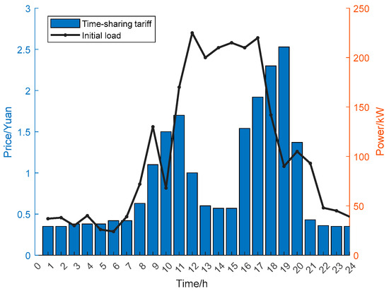
Figure 2.
Time-of-use tariffs and initial load data.
To assess how different factors influence the performance outcomes and associated indicators of the optimization model, four distinct scenarios are designed. These scenarios are created under the same simulation conditions by modifying the factors taken into account and adjusting the optimization strategy or method employed:
- ①
- Scenario 1 addresses the variability in forecasted PV and wind generation, as well as the response of the microgrid users, and based on the user satisfaction with the electricity consumption, it applies the robust optimization model proposed in this paper for the solution;
- ②
- In Scenario 2, the uncertainty in the anticipated output of the renewable power is taken into account, while the response rate of microgrid users is assumed to be 100%. To tackle this issue, the robust optimization model developed in this study is utilized;
- ③
- Scenario 3 applies the microgrid optimal scheduling method proposed in the literature [22] to optimize the problem, and it calculates the user’s comprehensive electricity consumption satisfaction.
5.2. Results and Discussion
The load profile of the microgrid operator after dispatching in Scenario 1 is shown in the following picture, and the operator’s energy storage system and power purchases from the higher grid after optimization are shown in Figure 3.
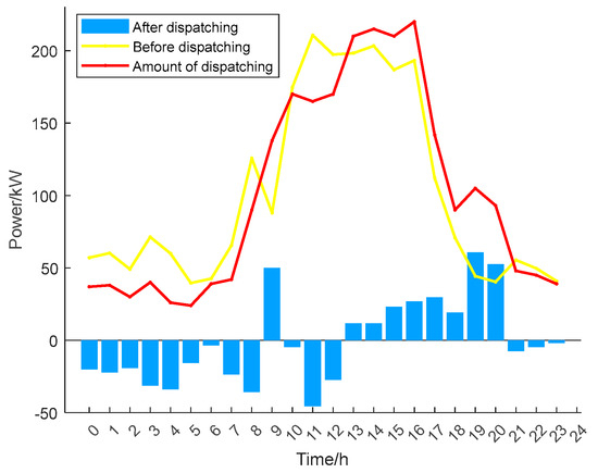
Figure 3.
Load curves before and after scheduling in Scenario 1.
From Figure 3 and Figure 4, it is evident that the load curve becomes smoother following optimization compared to its initial state. In the range of 5~10 h, the output from renewable energy sources sufficiently meets the load demand, though a portion of the generated energy remains unconsumed. This excess energy is first captured by the microgrid operator’s energy storage system. Later, during the peak electricity pricing period of 15~19 h, the stored energy is prioritized for supplying the microgrid loads. This approach not only effectively alleviates the strain on the higher-level grid and prevents the wastage of wind and solar energy but also reduces the microgrid operator’s cluster scheduling expenses, thereby increasing operational profits.
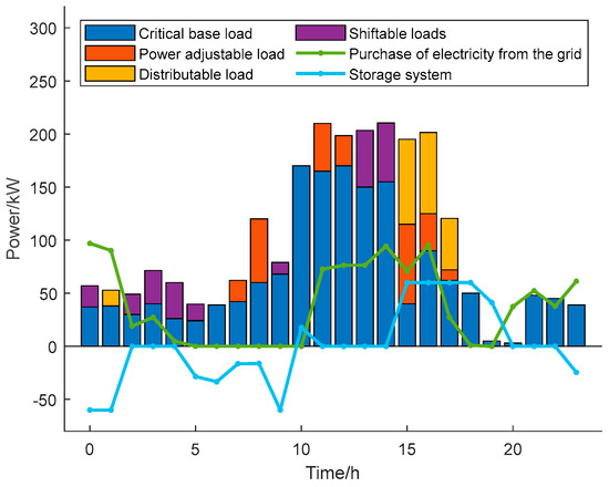
Figure 4.
Scheduling results of each load after optimization.
As shown in Table 2, under the three types of disturbances of electricity price fluctuations, sudden drops in new energy output, and user response deviations, the average satisfaction rate of the method proposed in this paper (98.2%) is significantly higher than that of the stochastic optimization method (87.4%), with an average gap of 10.1%. This verifies the adaptability of the “latent game + robust optimization” framework in an uncertain environment.
Table 2.
Sensitivity analysis.
Table 3 displays the operational outcomes for each scenario. When comparing Scenario 1 to the unoptimized baseline, it becomes clear that implementing cluster scheduling significantly lowers the microgrid operator’s operating costs, thereby greatly enhancing its profits. Additionally, the optimization resolves the issue of unused wind and solar energy, which was previously not fully absorbed, enhancing consumers’ perceived utility toward electricity usage. Furthermore, compared to Scenario 3, the scheduling optimization method introduced in this paper proves to be more effective in reducing the microgrid operator’s costs than other approaches found in the existing literature, particularly by taking into account the users’ satisfaction with their electricity usage.
Table 3.
Operation results of each scenario.
Unlike Scenario 1, Scenario 2 confines uncertainties to renewable energy output, omitting consumer behavioral volatility entirely. As a result, the operator’s operating cost, as shown in Table 1, is reduced. But the electricity consumption habits of some users will be subject to change due to the operator’s cluster scheduling, which improves the economy of electricity consumption of microgrid users to a certain degree, but at the same time, comfort impairment negatively impacts perceived utility, resulting in reduced comprehensive satisfaction among microgrid users. A comparison of the actual loads of Scenario 1 and Scenario 2 is shown in Figure 5.
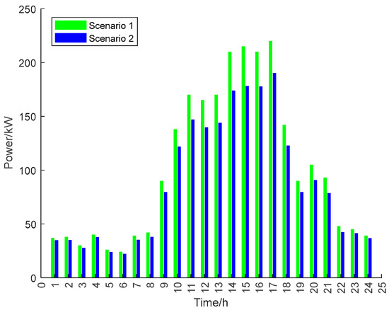
Figure 5.
Scenario 1’s versus Scenario 2’s actual load profiles.
The comparison between Scenario 1 and Scenario 3 verifies that the method in this paper is more practical and instructive in terms of scheduling strategy compared to the method proposed in the literature [22]. From the optimization results, it can be seen that the method proposed in literature [22] will be oriented to time-of-day tariffs, and will be biased towards shifting part of the load from the peak of the tariffs and the nearby hours to the night and the morning, but this will lead to the user’s electricity consumption habits being drastically altered, so that the user’s satisfaction with the electricity consumption will be reduced. As shown in the data in Table 1, although the optimization method in the literature [22] has a lower operating cost than that of the method proposed in this paper, this type of optimization method will lead to a decrease in the customer’s satisfaction with electricity consumption due to scheduling, which in turn affects the customer’s willingness to participate in the scheduling of demand response in the future. A comparison of the results of Scenario 1 and Scenario 3 is shown in Figure 6.
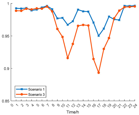
Figure 6.
Scenario 1’s versus Scenario 3’s result profiles.
In summary, this paper validates the effectiveness of the methods proposed in this paper, such as uncertainty and robust optimization, and effectively improves the resilience of operators against the risk of uncertainty by selecting a variety of methods and comparing them with the methods proposed in this paper.
6. Conclusions
This paper proposes a robust optimization strategy for community microgrids, considering multiple uncertainties and focusing on the cluster regulation of various types of load users by community microgrid operators. A model function is established based on the operation cost of community microgrid operators and the comfort level of load users’ electricity consumption. This model maximizes the comprehensive satisfaction of microgrid users’ electricity consumption while the operators are pursuing the operation revenue. The following conclusions can be obtained by analyzing the following arithmetic examples:
- (1)
- Through the cluster control of microgrid operators, the load curve of microgrid users can be improved under the synergy of new energy output, the energy storage system, and the guarantee of higher-level grid, cutting the issue of wind and solar energy curtailment due to incomplete utilization of new energy output, while significantly lowering the operational costs for operators;
- (2)
- Implementing the robust optimization model, after constructing an uncertainty model for the response expectation of the three types of dispatchable loads, minimizes the risk of ad hoc dispatch, enhances the resilience of microgrid system operations, and strengthens the operator’s ability to handle uncertainty during the dispatch process;
- (3)
- The participation of generalized users in operator dispatch and the appropriate adjustment of flexible loads according to time-sharing tariffs can reduce the user’s electricity bill and improve the user’s economy without affecting the user’s comfort, which in turn improves the user’s comprehensive satisfaction.
Under the conditions that the proportion of wind and solar installed capacity is 20–60% and the flexible load-response rate is >70%, this framework can reduce operating costs by 39.1% while maintaining a user satisfaction rate of 98%. It provides a new paradigm for the coordinated optimization of economy and comfort for community microgrids in subtropical climate zones. However, its application scope is still somewhat limited. Future research directions should focus on studying the energy mutual assistance mechanism of community groups, addressing the boundary conditions of cross-community transmission capacity constraints and multi-operator benefit distribution games, so as to adapt to more application scenarios.
Author Contributions
Q.L.: Writing—original draft; C.G.: Writing—review & editing, Resources, Methodology; J.Z.: Formal analysis, Software; Q.Z.: Software, Funding acquisition, Project administration; Y.Y.: Supervision, Writing—review & editing; C.H.: Data curation, Formal analysis. All authors have read and agreed to the published version of the manuscript.
Funding
This research was funded by Power Planning Thematic Research Project of Guangdong Power Grid Corporation, grant number 031000QQ00240017.
Data Availability Statement
The original contributions presented in this study are included in the article. Further inquiries can be directed to the corresponding author.
Conflicts of Interest
Authors Qiang Luo, Chong Gao and Junxiao Zhang were employed by Power Grid Planning Research Center, Guangdong Power Grid Co., Ltd. Authors Qingbin Zeng and Chaohui Huang were employed by the Guangzhou Power Electrical Technology Co., Ltd. The remaining authors declare that the research was conducted in the absence of any commercial or financial relationships that could be construed as a potential conflict of interest.
Appendix A
Based on the definition and nature of latent games, the existence of Nash equilibrium solutions for latent games is proved:
Thus, it can be obtained that
From the above formula, it can be concluded that the definition of the potential game of load in the game model established based on the comprehensive electricity consumption satisfaction of users and the operating costs of community microgrid aggregators possesses all the attributes of potential games. After discretizing the strategy space of this game, if the game model is a finite latent game, then there must be a Nash equilibrium solution for this game.
References
- Ha, T.; Xue, Y.; Lin, K. Optimal Operation of Energy Hub Based Micro-energy Network with Integration of Renewables and Energy Storages. J. Mod. Power Syst. Clean Energy 2022, 10, 100–108. [Google Scholar] [CrossRef]
- Xie, P.; Cai, Z.; Liu, P. Microgrid system energy storage capacity optimization considering multiple time scale uncertainty coupling. IEEE Trans. Smart Grid 2019, 10, 5234–5245. [Google Scholar] [CrossRef]
- Liu, Z.; Yi, Y.; Yang, J. Optimal planning and operation of dispatchable active power resources for islanded multi-microgrids under decentralized collaborative dispatch framework. IET Gener. Transm. Distrib. 2020, 14, 408–422. [Google Scholar] [CrossRef]
- Karimi, H.; Jadid, S. A strategy-based coalition formation model for hybrid wind/PV/FC/MT/DG/battery multi-microgrid systems considering demand response programs. Int. J. Electr. Power Energy Syst. 2022, 136, 107642. [Google Scholar] [CrossRef]
- Parol, M.; Wójtowicz, T.; Ksiezyk, K. Optimum management of power and energy in low voltage microgrids using evolutionary algorithms and energy storage. Int. J. Electr. Power Energy Syst. 2020, 119, 105886. [Google Scholar] [CrossRef]
- Singh, B.; Bishnoi, S.; Sharma, M. An application of nature inspried algorithm based dual-stage frequency control strategy for multi micro-grid system. Ain Shams Eng. J. 2023, 14, 102125. [Google Scholar] [CrossRef]
- Chen, Q.; Wang, W.; Wang, H. Coordinated optimization of active distribution network with multiple microgrids considering demand response and mixed game. Autom. Electr. Power Syst. 2023, 47, 99–109. [Google Scholar]
- Ashwin, S.; Valliappan, M.; Victor, D. A Secure and Adaptive Hierarchical Multi-Timescale Framework for Resilient Load Restoration Using a Community Microgrid. IEEE Trans. Sustain. Energy 2023, 14, 1057–1075. [Google Scholar] [CrossRef]
- Xiong, X.; Yang, H.; Cai, Y. Robust optimal dispatch method of microgrid considering user endowment effect and environmental awareness un-certainty. Proc. CSEE 2023, 43, 8260–8270. [Google Scholar]
- Shahnewaz, S.; Kofi, A.; Ken, B. A Data-Driven Framework for Quantifying Demand Response Participation Benefit of Industrial Consumers. IEEE Trans. Ind. Appl. 2024, 60, 2577–2587. [Google Scholar]
- Cui, D.; Lu, C.; Tang, H.; Gong, S.; Yang, Z.; Liu, W. Dynamic Pricing and Energy Management of Electric Heating Integrated Energy System Based on Master-Slave Game Theory. In Proceedings of the 2023 3rd International Conference on New Energy and Power Engineering (ICNEPE), Huzhou, China, 24–26 November 2023; pp. 40–44. [Google Scholar]
- Zhang, T.; Li, Y.; Yan, R.; Abu-Siada, A.; Guo, Y.; Liu, J.; Huo, R. A Master-Slave Game Optimization Model for Electric Power Companies Considering Virtual Power Plant. IEEE Access 2022, 10, 21812–21820. [Google Scholar] [CrossRef]
- Liu, D.; Zeng, Q.; Zhang, Y. Spatio-temporal adaptation assessment of new distribution network key technologies based on 3D space. J. Shanghai Jiaotong Univ. 2024, 58, 1489–1499. [Google Scholar]
- Abdullah, U.; Deepak, K.; Tirthadip, G. Decentralized Community Energy Management: Enhancing Demand Response Through Smart Contracts in a Blockchain Network. IEEE Access 2024, 12, 80781–80798. [Google Scholar] [CrossRef]
- Liu, D.; Zeng, Q.; Zhang, Y. Optimal energy scheduling strategy of building groups considering multiple uncertainties and potential game. Electr. Power Autom. Equip. 2024, 44, 136–144. [Google Scholar]
- Sahar, S.; Behnam, M.; Mehdi, A.; Miadreza, S. Optimal Sizing and Siting of Electric Vehicle Charging Stations in Distribution Networks With Robust Optimizing Model. IEEE Trans. Intell. Transp. Syst. 2024, 25, 4314–4325. [Google Scholar]
- Liu, Z.; Liu, S.; Li, Q. Optimal Day-ahead Scheduling of Islanded Microgrid Considering Risk-based Reserve Decision. J. Mod. Power Syst. Clean Energy 2021, 9, 1149–1160. [Google Scholar] [CrossRef]
- Liu, D.; Xu, Z.; Zhong, K. Optimal Scheduling of Flexible Loads for New Building Clusters Considering Potential Games. In Proceedings of the 2023 8th International Conference on Power and Renewable Energy (ICPRE), Shanghai, China, 22–25 September 2023; pp. 571–577. [Google Scholar]
- Gao, J.; Yang, Y.; Gao, F. Two-Stage Robust Economic Dispatch of Regional Integrated Energy System Considering Source-Load Uncertainty Based on Carbon Neutral Vision. Energies 2022, 15, 1504–1596. [Google Scholar] [CrossRef]
- Danial, Y.; Mohammad, N.; Donya, Y.; Jürgen, B.; Trung, T.; Amir, H. Robust Optimization Over Time: A Critical Review. IEEE Trans. Evol. Comput. 2024, 28, 1265–1285. [Google Scholar]
- Li, X.; Wang, J.; Lu, Z. Pricing strategy of energy service provider based on non-cooperative game and revenue sharing contract. Electr. Power Autom. Equip. 2022, 42, 1–8. [Google Scholar]
- Hou, Y.; Zeng, J.; Luo, Y. Research on collaborative and optimization methods of active energy management in community microgrid. Power Syst. Technol. 2023, 47, 1548–1557. [Google Scholar]
Disclaimer/Publisher’s Note: The statements, opinions and data contained in all publications are solely those of the individual author(s) and contributor(s) and not of MDPI and/or the editor(s). MDPI and/or the editor(s) disclaim responsibility for any injury to people or property resulting from any ideas, methods, instructions or products referred to in the content. |
© 2025 by the authors. Licensee MDPI, Basel, Switzerland. This article is an open access article distributed under the terms and conditions of the Creative Commons Attribution (CC BY) license (https://creativecommons.org/licenses/by/4.0/).