Abstract
Atmospheric aerosols significantly impact solar photovoltaic (PV) energy generation through their effects on surface solar radiation. This study quantifies the impact of PM2.5 pollution on PV power output using observational data from 10 stations across Hebei Province, China (2018–2019). Our analysis reveals that elevated PM2.5 concentrations substantially attenuate solar irradiance, resulting in PV power losses reaching up to a 48.2% reduction in PV power output during severe pollution episodes. To capture these complex aerosol–radiation–PV interactions, we developed and compared the following six machine learning models: Support Vector Regression, Random Forest, Decision Tree, K-Nearest Neighbors, AdaBoost, and Backpropagation Neural Network. The inclusion of PM2.5 as a predictor variable systematically enhanced model performance across all algorithms. To further optimize prediction accuracy, we implemented a stacking ensemble framework that integrates multiple base learners through meta-learning. The optimal stacking configuration achieved superior performance (MAE = 0.479 MW, indicating an average prediction error of 479 kilowatts; R2 = 0.967, reflecting that 96.7% of the variance in power output is explained by the model), demonstrating robust predictive capability under diverse atmospheric conditions. These findings underscore the importance of aerosol–radiation interactions in PV forecasting and provide crucial insights for grid management in pollution-affected regions.
1. Introduction
Solar photovoltaic (PV) technology is one of the most critical renewable energy solutions available today. Since the Industrial Revolution, the reliance on fossil fuels has led to severe environmental pollution and resource depletion, threatening our living environment and sparking serious considerations of sustainable development [1]. In this context, PV technology, which harnesses the widely available and abundant solar energy [2], offers a promising avenue to mitigate the global energy crisis and substantially improve the current ecological environment [3]. Therefore, in-depth research into the development and application of solar photovoltaic technology across various sectors holds significant practical and strategic value.
The basic principle of solar photovoltaic power generation involves converting sunlight into electricity using solar panels. When sunlight passes through the atmosphere and is absorbed by these panels, the solar cells within generate electricity [4]. Consequently, the power output of solar photovoltaic stations is influenced by solar radiation, which consists of global horizontal irradiance (GHI) and diffuse horizontal irradiance (DHI) [5]. GHI represents the solar energy that passes through Earth’s atmosphere and reaches a horizontal surface, serving as the dominant factor in photovoltaic power generation. However, GHI is influenced by various meteorological factors [6], making it challenging to accurately predict the power output of photovoltaic stations. Unlike GHI, DHI is composed of scattered, indirect radiation and contributes relatively less to photovoltaic power generation. Nevertheless, DHI remains an important component and should not be overlooked. DHI is primarily affected by factors such as cloud cover and atmospheric aerosols [7], with PM2.5 being particularly significant. PM2.5 refers to fine particulate matter with a diameter of less than 2.5 microns, which can scatter and absorb solar radiation, thereby impacting DHI [8]. PM2.5 concentrations are inversely correlated with DHI levels and consequently affect power generation efficiency.
The physical mechanisms through which PM2.5 affects PV performance follow well-established atmospheric optics principles. According to Mie scattering theory, particles with diameters comparable to solar wavelengths (0.1–2.5 μm) significantly scatter and attenuate solar radiation [9]. The attenuation process can be described by the Beer–Lambert law, as follows:
where I(λ) denotes the irradiance reaching the PV module, IO(λ) is the extraterrestrial irradiance, τ(λ) is the aerosol optical depth induced by PM2.5, and m is the air mass. The aerosol optical depth is further determined by the following:
where σext is the mass extinction coefficient, and N(z) is the vertical concentration of PM2.5. The expected mechanisms include [10,11,12] the following:
Scattering effect (dominant): particulate matter deflects solar radiation, reducing direct irradiance.
Absorption effect: light-absorbing aerosols such as black carbon absorb solar energy.
Multiple scattering: under heavy pollution, radiation attenuation is further amplified.
Research has increasingly underscored the significance of aerosols, particularly PM2.5, on solar PV performance across diverse international contexts with similar industrial air quality challenges. Studies from India demonstrate substantial regional impacts, with Ghosh et al. (2022) documenting that atmospheric pollution caused India to lose 29% of its solar energy potential between 2001–2018, equivalent to an annual loss of USD 835 million [13]. Recent projections by Ghosh et al. (2024) indicate that India’s PV efficiency could decline nationally by 2.3–3.3% by mid-century, with potential power losses as high as 840 GWh annually due to combined climate change and air pollution effects [14]. For instance, Song et al. (2022) demonstrated that PM2.5, as a key component of aerosols, can reduce global horizontal irradiance by over 5% during months when concentrations exceed 33.5 μg/m3, resulting in average energy output losses of 7.00% for crystalline silicon and 9.73% for thin-film PV systems [15]. These studies highlight the considerable environmental risk that PM2.5 poses to solar energy production. Similarly, Sun et al. (2018) reported that aerosol deposition on PV panel surfaces significantly reduces transmittance. Their findings indicated that under short-term aerosol exposure, transmittance at 18.7 μg/cm2 averaged 96.4%. However, as the exposure duration increased, the reduction in transmittance became more severe, with decreases ranging from 42.1% to 118.1% compared to clean panels [16]. This aligns with research showing that high concentrations of PM2.5 can lead to substantial declines in solar energy production, particularly during peak pollution episodes. Recent studies further validate these theoretical expectations. For example, Kim et al. (2024) report that even a 10 μg/m3 increase in PM2.5 concentration in South Korea significantly reduces solar power generation, especially under direct irradiance conditions [17]. This aligns with the predicted nonlinear transition from moderate to strong attenuation once certain pollution thresholds are surpassed. The cumulative evidence highlights the need for ongoing investigation into the effects of PM2.5, particularly in regions with significant air pollution, where PV systems may experience frequent and substantial efficiency losses.
Hebei Province serves as a representative region for studying PM2.5 pollution impacts on PV systems, combining significant solar energy potential with severe air pollution challenges. The province possesses considerable PV development opportunities due to its abundant solar resources and extensive land availability [18,19,20]. However, its industrial structure and diverse pollution sources contribute to frequent PM2.5 pollution events [21,22,23,24], significantly compromising PV system efficiency. These environmental challenges create a unique context for investigating the PM2.5-PV relationship. Quantifying this relationship is essential for optimizing PV system performance and informing the planning, operation, and management strategies of photovoltaic facilities in high-pollution regions.
Quantifying PM2.5’s impact on PV power generation has been approached through various methodologies. Traditional physical models simulate the interactions between solar radiation and atmospheric conditions to predict power output [25,26,27]. While these models incorporate fundamental parameters, such as solar irradiance and meteorological data, they often show limitations in accuracy when system configurations or environmental conditions fluctuate [28]. Machine learning models have emerged as a more robust alternative, offering enhanced predictive capabilities through data-driven approaches. These models learn complex relationships from historical data, capturing both linear and nonlinear interactions among factors affecting PV performance [29]. Different machine learning algorithms exhibit distinct advantages, as follows: Artificial neural networks (ANNs) excel in modeling nonlinear relationships and complex patterns [30], while support vector machines (SVMs) demonstrate particular strength with limited samples and high-dimensional datasets [31]. Decision trees and random forests offer additional benefits through their interpretable structure and robust handling of missing data. Thus, the selection of an appropriate machine learning model depends critically on specific application requirements, data characteristics, and computational resources. This choice significantly influences the accuracy and reliability of PV power predictions under varying environmental conditions. From a theoretical perspective, different machine learning models exhibit complementary strengths in capturing the complex effects of PM2.5. Random Forests are well-suited for identifying variable interactions and threshold behaviors [32]. Support Vector Regression leverages kernel functions to model nonlinear attenuation dynamics. Neural networks, particularly multilayer perceptrons, can learn spatiotemporal dependencies in PM2.5 impacts under varying meteorological regimes [33,34]. Although machine learning models are widely applied in PV power generation prediction [35], existing research has primarily focused on regions such as the Yangtze River Delta [36,37,38,39,40,41], with limited studies examining Hebei Province. To address this research gap, this study pursues the following three primary objectives: (1) to analyze the temporal and spatial characteristics of PV output across Hebei Province using operational data from 10 photovoltaic stations during the period of July 2018 to June 2019; (2) to quantify the impact of PM2.5 on photovoltaic power generation utilizing the Himawari-8 Hourly 5 km Ground-Level PM2.5 Dataset; and (3) to develop an enhanced prediction framework for PV power output through the implementation of multiple machine learning models, including Support Vector Regression (SVR), Random Forest (RF), Decision Tree (DT), Adaptive Boosting (AdaBoost), K-Nearest Neighbor (KNN), and Backpropagation Neural Network (BP), integrated within a stacking framework to optimize prediction performance.
2. Materials and Methods
2.1. Study Sites and Data
This study focuses on ten PV sites in Hebei Province, China (Figure 1). As a key region for PV power generation in northern China, Hebei Province spans 197,900 square kilometers. In 2020, its PV power generation potential was 40.1 billion kWh, representing 1% of the national total [19]. The southern part of Hebei Province presents substantial potential for PV development, driven by its diverse resources. Rooftops offer the highest theoretical generation capacity, estimated at 64,032 GWh. Additionally, water bodies, roadways, and unused land collectively contribute a further 131,306 GWh in potential PV developments [18], highlighting the region’s significant opportunities for PV expansion. Given the high electricity demand in urban areas, especially those with “low generation, high consumption”, prioritizing PV development in these locations is crucial. Thus, focusing on these high-potential areas within southern Hebei could greatly enhance the region’s contribution to national PV power generation.
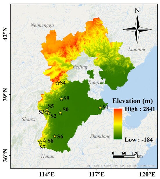
Figure 1.
Spatial distribution of 10 PV stations across Hebei Province.
The photovoltaic dataset used in this study can be freely downloaded from GitHub (https://github.com/yaotc/PVODataset) (accessed on 1 April 2024) [5]. The PVOD dataset comprises 271,968 records from 10 PV sites with 15-minute intervals, covering the period from 1 July 2018 to 13 June 2019. It integrates photovoltaic power outputs, local measurement data (LMD), and numerical weather prediction (NWP) data. The meteorological parameters recorded include global and diffuse irradiance, temperature, pressure, wind direction, and wind speed (see Table 1). The elevation data used in Figure 1 were sourced from the Geospatial Data Cloud (https://www.gscloud.cn/) and derived from the ASTER GDEM with a 30 m spatial resolution. Elevation values across Hebei Province range from −184 m to 2841 m, allowing for an intuitive depiction of the geographic setting of each photovoltaic station and facilitating the analysis of topography-related environmental influences on PV performance.

Table 1.
Key meteorological variables and model performance metrics for PV power output prediction.
The ChinaHighPM2.5 dataset used in this study is freely available from https://zenodo.org/records/6398971 (accessed on 12 May 2024) [42,43]. This dataset offers a comprehensive and high-resolution record of ground-level PM2.5 concentrations across China from 2000 to 2021. As part of the ChinaHighAirPollutants (CHAP) series, it is generated using a combination of ground-based measurements, satellite remote sensing, atmospheric reanalysis, and model simulations, with artificial intelligence employed to account for the spatiotemporal variability of air pollution. The dataset offers complete spatial coverage at a 1 km resolution and is available in daily, monthly, and yearly formats. It is highly accurate, with a cross-validation coefficient of determination (CV-R2) of 0.92, a root mean square error (RMSE) of 10.76 µg/m3, and a mean absolute error (MAE) of 6.32 µg/m3 on a daily basis.
To ensure the reliability and authenticity of our analysis, we adopted a conservative approach to missing data handling. Rather than employing imputation techniques, we chose to work exclusively with directly observed, quality-controlled data from the PVOD dataset. This methodological decision prioritizes data integrity over completeness, as our primary objective was to develop and validate machine learning models using authentic observational records. Missing data points in our analysis (as presented in figures in Section 3.1.1) represent periods where direct measurements were unavailable, and we maintained these gaps to preserve the genuine temporal patterns in the dataset. This approach aligns with best practices in environmental modeling where the authenticity of input data is crucial for developing reliable predictive frameworks for real-world applications.
2.2. Methods
2.2.1. Software Implementation and PVOD Dataset Processing Framework
This study was implemented using Python 3.10 in PyCharm 2021.3 Professional Edition with the following key libraries: scikit-learn 1.5.1 for machine learning algorithms, pandas 2.2.1 for data manipulation, numpy 1.26.4 for numerical computations, matplotlib 3.8.3 for visualization, and scipy 1.13.0 for statistical analysis.
The PVOD dataset from GitHub contained metadata.csv and station00.csv to station09.csv files representing 10 photovoltaic stations. The software systematically loaded each station’s data using pandas.read_csv(), extracted geographic coordinates from metadata through index-based selection, and integrated PM2.5 concentrations via spatiotemporal matching based on coordinates and time alignment. This process generated processed datasets named processed_with_pollution_S{station_id}_corrected.csv for each station.
Six machine learning models were implemented using scikit-learn’s default solver configurations with hyperparameters optimized through five-fold cross-validation grid search. SVR utilized RBF kernel with libsvm solver for nonlinear regression, RandomForestRegressor employed bootstrap aggregating for ensemble learning, DecisionTreeRegressor implemented CART algorithm for hierarchical partitioning, AdaBoostRegressor applied adaptive boosting for iterative improvement, KNeighborsRegressor used distance-based local approximation, and MLPRegressor employed Adam optimizer for neural network training with backpropagation.
The stacking ensemble framework was implemented in stacking_ensemble_training.py using StackingRegressor, systematically combining five base learners with one meta-learner across six configurations through itertools.combinations(). As shown in Figure 2, the stacking training process demonstrates the PyCharm development environment with organized project structure, core implementation code, and real-time execution of comprehensive evaluation metrics (MSE, RMSE, MAE, MAPE, R2) for multiple stacking combinations.
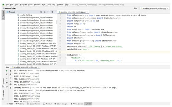
Figure 2.
Screenshot of stacking ensemble training process in PyCharm development environment, showing the project structure, model implementation code, and real-time evaluation metrics for multiple stacking combinations.
The software implementation provides the following three key technical contributions: (1) automated PVOD dataset integration pipeline that processes original station files and incorporates PM2.5 data through coordinate-based spatiotemporal matching, (2) comprehensive stacking ensemble framework that systematically evaluates all possible six-model combinations with optimized hyperparameters, and (3) reproducible analysis workflow with real-time performance monitoring and automated result logging across multiple photovoltaic stations.
2.2.2. Criteria for Selecting PM2.5 Pollution Levels and Background Days
To examine the effects of varying pollution levels on PV power output, this study categorizes pollution conditions during the observation period into three levels according to the environmental air quality criteria issued by the Ministry of Environmental Protection of China, as follows: clean-air days (with a daily average PM2.5 concentration of 0–75 µg/m3), moderately polluted days (with a daily average PM2.5 concentration of 75–150 µg/m3), and heavily polluted days (with a daily average PM2.5 concentration exceeding 150 µg/m3) [44]. Additionally, to explore the seasonal patterns of pollution, the data are further divided into spring (March to May), summer (June to August), autumn (September to November), and winter (December to February). Findings indicate that pollution events tend to occur more frequently in the autumn and winter seasons, providing valuable insights into the seasonal variations of PV power output under different air quality conditions.
2.2.3. Machine Learning Models
To enhance the predictive accuracy of PV power forecasting under varying air pollution conditions, this study employs the following six widely used machine learning algorithms: SVR, RF, DT, AdaBoost, KNN, and BP [45,46,47]. These models represent a diverse range of algorithmic paradigms—including kernel-based learning, ensemble methods, decision rule systems, instance-based approaches, and neural network structures—allowing for a comprehensive evaluation across heterogeneous data characteristics and pollution regimes. Each model is built upon specific theoretical assumptions that influence its suitability for PV forecasting under environmental variability, particularly in the presence of PM2.5 pollution.
SVR assumes that the underlying relationship between predictors and the target variable can be approximated by a function that maximizes the margin of tolerance (ε) while minimizing model complexity, in accordance with structural risk minimization principles. Through kernel functions such as the radial basis function (RBF), SVR effectively captures nonlinear interactions among meteorological inputs and pollution indicators. Its strong generalization ability and robustness to overfitting make it particularly effective in noisy, small-sample, or pollution-sensitive scenarios. RF is grounded in the assumption that aggregating multiple weak, decorrelated decision trees—each trained on different bootstrap samples and random subsets of features—produces a robust predictor with enhanced accuracy and generalization. Its ensemble structure mitigates variance and handles high-dimensional, noisy data effectively. These properties make RF especially suitable for modeling the complex and nonlinear interactions between PV output and environmental variables such as irradiance, temperature, and PM2.5. DT relies on the assumption that hierarchical partitioning of the data based on information gain can reveal interpretable decision rules that govern the output. This makes DT valuable for identifying dominant features affecting PV output, such as PM2.5 levels. However, its sensitivity to training data structure and limited generalization in volatile conditions may reduce its robustness under fluctuating pollution scenarios. AdaBoost assumes that predictive performance can be iteratively improved by focusing successive weak learners on misclassified instances. This adaptive mechanism enables the model to detect sharp variations in PV output driven by transient environmental disturbances, such as PM2.5 spikes. Nevertheless, its tendency to overfit noisy inputs may hinder its stability in highly dynamic conditions. KNN operates under the assumption that data points in close proximity within the feature space will yield similar outputs. While its simplicity and non-parametric nature make it well-suited for capturing localized variations in PV output under stable conditions, KNN is highly sensitive to data density and may struggle when pollution patterns are sparse or rapidly changing. BP is based on the assumption that complex, nonlinear mappings between inputs and outputs can be learned through multi-layer forward propagation and gradient-based error backpropagation. It excels at capturing intricate variable interactions—such as those involving irradiance, temperature, and PM2.5—but requires careful hyperparameter tuning and sufficient data to avoid overfitting, particularly under noisy or heterogeneous environmental conditions.
By aligning model selection with their underlying assumptions and methodological strengths, this study provides a robust basis for evaluating the predictive impact of PM2.5 on PV output. This alignment ensures that each model is applied in a contextually appropriate manner, enhances interpretability, and improves the reliability of conclusions drawn under variable atmospheric conditions.
2.2.4. Experiment Design
To rigorously evaluate the predictive value of PM2.5 concentration in PV power forecasting, a structured experiment was designed comprising the following four key components: (1) model selection, (2) input variable configuration, (3) model training and hyperparameter optimization, and (4) stacking ensemble framework. The experimental design aimed to assess both the standalone performance of various machine learning models and the benefit of incorporating PM2.5 data under controlled, comparative conditions.
- (1)
- Model Selection
To support a robust comparative analysis of forecasting strategies under varying pollution conditions, the following six machine learning models were selected: SVR, RF, DT, AdaBoost, KNN, and BP. These models collectively represent a broad spectrum of algorithmic paradigms, encompassing kernel-based methods, ensemble techniques, rule-based decision processes, local similarity approaches, and deep learning architectures. The selection was guided by the need to capture diverse data behaviors, including nonlinear patterns, noise sensitivity, spatial–temporal variability, and overfitting risks. Detailed descriptions of each model’s theoretical assumptions, computational characteristics, and applicability to PV power forecasting under PM2.5 influence are provided in Section 2.2.2. This model set forms a balanced foundation for evaluating not only standalone performance but also responsiveness to pollution-aware input configurations.
- (2)
- Input variable configuration
To rigorously assess the predictive contribution of PM2.5 in PV power forecasting, two input configurations were established. The PM2.5-inclusive setting comprised all seven predictors—WD, WS, DHI, GHI, T, P, and PM2.5. In contrast, the PM2.5-free setting excluded only the PM2.5 variable, while retaining the remaining six features unchanged. This controlled input design enables a direct, feature-isolated comparison of model performance with and without air pollution information. By maintaining identical input conditions across both configurations—except for the presence of PM2.5—any performance difference can be attributed specifically to the added value of pollution data. To ensure consistency, both configurations were applied uniformly to all sites and models throughout the experimental process.
- (3)
- Model Training and Hyperparameter Optimization
Model training and optimization were performed using a consistent procedure across all PV sites. Each site’s dataset was chronologically partitioned into a training set (80%) and a testing set (20%) to preserve the temporal structure and prevent information leakage. Input features were preprocessed according to the scaling requirements of each model. Specifically, SVR and BP were standardized using z-score normalization to ensure numerical stability during kernel-based mapping and gradient-based learning. KNN, which relies on distance computations, was normalized using min–max scaling to maintain the relative geometry of the feature space. In contrast, tree-based and ensemble models—namely, RF, DT, and AdaBoost—were trained on unscaled inputs, as their split-based architectures are inherently robust to feature magnitude.
To ensure a robust and fair model comparison, hyperparameter tuning was conducted using a comprehensive grid search combined with five-fold cross-validation. This procedure followed the preprocessing strategy described above, with scaling operations integrated consistently into the training pipeline. To enhance reproducibility, the cross-validation folds were randomly shuffled using a fixed random seed. Model performance was evaluated based on the coefficient of determination (R2), which served as the primary criterion for selecting the optimal parameter configuration. The full set of hyperparameter configurations explored during model optimization is provided in the Table S1, which outlines the complete grid search ranges for each model. For SVR, tuning involved the regularization parameter and the ε-insensitive loss margin, jointly controlling model complexity and tolerance to prediction errors. For RF and DT, the optimization focused on structural parameters, including maximum tree depth, minimum samples required for node splitting, and minimum samples per leaf. AdaBoost was optimized by varying the number of estimators and learning rate to adjust ensemble capacity and convergence behavior. For KNN, the number of neighbors and the choice of distance weighting method were adjusted to improve local approximation performance. For BP, tuning encompassed both architectural and training-related parameters, including network configurations with one or two hidden layers of varying sizes and the learning rate scheduling strategy. The optimal hyperparameter combinations and corresponding training results obtained from five-fold cross-validation at each site are archived in Tables S2–S11. These files document the best-performing parameter sets for each model and site, along with the associated R2, RMSE, MAE, and MSE scores on the training set. This collection provides a transparent basis for model comparison and supports reproducibility across both PM2.5-inclusive and PM2.5-free scenarios.
Once the optimal hyperparameter configurations were identified through cross-validation, each model was retrained on the full training set using its respective best parameters and subsequently applied to predict PV power output on the hold-out testing set. This evaluation strategy ensured that model performance was assessed under realistic, unseen conditions, thereby providing a more generalizable estimate of forecast accuracy. To systematically investigate the influence of air pollution, the following two input settings were adopted in parallel: one that included PM2.5 concentration as a predictor (PM2.5-inclusive), and one that excluded it (PM2.5-free). This dual-scenario design enabled direct comparison of model behavior under varying environmental complexity. The relative differences in prediction accuracy across these conditions served as the basis for assessing the sensitivity of different algorithms to PM2.5 information and its role in improving forecasting performance.
- (4)
- Stacking Ensemble Framework
To further enhance the accuracy and robustness of PV power forecasting, a stacking ensemble framework was employed. Stacking integrates the predictions of multiple base learners through a meta-model, leveraging the diversity of individual algorithms to capture nonlinear dependencies and residual errors that single models may overlook. Figure 3 illustrates the fundamental principles of stacking, showcasing how different algorithms can be synergistically combined to capitalize on their respective strengths and achieve improved overall performance. Building upon this framework, we implemented a two-level stacking model tailored for PV power prediction under varying air quality conditions. The architecture consisted of a hierarchical structure with two layers. The first layer comprised five base learners selected from a pool of six models—SVR, RF, DT, AdaBoost, KNN, and BP. The second layer functioned as a meta-learning module, using the remaining model—that is, the one not included in the first layer—as the meta-learner to integrate the predictions of the base learners. This design resulted in six distinct stacking configurations (Comb 1 through Comb 6), each representing a unique permutation of five base learners and one meta-learner. Such a construction enabled the systematic evaluation of the individual contribution of each model both as a base learner and as a meta-learner within the ensemble framework.
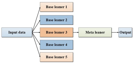
Figure 3.
Schematic representation of the stacking ensemble learning framework.
Each stacking configuration was trained using the same experimental setup as the individual models to ensure methodological consistency. Specifically, each site’s dataset was split chronologically into a training set (80%) and a testing set (20%), identical to the data partitioning used for single-model training and evaluation. For each configuration, the five selected base learners were trained using their respective optimal hyperparameters as determined in the cross-validation procedure described in Section 2.2.3 (3). The remaining model, designated as the meta-learner, was likewise trained on the outputs of the base learners using its previously optimized hyperparameter settings. This consistent reuse of validated parameter configurations ensured that performance differences could be attributed solely to ensemble design rather than to disparities in model tuning. To evaluate the efficacy of ensemble learning relative to individual modeling approaches, all stacking configurations (Comb 1 through Comb 6) were systematically compared against the six single-model baselines described in Section 2.2.3. The comparison was performed across ten PV sites using identical training–testing splits, consistent input settings, and the same set of evaluation metrics (R2 and MAE). Each stacking configuration was trained and tested under both PM2.5-inclusive and PM2.5-free scenarios, thereby enabling a controlled investigation of the role of pollution-related features in forecasting performance. This comparative design served two key analytical purposes. First, it allowed for assessing whether stacking ensembles deliver a measurable performance advantage over their individual components across diverse spatial and environmental conditions. Second, it provided a means to quantify the added predictive value of PM2.5 concentration as an input variable, both within single-model frameworks and ensemble structures. By examining variations in prediction error and correlation across different configurations and input types, this strategy facilitated a comprehensive analysis of algorithmic complementarity and environmental feature relevance in the context of PV power forecasting.
2.2.5. Evaluation Metrics
In this study, the evaluation framework for assessing the predictive performance of models forecasting PV power generation under varying PM2.5 pollution conditions includes several critical statistical metrics, as follows: the coefficient of determination (R2), root mean squared error (RMSE), mean absolute error (MAE), mean squared error (MSE), standard deviation (STD), and mean absolute percentage error (MAPE). These metrics are defined as follows:
In these metrics, represents the number of samples, denotes the actual observed value for the sample, signifies the predicted value for the sample, and is the mean of all observed values. R2 indicates the proportion of variance in the dependent variable that is explained by the independent variables, with values ranging from 0 to 1. A value close to 1 suggests a high quality of model fit, while a value near 0 indicates a poor fit. RMSE is the square root of the average squared differences between observed and predicted values, reflecting the standard deviation of prediction errors and quantifying the discrepancy between model predictions and actual observations; a smaller RMSE indicates fewer prediction errors. MAE calculates the average of the absolute differences between observed and predicted values, providing a direct measure of the average magnitude of prediction errors. Unlike RMSE, MAE does not disproportionately penalize larger errors, allowing for a more balanced assessment of error magnitudes. MSE is the average of the squared differences between observed and predicted values, serving as a measure of the model’s overall accuracy. MAPE measures the model’s accuracy as a percentage by averaging the absolute percentage differences between observed and predicted values. STD captures the variability or dispersion of the predicted values around their mean. In the context of PV power forecasting and Taylor diagram analysis, STD is used to evaluate how well a model replicates the fluctuation patterns of the observed data. Collectively, these metrics offer a comprehensive evaluation of the model’s predictive performance.
3. Results
3.1. Spatiotemporal Dynamics of PV Power Output
3.1.1. Temporal Variation Characteristics
The ten PV sites in Hebei Province exhibited significant diurnal and seasonal variation patterns during July 2018 to June 2019. As illustrated in Figure 4, daily PV power generation follows a clear diurnal pattern; power output increases steadily after sunrise, peaks around midday, and gradually declines toward sunset. This cycle demonstrates the direct relationship between PV output and solar irradiance intensity.
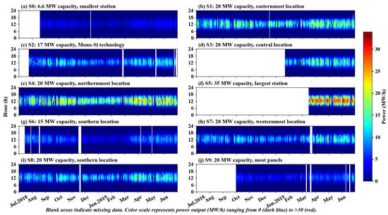
Figure 4.
Spatiotemporal distribution of photovoltaic power generation at 10 stations in Hebei Province (July 2018–June 2019).
Seasonal variations in PV power generation reveal critical dynamics, particularly at site S1. During spring and summer, the average PV output reached 16.85 MW/h, representing a 31.8% increase compared to the autumn and winter. This increase primarily results from longer daylight hours and higher solar angles [48], which enhance solar radiation intensity and power generation. Conversely, autumn and winter showed reduced PV output, averaging 12.78 MW/h. This reduction stems from lower solar angles, shorter daylight periods, and the adverse effects of air pollutants, particularly PM2.5. Elevated PM2.5 levels absorb and scatter sunlight, reducing PV module efficiency [49], especially in winter. Data from site S4 between July 2018 and June 2019 further confirm these patterns. July and August showed average outputs of 15.80 MW/h and 17.11 MW/h, respectively, with peak output reaching 21.07 MW/h in October. However, winter experienced a significant decline to an average of 14.33 MW/h. This decrease primarily reflects reduced solar exposure during winter, compounded by high PM2.5 concentrations.
Generally, these findings demonstrate that optimizing PV systems requires considering both diurnal solar variations and seasonal environmental changes. Future predictive models should incorporate both climatic and pollution conditions to improve PV system efficiency.
3.1.2. Spatial Variation Characteristics
The spatial distribution of PV output across the ten stations in Hebei Province reveals significant differences influenced by geographic location and local environmental conditions. Figure 4 illustrates the temporal power generation patterns across these stations, while Table 2 provides a comparative analysis of the monthly average power outputs, highlighting the spatial variability in PV performance. Geographic location plays a crucial role in determining PV output. Stations in southern Hebei, such as site S5, exhibit notably higher average monthly outputs. Site S5 achieves an average monthly power output of 27.76 MWh, benefiting from longer sunshine hours and higher solar radiation. This enhanced solar exposure in the southern region leads to consistently higher PV generation compared to stations in less favorable conditions. Conversely, stations in northern and eastern Hebei, such as S9, show considerably lower power outputs, averaging only 5.69 MWh monthly. The reduced output at these stations results from multiple factors, including limited solar exposure due to geographic and topographic features and increased atmospheric pollution [50,51,52]. These locations often feature complex terrain, such as hills and mountains, which obstruct solar radiation and diminish PV efficiency [53].
Table 2.
Monthly average PV output for ten stations in Hebei.
In addition to geographic location, local environmental conditions, particularly air quality, significantly impact PV performance. Stations in areas with higher PM2.5 levels experience lower power outputs. PM2.5 and other aerosols attenuate solar radiation reaching PV modules, reducing energy generation. This effect becomes particularly evident in regions with frequent high pollution episodes, as shown by lower outputs during months with elevated PM2.5 concentrations. Table 2 presents the monthly average power output for each PV station, demonstrating spatial performance heterogeneity. When combined with Figure 1, which shows the spatial distribution of the ten PV stations across Hebei Province, these variations become more apparent. Analysis of Table 3 and Figure 3 reveals that southern stations consistently outperform those in northern and eastern areas, highlighting the influence of geographic and environmental factors on PV system efficiency. These spatial variations emphasize the need for location-specific optimization strategies. Understanding these spatial differences is essential for developing effective forecasting models and improving PV system performance across diverse locations.
Table 3.
Average performance metrics of machine learning models for PV power forecasting: comparative analysis under PM2.5 conditions.
3.2. The Response of PV Power Generation Dynamics to PM2.5 Pollution
Temperature, wind speed, wind direction, and atmospheric pressure are key factors affecting PV output—temperature directly impacts cell efficiency, wind conditions regulate module cooling, while atmospheric pressure serves as an indicator of pollution variations. PV power output exhibits significant seasonal variability (Figure 4), as do PM2.5 levels and certain meteorological factors such as temperature and wind speed [54]. Notably, autumn and winter seasons experience concentrated pollution, compounded by low temperatures and inversion effects, which may significantly impact PV performance [55]. On clean days, wind speeds are generally higher, with a mean value of approximately 1.23 m/s. In contrast, on moderate pollution days, wind speed decreases to a mean of around 0.93 m/s, and on heavy pollution days, wind speeds are at their lowest, averaging about 0.75 m/s. Wind direction, however, remains consistent across all pollution levels, showing no significant correlation with PM2.5 concentrations, and fluctuates between 0° and 360° (Figure 5).
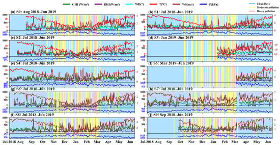
Figure 5.
Temporal variations of meteorological variables under different PM2.5 levels at 10 PV stations in Hebei Province (2018–2019). (a–j) represent stations S0–S9 with their respective data coverage periods. The lines represent GHI (green), DHI (purple), wind direction (cyan), temperature (red), wind speed (brown), and pressure (blue). Temperature (red) and wind speed (brown) use separate y-axis scales; pressure (blue) is shown in lower panels. Blue, yellow, and pink areas indicate clean, moderate, and heavy pollution days.
PM2.5 pollution primarily weakens GHI and DHI through absorption and scattering processes, thereby reducing PV power output [16]. Under clear, moderate, and severe pollution conditions, the photovoltaic power of each station exhibits typical daily variation characteristics (Figure 6). For instance, the S0 station reaches a peak power of 2.85 MW/h at noon under clear conditions, gradually declining thereafter, with no output at night, demonstrating the system’s ability to effectively utilize solar resources and maintain high overall efficiency. In moderate pollution conditions, the peak power at noon for the S1 station decreases from 13.03 MW/h under clear conditions to 9.05 MW/h, indicating that moderate pollution significantly affects the power generation efficiency of the photovoltaic system. In severe pollution conditions, the noon power output for the S6 station is 3.14 MW/h, while for the S9 station, it is 2.90 MW/h. These values show significant reductions compared to clear conditions, with declines of 38.8% for the S6 station and 48.2% for the S9 station. This indicates that severe pollution greatly diminishes the power generation capacity of the photovoltaic system, especially during peak generation periods.
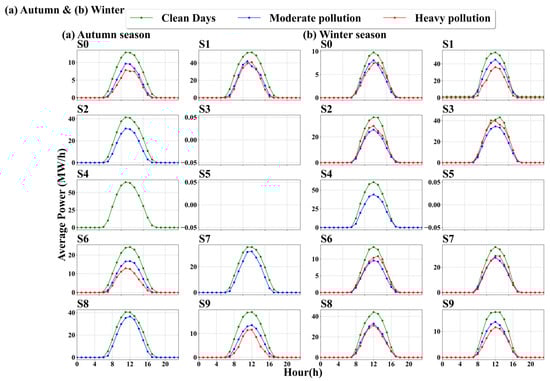
Figure 6.
Diurnal variations in photovoltaic output during autumn and winter under different air quality levels. (a) Autumn season showing longer daylight hours with wider power generation curves, optimal performance under clean weather conditions, and moderate pollution impact on PV output. (b) Winter season demonstrating shortened daylight hours with narrower power curves, reduced overall power levels, and significantly enhanced pollution effects with substantial power reduction during heavy pollution episodes. Lines represent different pollution levels—clean days (green), moderate pollution (blue), and heavy pollution (red). Gaps indicate missing data for specific pollution conditions at certain stations.
Overall, as pollution levels rise, photovoltaic power output at all stations shows a clear decline, especially during noon peak hours, where the adverse effects of pollution on generation are most pronounced. This underscores the detrimental impact of PM2.5 on photovoltaic system performance, resulting in significant energy output reductions.
3.3. Machine Learning-Based Assessment of Air Pollution Effects on PV Performance
To evaluate the influence of air pollution—specifically fine particulate matter (PM2.5)—on the accuracy and stability of PV power forecasting, six machine learning models (SVR, RF, DT, AdaBoost, KNN, and BP) were trained and tested across ten monitoring sites. For each site, the dataset was split into a training set (80%) and a testing set (20%). All performance metrics and visualizations presented in this section are derived exclusively from the testing subset to objectively assess the models’ generalization capability under real-world conditions. S0 was selected as a representative case for in-depth analysis due to its balanced combination of data completeness, seasonal continuity, and spatial representativeness. While it does not exhibit the absolute minimum of missing data, it maintains a high temporal resolution with consistent observations across all four seasons, as shown in Figure 4. Unlike some peripheral sites that exhibit substantial seasonal gaps or concentrated missing intervals, S0 avoids long-term outages and presents a near-continuous time series of hourly PV power records, ensuring modeling reliability. Furthermore, its central geographic location within Hebei Province enhances its statistical representativeness, reducing the influence of localized anomalies in either weather patterns or air pollution. These characteristics make S0 a robust and illustrative benchmark for evaluating model behavior, striking a balance between data quality and regional generalizability.
Figure 7 presents the density scatter plots comparing observed and predicted PV power outputs for the six models at site S0. Overall, all models exhibited a generally linear correlation between predicted and actual values, but their predictive accuracy and distribution characteristics varied notably. RF achieved the most accurate predictions, showing the highest R2 (0.980), the lowest RMSE (0.190 MW), and tightly clustered points along the 1:1 reference line, indicating strong generalization and robustness. KNN and SVR also demonstrated solid performance, with R2 values of 0.970 and 0.969, respectively; KNN produced a more concentrated density but showed increased dispersion in the high-output region, while SVR maintained consistent alignment with slightly more spread in outliers. DT performed moderately (R2 = 0.967), but its outputs revealed clear stepwise clustering—a typical consequence of its discrete partitioning logic that reduces output smoothness. AdaBoost yielded higher errors (RMSE = 0.293 MW) and more variance in prediction spread, suggesting overfitting tendencies and amplified noise under certain intervals. In contrast, BP suffered from severe deviation from the ideal trend, exhibiting the lowest R2 (0.634), the highest RMSE (0.810 MW), and a widely dispersed distribution, reflecting poor model convergence and limited capacity to capture nonlinear dependencies in the dataset.
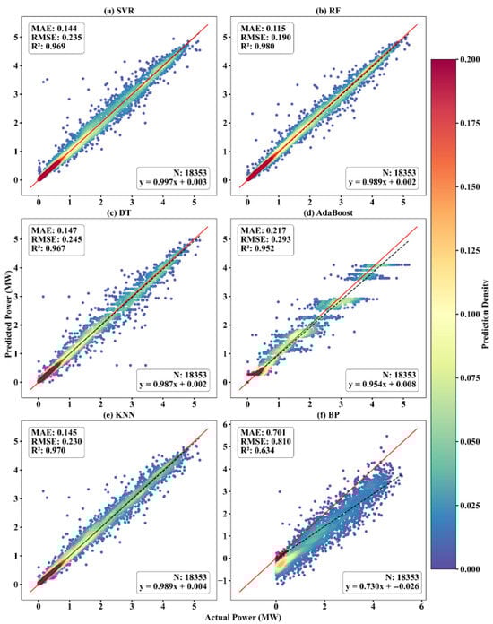
Figure 7.
Comparison of actual and predicted PV power output at Site S0: density scatter plot and model performance metrics.
To extend the evaluation across spatial domains, Figure 8 and Table 3 collectively present the performance of six machine learning models across ten monitoring sites, using boxplots of MSE, MAE, MAPE, and RMSE under both PM2.5-inclusive and PM2.5-free conditions. Among the models, RF exhibited the most favorable and stable performance, achieving the lowest average MAE (0.497 MW) and the highest R2 (0.966) under PM2.5-inclusive conditions, reflecting its strong predictive capacity and robustness to spatial heterogeneity. SVR and KNN followed closely, with similarly low MAE values (0.597 MW and 0.630 MW, respectively) and consistently high R2 scores above 0.92, indicating their effectiveness in capturing regional power generation patterns with minimal sensitivity to PM2.5 inclusion. DT showed moderate performance (MAE = 0.616 MW, R2 = 0.950) but displayed higher variability in MSE and MAPE distributions, suggesting susceptibility to site-specific overfitting due to its partition-based nature. In contrast, BP and AdaBoost exhibited significantly larger prediction errors and reduced model stability. BP yielded the highest MAE (1.039 MW) and a visibly wider spread in RMSE and MAPE values, indicating limited adaptability to spatial and environmental complexity. AdaBoost showed negligible MAE improvement with PM2.5 (from 0.890 MW to 0.888 MW) but produced the highest average MAPE and the largest number of extreme outliers across sites, highlighting its limited robustness in generalized forecasting tasks. These results collectively reinforce the superior spatial generalization ability of RF, SVR, and KNN, particularly when incorporating air pollution factors into PV power prediction models. The inclusion of RMSE and MAPE metrics further validates these findings by revealing RF’s exceptional consistency across different error measures. While RF achieved the lowest MAE (0.497 MW), its superior RMSE (0.851 MW) and MAPE (47.926%) confirm robust performance with minimal sensitivity to outliers and stable percentage errors across varying output ranges. In contrast, BP’s high MAPE (175.156%) and AdaBoost’s extreme MAPE (265.147%) indicate poor reliability under varying atmospheric conditions, supporting their lower ranking in the overall assessment.
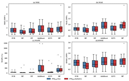
Figure 8.
Boxplot comparison of model performance across ten sites under PM2.5-inclusive and PM2.5-free conditions.
Figure 9 further reinforces the comparative findings by presenting a Taylor diagram that simultaneously integrates RMSE, R2, and STD into a unified visual framework. Among all models, RF is positioned closest to the reference point, indicating the best overall trade-off between error minimization, correlation strength, and output variability alignment. SVR, KNN, and DT form a compact cluster nearby, reflecting similarly strong predictive performance and consistent variance matching. AdaBoost shows moderate deviation from the optimal zone, suggesting reduced precision under certain scenarios. In contrast, BP appears farthest from the reference point, with lower R2, higher RMSE, and greater divergence in STD, confirming its weaker generalization capability. Collectively, the diagram visually confirms the superior robustness and predictive reliability of RF, SVR, and KNN in PV power forecasting.
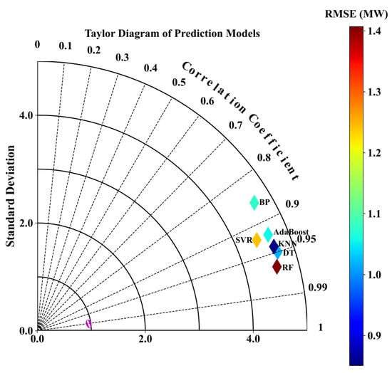
Figure 9.
Taylor diagram of model performance in PV power prediction.
Overall, the results indicate that models such as RF, SVR, and KNN generally exhibit stronger predictive performance across different environmental conditions. While the inclusion of PM2.5 did not lead to pronounced improvements in average metrics, it was associated with modest reductions in prediction errors and enhanced output stability in most cases. These observations suggest that PM2.5 may offer supplementary value in improving model robustness under polluted conditions, although its overall impact appears to be limited and model-dependent.
3.4. Stacking Framework for Enhanced Predictive Accuracy
Stacking is an ensemble modeling technique designed to enhance predictive accuracy by integrating multiple algorithms trained on the same dataset. This approach, known as “stacked generalization”, was proposed by Wolpert in 1992 [56]. It functions by assessing the performance of base classifiers against independent or bootstrapped reference datasets. In a stacking framework, various models are combined to produce a more reliable prediction or classification result. Figure 3 illustrates the fundamental principles of stacking, showcasing how different algorithms can be synergistically merged to capitalize on their respective strengths and achieve improved overall performance. Leveraging the principles of the stacking framework, we implemented this method to improve the accuracy of PV power forecasts. The stacking model consolidates multiple base algorithms, each trained on the same dataset, to capture diverse patterns and insights. A meta-model then integrates the outputs from these various algorithms, effectively addressing the inherent variability in their predictions. This collaborative approach enhances the robustness and reliability of PV power forecasts, ensuring more precise estimations under different conditions. In this section, we focus on the implementation of the stacking framework utilizing six machine learning models previously discussed in Section 2.2.2. The models, referred to by their abbreviations—SVR, RF, DT, AdaBoost, KNN, and BP—were organized into five base learners and one meta-learner, resulting in six combinations, designated as Combination 1 to Combination 6. The input variables and evaluation metrics consistent with previous analyses were employed for training.
The stacking framework was applied to enhance PV power prediction by combining six base learners into six distinct configurations (Comb 1–Comb 6), each evaluated under PM2.5-inclusive and PM2.5-free conditions. As shown in Table 4, Comb 6 achieved the best overall performance, recording the lowest MAE (0.479 MW) and the highest R2 (0.967) under PM2.5-inclusive settings. Comb 1 and Comb 5 followed closely, with MAE values of 0.476 MW and 0.496 MW, respectively, and equally strong R2 scores (0.965). In contrast, Comb 4 produced the highest MAE (0.685 MW) and the lowest R2 (0.955), indicating weaker generalization across spatial sites. The differences in performance across combinations highlight the importance of selecting appropriate model ensembles. These results underscore the effectiveness of stacking in integrating complementary patterns from individual learners and generating more accurate and stable predictions, particularly when PM2.5 information is incorporated.
Table 4.
Performance evaluation of stacking models: comprehensive analysis of MAE, RMSE, MAPE, and R2 metrics under PM2.5 conditions.
To further illustrate this advantage, Figure 10 compares the MAE and R2 values of all models under both PM2.5-inclusive and PM2.5-free conditions. The Figure 10a shows the MAE distribution, where stacking models—particularly Comb 1 through Comb 6—consistently outperform single models, with Comb 6 achieving the lowest overall error. The Figure 10b presents R2 values (ranging from 0.8 to 1.0), where stacking combinations exhibit a consistently higher correlation with observed outputs than individual learners. This comparative visualization clearly demonstrates that stacking not only improves accuracy but also enhances the reliability and uniformity of model performance across diverse environmental conditions.
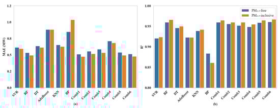
Figure 10.
Performance comparison of individual and stacking-based models under PM2.5-inclusive and PM2.5-free conditions. (a) Mean absolute error (MAE); (b) coefficient of determination (R2). Stacking combinations (Comb 1–Comb 6) generally outperform single models.
When compared with the six single-model baselines presented in Section 3.3 and Table 3, the advantage of stacking becomes more evident. The best-performing individual model, RF, achieved a PM2.5-inclusive MAE of 0.497 MW and R2 of 0.966, while the top stacking combination, Comb 6, further reduced the MAE to 0.479 MW and improved R2 to 0.967. Other strong configurations, such as Comb 1 and Comb 5, also consistently outperformed individual models like SVR, KNN, and DT across both metrics. Notably, even mid-performing ensembles like Comb 2 and Comb 3 remained competitive with or superior to most single models, underscoring the robustness of the stacking strategy. These results confirm that the ensemble integration not only improves average performance but also mitigates specific model weaknesses, such as BP’s overfitting or AdaBoost’s instability. The comprehensive evaluation using four metrics reveals that stacking benefits extend beyond simple MAE improvement. For instance, Comb 6’s superior RMSE (0.832 MW) and MAPE (41.035%) compared to the best individual model RF (RMSE = 0.851 MW, MAPE = 47.926%) demonstrate enhanced robustness and more consistent percentage errors across different PV output levels.
The inclusion of PM2.5 as an input variable also had a consistently positive impact across all stacking configurations. Every combination exhibited a reduction in MAE and a slight increase in R2 when PM2.5 was incorporated. For instance, Comb 1’s MAE decreased from 0.512 MW to 0.476 MW, while R2 rose from 0.960 to 0.965. Similarly, Comb 5 experienced an MAE reduction from 0.542 MW to 0.496 MW and a gain of 0.6 percentage points in R2. Although the absolute increases in R2 were modest, the uniform improvement in MAE across all combinations suggests that PM2.5 contributes valuable explanatory power, especially under variable pollution conditions.
In summary, the application of stacking models significantly enhances the predictive accuracy of PV power forecasting and exhibits greater effectiveness when PM2.5 is considered. The multi-metric evaluation framework confirms these conclusions across different error perspectives, with stacking models showing consistent superiority in RMSE and MAPE alongside traditional metrics. These findings highlight the importance of incorporating air pollution indicators like PM2.5 into future predictive frameworks to improve model performance and support more informed energy management decisions.
4. Discussion
This study demonstrates the critical role of PM2.5 pollution in affecting photovoltaic (PV) power generation accuracy and the potential of machine learning, particularly stacking ensemble methods, in enhancing prediction performance. Our findings confirm that air quality variables, especially PM2.5, should not be overlooked when modeling PV outputs, as they significantly influence radiation components such as GHI and DHI through scattering and absorption processes—consistent with the conclusions drawn in studies by Son et al. [8], Song et al. [15], and Sun et al. [16].
Among individual models, RF exhibited the best overall performance, with an MAE of 0.497 MW and R2 of 0.966 when PM2.5 was included. Its robustness and high accuracy can be attributed to its ensemble nature and ability to capture complex nonlinear relationships. However, the stacking framework—especially Combination 6—further improved prediction accuracy, achieving an MAE of 0.479 and R2 of 0.967. While the margin of improvement may appear moderate numerically, the stacking approach demonstrated more consistent performance across spatially heterogeneous sites, indicating superior generalizability. Notably, RF’s performance approached that of the stacking model, suggesting that in environments with high data quality and feature richness, RF alone may be a cost-effective alternative to more complex ensemble frameworks. The comparative analysis also highlights that models like BP and AdaBoost, which are more sensitive to noise and feature dimensionality, performed less stably under PM2.5-influenced conditions. This further justifies the adoption of hybrid ensemble strategies that mitigate the limitations of individual learners. Recent advances in photovoltaic forecasting research continue to validate the effectiveness of ensemble approaches. Mohanasundaram and Rangaswamy (2025) demonstrated that machine learning techniques, particularly when optimized with advanced algorithms, significantly enhance prediction accuracy in solar energy forecasting, achieving superior performance compared to traditional methods [57]. Recent work published in scientific reports further validates these findings, with comprehensive machine learning evaluations for photovoltaic systems demonstrating that ensemble approaches consistently achieve superior performance compared to individual algorithms, particularly when incorporating environmental variables [58]. This further confirms our conclusions regarding the effectiveness of stacking ensemble approaches.
An important finding of our study is the distinction between linear correlation strength and actual predictive impact. While preliminary correlation analysis indicated weak linear relationships between PM2.5 and PV output, our machine learning results demonstrate that PM2.5 inclusion consistently improves model performance across all algorithms through complex, nonlinear mechanisms that traditional correlation analysis cannot capture. This finding reveals that PM2.5, despite appearing as a weak influencing factor in conventional linear analysis, actually exerts meaningful effects on PV systems through nonlinear pathways. This highlights the value of data-driven approaches in capturing these complex environmental interactions that may be overlooked by simple linear analysis methods. Future research incorporating advanced feature importance methods such as SHAP values or permutation importance would provide more comprehensive insights into these complex relationships and enable better quantification of the relative contributions of all meteorological variables.
Our findings are based on Hebei Province’s specific continental pollution context, which may limit direct applicability to regions with different aerosol characteristics. Future research should prioritize several key directions to enhance our understanding of pollution–PV interactions. Multi-regional validation studies across diverse environments (coastal, desert, tropical, high-altitude) and multi-year analysis across different pollution profiles would strengthen the generalizability of our findings and capture spatiotemporal variability in environmental conditions. Additionally, integrating physical radiative transfer models with machine learning approaches could provide deeper mechanistic insights into aerosol–radiation–PV interactions, while expanding the analysis to include co-pollutants (e.g., NO2, O3) would enable more comprehensive assessment of air quality impacts on renewable energy systems. The importance of accurate solar forecasting has been further emphasized by recent research demonstrating that probabilistic forecasting models can significantly enhance grid reliability and renewable energy integration. Contemporary studies continue to advance the field through innovative approaches that address the challenges of renewable energy variability and improve the operational efficiency of photovoltaic systems.
5. Conclusions
This study conducted a comprehensive investigation of PM2.5 impacts on photovoltaic power generation across Hebei Province through the systematic analysis of data from 10 monitoring stations spanning a complete annual cycle (July 2018–June 2019). We implemented six machine learning algorithms (SVR, RF, DT, AdaBoost, KNN, and BP) and developed an innovative stacking ensemble framework to capture the complex nonlinear relationships between atmospheric pollution and PV performance. Our methodology integrated high-resolution PM2.5 datasets with comprehensive meteorological variables to quantify pollution effects across diverse environmental conditions.
Our investigation revealed that PV output exhibits pronounced spatiotemporal variations, with seasonal fluctuations reaching 31.8% between spring/summer and autumn/winter periods, and remarkable spatial disparities showing up to five-fold differences across regional locations. We demonstrated that PM2.5 pollution exerts substantial impacts on PV performance, with severe pollution episodes causing up to a 48.2% reduction in power output compared to clear atmospheric conditions. The developed stacking ensemble framework achieved exceptional predictive accuracy (MAE = 0.479 MW, R2 = 0.967), significantly outperforming individual models while consistently demonstrating that PM2.5 inclusion enhances forecasting performance across most algorithms.
Assessing our achievements against the three established research objectives: Objective 1 (analyzing spatiotemporal characteristics) was successfully completed, providing comprehensive documentation of regional PV performance patterns with quantified seasonal and spatial variations across the study domain. Objective 2 (quantifying PM2.5 impacts) was effectively accomplished, establishing measurable relationships between PM2.5 concentrations and PV performance and documenting significant output reductions during severe pollution episodes. Objective 3 (developing enhanced prediction framework) was satisfactorily achieved, creating a functional ensemble methodology that demonstrated improved performance compared to individual models and confirming the utility of incorporating atmospheric pollution variables in PV forecasting frameworks.
These findings underscore the importance of aerosol–radiation interactions in PV forecasting. The developed methodological framework offers a robust approach for assessing air quality impacts on solar energy output, contributing to improved atmospheric environment research. This work supports more accurate forecasting models, which can aid in mitigating the effects of air pollution on renewable energy generation and inform policy strategies for sustainable energy management.
Supplementary Materials
The following supporting information can be downloaded at: https://www.mdpi.com/article/10.3390/en18154195/s1, Table S1. Candidate hyperparameter values used for grid search in model training. Table S2. Optimal Hyperparameter Configurations and Training Set Performance for Different Models at Site S0. Table S3. Optimal Hyperparameter Configurations and Training Set Performance for Different Models at Site S1. Table S4. Optimal Hyperparameter Configurations and Training Set Performance for Different Models at Site S2. Table S5. Optimal Hyperparameter Configurations and Training Set Performance for Different Models at Site S3. Table S6. Optimal Hyperparameter Configurations and Training Set Performance for Different Models at Site S4. Table S7. Optimal Hyperparameter Configurations and Training Set Performance for Different Models at Site S5. Table S8. Optimal Hyperparameter Configurations and Training Set Performance for Different Models at Site S6. Table S9. Optimal Hyperparameter Configurations and Training Set Performance for Different Models at Site S7. Table S10. Optimal Hyperparameter Configurations and Training Set Performance for Different Models at Site S8. Table S11. Optimal Hyperparameter Configurations and Training Set Performance for Different Models at Site S9.
Author Contributions
A.H.: writing—review and editing, writing—original draft, visualization, validation, software, methodology, investigation, formal analysis, data curation, conceptualization. Z.D.: writing—review and editing, supervision, resources, project administration, funding acquisition. Y.Z.: writing—review and editing, supervision, resources, project administration, funding acquisition. Z.H.: writing—review and editing, validation, software, methodology, data curation. T.J.: writing—review and editing, supervision, resources, project administration, funding acquisition. X.Y.: writing—review and editing, supervision, resources, project administration, funding acquisition. All authors have read and agreed to the published version of the manuscript.
Funding
This research was funded by the China Meteorological Administration Aerosol-Cloud and Precipitation Key Laboratory (No. KDW2401), China Meteorological Administration Xiong’an Atmospheric Boundary Layer Key Laboratory (No. 2023LABL-B14), the Startup Foundation in Nantong University (No. 135423612053), and the College Students’ Innovation and Entrepreneurship Training Project (No. 2025207).
Institutional Review Board Statement
Not applicable.
Informed Consent Statement
Not applicable.
Data Availability Statement
The PVOD dataset used in this study can be freely downloaded from GitHub at https://github.com/yaotc/PVODataset, accessed on 1 April 2024. The 30 m spatial resolution digital elevation map data used in Figure 1 were provided by the Geospatial Data Cloud site, Computer Network Information Center, Chinese Academy of Sciences (http://www.gscloud.cn), accessed on 5 April 2024. The ChinaHighPM2.5 dataset is available at https://zenodo.org/records/6398971, accessed on 12 May 2024.
Conflicts of Interest
The authors declare no conflict of interest.
Abbreviations
The following abbreviations are used in this manuscript:
| AdaBoost | Adaptive Boosting |
| ANN | Artificial Neural Network |
| BP | Backpropagation Neural Network |
| CHAP | ChinaHighAirPollutants |
| CV-R2 | Cross-Validation Coefficient of Determination |
| DHI | Diffuse Horizontal Irradiance |
| DT | Decision Tree |
| GHI | Global Horizontal Irradiance |
| KNN | K-Nearest Neighbors |
| LMD | Local Measurement Data |
| MAE | Mean Absolute Error |
| MAPE | Mean Absolute Percentage Error |
| MSE | Mean Squared Error |
| NWP | Numerical Weather Prediction |
| P | Atmospheric Pressure |
| PM2.5 | Particulate Matter with diameter ≤ 2.5 micrometers |
| PV | Photovoltaic |
| PVOD | Photovoltaic Output Dataset |
| R2 | Coefficient of Determination |
| RBF | Radial Basis Function |
| RF | Random Forest |
| RMSE | Root Mean Square Error |
| STD | Standard Deviation |
| SVM | Support Vector Machine |
| SVR | Support Vector Regression |
| T | Temperature |
| WD | Wind Direction |
| WS | Wind Speed |
References
- Zhang, D.; Li, Y.; Chin, K.-S. Photovoltaic technology assessment based on cumulative prospect theory and hybrid information from sustainable perspective. Sustain. Energy Technol. Assess. 2022, 52, 102116. [Google Scholar] [CrossRef]
- Kabir, E.; Kumar, P.; Kumar, S.; Adelodun, A.A.; Kim, K.-H. Solar energy: Potential and future prospects. Renew. Sustain. Energy Rev. 2018, 82, 894–900. [Google Scholar] [CrossRef]
- Hernandez, R.R.; Armstrong, A.; Burney, J.; Ryan, G.; Moore-O’Leary, K.; Diédhiou, I.; Grodsky, S.M.; Saul-Gershenz, L.; Davis, R.; Macknick, J. Techno–ecological synergies of solar energy for global sustainability. Nat. Sustain. 2019, 2, 560–568. [Google Scholar] [CrossRef]
- Queisser, H.J.; Werner, J.H. Principles and technology of photovoltaic energy conversion. In Proceedings of the 4th International Conference on Solid-State and IC Technology, Beijing, China, 24–28 October 1995; pp. 146–150. [Google Scholar]
- Yao, T.; Wang, J.; Wu, H.; Zhang, P.; Li, S.; Wang, Y.; Chi, X.; Shi, M. A photovoltaic power output dataset: Multi-source photovoltaic power output dataset with Python toolkit. Sol. Energy 2021, 230, 122–130. [Google Scholar] [CrossRef]
- Benghanem, M.; Mellit, A.; Alamri, S.N. ANN-based modelling and estimation of daily global solar radiation data: A case study. Energy Convers. Manag. 2009, 50, 1644–1655. [Google Scholar] [CrossRef]
- Gueymard, C.A.; Ruiz-Arias, J.A. Extensive worldwide validation and climate sensitivity analysis of direct irradiance predictions from 1-min global irradiance. Sol. Energy 2016, 128, 1–30. [Google Scholar] [CrossRef]
- Son, J.; Jeong, S.; Park, H.; Park, C.-E. The effect of particulate matter on solar photovoltaic power generation over the Republic of Korea. Environ. Res. Lett. 2020, 15, 84004. [Google Scholar] [CrossRef]
- Kumar, P.; Vogel, H.; Bruckert, J.; Muth, L.J.; Hoshyaripour, G.A. MieAI: A neural network for calculating optical properties of internally mixed aerosol in atmospheric models. npj Clim. Atmos. Sci. 2024, 7, 110. [Google Scholar] [CrossRef]
- Samset, B.H.; Stjern, C.W.; Andrews, E.; Kahn, R.A.; Myhre, G.; Schulz, M.; Schuster, G.L. Aerosol Absorption: Progress Towards Global and Regional Constraints. Curr. Clim. Change Rep. 2018, 4, 65–83. [Google Scholar] [CrossRef] [PubMed]
- Zhang, X.; Chen, S.; Kang, L.; Yuan, T.; Luo, Y.; Alam, K.; Li, J.; He, Y.; Bi, H.; Zhao, D. Direct Radiative Forcing Induced by Light-Absorbing Aerosols in Different Climate Regions Over East Asia. J. Geophys. Res. Atmos. 2020, 125, e2019JD032228. [Google Scholar] [CrossRef]
- Yang, Y.; Mou, S.; Wang, H.; Wang, P.; Li, B.; Liao, H. Global source apportionment of aerosols into major emission regions and sectors over 1850–2017. Atmos. Chem. Phys. 2024, 24, 6509–6523. [Google Scholar] [CrossRef]
- Ghosh, S.; Dey, S.; Ganguly, D.; Roy, S.B.; Bali, K. Cleaner air would enhance India’s annual solar energy production by 6–28 TWh. Environ. Res. Lett. 2022, 17, 54007. [Google Scholar] [CrossRef]
- Ghosh, S.; Ganguly, D.; Dey, S.; Chowdhury, S.G. Future photovoltaic potential in India: Navigating the interplay between air pollution control and climate change mitigation. Environ. Res. Lett. 2024, 19, 124030. [Google Scholar] [CrossRef]
- Song, Z.; Wang, M.; Yang, H. Quantification of the Impact of Fine Particulate Matter on Solar Energy Resources and Energy Performance of Different Photovoltaic Technologies. ACS Environ. Au 2022, 2, 275–286. [Google Scholar] [CrossRef] [PubMed]
- Sun, K.; Lu, L.; Jiang, Y.; Wang, Y.; Zhou, K.; He, Z. Integrated effects of PM2.5 deposition, module surface conditions and nanocoatings on solar PV surface glass transmittance. Renew. Sustain. Energy Rev. 2018, 82, 4107–4120. [Google Scholar] [CrossRef]
- Kim, M.J. Air Pollution and Solar Photovoltaic Power Generation: Evidence from South Korea. Energy Econ. 2024, 139, 107924. [Google Scholar] [CrossRef]
- Bao, Z.; Shi, R.; Huang, Y.; Song, X. Photovoltaic generation potential and developmental suitability in southern Hebei. Energy Rep. 2023, 9, 795–805. [Google Scholar] [CrossRef]
- Wang, P.; Zhang, S.; Pu, Y.; Cao, S.; Zhang, Y. Estimation of photovoltaic power generation potential in 2020 and 2030 using land resource changes: An empirical study from China. Energy 2021, 219, 119611. [Google Scholar] [CrossRef]
- Liang, L.; Chen, Z.; Chen, S.; Zheng, X. Evaluation of Site Suitability for Photovoltaic Power Plants in the Beijing-Tianjin-Hebei Region of China Using a Combined Weighting Method. Land 2024, 13, 40. [Google Scholar] [CrossRef]
- Wu, W.; Zhang, M.; Ding, Y. Exploring the effect of economic and environment factors on PM2.5 concentration: A case study of the Beijing-Tianjin-Hebei region. J. Environ. Manag. 2020, 268, 110703. [Google Scholar] [CrossRef] [PubMed]
- He, C.; Huang, G.; Liu, L.; Li, Y.; Zhai, M.; Cao, R. Assessment and offset of the adverse effects induced by PM2.5 from coal-fired power plants in China. J. Clean. Prod. 2021, 286, 125397. [Google Scholar] [CrossRef]
- Huang, T.; Yu, Y.; Wei, Y.; Wang, H.; Huang, W.; Chen, X. Spatial-seasonal characteristics and critical impact factors of PM2.5 concentration in the Beijing-Tianjin-Hebei urban agglomeration. PLoS ONE 2018, 13, e0201364. [Google Scholar] [CrossRef]
- Zhou, J.; Yin, T.; Tian, J. Research on the impact of Beijing-Tianjin-Hebei electric power and thermal power industry on haze pollution. Energy Rep. 2022, 8, 1698–1710. [Google Scholar] [CrossRef]
- Mayer, M.J.; Gróf, G. Extensive comparison of physical models for photovoltaic power forecasting. Appl. Energy 2021, 283, 116239. [Google Scholar] [CrossRef]
- Moreira, M.; Balestrassi, P.; Paiva, A.; Ribeiro, P.; Bonatto, B. Design of experiments using artificial neural network ensemble for photovoltaic generation forecasting. Renew. Sustain. Energy Rev. 2021, 135, 110450. [Google Scholar] [CrossRef]
- Sobri, S.; Koohi-Kamali, S.; Rahim, N.A. Solar photovoltaic generation forecasting methods: A review. Energy Convers. Manag. 2018, 156, 459–497. [Google Scholar] [CrossRef]
- Zheng, Z.; Chen, Y.; Huo, M.; Zhao, B. An overview: The development of prediction technology of wind and photovoltaic power generation. Energy Procedia 2011, 12, 601–608. [Google Scholar] [CrossRef]
- Luo, X.; Zhang, D.; Zhu, X. Deep learning based forecasting of photovoltaic power generation by incorporating domain knowledge. Energy 2021, 225, 120240. [Google Scholar] [CrossRef]
- Yadav, A.K.; Chandel, S.S. Solar radiation prediction using Artificial Neural Network techniques: A review. Renew. Sustain. Energy Rev. 2014, 33, 772–781. [Google Scholar] [CrossRef]
- Zendehboudi, A.; Baseer, M.A.; Saidur, R. Application of support vector machine models for forecasting solar and wind energy resources: A review. J. Clean. Prod. 2018, 199, 272–285. [Google Scholar] [CrossRef]
- Simon, S.M.; Glaum, P.; Valdovinos, F.S. Interpreting random forest analysis of ecological models to move from prediction to explanation. Sci. Rep. 2023, 13, 3881. [Google Scholar] [CrossRef]
- Wang, Y.; Tian, S.; Zhang, P. Novel spatio-temporal attention causal convolutional neural network for multi-site PM2.5 prediction. Front. Environ. Sci. 2024, 12, 1408370. [Google Scholar] [CrossRef]
- Mfetoum, I.M.; Ngoh, S.K.; Molu, R.J.J.; Nde Kenfack, B.F.; Onguene, R.; Naoussi, S.R.D.; Tamba, J.G.; Bajaj, M.; Berhanu, M. A multilayer perceptron neural network approach for optimizing solar irradiance forecasting in Central Africa with meteorological insights. Sci. Rep. 2024, 14, 3572. [Google Scholar]
- Feng, Y.; Hao, W.; Li, H.; Cui, N.; Gong, D.; Gao, L. Machine learning models to quantify and map daily global solar radiation and photovoltaic power. Renew. Sustain. Energy Rev. 2020, 118, 109393. [Google Scholar] [CrossRef]
- Odhiambo, M.R.O.; Abbas, A.; Wang, X.; Mutinda, G. Solar Energy Potential in the Yangtze River Delta Region-A GIS-Based Assessment. Energies 2021, 14, 143. [Google Scholar] [CrossRef]
- Wu, W.; Zhang, T.; Xie, X.; Huang, Z. Regional low carbon development pathways for the Yangtze River Delta region in China. Energy Policy 2021, 151, 112172. [Google Scholar] [CrossRef]
- Xu, C.; Xie, D.; Gu, C.; Zhao, P.; Wang, X.; Wang, Y. Sustainable development pathways for energies in Yangtze River Delta urban agglomeration. Sci. Rep. 2023, 13, 18135. [Google Scholar] [CrossRef] [PubMed]
- Xu, J.; Zhao, C.; Wang, F.; Yang, G. Industrial decarbonisation oriented distributed renewable generation towards wastewater treatment sector: Case from the Yangtze River Delta region in China. Energy 2022, 256, 124562. [Google Scholar] [CrossRef]
- Peng, Y.; Azadi, H.; Yang, L.; Scheffran, J.; Jiang, P. Assessing the Siting Potential of Low-Carbon Energy Power Plants in the Yangtze River Delta: A GIS-Based Approach. Energies 2022, 15, 2167. [Google Scholar] [CrossRef]
- Liang, M.S.; Huang, G.H.; Chen, J.P.; Li, Y.P. Energy-water-carbon nexus system planning: A case study of Yangtze River Delta urban agglomeration, China. Appl. Energy 2022, 308, 118144. [Google Scholar] [CrossRef]
- Wei, J.; Li, Z.; Lyapustin, A.; Sun, L.; Peng, Y.; Xue, W.; Su, T.; Cribb, M. Reconstructing 1-km-resolution high-quality PM2.5 data records from 2000 to 2018 in China: Spatiotemporal variations and policy implications. Remote Sens. Environ. 2021, 252, 112136. [Google Scholar] [CrossRef]
- Wei, J.; Li, Z.; Cribb, M.; Huang, W.; Xue, W.; Sun, L.; Guo, J.; Peng, Y.; Li, J.; Lyapustin, A.; et al. Improved 1 km resolution PM2.5 estimates across China using enhanced space–time extremely randomized trees. Atmos. Chem. Phys. 2020, 20, 3273–3289. [Google Scholar] [CrossRef]
- Liu, C.; Gao, Z.; Li, Y.; Gao, C.Y.; Su, Z.; Zhang, X. Surface Energy Budget Observed for Winter Wheat in the North China Plain During a Fog-Haze Event. Bound.-Layer Meteorol. 2019, 170, 489–505. [Google Scholar] [CrossRef]
- Sun, Y.; Zhang, J.; Zhang, Y. Adaboost algorithm combined multiple random forest models (Adaboost-RF) is employed for fluid prediction using well logging data. Phys. Fluids 2024, 36, 16602. [Google Scholar] [CrossRef]
- Essamlali, I.; Nhaila, H.; El Khaili, M. Supervised Machine Learning Approaches for Predicting Key Pollutants and for the Sustainable Enhancement of Urban Air Quality: A Systematic Review. Sustainability 2024, 16, 976. [Google Scholar] [CrossRef]
- Benti, N.E.; Chaka, M.D.; Semie, A.G. Forecasting Renewable Energy Generation with Machine Learning and Deep Learning: Current Advances and Future Prospects. Sustainability 2023, 15, 7087. [Google Scholar] [CrossRef]
- Vasisht, M.S.; Srinivasan, J.; Ramasesha, S.K. Performance of solar photovoltaic installations: Effect of seasonal variations. Sol. Energy 2016, 131, 39–46. [Google Scholar] [CrossRef]
- Li, X.; Wagner, F.; Peng, W.; Yang, J.; Mauzerall, D.L. Reduction of solar photovoltaic resources due to air pollution in China. Proc. Natl. Acad. Sci. USA 2017, 114, 11867–11872. [Google Scholar] [CrossRef]
- Song, Z.; Liu, J.; Yang, H. Air pollution and soiling implications for solar photovoltaic power generation: A comprehensive review. Appl. Energy 2021, 298, 117247. [Google Scholar] [CrossRef]
- Song, Z.; Cao, S.; Yang, H. Quantifying the air pollution impacts on solar photovoltaic capacity factors and potential benefits of pollution control for the solar sector in China. Appl. Energy 2024, 365, 123261. [Google Scholar] [CrossRef]
- Labordena, M.; Neubauer, D.; Folini, D.; Patt, A.; Lilliestam, J. Blue skies over China: The effect of pollution-control on solar power generation and revenues. PLoS ONE 2018, 13, e0207028. [Google Scholar] [CrossRef] [PubMed]
- Chiabrando, R.; Fabrizio, E.; Garnero, G. The territorial and landscape impacts of photovoltaic systems: Definition of impacts and assessment of the glare risk. Renew. Sustain. Energy Rev. 2009, 13, 2441–2451. [Google Scholar] [CrossRef]
- Zhang, L.; Zhang, Y.; Yi, X.; Yang, Y.; Zhao, M.; Zhou, J. Seasonal variations of the impact of urban aerosol pollution on distributed solar photovoltaic generation of nine megacities in China. Urban Clim. 2020, 34, 100723. [Google Scholar] [CrossRef]
- Luo, Y.; Zhao, T.; Yang, Y.; Zong, L.; Kumar, K.R.; Wang, H.; Meng, K.; Zhang, L.; Lu, S.; Xin, Y. Seasonal changes in the recent decline of combined high PM2.5 and O3 pollution and associated chemical and meteorological drivers in the Beijing–Tianjin–Hebei region, China. Sci. Total Environ. 2022, 838, 156312. [Google Scholar] [CrossRef]
- Wolpert, D.H. Stacked generalization. Neural Netw. 1992, 5, 241–259. [Google Scholar] [CrossRef]
- Mohanasundaram, V.; Rangaswamy, B. Photovoltaic solar energy prediction using the seasonal-trend decomposition layer and ASOA optimized LSTM neural network model. Sci. Rep. 2025, 15, 4032. [Google Scholar] [CrossRef] [PubMed]
- Hamad, S.A.; Ghalib, M.A.; Munshi, A.; Alotaibi, M.; Ebied, M.A. Evaluating machine learning models comprehensively for predicting maximum power from photovoltaic systems. Sci. Rep. 2025, 15, 10750. [Google Scholar] [CrossRef]
Disclaimer/Publisher’s Note: The statements, opinions and data contained in all publications are solely those of the individual author(s) and contributor(s) and not of MDPI and/or the editor(s). MDPI and/or the editor(s) disclaim responsibility for any injury to people or property resulting from any ideas, methods, instructions or products referred to in the content. |
© 2025 by the authors. Licensee MDPI, Basel, Switzerland. This article is an open access article distributed under the terms and conditions of the Creative Commons Attribution (CC BY) license (https://creativecommons.org/licenses/by/4.0/).