Ultra-Short-Term Photovoltaic Power Prediction Based on Predictable Component Reconstruction and Spatiotemporal Heterogeneous Graph Neural Networks

Abstract

Ultra-short-term PV power prediction (USTPVPP) results provide a basis for the development of intra-day rolling power generation plans. However, due to the feature information and the unpredictability of meteorology, the current ultra-short-term PV power prediction accuracy improvement still faces technical challenges. In this paper, we propose a combined prediction framework that takes into account the reconfiguration of the predictable components of PV stations and the spatiotemporal heterogeneous maps. A circuit singular spectral decomposition (CISSD) intrinsic predictable component extraction method is adopted to obtain specific frequency components in sensitive meteorological variables, a mechanism based on radiation characteristics and PV power trend predictable component extraction and reconstruction is proposed to enhance power predictability, and a spatiotemporal heterogeneous graph neural network (STHGNN) combined with a Non-stationary Transformer (Ns-Transformer) combination architecture to achieve joint prediction for different PV components. The proposed method is applied to a PV power plant in Gansu, China, and the results show that the prediction method based on the proposed combined spatio-temporal heterogeneous graph neural network model combined with the proposed predictable component extraction achieves an average reduction of 6.50% in the RMSE, an average reduction of 2.50% in the MAE, and an average improvement of 11.93% in the R² over the direct prediction method, respectively.

1. Introduction

1.1. Background

USTPVPP provides important guidance for the development of intra-day optimal scheduling and rolling generation plans for power systems. Common USTPVPPs are mainly based on statistical [1], physical [2], and artificial intelligence [3] methods, which usually use historical power as the main input information to build time series prediction models. In order to further improve the PV power prediction accuracy, a large number of studies have introduced numerical weather prediction into the PV power prediction process [4]. Influenced by the chaotic effect of weather systems, frequent occurrence of extreme weather [5], numerical prediction bias [6], and the degree of extraction of predictable feature information [7], the improvement in the ultra-short-term prediction performance of PV power is still faced with technical bottlenecks.

The main reason for the occurrence of PV power prediction bias is the meteorological variability due to the chaotic effect of weather systems, especially the frequent occurrence of uncertainties such as cloud evolution and precipitation. Therefore, means such as extracting the predictability components included in the PV power or correcting the radiation will help to improve the PV power prediction accuracy [8,9,10]. With the development of graph neural network (GNN) technology [11], single-node prediction of PV power has gradually transitioned towards the direction of multi-node joint prediction, and a large number of studies have been conducted on the application of GNNs to the prediction of PV cluster power as well as the evolutionary speculation of the cloud paths [12,13], which consider PV cluster as a network, and individual PV stations as nodes, and describe the relationship between nodes through the neighbor matrix describes the correlation between nodes to extract sensitive information that incorporates spatiotemporal correlation, which helps to improve the power prediction accuracy of individual PV stations in PV cluster to achieve effective cluster prediction. The development of GNN structure provides a new idea for the heterogeneous connectivity of the PV stations [14]: Applying different graph structures to the same network can realize multiple graph relations to capture the correlations in the network, which can further enhance the extraction of such fusion features and achieve unexpected prediction results [15].

1.2. Related Research

In order to enhance the PV power prediction accuracy, existing studies mainly focus on feature extraction and sensitive feature screening, scenario clustering, model optimization and improvement, and prediction correction. In the input link of the prediction model, many researchers, in order to enhance the sensitivity of input features, usually use feature selection, feature extraction, and scenario clustering to improve the model’s learning ability of the input information. Ref. [16] proposes a sensitive input feature screening method based on a genetic algorithm (GA) optimization mechanism for acquiring key features. Ref. [17] proposes a sensitive variable screening method based on maximum information coefficient, Ref. [18] proposes a feature importance analysis method based on random forest (RF), and Ref. [19] proposes a feature selection method based on temporal importance model explanation and utilizes the interpretable outputs to screen globally important features. Some other studies have used correlation coefficients [20], mutual information [21], etc., to construct the correlation between input features and output features to obtain important features. More studies focus on using model feature extraction to obtain key features for model training. Ref. [22] proposes a sensitive feature extraction method based on a convolutional neural network architecture, similarly Refs. [23,24]. Ref. [25] proposes a temporal convolution network (TCN) based feature extraction method to obtain temporal features, and Ref. [26] combines TCN and gated recurrent unit (GRU) modules to extract temporal features from input features. Similarly, there are some multi-node feature fusion methods based on GNN for PV power prediction [27,28]. Considering the volatility of PV sequences, some studies have used multiple decomposition methods to reconstruct the predictable components of the power or meteorological sequences in order to enhance the predictability of the PV sequences effectively. Ref. [29] uses empirical modal decomposition (EMD) to obtain the smooth component in the power series. Ref. [30] proposes a predictable component reconstruction strategy based on ensemble empirical modal decomposition (EEMD), similarly improved complete ensemble EMD with adaptive noise (ICEEMDAN) [31], complete ensemble EMD with adaptive noise (CEEMDAN) [32], and variational mode decomposition (VMD) [33]. Even some studies combine multiple decomposition methods and use the combined decomposition mechanism to further extract the predictable components of the power series [34]. In order to improve the learning ability of the model for different types of data, a large number of studies also focus on the refined scenario division. Ref. [35] proposes a k-means++ clustering model for similar day screening, Ref. [36] screens similar days based on Pearson’s correlation coefficient, and Ref. [37] proposes a similar day screening mechanism based on fuzzy C-means clustering (Fc-means). Ref. [38] classifies weather types into desirable and undesirable meteorological processes and models them separately. Whether it is based on feature selection, feature extraction, or refined modeling of scene division, it can effectively improve the PV power prediction accuracy.

In the model training session, a large number of researchers focus on model optimization and improvement, trying to obtain high-precision PV power prediction results by improving model performance. Ref. [39] proposes a PV power prediction method based on artificial bee colony optimization depth model, Ref. [40] proposes a prediction method based on sparrow search algorithm (SSA) to optimize the bidirectional long and short-term memory networks (BILSTM) model, Ref. [41] proposes a prediction method based on gray wolf optimization algorithm (GWO) to optimize prediction model, and similarly, there are also optimization methods such as secretary bird optimization algorithm (SBOA) [42], improved particle swarm optimization algorithm (IPSO) [43] and improved genetic algorithm (IGA) [44]. There are also some studies that use combined prediction models for model performance enhancement, Ref. [45] proposes a prediction architecture based on convolutional neural network (CNN) combined with BILSTM, Ref. [46] proposes a combined prediction model based on CNN and bidirectional gated recurrent unit (BIGRU), and there are some other studies that use the combined architecture of Transformer and BILSTM [47] or BIGRU [48] for extracting the temporal features of PV sequences. The model optimization session adjusts the model hyperparameters to enhance the learning ability and generalization of the model, while the model improvement process integrates the advantages of different models or modules, which can further enhance the extraction and learning effect of the model on PV features. In the model output link, in order to minimize the impact of prediction errors on the results, many studies have used the error correction method to improve the PV power prediction accuracy. Ref. [49] performed wavelet decomposition of PV power prediction error and used artificial neural network to predict different components to realize error prediction and power correction, Ref. [50] used LSTM model to predict PV power prediction error in order to correct the power, Ref. [51] used the method of time series prediction to predict the error based on extreme learning machine (ELM), and Ref. [52] used similar error correction methods to improve the prediction results.

In summary, the current research on PV power prediction is usually based on the strategies of feature screening, feature extraction, model optimization and improvement, and correction of prediction results to improve its prediction performance. However, feature selection and screening usually require high data quality, and cannot effectively improve the prediction performance when the data quality is low, while modeling strategies based on scenario division and model optimization usually require large modeling costs and are difficult to strike a balance between prediction accuracy and modeling costs, and strategies based on error correction usually use temporal extrapolation to improve the modeling accuracy, but are usually applicable to short time scales and are difficult to apply to longer time scales. While error–correction approaches typically employ time series extrapolation to enhance model precision, they are generally suited for shorter forecasting horizons and prove less effective for extended periods. Furthermore, enhancing photovoltaic power prediction accuracy by focusing on the extractable predictable relationship between meteorological factors and power output remains an underexplored area. To bridge this gap, this study introduces a PV power forecasting approach centered on predictable feature extraction and a spatiotemporal heterogeneous graph neural network. This method aims to isolate the most pertinent PV predictable components and boost prediction accuracy through an integrated spatiotemporal heterogeneous graph neural network architecture. The key innovations presented herein include:

(1)

A novel predictable component reconstruction method based on ETO-CISSD is proposed for extracting predictable key components in PV meteorological features.

(2)

An optimal component evaluation function based on correlation coefficient and ranking entropy weighting is proposed to guide CISSD to obtain the most efficient decomposition results.

(3)

Propose a meteorological-power predictable correlation component reconstruction method to obtain the predictable components in PV sequences.

(4)

A combined prediction model based on a spatiotemporal heterogeneous map neural network combined with Ns-Transformer is proposed for the prediction of multiple components of PV power.

The rest of the paper consists of Section 2: Methodology, Section 3: Case study, Section 4: Analysis and discussion, and Section 5: Conclusions.

2. Methodology

Enhancing photovoltaic power forecasting precision is constrained by meteorological instability and inaccuracies in numerical weather prediction (NWP). To address this limitation, we propose a novel predictable element reconstruction technique termed CISSD, which efficiently extracts forecastable components with reduced computational overhead. This method decomposes NWP irradiance data into distinct predictable elements. Furthermore, an ETO-driven optimization mechanism is developed to mitigate hyperparameter sensitivity during decomposition, thereby refining CISSD’s parameter configuration. Based on the extraction of predictable components of irradiance, the historical measured irradiance and PV power are reconstructed to obtain fully predictable PV components by associating them with predictable components. A combined learning framework based on a spatiotemporal heterogeneous graph neural network and Ns-Transformer is proposed to achieve the prediction of predictable and fluctuating components of PV.

2.1. Predictable Component Extraction Based on CISSD

Circulant singular spectrum decomposition [53] is an improved decomposition method based on singular spectral decomposition (SSD). Distinguished from SSD, CISSD is able to obtain the components of the ideal frequency with high efficiency in the decomposition process, and its whole process is still divided into four steps:

(1)

Embedding: this step is the same as SSD.

(2)

Decomposition: compute the cyclic matrix $S_C$, find the eigenvalue ${\tilde{\lambda }}_k$ of $S_C$, and associate the kth eigenvalue and the corresponding eigenvector with the frequency $w_k={\displaystyle \frac{k-1}{L}},k=1,\dots ,L$. Where $S_C$ can be calculated by the element $\widehat{c_m}$ corresponding to the following relation:

$$\widehat{c_m}={\displaystyle \frac{L-m}{L}}{\widehat{\gamma }}_m+{\displaystyle \frac{m}{L}}{\widehat{\gamma }}_{L-m},m=0,\dots ,L-1$$

(1)

where ${\widehat{\gamma }}_m$ can be expressed as follows:

$${\widehat{\gamma }}_m={\displaystyle \frac{1}{T-m}}{\displaystyle {\sum }_{t=1}^{T-m}{x}_t{x}_{t+m}}$$

(2)

(3)

Grouping: taking into account the symmetry of the power spectral density, it is obtained that ${\tilde{\lambda }}_k={\tilde{\lambda }}_{L+2-k}$. Their corresponding eigenvectors are complex; therefore, they are conjugate complex pairs, $u_k=u_{L+2-k}^{*}$. $u^{*}$ denotes the complex conjugate $u$ of the vectors, and $u_k^{\prime }X$ and $u_{L+2-k}^{\prime }X$ correspond to the same harmonic period, which are transformed into pairs of real eigenvectors in order to compute the associated components. In order to form the elementary matrices, it is necessary to first form the groups of the two elements $B_k=\left\{k,L+2-k\right\},k=2,\dots ,M,B_1=\left\{1\right\}$ and $B_{{\displaystyle \frac{t}{2}}+1}=\left\{{\displaystyle \frac{L}{2}}+1\right\}$. Secondly, we compute the fundamental matrix in terms of the frequency $X_{B_k}$ as a sum of the two fundamental matrices $X_k$ and $X_{L+2-k}$, related to the eigenvalues ${\tilde{\lambda }}_k$ and ${\tilde{\lambda }}_{L+2-k}$ and the frequency $w_k={\displaystyle \frac{k-1}{L}}$.

$$X_{B_k}=X_k+X_{L+2-k}=u_k{u}_k^{H}X+u_{L+2-k}{u}_{L+2-k}^{H}X=\left(u_k{u}_k^H+u_k^{*}{u}_k^{\prime }\right)X=2\left(R_{u_k}{R}_{u_k}^{\prime }+I_{u_k}{I}_{u_k}^{\prime }\right)X$$

(3)

where $R_{u_k}$ denotes the real part of $u_k$, $I_{u_k}$ denotes its imaginary part, and $u^H$ denotes the conjugate transpose of a vector $u$. Note that the matrix $X_{B_k},k=1,\dots ,L$ is real.

(4)

Reconstruction: this step is the same as SSD. Based on the reconstruction link $m$, forecast irradiance sequence components with different frequencies are obtained:

$$DIMF={\left(\begin{array}{cccc}im{f}_{11}& im{f}_{12}& \dots & im{f}_{1n}\\ im{f}_{21}& im{f}_{22}& \dots & im{f}_{2n}\\ \dots & \dots & \dots & \dots \\ im{f}_{m1}& im{f}_{m2}& \dots & im{f}_{mn}\end{array}\right)}^{m\times n}$$

(4)

where $im{f}_{mn}$ denotes the value at the nth time point of the mth component after decomposition, $m$ denotes the number of sequences after decomposition, and $n$ denotes the length of the sequence.

To mitigate CISSD hyperparameter sensitivity during decomposition, we implement the Exponential Triangular Optimization (ETO) algorithm [54]. This approach optimizes the window length parameter of CISSD, enhancing decomposition efficacy. Subsequent to optimization, predictable elements and high-frequency oscillatory components are extracted. The fitness function governing ETO integrates permutation entropy (Pe) [55,56,57] and correlation metrics, where minimized Pe in low-frequency predictable components coupled with maximized correlation to the source signal indicates: (1) reduced component complexity, (2) elevated predictability, and (3) preserved signal integrity. Therefore, the fitness function is constructed as the summation of the modified correlation coefficient and Pe between predictable components and the original signal, formalized as follows:

$$Fit=\left(1-R^{*}\left(IP,SC\right)\right)+Pe\left(IP\right)$$

(5)

$$Pe\left(IP\right)=-{\displaystyle {\sum }_{i=1}^{n}I{P}_i\ln \left(I{P}_i\right)}$$

(6)

$$R^{*}\left(IP,SC\right)=\left(1+R\left(IP,SC\right)\right)/2$$

(7)

$$R\left(IP,SC\right)={\displaystyle \frac{\left({\displaystyle {\sum }_{i=1}^n\left(I{P}_i-\overline{IP}\right)\cdot \left(S{C}_i-\overline{SC}\right)}\right)}{\left(\sqrt{{\displaystyle {\sum }_{i=1}^n{\left(I{P}_i-\overline{IP}\right)}^2}}\cdot \sqrt{{\displaystyle {\sum }_{i=1}^n{\left(S{C}_i-\overline{SC}\right)}^2}}\right)}}$$

(8)

where, $Fit$ denotes the fitness function, $SC$ and $IP$ denote the original sequence and the decomposed predictable component sequence, respectively, $\overline{SC}$ and $\overline{IP}$ denote the mean value of the original sequence and the decomposed predictable component sequence, respectively, $R^{*}\left(\right)$ denotes the correlation coefficient modification operator, $Pe\left(\right)$ denotes the formula of Pe, $n$ denotes the length of the sequence, and $R$ denotes the correlation coefficient.

2.2. Reconstruction of the Predictable Component of the Correlation of Weather/Power

The trend component and high-frequency fluctuation component of the NWP irradiance sequence are obtained on the basis of Equation (4), and generally after the decomposition, the first component can be used as the trend component of the irradiance sequence, which is used in this paper as the predictable component for the historical real irradiance sequence as well as the basis for the reconstruction of the predictable component of the PV power sequence. It is assumed that the predictable component sequence of the forecasted irradiance series is $Ps={\left[p{s}_1,\dots ,p{s}_n\right]}^{1\times n}$, and its fluctuation component sequence is $Ws={\left[w{s}_1,\dots ,w{s}_n\right]}^{1\times n}$, whose sum represents the sequence before the original decomposition. Based on this, the predictable component for the historical PV power sequence can be obtained with the following expression:

$$Po\left(i\right)=\left[Ps\left(i\right)\cdot {\displaystyle {\sum }_{i=1}^{n}Hp\left(i\right)}\right]/{\displaystyle {\sum }_{i=1}^{n}Ps\left(i\right)}$$

(9)

where $Po\left(i\right)$, $Ps\left(i\right)$, and $Hp\left(i\right)$ denote the ith reconstructed historical predictable PV power point, the predictable component of the forecasted irradiance sequence, and the PV power point before reconstruction, respectively. The construction method is mainly to take the product of the point-by-point ratio of the predictable component of the forecasted irradiance sequence to the total irradiance and the historical total PV power sum as the reconstructed PV power predictable component, and since the reconstruction process fully satisfies the linear relationship, the PV power predictable component is able to be predicted completely and accurately. Therefore, the fluctuation component of power can be expressed as follows:

$$Wo\left(i\right)=Hp\left(i\right)-Po\left(i\right)$$

(10)

where $Wo\left(i\right)$ denotes the ith reconstructed historical fluctuating PV power point.

As the predictable component of power is extracted, the remaining fluctuation component needs to be predicted based on another part of the fluctuation input feature, this paper introduces the historical measured irradiance sequence as the source of input information, constructs the predictable and fluctuation components based on historical measured irradiance based on predictable input $Ps$, and predicts the fluctuation component of PV power based on the method of time series prediction. Since the predictable component of NWP irradiance can completely and effectively predict the predictable component of PV power, it is necessary to use the same method to extract the predictable component in the sequence of measured irradiance and use the remaining component as the basis for the prediction of the fluctuation component of PV power. As a result, in this paper, the predictable component of the historical measured irradiance series is directly replaced by the NWP irradiance predictable component with the following expression:

$$P_{Ms}\left(i\right)=Ps\left(i\right)$$

(11)

where $P_{Ms}\left(i\right)$ denotes the predictable component point of the ith reconstructed historical measured irradiance series. On this basis, an expression for the calculation of its fluctuation component can be obtained:

$$W_{Ms}\left(i\right)=Ms\left(i\right)-P_{Ms}\left(i\right)$$

(12)

where $Ms\left(i\right)$ and $W_{Ms}\left(i\right)$ denote the ith reconstructed historical measured irradiance series and its fluctuation component points, respectively.

On this basis, expressions for the prediction relationships for the predictable and unpredictable components can be obtained as follows:

$$\left\{\begin{array}{l}Ps\left(i\right)\Rightarrow Po\left(i\right)\\ W_{Ms}\left(i-16\right)+Wo\left(i-16\right)\Rightarrow Wo\left(i\right)\end{array}\right.$$

(13)

where $A\Rightarrow B$ indicates that $A$ is used as the model input to predict $B$. Therefore, the predictable component of NWP irradiance is used as the input to predict the predictable component of PV power in the prediction stage, and the fluctuation component of historical measured irradiance and the historical fluctuation component of PV power are used as the inputs to predict the PV power fluctuation component in the time period to be predicted.

In order to enhance the predictability of the fluctuation component, this paper adopts CISSD to decompose both $W_{Ms}$ as well as $Wo$, and constructs the prediction model for different components; thus, Equation (13) can be expressed as follows:

$$\left\{\begin{array}{l}Ps\left(i\right)\Rightarrow Po\left(i\right)\\ IM{F}_{W_{Ms}}\left(i-16,j\right)+IM{F}_{Wo}\left(i-16,j\right)\Rightarrow Wo\left(i,j\right)\end{array}\right.$$

(14)

where $IM{F}_{W_{Ms}}\left(i,j\right)$, as well as $IM{F}_{Wo}\left(i,j\right)$, denote the ith value corresponding to the $W_{Ms}$ and $Wo$ components of the jth decomposition, respectively.

2.3. Combined Multicomponent Prediction Based on STHGNN-Ns-Transformer

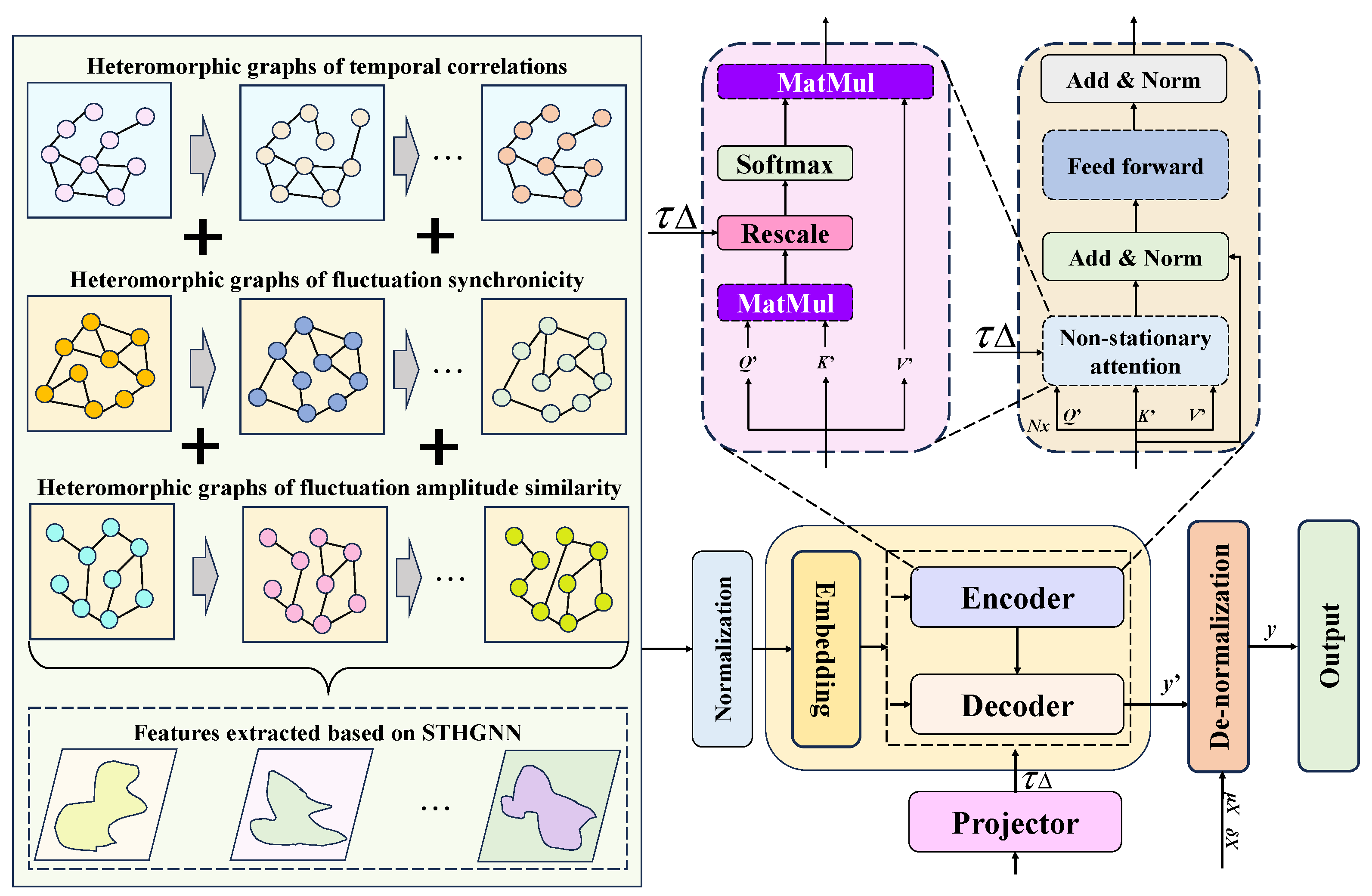
This paper specifies the prediction input and output mechanisms for the PV power predictable component as well as the fluctuation component. In this regard, a combined framework based on Ns-Transformer [58] and a heterogeneous spatiotemporal graph neural network is proposed for the prediction of the PV power predictable component as well as multiple fluctuation sub-components. This combination aims to effectively capture the dynamic spatial dependencies between nodes and the temporal dependencies of the nodes’ own evolution over time in complex spatiotemporal data, which is the key to handling the PV power prediction task. This combined model is mainly used to learn a mapping function F that is capable of predicting PV power based on a history of T time steps of graph-structured spatiotemporal data X = [X₁, X₂, …, X_t] ∈ R^{N×T×C} (where N is the number of nodes, T is the historical time step, and C is the node feature dimension, as in Figure 1), and predicts that the future T′ time steps of data Y = [Y₁, Y₂, …, Y_t′] ∈ R^{{N×T′×C′}} (C′ may be different from C). The powerful spatial relationship modelling capability of STHGNN is combined with the efficient and flexible temporal dependency modelling capability of Ns-Transformer. Usually adopts a ‘space first, time second’ or ‘space-time interleaved’ architectural strategy.

(1) STHGNN: This paper needs to predict different components of PV power simultaneously and achieve effective prediction of multiple types of components. In the spatial modelling session, the joint prediction of multiple types of components is mainly involved. Hence, in order to improve the learning ability of the model, this paper uses a heterogeneous spatiotemporal graph neural network to model this process. The graph convolution is performed independently at each time step t to aggregate the neighbourhood information:

$$H_t^{\left(l\right)}=\sigma \left({\displaystyle {\sum }_{k=0}^{K-1}{\theta }_k^{\left(l\right)}\cdot T_k\left(\tilde{L}\right)\cdot H_t^{\left(l-1\right)}}\right)$$

(15)

where $H_t^{\left(0\right)}$ denotes the input features at time step t, $\tilde{L}$ denotes the scaled graph Laplace matrix, $T_k\left(\tilde{L}\right)$ denotes the Chebyshev polynomials that approximate the spectral domain convolution kernel, ${\theta }_k^{\left(l\right)}$ denotes the learnable parameters, and σ denotes the activation function (e.g., ReLU). Two temporal modules stacked with one spatial module are used to form a spatiotemporal map convolutional layer for spatiotemporal feature extraction. The historical PV predictable component, irradiance predictable component, and fluctuation component are used as inputs to the temporal feature extraction module for temporal convolution, and the weighted adjacency matrix of each PV component is used as input to the spatial feature extraction module for spatial convolution. Each PV component is represented as a node, and the correlation between the nodes is represented by connecting lines with weight values. The PV component at the moment t can be represented by the spatiotemporal graph as follows:

$$G_t=〈V_t,E〉,V_t=\left\{v_{i,t}\right\}\left(i=1,2,3,\dots ,n\right)E=\left\{w_{i,j}\right\}\left(i,j=1,2,3,\dots ,n\right)$$

(16)

where $V_t=\left\{v_{i,t}\right\}$ denotes the set of power generation data of all nodes in the spatiotemporal graph at time t, $E=\left\{w_{i,j}\right\}$ denotes the weighted adjacency matrix of the connecting lines in the spatiotemporal graph, and $w_{i,j}$ denotes the weight coefficient between node $v_i$ and node $v_j$. A graph convolution network is used to extract the spatial features of each node in the PV component topology graph, while a normalised Laplace matrix is used in the spectral domain to define the PV component graph structure as follows:

$$L=I-D^{-{\displaystyle \frac{1}{2}}}E{D}^{{\displaystyle \frac{1}{2}}}$$

(17)

where I denotes the unit matrix, E denotes the weighted adjacency matrix of the PV plant power map structure, and D denotes the degree matrix of the PV plant power map structure.

Eigen-decomposition of the normalised Laplace matrix can be obtained as the matrix consisting of the eigenvectors of $L=U\Lambda U^T,U\in R^{N\times N}$. $\Lambda =\left[\lambda 1,\lambda 2,\dots ,\lambda n\right]$ is the eigenvalue matrix consisting of the eigenvalues of L. Simplifying the arithmetic operation of graph convolution, the graph convolution formula can be obtained as follows:

$$\left(X_m\ast g\right)=U\left(\left(U^{T}g\right)\odot \left(U^T{X}_m\right)\right)$$

(18)

where $X_m$ denotes the graph convolution neural network input, i.e., the output of the time convolution module, g denotes the convolution kernel, ☉ denotes the Hadamard product. Using $g\theta$ = $U^{T}g$ as the convolution kernel and $\theta \in R^{N\times N}$, the graph convolution formula is obtained as follows:

$$\left(X_m\ast g\right)=U{g}_{\theta }{U}^T{X}_m$$

(19)

(2) Constructing spatiotemporal heterogeneous graphs: in order to effectively capture the evolutionary relationships such as correlation, fluctuation synchrony, and fluctuation magnitude among different PV power components, on the basis of STHGNN, this paper adopts a multi-type heterogeneous maps neural network to model the relationships among PV power components. Among them, the spatiotemporal graph of STHGNN is a ternary group:

$$g=\left(C,W,B\right)$$

(20)

where $g$ is the heterogeneous spatiotemporal map of the STHGNN, $C={\left\{c_i\right\}}_{i=1}^N$ denotes the correlation adjacency matrix describing the component evolution, $W={\left\{w_i\right\}}_{i=1}^N$ denotes the fluctuation synchronisation adjacency matrix describing the component evolution, and $B={\left\{b_i\right\}}_{i=1}^N$ denotes the size proximity adjacency matrix describing the component evolution.

In order to reasonably characterize the functions of the three kinds of adjacency matrices, this paper adopts different calculation guidelines to describe these connection relationships, respectively. For $C={\left\{c_i\right\}}_{i=1}^N$, this paper adopts the correlation coefficient to calculate the connection relationship in the adjacency matrix, and adopts the correlation strength to quantitatively describe the size of the connection weight, and the calculation formula is as follows:

$$c_{ij}={\displaystyle \frac{{\displaystyle {\sum }_{i=1}^n\left(S_i-\overline{S_i}\right)\left(S_j-\overline{S_j}\right)}}{\sqrt{{\displaystyle {\sum }_{i=1}^n{\left(S_i-\overline{S_i}\right)}^2}}\cdot \sqrt{{\displaystyle {\sum }_{i=1}^n{\left(S_j-\overline{S_j}\right)}^2}}}},i=1,\dots ,N,j=1,\dots ,N$$

(21)

where $c_{ij}$ denotes the weight of the correlation adjacency matrix between the target node $i$ and the reference node $j$, $S_i$ and $S_j$ denote the sequence of the ith target node and the sequence of the jth reference node, respectively, and $N$ denotes the number of system nodes.

In order to describe the synchronisation of fluctuations between nodes, this paper adopts the minimum delay correlation to describe this connectivity relationship. Firstly, the delay correlation matrix between the target node $i$ and reference node $j$ is calculated:

$$c^{\tau }={\left[\begin{array}{cccc}{c}_{11}^{\tau }& c_{12}^{\tau }& \dots & c_{1n}^{\tau }\\ c_{21}^{\tau }& c_{21}^{\tau }& \dots & c_{2n}^{\tau }\\ \dots & \dots & \dots & \dots \\ c_{m1}^{\tau }& c_{m2}^{\tau }& \dots & c_{mn}^{\tau }\end{array}\right]}^{m\times n}$$

(22)

where $c_{ij}^{\tau }$ denotes the correlation between the target node $i$ and reference node $j$ after delaying $\tau$ time steps, and $T^{thr}$ denotes the delay time step threshold. After this calculation, the delay correlation matrix of $T^{thr}$ target nodes $i$ and reference node $j$ can be obtained, and finally, the optimal delay step matrix between the target node $i$ and reference node $j$ can be obtained:

$${\tau }^o={\left[\begin{array}{cccc}{\tau }_{11}^o& {\tau }_{12}^o& \dots & {\tau }_{1n}^o\\ {\tau }_{21}^o& {\tau }_{21}^o& \dots & {\tau }_{2n}^o\\ \dots & \dots & \dots & \dots \\ {\tau }_{m1}^o& {\tau }_{m2}^o& \dots & {\tau }_{mn}^o\end{array}\right]}^{\tau },\tau =1,\dots ,T^{thr}$$

(23)

where ${\tau }_{ij}^o$ denotes the optimal delay step matrix between the target node $i$ and the reference node $j$. When the delay step is larger, it means that the fluctuation synchronisation between the nodes is weaker and vice versa, based on which the neighbourhood matrix weight $W_{ij}$ between the target node $i$ and reference node $j$ can be calculated as follows.

$$W={\left[\begin{array}{cccc}1/{\tau }_{11}^o& 1/{\tau }_{12}^o& \dots & 1/{\tau }_{1n}^o\\ 1/{\tau }_{21}^o& 1/{\tau }_{21}^o& \dots & 1/{\tau }_{2n}^o\\ \dots & \dots & \dots & \dots \\ 1/{\tau }_{m1}^o& 1/{\tau }_{m2}^o& \dots & 1/{\tau }_{mn}^o\end{array}\right]}^{m\times n}$$

(24)

On this basis, in order to obtain the correlation of the size of fluctuations between the describing nodes, this paper adopts the average absolute amplitude difference to describe, when the average absolute amplitude difference between the target node i and the reference node j is larger, it means that the degree of fluctuation between the two components of the similarity of the degree of fluctuation is lower, and vice versa, it is larger, and its calculation method is as follows:

$$B_{ij}=l/{\displaystyle \sum _{k=1}^l\left|S_i\left(k\right)-S_j\left(k\right)\right|}$$

(25)

$$B={\left[\begin{array}{cccc}{B}_{11}& B_{12}& \dots & B_{1n}\\ B_{21}& B_{22}& \dots & B_{2n}\\ \dots & \dots & \dots & \dots \\ B_{m1}& B_{m2}& \dots & B_{mn}\end{array}\right]}^{m\times n}$$

(26)

where $B_{ij}$ denotes the fluctuation size similarity between the target node i and the reference node j, $l$ denotes the length of the reference node and the target node used to compute the similarity, and $S_i\left(k\right)$ and $S_j\left(k\right)$ denote the kth value of the target node i and the reference node j, respectively. The final computationally obtained heterogeneous graph matrix describing the correlation, fluctuation, synchronisation, and size similarity between nodes g.

(3) Ns-Transformer: In order to further integrate the spatiotemporal features of STHGNN, this paper mainly adopts a non-smooth Transformer to further extract the spatiotemporal features and effectively extracts the non-smooth information from these features to achieve the high-precision prediction of PV fluctuation power. The common Transformer adopts the traditional location coding and ignores the inter-node heterogeneity, while Ns-Transformer learns the unique location coding vector for each node i:

$$S_t^{\left(i\right)}=h_t^{\left(i\right)}+E_t^{\left(i\right)},\begin{array}{c}E\in R^{N\times d_h}\end{array}$$

(27)

where $h_t^{\left(i\right)}$ denotes the feature of node i at time t, which is derived from the output of the STHGNN, and $E_t^{\left(i\right)}$ denotes the trainable parameter, which portrays the intrinsic temporal pattern of node i. Due to the high complexity of the traditional standard self-attention, Ns-Transformer introduces a local window mask, $M\in {\left\{0,-\infty \right\}}^{T\times T}$, and employs a sparse self-attention mechanism to solve this problem as follows:

$$Attention\left(Q,K,V,M\right)=soft\max \left({\displaystyle \frac{QK}{\sqrt{d_h}}}+M\right)V$$

(28)

where $M_{t_i,t_j}=0$, if and only if $\left|i-j\right|\le w$. The complexity is significantly reduced after this operation, supporting long sequence processing to preserve local key dependencies while suppressing noisy associations.

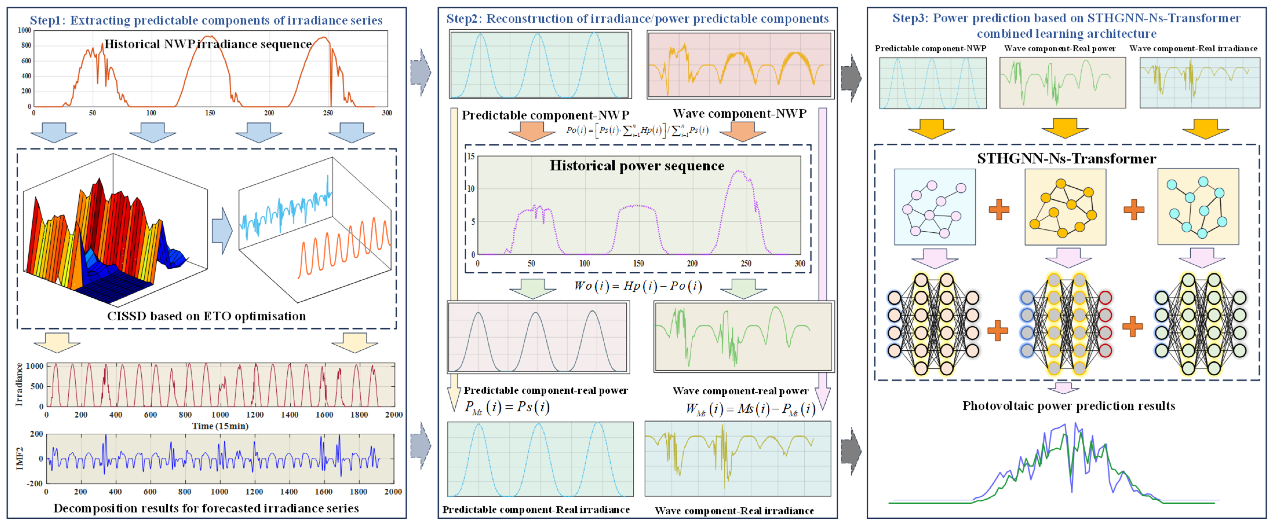
The main research technique framework of this paper is as follows:

(1)

Extraction of predictable components of NWP irradiance sequence: The historical NWP irradiance sequence is decomposed using the CISSD decomposition method based on ETO optimization to extract its predictable components and fluctuation sequence.

(2)

Reconstruction based on historical real irradiance sequence and power sequence: Based on the predictable component of NWP irradiance obtained in step (1), the predictable and fluctuating components of the historical power sequence as well as the predictable and fluctuating components of the historical real irradiance sequence are obtained according to Equations (4)–(14), respectively.

(3)

PV power prediction based on an STHGNN-Ns-Transformer combined architecture: for the PV power components extracted in steps (1) and (2), a combined spatiotemporal heterogeneous graphical neural network combined with Ns-Transformer is used to model the spatiotemporal evolution and dependency between different components, and ultimately achieve high-precision prediction of PV power. The overall research framework is shown in Figure 2.

3. Case Study

Validation of the proposed methodology utilizes operational data (2020–2022) from a 100 MW photovoltaic plant in Gansu, China, the input meteorological features are mainly gridded numerical weather forecasting corresponding to the location of the PV stations, including: irradiance, cloudiness, precipitation, etc., and a sequence of historical measured irradiance is also used to correct the forecasting irradiance. The temporal resolution of all these data is 15 min, and the spatial resolution is 3 km × 3 km. The forecasting data are obtained from the National Meteorological Centre of China, and the measured data are obtained from the real-time monitoring data of the corresponding PV stations. In the prediction session, we mainly use the time series information of the forecasting meteorological data at the corresponding grid of the PV stations as the model input to achieve the power prediction. The training set comprises consecutive operational years (2020–2021), with full-year 2022 data reserved for method verification. Prediction accuracy is quantified through three metrics: Root Mean Square Error (RMSE), Mean Absolute Error (MAE), and Coefficient of Determination (R²), formally defined as follows:

$$RMSE=\sqrt{{\displaystyle \frac{1}{n}}\cdot {\displaystyle {\sum }_{i=1}^n{\left(\frac{p_i-p_i^{\prime }}{Cap}\right)}^2}}$$

(29)

$$MAE={\displaystyle \frac{1}{n}}{\displaystyle {\sum }_{i=1}^n\left|\frac{p_i-p_i^{\prime }}{Cap}\right|}$$

(30)

$$R^2={\displaystyle \frac{{\displaystyle {\sum }_{i=1}^n{\left(p_i-\overline{p}\right)}^2}-{\displaystyle {\sum }_{i=1}^n{\left(p_i-p_i^{\prime }\right)}^2}}{{\displaystyle {\sum }_{i=1}^n{\left(p_i-\overline{p}\right)}^2}}}$$

(31)

where $p_i$ represents the ith actual value, $p_i^{\prime }$ represents the ith predicted value, $\overline{p_i}$ represents the mean of the real value, $n$ represents the sequence length, and $Cap$ represents the total installed capacity of the cluster.

3.1. Irradiance Predictable Component Extraction Based on ETO-CISSD

The ETO-optimized CISSD method decomposes historical NWP irradiance sequences to isolate predictable low-frequency constituents and fluctuating elements. Benchmarking against VMD, EMD, CEEMDAN, and ICEEMDAN algorithms evaluates decomposition performance through dual metrics: (1) correlation coefficients quantifying alignment between extracted predictable components and source signals, and (2) Pe describing sequence complexity. To assess trend extraction capability across methods, sub-components from each decomposition technique are cumulatively reconstructed from low to high frequency. This yields superposition components whose Pe values and correlation coefficients relative to the original irradiance data are computed (

Table 1. Correlation coefficients between the decomposed submodules corresponding to different sub-models and the original signal.

Models	1	1–2	1–3	1–4	1–5	1–6	1–7	1–8	1–9
CISSD	0.9838	0.9954	0.9975	0.9983	0.9987	0.9991	0.9994	0.9997	1.0000
VMD	0.0231	0.2896	0.9237	0.9894	0.9948	0.9972	0.9986	0.9994	1.0000
EMD	0.0909	0.2371	0.3215	0.4001	0.4506	0.5839	0.8577	0.9420	1.0000
CEEMDAN	0.2671	0.2795	0.4214	0.9559	0.9895	0.9941	0.9968	0.9984	1.0000
ICEEMDAN	0.2666	0.2801	0.4043	0.9552	0.9895	0.9941	0.9969	0.9984	1.0000

Note: The frequency of the signal sub-components increases from 1 to 9 in order; bold indicates emphasis.

and

Table 2. Pe of the decomposed sub-modal corresponding to different models with the original signal.

Models	1	1–2	1–3	1–4	1–5	1–6	1–7	1–8	1–9
CISSD	0.4422	0.5402	0.6126	0.6733	0.7554	0.7995	0.8423	0.8496	0.9809
VMD	0.5230	0.6093	0.6737	0.7460	0.8134	0.8756	0.9538	0.9704	0.9809
EMD	0.7410	0.7661	0.8459	0.8624	0.8705	0.8825	0.8950	0.9044	0.9809
CEEMDAN	0.4022	0.4194	0.4432	0.4530	0.5055	0.5733	0.6766	0.8062	0.9809
ICEEMDAN	0.4010	0.4177	0.4420	0.4521	0.5046	0.5745	0.6745	0.8008	0.9809

Note: The frequency of the signal sub-components increases from 1 to 9 in order; bold indicates emphasis.

). The correlation coefficient corresponding to the first sub-component of the CISSD-based decomposition reaches 0.9838, which is completely higher than the correlation coefficients corresponding to the rest of the models, and the correlation coefficients corresponding to the CISSD decomposition sequences are the largest as the number of superimposed sub-components increases, and the corresponding correlation coefficients corresponding to this paper’s model are on average higher than those corresponding to the rest of the models for the superpositions of components 1, 1–2, and 1–3 respectively, and 0.8219 and 0.4798, respectively. Although the Pe of the superposition sequence corresponding to each sub-component of the decomposition method proposed in this paper is not the lowest, it is significantly lower than that of most models. In particular, the first sub-component corresponds to the largest correlation coefficient and relatively small Pe, which is in strong contrast to the first sub-component of CEEMDAN and ICEEMDAN. Although the Pe of the superimposed sequence of sub-components after ICEEMDAN decomposition is lower, its correlation coefficient is very low, and the CISSD decomposition mechanism proposed in this paper significantly improves the extraction effect for predictable components. The extraction effect is significantly improved for predictable components using the CISSD decomposition mechanism proposed in this paper.

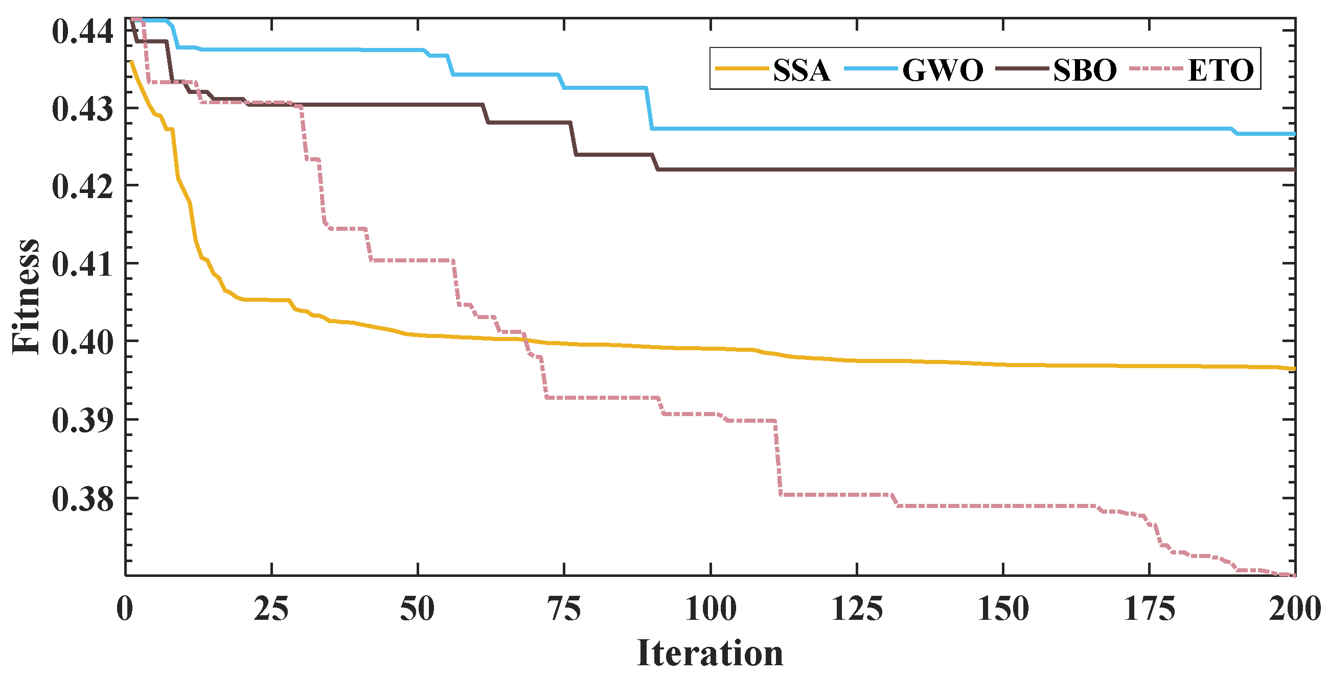
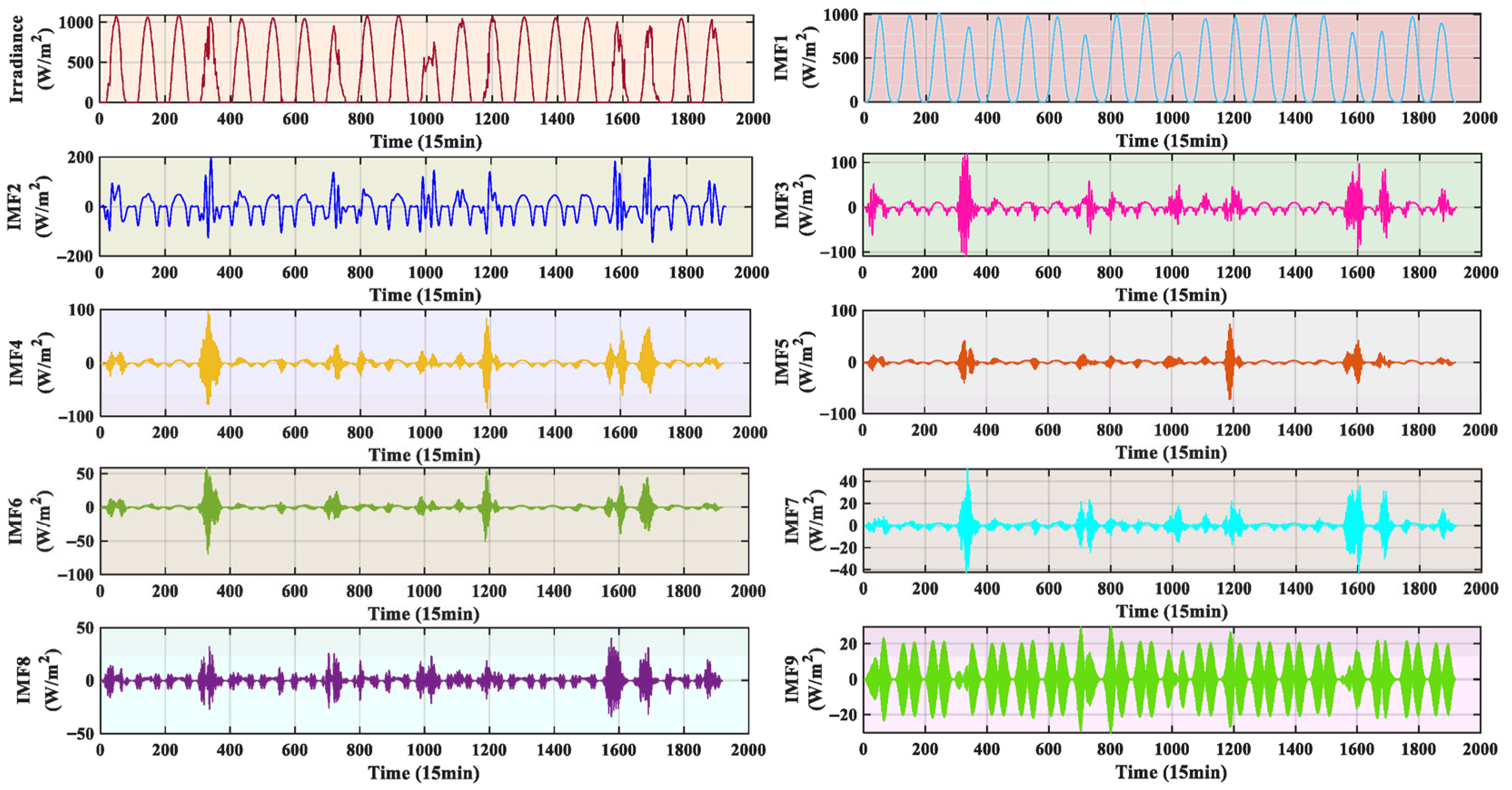
A comparative analysis of optimization efficacy benchmarks ETO against established algorithms (SSA, GWO, SBO). Figure 3 depicts their fitness trajectories during CISSD decomposition under a uniform experimental configuration: population size = 60, maximum iterations = 200. Post-200-iteration convergence is observed across all methods, with ETO demonstrating superior convergence performance—achieving an average fitness reduction of 0.0079 versus alternatives.

Table 3. Optimization results of different optimization algorithms.

Optimization Algorithm	Fitness Value	Time-Consuming (s)	Parameters 1	Parameters 2
SSA	0.3892	120.1416	15	1
GWO	0.3901	132.4515	12	1
SBO	0.4021	125.1783	11	1
ETO	0.3700	136.5425	16	1

Note: Parameters 1 and 2 denote the decomposition window width of CISSD and the parameters related to sequence characteristics, respectively.

documents critical convergence metrics: computational duration, final fitness values, and optimized decomposition parameters. Although ETO incurs longer optimization time, it attains minimal converged fitness and extracts enhanced-predictability components. Figure 4 shows part of the irradiance sequence after CISSD decomposition based on the ETO optimization, which corresponds to a significant correlation between the original signal and the IMF1, while the IMF1 retains most of the information of the original signal and has a significant predictability, and the fluctuating components of the irradiance sequence are shown in the remaining components.

3.2. Irradiance/Power Predictable Component Extraction

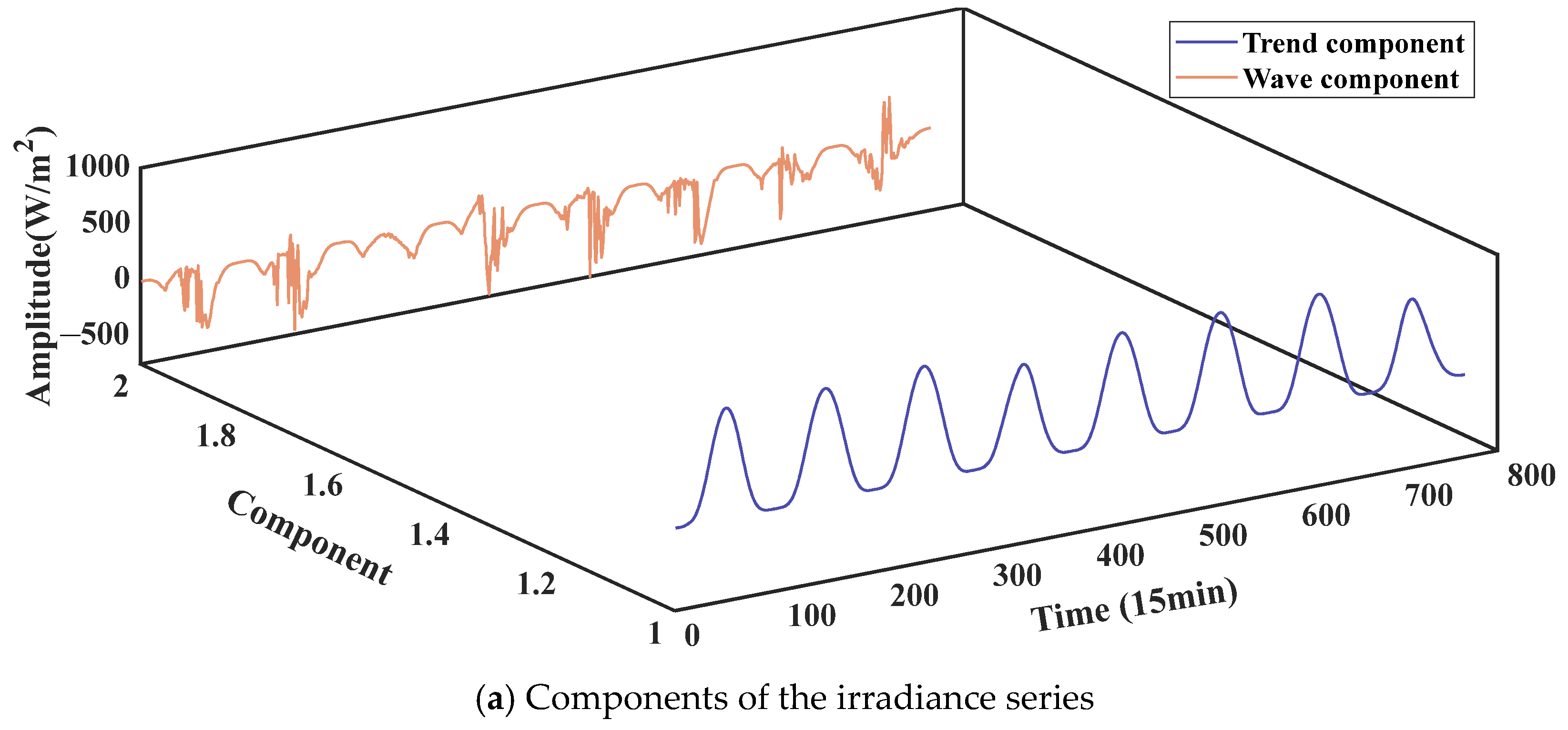
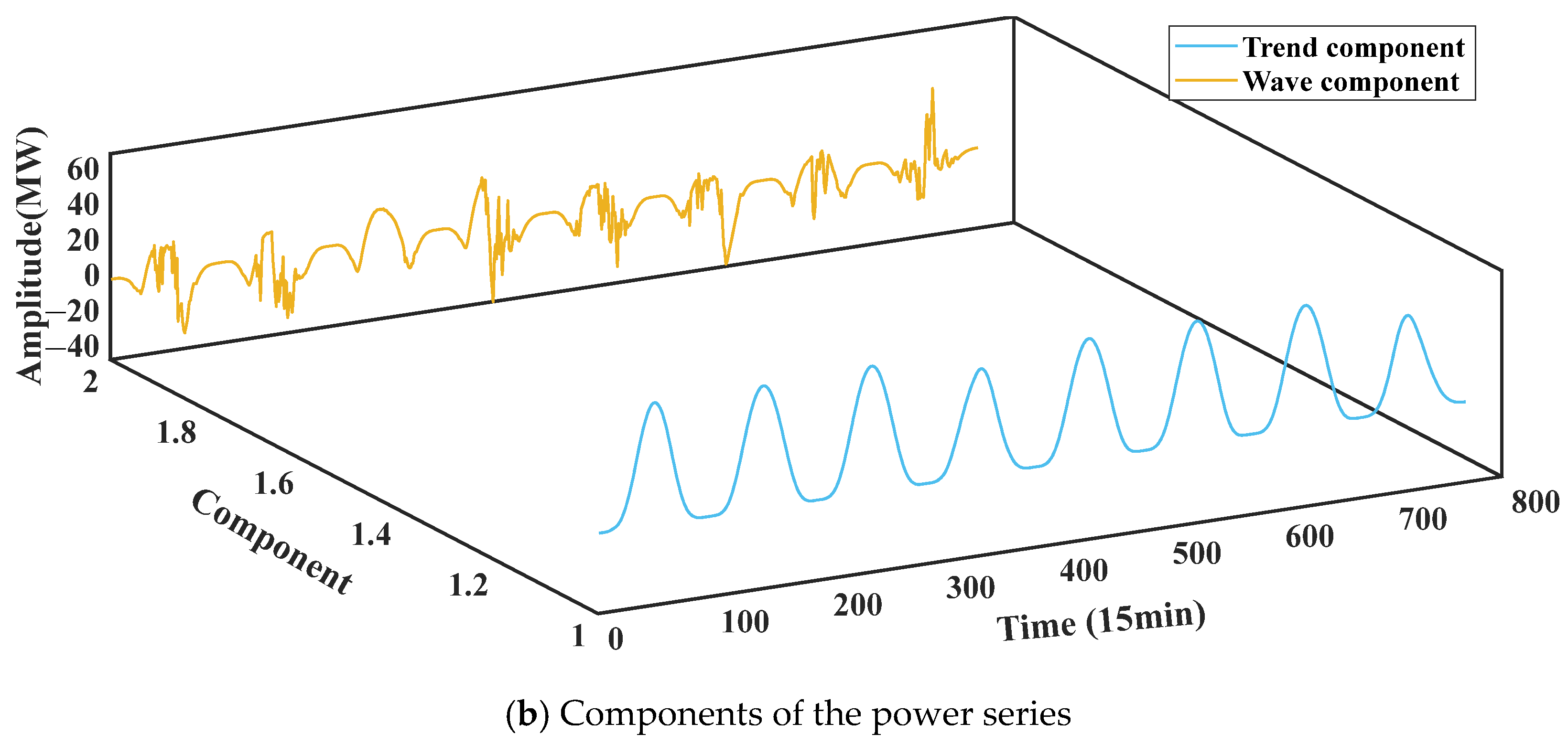
Based on the above decomposition of the NWP irradiance sequence, its IMF Component 1 is extracted as its predictable component, based on which the predictable components of the historical measured irradiance sequence and the PV power sequence are calculated based on Equations (9)–(12) and used for power prediction. Among them, the predictable components of the measured irradiance series are consistent with the predictable components of the NWP irradiance, and the residual components in the measured irradiance series are used as its fluctuation components. Similarly, the predictable and fluctuation components of power were calculated based on Equations (9) and (10), and Figure 5 shows the predictable and fluctuation components of the historical irradiance and PV power sequences, respectively, where the predictable component corresponding to the irradiance sequence differs from that of the power sequence in magnitude, but the trends of their sequences are identical, while the corresponding fluctuation component reflects the meteorological volatility. Although the irradiance fluctuation component and the power fluctuation component are relatively close to each other, they still have differences. During forecasting, the NWP predictable component primarily drives the power predictable element prediction. However, substantial discrepancies between NWP-derived and power fluctuation components preclude effective direct forecasting of power oscillations using NWP fluctuations. Consequently, this work employs time-series extrapolation with field-measured irradiance fluctuations and historical power fluctuations as inputs to project future power oscillatory behavior, thereby achieving precise photovoltaic power forecasting.

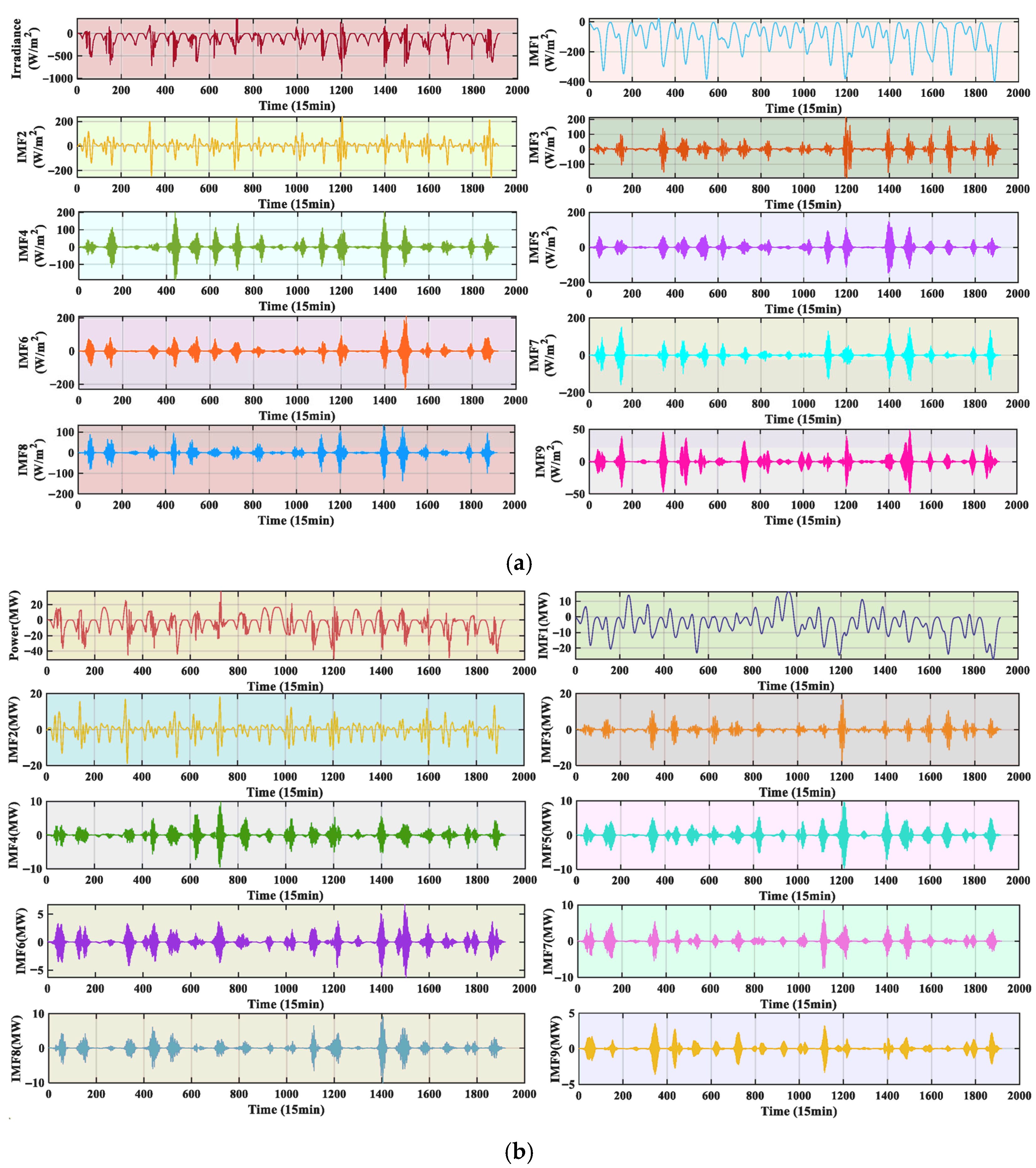
In order to predict the power fluctuation components more effectively, this paper still adopts the CISSD decomposition method to decompose the fluctuation components of irradiance and historical power to obtain the components with different frequencies. Among them, for irradiance and power fluctuation components decomposition, CISSD needs to set the same parameters to ensure that the fluctuation components of historical irradiance and power sequences are obtained with the same number of sub-components. As shown in Figure 6, each component corresponds to a similar sequence trend; the historical values of irradiance and power sequences in each component are used as inputs to predict the power sequences of the same component in future time periods.

3.3. The Combined PV Power Prediction Framework Based on the STHGNN-Ns-Transformer

In Section 3.2, the predictable and fluctuation components of the measured irradiance and power sequences are obtained based on the proposed predictable and fluctuation component extraction method, and the secondary component extraction is carried out for the fluctuation characteristics of the fluctuation components to ensure the effective prediction of the fluctuation components. On this basis, the combined architecture of a spatiotemporal heterogeneous graphical neural network and Ns-Transformer is used for the multicomponent prediction of predictable and fluctuating components. In order to compare the effectiveness of the methods proposed in this paper, the following comparative ablation experiments are proposed:

(1)

Ablation Experiment 1: Compare the prediction performance of different models for PV power using the direct prediction method, comparing the performance of different prediction models, such as BP, ELM, RF, SVM, LSTM, BILSTM, TCN-LSTM, TCN-BILSTM, Transformer, and Ns-Transformer [59,60].

(2)

Ablation experiment 2: Compare the predictability of the method of extracting predictable component in the complete decomposition and in this paper in the above different comparison models. At this time, the ablation Experiment 1 showed a better performance in a certain number of models, as well as STHGNN, STHGNN-Ns-Transformer, as a benchmark model for the experiment.

(3)

Ablation Experiment 3: Compare the prediction performance under the traditional single-node modelling and prediction, multi-node joint prediction, and multi-input and multi-output mechanisms, select certain models with better performance as the benchmark models for the experiments, and at the same time, compare the modelling costs of the different models.

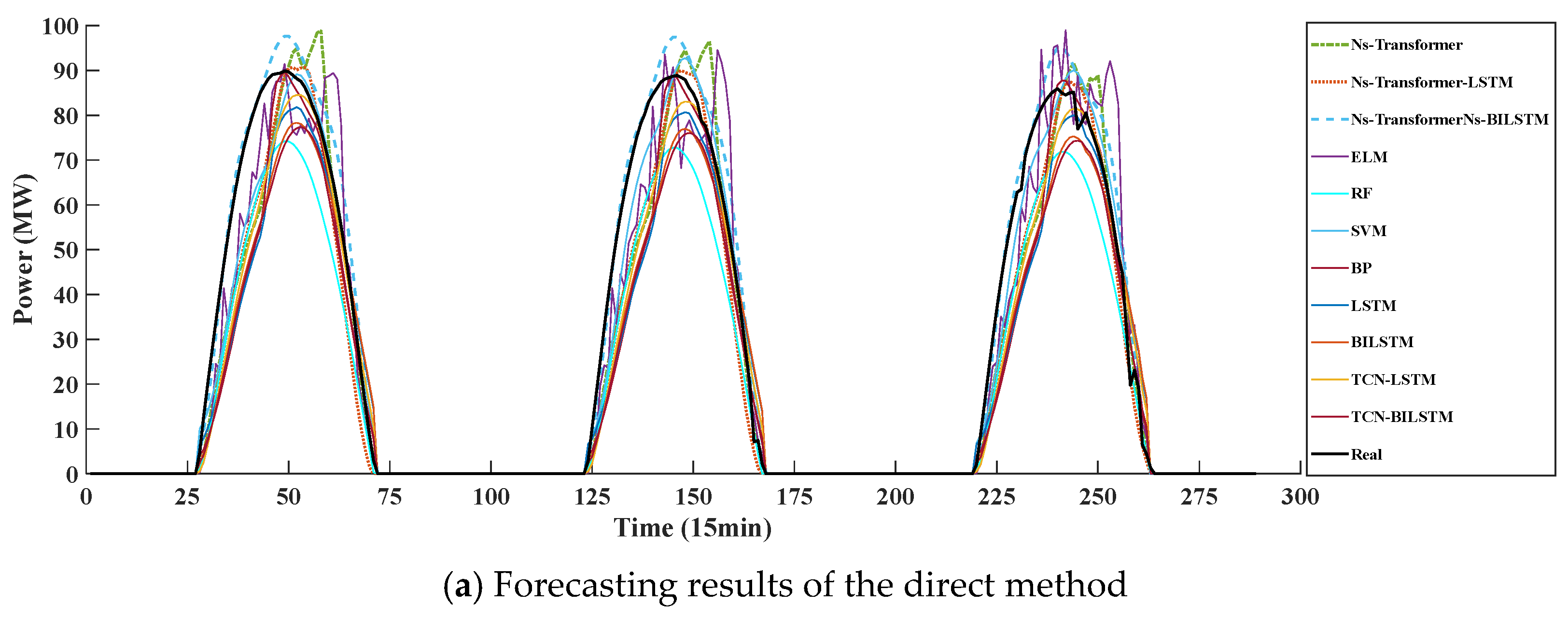
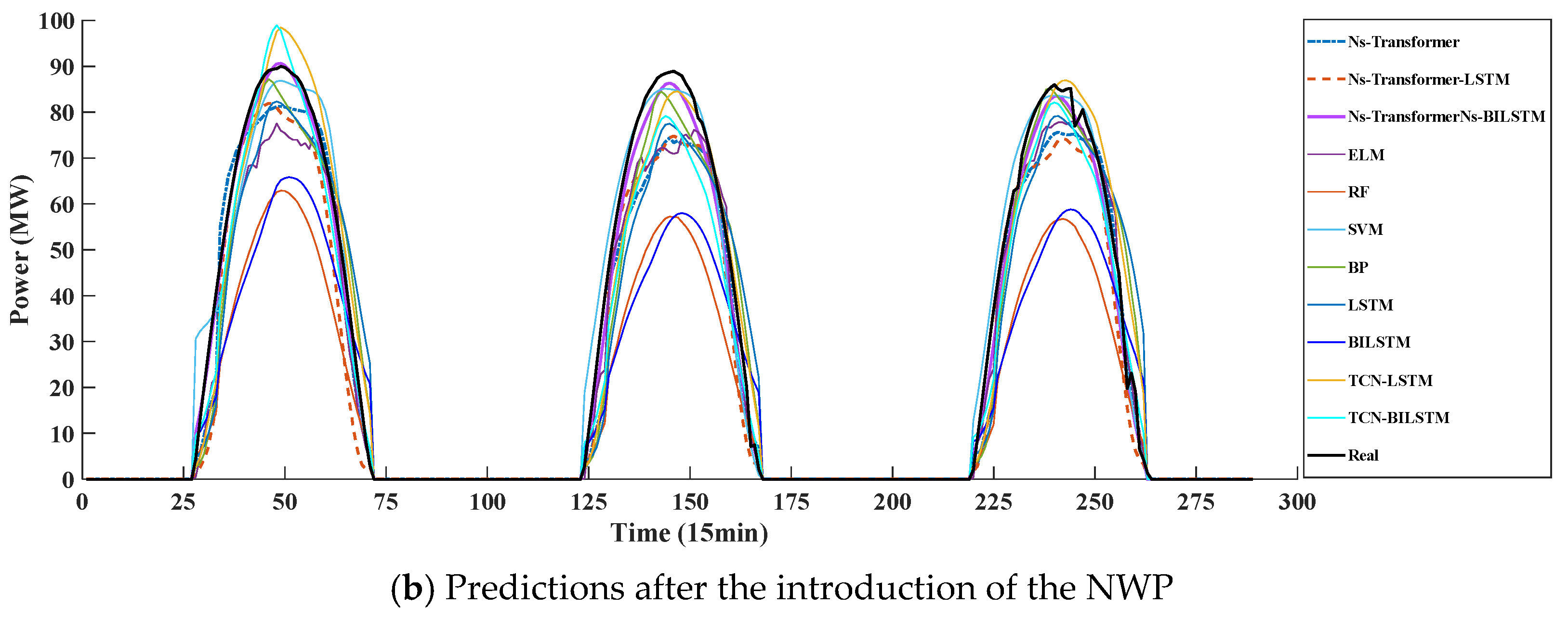
Ablation Experiment 1 employs conventional time-series forecasting to predict photovoltaic plant output using benchmark models. Input features comprise historical power data alongside key NWP variables for the target period: irradiance, temperature, cloud cover, and wind speed. Prediction error metrics (RMSE, MAE, R²) under NWP feature inclusion/exclusion regimes are detailed in

Table 4. Error evaluation indexes of different models using the direct prediction method.

Index	ELM	RF	SVM	BP	LSTM	BILSTM	TCN-LSTM	TCN-BILSTM	Transformer	Ns-Transformer
RMSE	0.1595	0.1613	0.1465	0.1431	0.1410	0.1422	0.1394	0.1392	0.1231	0.0876
MAE	0.0846	0.0724	0.0691	0.0707	0.0721	0.0718	0.0686	0.0729	0.0600	0.0325
R2	0.6766	0.6692	0.7272	0.7398	0.7473	0.7430	0.7530	0.7538	0.8373	0.9312

and

Table 5. Evaluation metrics of prediction error after introducing NWP in different models.

Index	ELM	RF	SVM	BP	LSTM	BILSTM	TCN-LSTM	TCN-BILSTM	Transformer	Ns-Transformer
RMSE	0.1429	0.1402	0.1376	0.1439	0.1586	0.1371	0.1280	0.1294	0.1252	0.0793
MAE	0.0683	0.0690	0.0626	0.0705	0.0827	0.0652	0.0599	0.0632	0.0594	0.0280
R2	0.7403	0.7502	0.7592	0.7367	0.6802	0.7610	0.7918	0.7870	0.8408	0.9404

, respectively. The direct method (historical power extrapolation) yields substantially elevated errors, with cross-model averages reaching RMSE = 0.1376, MAE = 0.0669, R² = 0.7599. Among these, RF exhibits maximal deviations (RMSE = 0.1613, MAE = 0.0724, R² = 0.6692). Hybrid architectures demonstrate superior performance, particularly the TCN-Ns-Transformer integration, which reduces RMSE/MAE by 2.48%/1.43% on average while elevating R² by 9.40% relative to peers. The standalone Ns-Transformer achieves optimal error suppression, registering 5.50% RMSE and 3.78% MAE reductions with 18.84% R² enhancement. NWP feature integration significantly refines forecasting precision, reducing average RMSE/MAE by 0.62%/0.45% and boosting R² by 2.13%. Crucially, our proposed composite model achieves minimal prediction error, outperforming alternatives by 5.74% RMSE, 3.79% MAE, and 17.51% R² margins. Figure 7 visualizes comparative prediction trajectories with/without NWP inputs. While our framework maintains robust accuracy across both conditions, transient fluctuation details remain challenging to capture during high-volatility episodes.

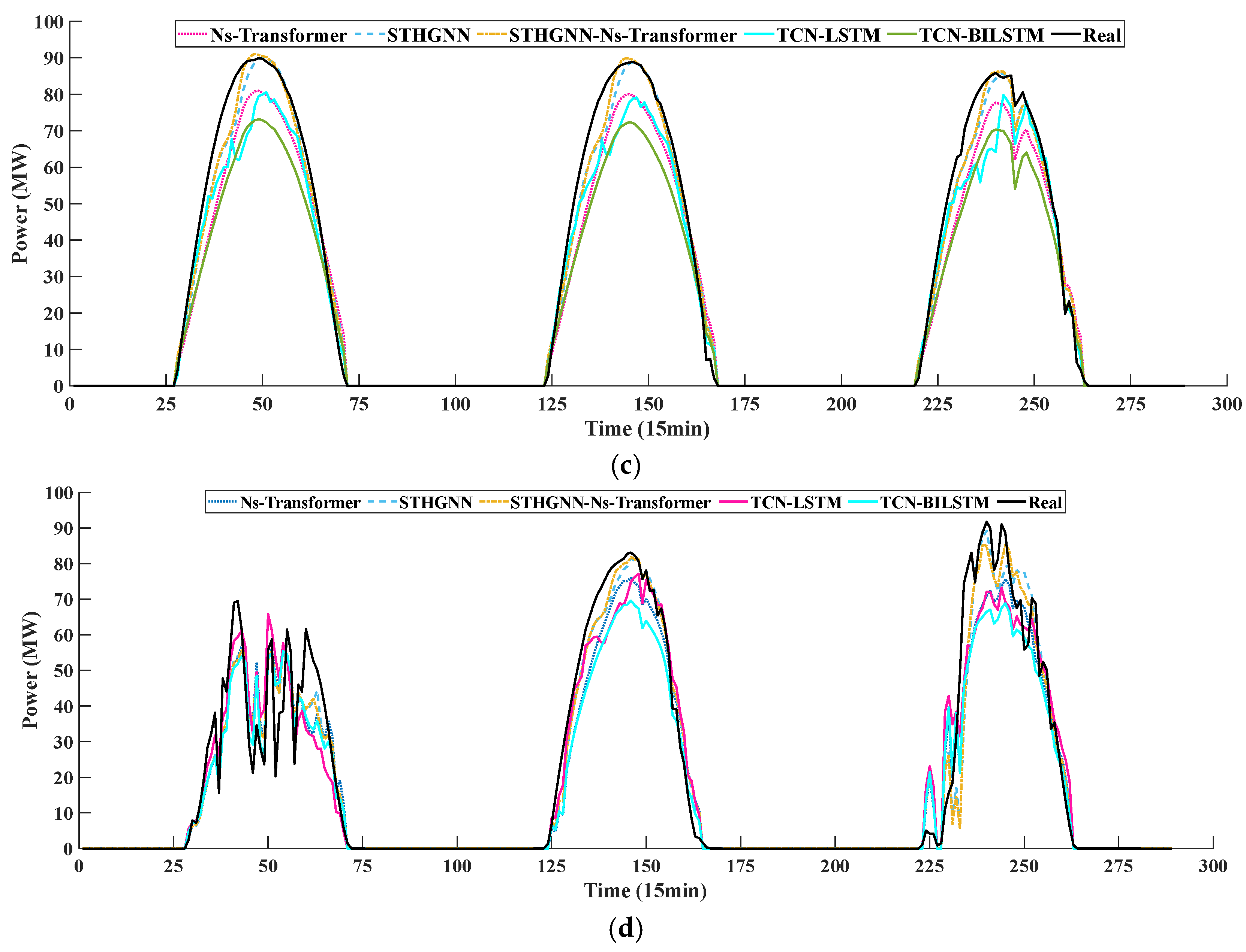
To address this, we conduct additional comparisons via Ablation Experiment 2. Here, the proposed prediction approach is evaluated against a baseline methodology involving full decomposition of meteorological and power data (termed Baseline Method 1). Benchmark models—including TCN-LSTM, TCN-BILSTM, Ns-Transformer, STHGNN, and the integrated STHGNN-Ns-Transformer—are employed for performance assessment. Prediction is executed through sequential component-wise forecasting followed by reconstruction.

Table 6. Evaluation indexes of prediction error for each model corresponding to the comparison of Method 1 and the proposed methodology.

Comparison Method	Index	TCN-LSTM	TCN-BILSTM	Ns-Transformer	STHGNN	STHGNN-Ns-Transformer
Comparison method 1	RMSE	0.1357	0.1122	0.1108	0.1001	0.0890
	MAE	0.0711	0.0583	0.0566	0.0488	0.0447
	R2	0.7660	0.8400	0.8440	0.8726	0.8993
Proposed method	RMSE	0.1221	0.1037	0.1004	0.0759	0.0689
	MAE	0.0418	0.0537	0.0471	0.0395	0.0332
	R2	0.8105	0.8633	0.8717	0.9268	0.9397

quantifies error metrics across both methodologies, revealing performance variations consistent with Ablation Experiment 1. Both Baseline Method 1 and our proposed framework demonstrate that TCN-LSTM/BILSTM ensembles exhibit inferior forecasting efficacy relative to Ns-Transformer variants and STHGNN architectures. Specifically, under Baseline Method 1, the Ns-Transformer configuration achieves mean reductions of 2.40% in RMSE and 1.47% in MAE alongside a 6.90% R² improvement compared to TCN hybrids. Conversely, our method yields greater enhancements: RMSE decreases by 3.11%, MAE by 0.78%, and R² increases by 7.58% versus TCN-based models. The RMSE and MAE of the proposed method are, on average, 1.53% and 1.28% lower, respectively, and R² is 3.80% higher than the TCN combinatorial model for all the models, compared to Method 1. STHGNN achieves a more significant prediction effect due to the use of multiple heterogeneous maps and the fusion of different information, with an average lower RMSE and MAE of 3.7%, 0.83% and a higher R² of 8.99% compared to the combined models of the TCN series when using the proposed prediction method. The proposed STHGNN-Ns-Transformer model, combined with the proposed method, has an average lower RMSE and MAE of 4.07%, 2.27%, and a higher R² of 9.53%, respectively, compared to the models in the Comparison Method 1. Figure 8 visually contrasts prediction curves generated by different methodologies and models. The direct decomposition approach exhibits weaker alignment with actual power trends compared to our proposed framework. Notably, our solution more accurately captures dynamic variations during fluctuating periods, yielding enhanced prediction precision.

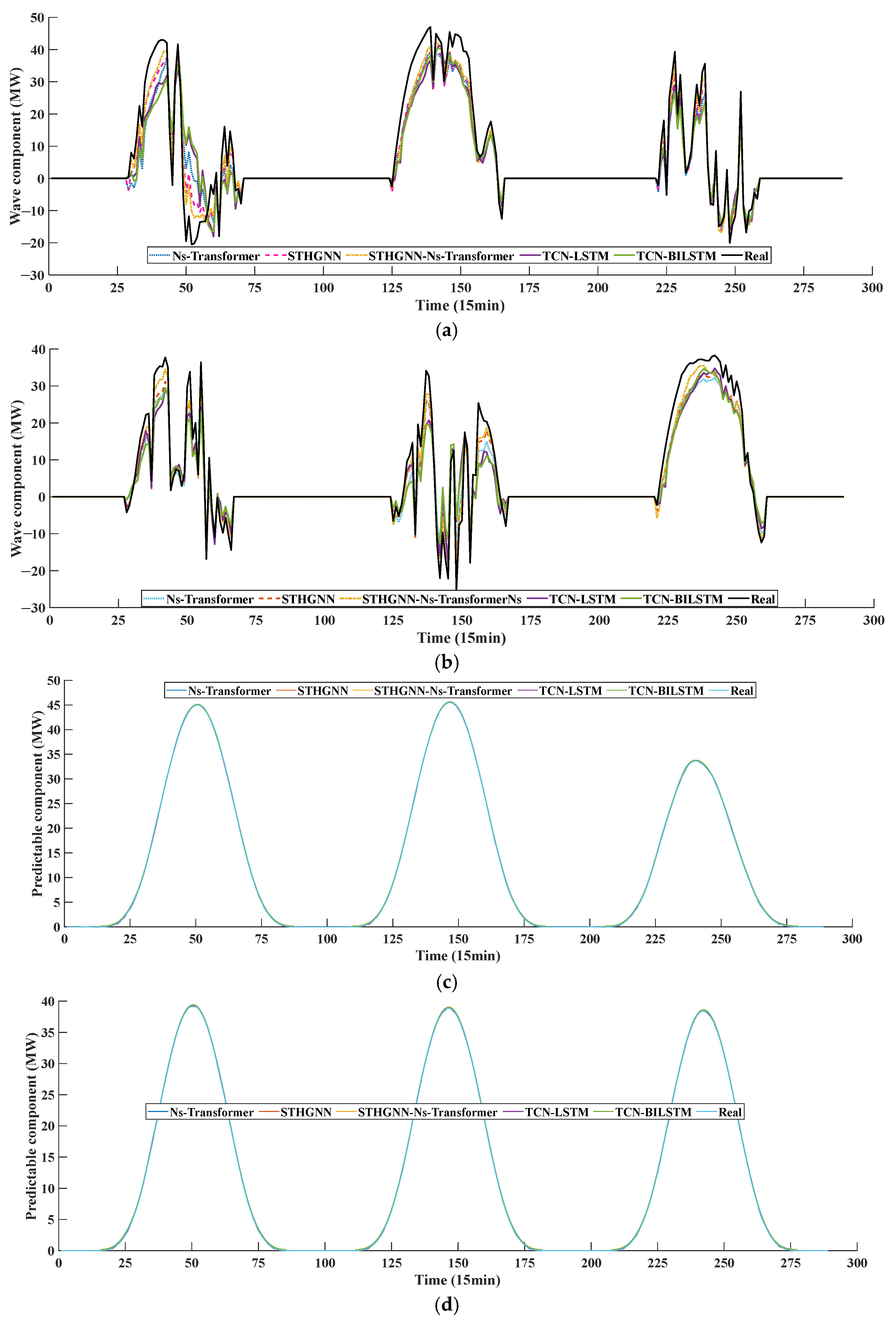
To evaluate our spatiotemporal heterogeneous graph framework against conventional multi-modeling techniques, Ablation Experiment 3 employs identical benchmark architectures (TCN-LSTM, TCN-BILSTM, Ns-Transformer, STHGNN, and STHGNN-Ns-Transformer). These assess two distinct approaches: multicomponent joint prediction (simultaneous forecasting of all component powers—implemented via multi-output schemes in TCN and the standalone Ns-Transformer) versus node information fusion (aggregating all node data into single-node representations before final output). Within this experiment, (1) our trend component extraction serves as primary data preprocessing, (2) multicomponent joint prediction constitutes the proposed methodology, and (3) node fusion modeling represents Comparative Method 2. Figure 9 illustrates our framework’s predictive performance for both trend and fluctuation sub-components within the decomposed fluctuating series. Crucially, CISSD-enhanced decomposition of fluctuation components into constituent elements substantially improves predictability, yielding measurable accuracy gains. Therefore, almost every model using the multi-node joint modelling architecture can obtain satisfactory prediction results, especially the STHGNN combined prediction model in this paper. As for the predictable components, almost every model obtains a high prediction accuracy, which is due to the fact that the predictability of the predictable components is fully considered in the reconstruction process, and the extracted predictable components have a high correlation with the predictable components of NWP irradiance.

Table 7. Evaluation indexes of prediction error for each model corresponding to the comparison of Method 1 and the proposed method.

Comparison Method	Index	TCN-LSTM	TCN-BILSTM	Ns-Transformer	STHGNN	STHGNN-Ns-Transformer
Comparison method 2	RMSE	0.1199	0.1198	0.0988	0.0872	0.0712
	MAE	0.0623	0.0621	0.0515	0.0427	0.0347
	R2	0.8172	0.8176	0.8759	0.9034	0.9355
Proposed method	RMSE	0.0572	0.0574	0.0551	0.0507	0.0414
	MAE	0.0292	0.0296	0.0284	0.0263	0.0217
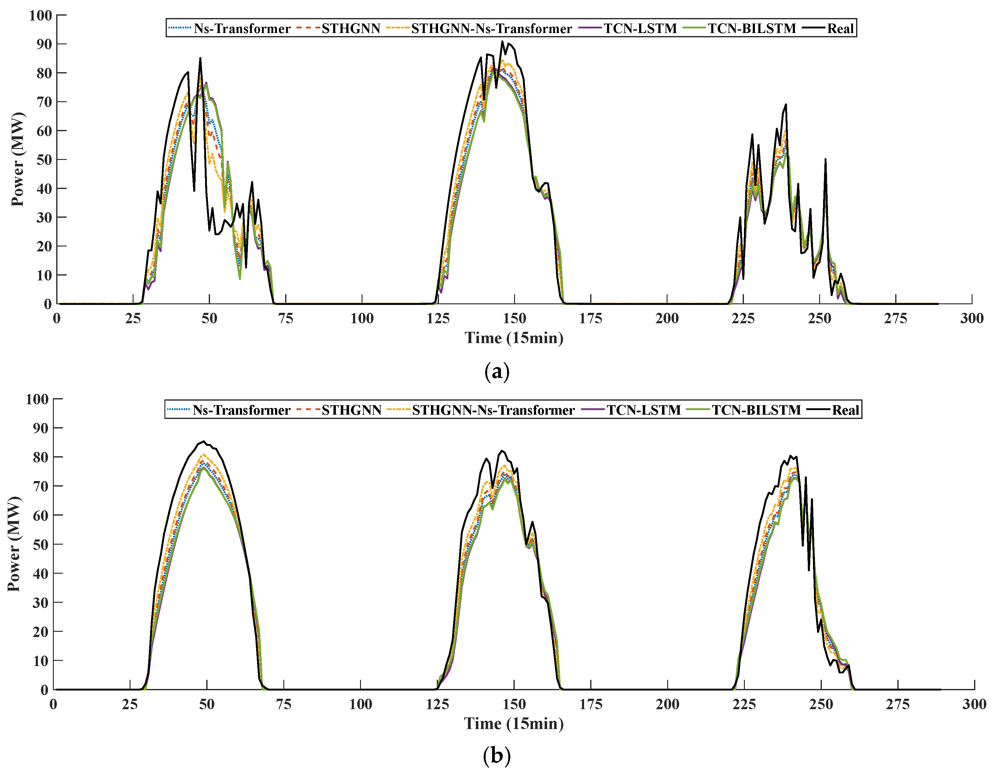
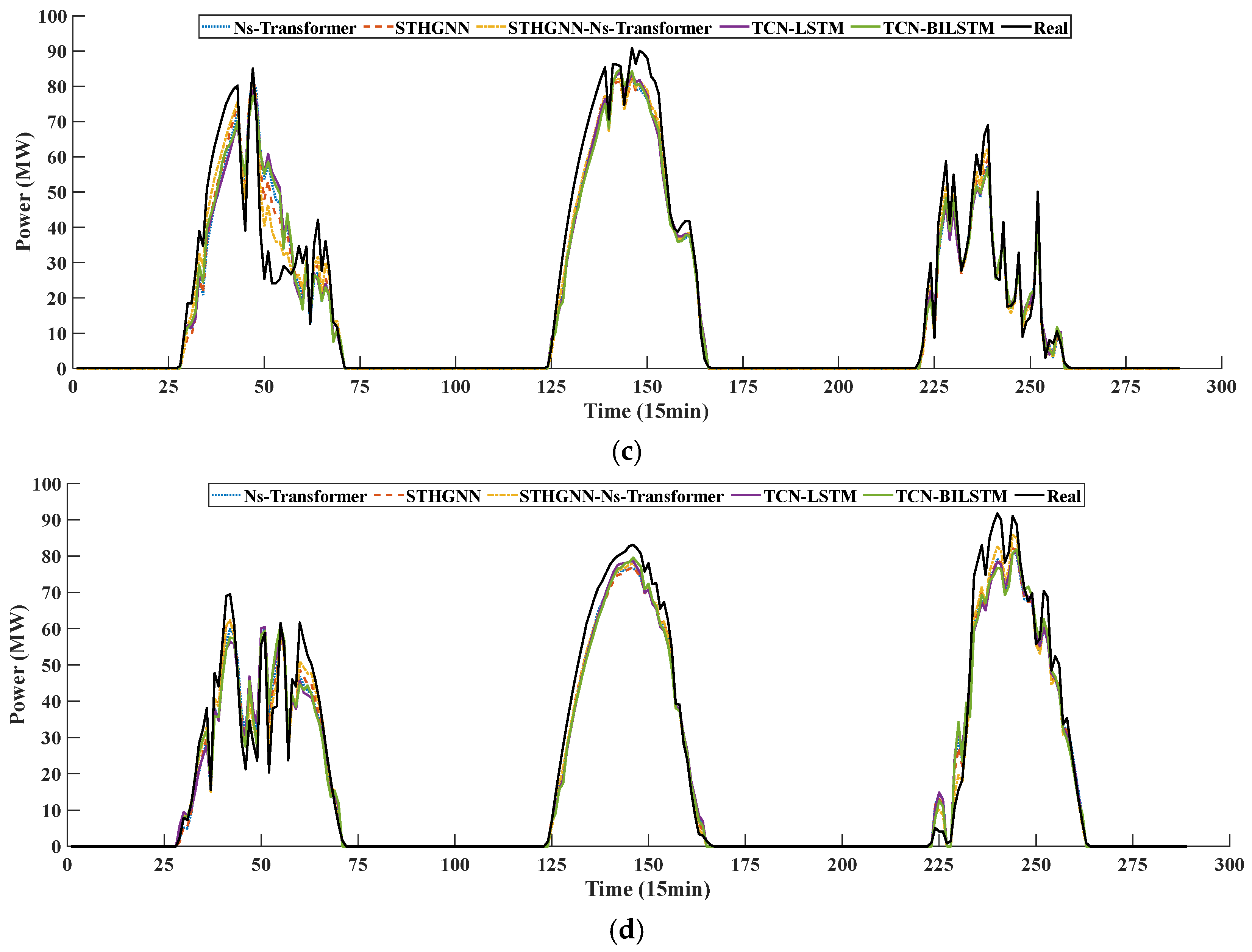
	R2	0.9584	0.9580	0.9614	0.9673	0.9782

quantitatively contrasts error metrics between Comparative Method 2 and our framework, demonstrating superior accuracy across both conventional forecasting and multi-node joint prediction paradigms when implementing our methodology. The spatiotemporal heterogeneous graph architecture substantially enhances power prediction precision, yielding average reductions of 4.70% in RMSE and 2.36% in MAE alongside a 9.47% R² improvement relative to Method 2. Furthermore, our STHGNN-Ns-Transformer configuration outperforms alternative models with additional decreases of 1.37% RMSE and 0.67% MAE, plus a 1.69% R² gain. Critically, when integrating predictable component extraction with multi-node joint prediction, this combined framework achieves mean reductions of 6.50% (RMSE) and 5.09% (MAE) alongside R² enhancements of 11.93% and 9.70% across evaluation scenarios. These performance differentials are visually substantiated in Figure 10, where our approach maintains higher accuracy in both fusion modeling and multi-node joint prediction contexts. Due to the completeness of input features and the capture of multi-node correlations by multiple heterogeneous graphs in multi-node joint prediction, the model learns more available information for improving the power prediction accuracy, and thus its prediction curve is closer to the real curve.

4. Analysis and Discussion

4.1. Comparison of Prediction Efficiency and Performance of Different Modelling Approaches

Our analysis of direct prediction, complete decomposition, and multi-node joint prediction models integrated with predictable component extraction validates the proposed methodology’s efficacy. Building upon these findings, we now critically examine the framework’s operational efficiency and computational burden. Notably, predictable component extraction coupled with multi-node joint prediction incurs the most substantial modeling costs. Consequently, this section conducts a systematic comparison between conventional modeling techniques and our approach, evaluating both temporal efficiency and predictive accuracy to holistically assess the proposed framework’s viability. Traditional methodologies primarily employ sequence decomposition via EMD, CEEMD, or similar techniques, subsequently combining high-performance prediction models for sequential component forecasting—a process whose computational demands center principally on decomposition operations, repeated model training, and optimization procedures, as shown in Figure 11.

Table 8. Training time cost of different prediction models in different comparison methods (Note: ’#’ indicates not applicable, bold indicates emphasis).

Comparison Method	TCN-LSTM	TCN-BILSTM	Ns-Transformer	STHGNN	STHGNN-Ns-Transformer
Comparison method 1 (s)	1206.1553	1302.4415	1506.1005	#	#
Comparison method 2 (s)	1201.4534	1291.4425	1521.4305	#	#
Proposed method (s)	#	#	#	310.2559	315.1491

compares the different modelling approaches and the training time cost of the models, in which the Comparison Methods 1 and 2 mainly use the traditional single-task learning mechanism, which needs to build a corresponding prediction model for each component, and thus the modelling cost is very high (the STHGNN modelling approach is not applicable to traditional single-node modelling, while traditional TCN-based and Ns-Transformer-based modelling approaches are not applicable to multi-node joint modelling). The proposed method, on the other hand, adopts a multi-node joint prediction modelling strategy, which trains the model once to achieve joint prediction for different components, and thus the time cost is much lower. The modelling cost corresponding to the proposed methods in this paper is, on average, 1128.8645 s lower than the rest of the methods, and the STHGNN-Ns-Transformer combined learning architecture using multi-node joint prediction can reduce the modelling time cost by 1214.0664 s on average compared with the combined model corresponding to the rest of the methods. The time consumption of the proposed method in this paper in the predictability component extraction session is higher than the traditional method by 47.4 s on average, but its decomposition performance is much higher than the rest of the models. As for the modelling session, this paper mainly uses a combined prediction method based on STHGNN combined with Ns-Transformer, which significantly reduces the modelling cost by more than 1100 s compared with the traditional single-node modelling strategy (The response time of different models in the prediction session is usually below 10 s). In terms of the total modelling cost, the method in this paper is significantly lower than the traditional method; the training model can be obtained, and high-performance prediction can be achieved in a short time. Meanwhile, this paper further analyzes the distribution results of the hour-by-hour prediction errors of the above three modelling methods corresponding to different models, as shown in Figure 12. Our approach demonstrates significantly reduced median hourly error relative to Comparative Methods 1 and 2. Furthermore, enhanced error concentration within lower intervals substantiates its capacity to sustain superior prediction accuracy across short timeframes despite requiring reduced computational expenditure.

4.2. Generalisability Analysis of the Proposed Method

Examining the prediction performance of different prediction schemes in differentiated PV stations is necessary because the proposed method that exhibits prediction performance bias or even significant deterioration in accuracy in unknown or significantly differentiated regions may lead to limited generalization of the method and is not suitable for generalized applications. In this regard, we introduce more PV stations from different locations, including: two PV stations in two geographic locations in China, such as Jilin and Guizhou provinces, which contain the same types of forecasting and measured data as the Gansu PV station, with a temporal resolution of 15 min and a spatial resolution of 3 km × 3 km, and we apply the proposed method to the different PV stations for power prediction.

Table 9. Power prediction error assessment metrics in new PV stations using different methodologies.

Station	Index	TCN-LSTM	TCN-BILSTM	Ns-Transformer	STHGNN	STHGNN-Ns-Transformer
Jilin-station	RMSE	0.0561	0.0554	0.0502	0.0487	0.0404
	MAE	0.0294	0.0246	0.0202	0.0198	0.0187
	R2	0.9514	0.968	0.9884	0.9893	0.9982
Guizhou-station	RMSE	0.0602	0.0634	0.0553	0.0527	0.0417
	MAE	0.0332	0.0346	0.0287	0.0274	0.0225
	R2	0.9184	0.908	0.9654	0.9603	0.9682

shows the power prediction error assessment indexes corresponding to different modeling approaches for the new PV stations, where different modeling approaches correspond to different error assessment indexes, and the STHGNN based on the multi-node joint modeling achieves significant prediction accuracy enhancement compared to the traditional model, especially the combined prediction model combining Ns-Transformer. In the stations in Jilin, the STHGNN-based modeling approach achieves an average of 0.52% and 0.49% lower RMSE and MAE than the traditional model, respectively, while the R² is improved by 2.00% on average, and the combined prediction model based on the STHGNN-Ns-Transformer achieves an average of 1.35% and 0.60% lower RMSE and MAE than the traditional approach, respectively, while the R² is improved by 2.89% on average. In the stations in Guizhou, the STHGNN-based modeling approach has an average lower predictive RMSE and MAE than the traditional model by 0.69% and 0.48%, respectively, while the R² is improved by 2.97% on average, and the combined predictive model based on STHGNN-Ns-Transformer has an average lower predictive RMSE and MAE than the traditional approach by 1.79% and 0.97%, while R² is improved by 3.76% on average. In almost every station, the combined prediction model of STHGNN combined with Ns-Transformer proposed in this paper significantly improves the power predictability and achieves high prediction accuracy through the methods of irradiation correction and predictable component extraction.

5. Conclusions

This paper presents a novel ultra-short-term photovoltaic power forecasting framework integrating predictable component extraction/reconstruction with optimized multi-node spatiotemporal heterogeneous graph architecture, substantially enhancing fluctuation component prediction. Key findings reveal the following:

(1)

Hybrid models exhibit superior performance, with TCN-Ns-Transformer configurations reducing RMSE and MAE by 2.48% and 1.43%, respectively, while increasing R² by 9.40% versus alternatives. Our STHGNN-Ns-Transformer achieves the lowest prediction error, demonstrating 5.50% RMSE reduction, 3.78% MAE improvement, and 18.84% R² enhancement over benchmark models. This integrated architecture further outperforms Comparative Method 1 by 4.07% RMSE, 2.27% MAE, and 9.53% R² gains.

(2)

The spatiotemporal heterogeneous framework elevates forecasting precision, reducing RMSE by 4.70% and MAE by 2.36% against Comparative Method 2 while boosting R² by 9.47%. Specifically, STHGNN-Ns-Transformer decreases RMSE by 1.37% and MAE by 0.67% compared to other architectures, with 1.69% R² improvement. When incorporating predictable component extraction into multi-node joint prediction, the system achieves combined reductions of 6.50%/5.09% (RMSE) and 2.50%/2.46% (MAE), plus R² enhancements of 11.93%/9.70%.

While this framework significantly improves standard ultra-short-term forecasting, extreme scenario accuracy remains challenging. Future work will investigate meteorological correction and predictive feature mining under such conditions to enhance prediction robustness.

References

1. Fu, X. Statistical machine learning model for capacitor planning considering uncertainties in photovoltaic power. Prot. Control Mod. Power Syst. 2022, 7, 1–13. [Google Scholar] [CrossRef]
2. Zhi, Y.; Sun, T.; Yang, X. A physical model with meteorological forecasting for hourly rooftop photovoltaic power prediction. J. Build. Eng. 2023, 75, 106997. [Google Scholar] [CrossRef]
3. Yang, M.; Jiang, Y.; Zhang, W.; Li, Y.; Su, X. Short-term Interval Prediction Strategy of Photovoltaic Power Based on Meteorological Reconstruction with Spatiotemporal Correlation and Multi-factor Interval Constraints. Renew. Energy 2024, 237, 121834. [Google Scholar] [CrossRef]
4. Mayer, M.J.; Yang, D. Pairing ensemble numerical weather prediction with ensemble physical model chain for probabilistic photovoltaic power forecasting. Renew. Sustain. Energy Rev. 2023, 175, 113171. [Google Scholar] [CrossRef]
5. Jackson, N.D.; Gunda, T. Evaluation of extreme weather impacts on utility-scale photovoltaic plant performance in the United States. Appl. Energy 2021, 302, 117508. [Google Scholar] [CrossRef]
6. Markovics, D.; Mayer, M.J. Comparison of machine learning methods for photovoltaic power forecasting based on numerical weather prediction. Renew. Sustain. Energy Rev. 2022, 161, 112364. [Google Scholar] [CrossRef]
7. Jamil, I.; Lucheng, H.; Iqbal, S.; Aurangzaib, M.; Jamil, R.; Kotb, H.; Alkuhayli, A.; AboRas, K.M. Predictive evaluation of solar energy variables for a large-scale solar power plant based on triple deep learning forecast models. Alex. Eng. J. 2023, 76, 51–73. [Google Scholar] [CrossRef]
8. Libra, M.; Kozelka, M.; Šafránková, J.; Belza, R.; Poulek, V.; Beránek, V.; Sedláček, J.; Zholobov, M.; Šubrt, T.; Severová, L. Agrivoltaics: Dual usage of agricultural land for sustainable development. Int. Int. Agrophysics 2024, 38, 121–126. [Google Scholar] [CrossRef]
9. Liu, W.; Liu, Q.; Li, Y. Ultra-short-term photovoltaic power prediction based on modal reconstruction and BiLSTM-CNN-Attention model. Earth Sci. Inform. 2024, 17, 2711–2725. [Google Scholar] [CrossRef]
10. Khelifi, R.; Guermoui, M.; Rabehi, A.; Taallah, A.; Zoukel, A.; Ghoneim, S.S.M.; Bajaj, M.; AboRas, K.M.; Zaitsev, I.; Falabretti, D. Short-Term PV Power Forecasting Using a Hybrid TVF-EMD-ELM Strategy. Int. Trans. Electr. Energy Syst. 2023, 2023, 6413716. [Google Scholar] [CrossRef]
11. Yang, M.; Guo, Y.; Fan, F. Ultra-short-term prediction of wind farm cluster power based on embedded graph structure learning with spatiotemporal information gain. IEEE Trans. Sustain. Energy 2024, 16, 308–322. [Google Scholar] [CrossRef]
12. Simeunovic, J.; Schubnel, B.; Alet, P.-J.; Carrillo, R.E. Spatio-temporal graph neural networks for multi-site PV power forecasting. IEEE Trans. Sustain. Energy 2021, 13, 1210–1220. [Google Scholar] [CrossRef]
13. Zhang, M.; Zhen, Z.; Liu, N.; Zhao, H.; Sun, Y.; Feng, C.; Wang, F. Optimal graph structure based short-term solar PV power forecasting method considering surrounding spatio-temporal correlations. IEEE Trans. Ind. Appl. 2022, 59, 345–357. [Google Scholar] [CrossRef]
14. Li, Z.; Ye, L.; Song, X.; Luo, Y.; Pei, M.; Wang, K.; Yu, Y.; Tang, Y. Heterogeneous spatiotemporal graph convolution network for multi-modal wind-PV power collaborative prediction. IEEE Trans. Power Syst. 2023, 39, 5591–5608. [Google Scholar] [CrossRef]
15. Yang, M.; Guo, Y.; Huang, T.; Fan, F.; Ma, C.; Fang, G. Wind farm cluster power prediction based on graph deviation attention network with learnable graph structure and dynamic error correction during load peak and valley period. Energy 2024, 312, 133645. [Google Scholar] [CrossRef]
16. Semero, Y.K.; Zhang, J.; Zheng, D. PV power forecasting using an integrated GA-PSO-ANFIS approach and Gaussian process regression based feature selection strategy. CSEE J. Power Energy Syst. 2018, 4, 210–218. [Google Scholar] [CrossRef]
17. Liu, R.; Wei, J.; Sun, G.; Muyeen, S.; Lin, S.; Li, F. A short-term probabilistic photovoltaic power prediction method based on feature selection and improved LSTM neural network. Electr. Power Syst. Res. 2022, 210, 108069. [Google Scholar] [CrossRef]
18. Niu, D.; Wang, K.; Sun, L.; Wu, J.; Xu, X. Short-term photovoltaic power generation forecasting based on random forest feature selection and CEEMD: A case study. Appl. Soft Comput. 2020, 93, 106389. [Google Scholar] [CrossRef]
19. Zhou, H.; Zheng, P.; Dong, J.; Liu, J.; Nakanishi, Y. Interpretable feature selection and deep learning for short-term probabilistic PV power forecasting in buildings using local monitoring data. Appl. Energy 2024, 376, 124271. [Google Scholar] [CrossRef]
20. Chen, H.; Chang, X. Photovoltaic power prediction of LSTM model based on Pearson feature selection. Energy Rep. 2021, 7, 1047–1054. [Google Scholar] [CrossRef]
21. Huang, N.; Li, R.; Lin, L.; Yu, Z.; Cai, G. Low redundancy feature selection of short term solar irradiance prediction using conditional mutual information and Gauss process regressio. Sustainability 2018, 10, 2889. [Google Scholar] [CrossRef]
22. Acikgoz, H. A novel approach based on integration of convolutional neural networks and deep feature selection for short-term solar radiation forecastin. Appl. Energy 2022, 305, 117912. [Google Scholar] [CrossRef]
23. Zhang, C.; Peng, T.; Nazir, M.S. A novel integrated photovoltaic power forecasting model based on variational mode decomposition and CNN-BiGRU considering meteorological variables. Electr. Power Syst. Res. 2022, 213, 108796. [Google Scholar] [CrossRef]
24. Zhang, M.; Han, Y.; Wang, C.; Yang, P.; Wang, C.; Zalhaf, A.S. Ultra-short-term photovoltaic power prediction based on similar day clustering and temporal convolutional network with bidirectional long short-term memory model: A case study using DKASC data. Appl. Energy 2024, 375, 124085. [Google Scholar] [CrossRef]
25. Zha, W.; Liu, J.; Li, Y.; Liang, Y. Ultra-short-term power forecast method for the wind farm based on feature selection and temporal convolution network. ISA Trans. 2022, 129, 405–414. [Google Scholar] [CrossRef] [PubMed]
26. Xiang, X.; Li, X.; Zhang, Y.; Hu, J. A short-term forecasting method for photovoltaic power generation based on the TCN-ECANet-GRU hybrid model. Sci. Rep. 2024, 14, 6744. [Google Scholar] [CrossRef] [PubMed]
27. Chen, H.; Zhu, M.; Hu, X.; Wang, J.; Sun, Y.; Yang, J.; Li, B.; Meng, X.; Prusty, B.R. Multifeature Short-Term Power Load Forecasting Based on GCN-LSTM. Int. Trans. Electr. Energy Syst. 2023, 2023, 8846554. [Google Scholar] [CrossRef]
28. Yang, L.; Miao, Z.; Li, T.; Tan, S.; Wang, B.; Li, D.; Liu, Y.; Wei, H.; Li, J.; Li, J.; et al. LSTM-GCN based multidimensional parameter relationship analysis and prediction framework for system level experimental bench. Ann. Nucl. Energy 2025, 210, 110890. [Google Scholar] [CrossRef]
29. Abedinia, O.; Lotfi, M.; Bagheri, M.; Sobhani, B.; Shafie-Khah, M.; Catalao, J.P.S. Improved EMD-based complex prediction model for wind power forecasting. IEEE Trans. Sustain. Energy 2020, 11, 2790–2802. [Google Scholar] [CrossRef]
30. Wang, H.; Sun, J.; Wang, W. Photovoltaic power forecasting based on EEMD and a variable-weight combination forecasting model. Sustainability 2018, 10, 2627. [Google Scholar] [CrossRef]
31. Bommidi, B.S.; Teeparthi, K.; Kosana, V. Hybrid wind speed forecasting using ICEEMDAN and transformer model with novel loss functio. Energy 2023, 265, 126383. [Google Scholar] [CrossRef]
32. Gun, A.R.; Dokur, E.; Yuzgec, U.; Kurban, M. Short-Term Solar Power Forecasting Based on CEEMDAN and Kernel Extreme Learning Machine. Elektron. Elektrotechnika 2023, 29, 28–34. [Google Scholar] [CrossRef]
33. Cui, S.; Lyu, S.; Ma, Y.; Wang, K. Improved informer PV power short-term prediction model based on weather typing and AHA-VMD-MPE. Energy 2024, 307, 132766. [Google Scholar] [CrossRef]
34. Jamei, M.; Ali, M.; Karbasi, M.; Karimi, B.; Jahannemaei, N.; Farooque, A.A.; Yaseen, Z.M. Monthly sodium adsorption ratio forecasting in rivers using a dual interpretable glass-box complementary intelligent system: Hybridization of ensemble TVF-EMD-VMD, Boruta-SHAP, and eXplainable GPR. Expert Syst. Appl. 2024, 237, 121512. [Google Scholar] [CrossRef]
35. Bai, R.; Shi, Y.; Yue, M.; Du, X. Hybrid model based on K-means++ algorithm, optimal similar day approach, and long short-term memory neural network for short-term photovoltaic power prediction. Glob. Energy Interconnect. 2023, 6, 184–196. [Google Scholar] [CrossRef]
36. Zhou, Y.; Zhou, N.; Gong, L.; Jiang, M. Prediction of photovoltaic power output based on similar day analysis, genetic algorithm and extreme learning machine. Energy 2020, 204, 117894. [Google Scholar] [CrossRef]
37. Li, Y.; Huang, W.; Lou, K.; Zhang, X.; Wan, Q. Short-term PV power prediction based on meteorological similarity days and SSA-BiLSTM. Syst. Soft Comput. 2024, 6, 200084. [Google Scholar] [CrossRef]
38. Gao, M.; Li, J.; Hong, F.; Long, D. Day-ahead power forecasting in a large-scale photovoltaic plant based on weather classification using LSTM. Energy 2019, 187, 115838. [Google Scholar] [CrossRef]
39. Zhou, Y.; Wang, J.; Li, Z.; Lu, H. Short-term photovoltaic power forecasting based on signal decomposition and machine learning optimizatio. Energy Convers. Manag. 2022, 267, 115944. [Google Scholar] [CrossRef]
40. Zhang, C.; Zhang, F.; Gou, F.; Cao, W. Study on short-term electricity load forecasting based on the modified simplex approach sparrow search algorithm mixed with a bidirectional long-and short-term memory network. Processes 2024, 12, 1796. [Google Scholar] [CrossRef]
41. Ge, L.; Xian, Y.; Yan, J.; Wang, B.; Wang, Z. A hybrid model for short-term PV output forecasting based on PCA-GWO-GRNN. J. Mod. Power Syst. Clean Energy 2020, 8, 1268–1275. [Google Scholar] [CrossRef]
42. He, Q.; Li, S. Gray relational analysis and SBOA-BP for predicting settlement intervals of high-speed railway subgrade. Railw. Sci. 2025, 4, 199–212. [Google Scholar] [CrossRef]
43. Jiang, J.; Hu, S.; Xu, L.; Wang, T. Short-term PV power prediction based on VMD-CNN-IPSO-LSSVM hybrid model. Int. J. Low-Carbon Technol. 2024, 19, 1160–1167. [Google Scholar] [CrossRef]
44. Zhang, Y.; Han, J.; Pan, G.; Xu, Y.; Wang, F. A multi-stage predicting methodology based on data decomposition and error correction for ultra-short-term wind energy prediction. J. Clean. Prod. 2021, 292, 125981. [Google Scholar] [CrossRef]
45. Geng, D.; Wang, B.; Gao, Q. A hybrid photovoltaic/wind power prediction model based on Time2Vec, WDCNN and BiLSTM. Energy Convers. Manag. 2023, 291, 117342. [Google Scholar] [CrossRef]
46. Niu, D.; Yu, M.; Sun, L.; Gao, T.; Wang, K. Short-term multi-energy load forecasting for integrated energy systems based on CNN-BiGRU optimized by attention mechanis. Appl. Energy 2022, 313, 118801. [Google Scholar] [CrossRef]
47. Yin, L.; Sun, Y. BiLSTM-InceptionV3-Transformer-fully-connected model for short-term wind power forecasting. Energy Convers. Manag. 2024, 321, 119094. [Google Scholar] [CrossRef]
48. Wang, S.; Shi, J.; Yang, W.; Yin, Q. High and low frequency wind power prediction based on Transformer and BiGRU-Attentio. Energy 2024, 288, 129753. [Google Scholar] [CrossRef]
49. Zhang, R.; Li, G.; Bu, S.; Kuang, G.; He, W.; Zhu, Y.; Aziz, S. A hybrid deep learning model with error correction for photovoltaic power forecasting. Front. Energy Res. 2022, 10, 948308. [Google Scholar] [CrossRef]
50. Li, G.; Wei, X.; Yang, H. Decomposition integration and error correction method for photovoltaic power forecasting. Measurement 2023, 208, 112462. [Google Scholar] [CrossRef]
51. Yin, W.; Han, Y.; Zhou, H.; Ma, M.; Li, L.; Zhu, H. A novel non-iterative correction method for short-term photovoltaic power forecasting. Renew. Energy 2020, 159, 23–32. [Google Scholar] [CrossRef]
52. Chen, J.; Peng, T.; Qian, S.; Ge, Y.; Wang, Z.; Nazir, M.S.; Zhang, C. An error-corrected deep Autoformer model via Bayesian optimization algorithm and secondary decomposition for photovoltaic power prediction. Appl. Energy 2025, 377, 124738. [Google Scholar] [CrossRef]
53. Bógalo, J.; Poncela, P.; Senra, E. Circulant singular spectrum analysis: A new automated procedure for signal extraction. Signal Process. 2021, 179, 107824. [Google Scholar] [CrossRef]
54. Luan, T.M.; Khatir, S.; Tran, M.T.; De Baets, B.; Cuong-Le, T. Exponential-trigonometric optimization algorithm for solving complicated engineering problems. Comput. Methods Appl. Mech. Eng. 2024, 432, 117411. [Google Scholar] [CrossRef]
55. Yang, M.; Guo, Y.; Fan, F.; Huang, T. Two-stage correction prediction of wind power based on numerical weather prediction wind speed superposition correction and improved clustering. Energy 2024, 302, 131797. [Google Scholar] [CrossRef]
56. Yang, M.; Jiang, Y.; Guo, Y.; Su, X.; Li, Y.; Huang, T. Ultra-short-term Prediction of Photovoltaic Cluster Power Based on Spatiotemporal Convergence Effect and Spatiotemporal Dynamic Graph Attention Network. Renew. Energy 2025, 255, 123843. [Google Scholar] [CrossRef]
57. Yang, M.; Guo, Y.; Huang, Y. Wind power ultra-short-term prediction method based on NWP wind speed correction and double clustering division of transitional weather process. Energy 2023, 282, 128947. [Google Scholar] [CrossRef]
58. Liu, Y.; Wu, H.; Wang, J.; Long, M. Non-stationary transformers: Exploring the stationarity in time series forecasting. Adv. Neural Inf. Process. Syst. 2022, 35, 9881–9893. [Google Scholar]
59. Yang, M.; Guo, Y.; Huang, T.; Zhang, W. Power prediction considering NWP wind speed error tolerability: A strategy to improve the accuracy of short-term wind power prediction under wind speed offset scenarios. Appl. Energy 2025, 377, 124720. [Google Scholar] [CrossRef]
60. Yang, M.; Guo, Y.; Wang, B.; Wang, Z.; Chai, R. A day-ahead wind speed correction method: Enhancing wind speed forecasting accuracy using a strategy combining dynamic feature weighting with multi-source information and dynamic matching with improved similarity function. Expert Syst. Appl. 2025, 263, 125724. [Google Scholar] [CrossRef]
Figure 1. Schematic diagram of the combined architecture based on STHGNN combined with Ns-Transformer.
Energies 18 04192 g001
Figure 2. Overall research technology framework.
Energies 18 04192 g002
Figure 3. Optimization fitness curves corresponding to different optimization algorithms.
Energies 18 04192 g003
Figure 4. Decomposition results of CISSD-based forecast irradiance series.
Energies 18 04192 g004
Figure 5. Extraction results of irradiance/power components.
Energies 18 04192 g005aEnergies 18 04192 g005b
Figure 6. (a) Decomposition results for the historical irradiance fluctuation component; (b) Decomposition results for historical power fluctuation components. Extraction results of irradiance/power fluctuation components.
Energies 18 04192 g006
Figure 7. Prediction curves of different models before and after the introduction of NWP.
Energies 18 04192 g007aEnergies 18 04192 g007b
Figure 8. (a) Comparison of Method 1 prediction curves—time period I; (b) Comparison of prediction curves for Method 1—time period II; (c) Prediction curves of the proposed methodology—time period I; (d) Prediction curves of the proposed methodology—time period II. Prediction curves of different prediction models corresponding to different prediction methods.
Energies 18 04192 g008aEnergies 18 04192 g008b
Figure 9. (a) Prediction results of the proposed method for the volatility component-I; (b) Prediction results of the proposed method for the fluctuation component-II; (c) Prediction results of the proposed method for the trend component-I; (d) Prediction results of the proposed method for the trend component-II. Prediction curves of the volatile and predictable components for different models using the method of this paper.
Energies 18 04192 g009
Figure 10. (a) Prediction results of the proposed method in node fusion modelling; (b) Prediction results of the proposed method in node fusion modelling-II; (c) Prediction results of the proposed method in multi-node joint prediction-I; (d) Prediction results of the proposed method in multi-node joint prediction-II. Prediction curves of different models in different prediction methods.
Energies 18 04192 g010aEnergies 18 04192 g010b
Figure 11. Decomposition time cost corresponding to different decomposition methods.
Energies 18 04192 g011
Figure 12. Hourly error distribution for different methods and models.
Energies 18 04192 g012