Comparative of IEC 60891 and Other Procedures for Temperature and Irradiance Corrections to Measured I–V Characteristics of Photovoltaic Devices

Abstract

The photovoltaic literature contains a wide range of methods for translating the I–V curves of a solar device to other conditions of irradiance and cell temperature, different from those under which the measurements were performed. Some of these translation methods are included as part of the International Standard IEC 60891. In this paper, these techniques are classified, reviewed, and implemented to perform a deep comparative analysis between them and to discuss their suitability for converting the I–V curves of photovoltaic modules under different scenarios of irradiance and temperature. From the analysis conducted, it can be seen that the interpolation method proposed in IEC 60891 achieves accurate results when it is applied to correct small and medium irradiance and temperature gaps. If no interpolation is possible and for large irradiance corrections, other procedures described in IEC 60891 can be applied. However, certain explicit methods based on the single-diode model or on the double-diode model can overcome the most well-known approaches proposed by the standard.

1. Introduction

Translating the current–voltage (I–V) curves of photovoltaic (PV) modules to different conditions of incident irradiance G and cell temperature T in an accurate and reliable way is essential for two reasons. First, it is necessary to enable meaningful comparisons between measurements. For example, to compare the performance of different solar cells or to assess the degradation in time of a PV module. For these comparisons, a reference set of test conditions, such as the Standard Test Conditions (STC) defined in IEC 60904-3 [1] are widely used. This conversion is especially needed when the measurement of the I–V curve is performed outdoors, where it is not possible to make the irradiance and temperature conditions equal to the STCs.

A second situation in which translating I–V curves is necessary is in the estimation of the energy yield of PV systems. This task requires the estimation of PV module efficiency under different operating conditions. These conditions typically include a wide range of irradiance and temperature values, for which the I–V curves are not available and need to be calculated from the curves under known conditions. A possible solution to this problem consists in applying to each measured I–V curve a corrective mathematical procedure that estimates how this curve would be if it were measured under a different set of irradiance and temperature conditions. Sandstrom [2] published, in 1967, the best known translation method, which has been widely used since then, and which was years later included in the International Standard IEC 60891 [3] as procedure 1.

Anderson [4] published a new set of equations for solving some incorrectness in [2], and this new approach was adopted in ASTM E 1036–02 [5]. However, the latter versions of the same standard, see ASTM E 1036–15(2019) [6], have moved to recommending a bilinear interpolation method proposed by Marion et al. [7], that requires four measured I–V curves as input. In the Standard IEC 60891 [3], there is a procedure (procedure 3) that is also based on an interpolation method, using three measured curves. In fact, there are many other approaches to performing a I–V curve correction. Selection of the best-known methods and a comparative analysis between them are performed.

The remainder of this article has the following structure: Section 1.1 includes a new classification of the correction procedures, whereas Section 1.2 reviews the most interesting methods. In Section 2, the PV modules under study are presented and the experiments are described. Section 3 analyses the obtained results for each studied approach. Finally, Section 4 presents the conclusions.

1.1. Classification of the Methods

Many methods have been published in the literature aimed at achieving this objective, i.e., correcting the I–V curve of a solar device for different conditions of irradiance and temperature than those under which it was measured. Herrmann and Wiesner [8] proposed a basic classification of these methods into algebraic methods (based on a shift of each discrete point) and numerical methods, which requires a curve fitting optimization over all the points of the curve to determine the model parameters: the photo-generated current $I_{ph}$, the dark-saturation current $I_s$, the diode ideality factor m, the series resistance $R_s$, and parallel resistance $R_{sh}$. The latter methods assume an underlying equivalent circuit, which could be the single-diode model (SDM) or the double-diode model (DDM).

In this work, several additional categories of methods are considered: analytical methods are those in which the curve fitting is replaced by a system of equations to be solved using the main electrical parameters as inputs (instead of all the points of the curve); explicit methods, based on the previous approach but with a very low computational burden, because they propose a sequence of simple explicit expressions to obtain the intrinsic parameters; iterative methods, differing from the previous methods in the fact that one or perhaps two parameters cannot be determined explicitly, requiring a simple and fast iterative adjustment; and the interpolation methods, based on the interpolation of the discrete I–V points from several measured curves to obtain the target curve. Finally, we include another category of simple scaling methods, based on the initial calculation of the electrical parameters for the new conditions, followed by the estimation of the I–V curve, by scaling the coordinates of each individual point to those values:

A.

Scaling methods

For the last decades, many research papers and photovoltaic handbooks [9,10,11,12,13] have proposed sets of equations similar to (Equations (1) and (2)), which allow the direct correction of short-circuit current $I_{\mathrm{SC}}$ and open-circuit voltage $V_{\mathrm{OC}}$ from the initial conditions to target conditions. The values of $I_{\mathrm{SC}2}$ and $V_{\mathrm{OC}2}$ for the new conditions $(G_2,T_2)$ are calculated directly using a pair of simple equations from their counterparts $I_{\mathrm{SC}1}$ and $V_{\mathrm{OC}1}$ measured under the initial conditions $(G_1,T_1)$; with it also being common to include a third equation to obtain $P_{\mathrm{M}2}$ from $P_{\mathrm{M}1}$ (Equation (3)). In general, these formulas require knowing the value of the main temperature coefficients and some other internal parameters in advance, such as the irradiance correction factor $\delta$ of the open-circuit voltage, the diode ideality factor m, or the series resistance $R_s$.

$$\begin{array}{c}{I}_{\mathrm{SC}2}=\mathcal{F}\left(I_{\mathrm{SC}1},G_1,T_1,G_2,T_2,\alpha ,\dots \right)\end{array}$$

(1)

$$\begin{array}{c}{V}_{\mathrm{OC}2}=\mathcal{G}\left(V_{\mathrm{OC}1},G_1,T_1,G_2,T_2,\beta ,\dots \right)\end{array}$$

(2)

$$\begin{array}{c}{P}_{\mathrm{M}2}=\mathcal{H}\left(P_{\mathrm{M}1},G_1,T_1,G_2,T_2,\gamma ,\dots \right)\end{array}$$

(3)

where $\alpha$, $\beta$, and $\gamma$ are the variation coefficients with respect to the cell temperature of $I_{\mathrm{SC},\mathrm{STC}}$, $V_{\mathrm{OC},\mathrm{STC}}$, and $P_{\mathrm{M},\mathrm{STC}}$, respectively, which are usually provided by the manufacturers.

After applying (Equations (1) and (2)), it is possible to correct each individual I–V pair of the initial curve to the new conditions using a simple scaling procedure proposed by Anderson [4,11] and described in (Equation (4)):

$$I_2^{\left(j\right)}=I_1^{\left(j\right)}·\frac{I_{\mathrm{SC}2}}{I_{\mathrm{SC}1}}{V}_2^{\left(j\right)}=V_1^{\left(j\right)}·\frac{V_{\mathrm{OC}2}}{V_{\mathrm{OC}1}}$$

(4)

Once the fully corrected I–V curve is obtained, it is possible to estimate the corrected value $P_{\mathrm{M}2}$ using a fourth-degree polynomial regression [14] over the scaled curve. In those approaches that provide a direct formula to obtain $P_{\mathrm{M}2}$, the value of the maximum power may be numerically different from the one obtained from the scaled I–V curve. In this paper, both alternatives will be taken into account, providing the error of the maximum power from the scaled curve and from the direct formula.

B.

Algebraic methods

The methods in this group are based on the application of a pair of algebraic equations to every discrete sample of the initial curve, in such a way that the coordinates, current, and voltage are shifted to another point of the I–V plane. The current coordinate of the j-th point is modified using either (Equation (5)) or (Equation (6)), while a second equation like (Equation (7)) or (Equation (8)) is used to change the voltage coordinate.

$$\begin{array}{ccc}\hfill I_2^{\left(j\right)}=I_1^{\left(j\right)}+\mathcal{F}\left(I_1^{\left(j\right)},G_1,T_1,G_2,T_2,\alpha ,\dots \right)& \hfill & \hfill \end{array}$$

(5)

$$\begin{array}{ccc}\hfill I_2^{\left(j\right)}=I_1^{\left(j\right)}·\mathcal{F}\left(I_1^{\left(j\right)},G_1,T_1,G_2,T_2,\alpha ,\dots \right)& \hfill & \hfill \end{array}$$

(6)

$$\begin{array}{ccc}\hfill V_2^{\left(j\right)}=V_1^{\left(j\right)}+\mathcal{G}\left(V_1^{\left(j\right)},G_1,T_1,G_2,T_2,\beta ,\dots \right)& \hfill & \hfill \end{array}$$

(7)

$$\begin{array}{ccc}\hfill V_2^{\left(j\right)}=V_1^{\left(j\right)}·\mathcal{G}\left(V_1^{\left(j\right)},G_1,T_1,G_2,T_2,\beta ,\dots \right)& \hfill & \hfill \end{array}$$

(8)

As stated by Herrmann and Wiesner [8], a drawback of methods based on (Equation (5)) or (Equation (7)) is that the translated curve is obtained by shifting the points of the original curve, and if the irradiance or temperature gap is very large, the corrected curve might not have points close to the axes. This means that an extrapolation is required to estimate $I_{\mathrm{SC}}$ or $V_{\mathrm{OC}}$, significantly increasing the final error in these electrical parameters.

C.

SDM-based Numerical Methods

These techniques assume an underlying parametric model that describes the behavior of the device under test. Generally, the previous literature references the SDM and the DDM as equivalent circuits [15]. Both of them establish a relationship between the output current and voltage, where there are some unknown parameters. These implicit and non-linear models should be satisfied for every j-th point of the the I–V curve to be fitted. In the group called type C, we want to summarize the methods based on the SDM, whereas those using the DDM as underlying model are included in type D. 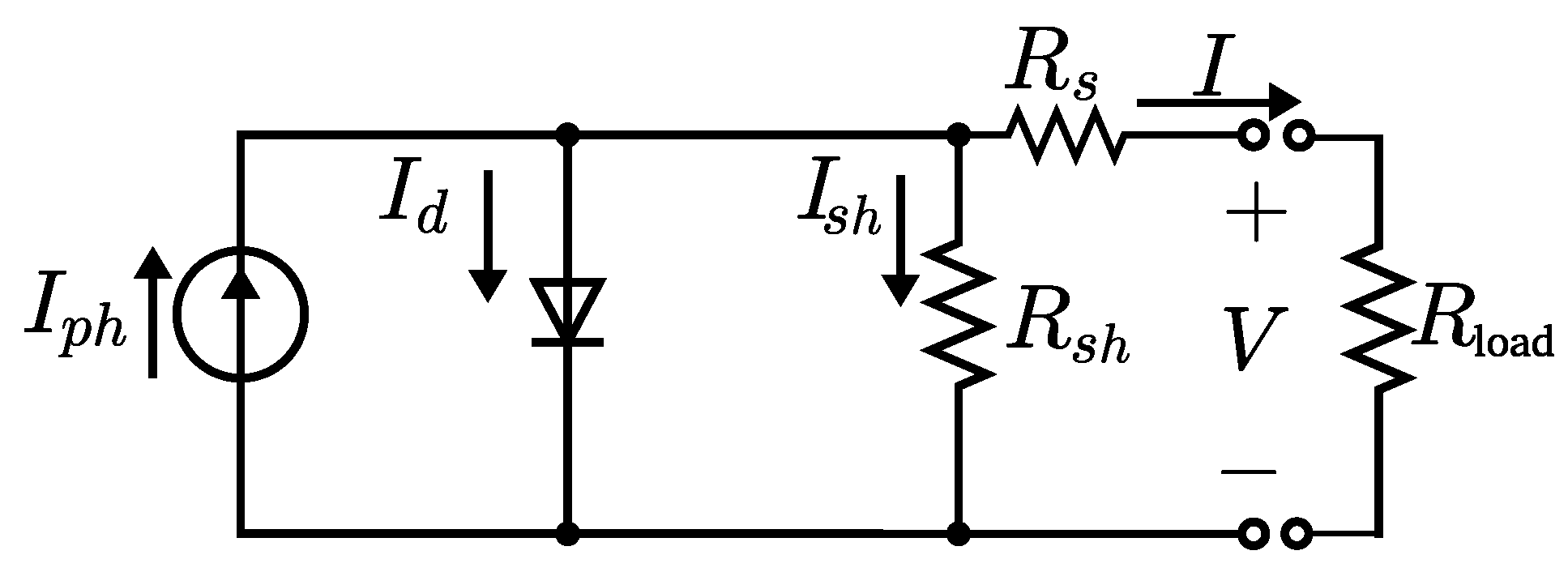Each model has its own parameters, in such a way that it is necessary to find the set of values which minimizes the error between the measured and the simulated I–V curves. For the SDM, these parameters are the photo-generated current $I_{ph}$, the dark-saturation current $I_s$, the diode ideality/quality factor m, the series resistance $R_s$, and shunt/parallel resistance $R_{sh}$. The SDM equivalent circuit can be seen in Figure 1, whereas (Equation (9)) describes its electrical behavior:

$$I=I_L-I_s·\left[exp\left(\frac{V+I·R_s}{{\mathrm{N}}_{\mathrm{s}}·m·V_{th}}\right)-1\right]-\frac{V+I·R_s}{R_{sh}}$$

(9)

where ${\mathrm{N}}_{\mathrm{s}}$ is the number of cells in series, and $V_{th}=\mathrm{k}·T/\mathrm{q}$ is the thermal voltage, being $\mathrm{k}=1.380649 \times {10}^{-23}$ J/K (the Boltzmann constant) and $\mathrm{q}=1.602176634 \times {10}^{-19}$ C (the elementary charge). Herein, T is assumed to be expressed in kelvin.

The expression in (Equation (9)) must be satisfied for every point $(V_1^{\left(j\right)},I_1^{\left(j\right)})$ of the initial curve, and the obtained parameters $(I_{ph1},I_{s1},m_1,R_{s1},R_{sh1})$ are assumed to refer to the set of conditions $(G_1,T_1)$. Some of these parameters can be assumed as internal constants of the device, but others can be dependent on the irradiance $G_1$ and/or the cell temperature $T_1$. For example, it is possible to find in the literature [16,17,18] expressions matching (Equations (10)–(13)), to translate the variable parameters from the initial conditions $(G_1,T_1)$ to the target conditions $(G_2,T_2)$. Often these formula require knowing beforehand a few additional intrinsic coefficients, such as $\alpha$ (the temperature coefficient of $I_{\mathrm{SC}}$) or $E_g$ (the energy band-gap of the semi-conductor material), which could be provided by the manufacturer or generic values for each PV technology can be taken from the literature.

$$\begin{array}{c}{I}_{ph2}=\mathcal{F}\left(I_{ph1},G_1,T_1,G_2,T_2,\alpha ,\dots \right)\end{array}$$

(10)

$$\begin{array}{c}{I}_{s2}=\mathcal{G}\left(I_{s1},G_1,T_1,G_2,T_2,E_g,\dots \right)\end{array}$$

(11)

$$\begin{array}{c}{R}_{s2}=\mathcal{H}\left(R_{s1},G_1,T_1,G_2,T_2,\nu ,\dots \right)\end{array}$$

(12)

$$\begin{array}{c}{R}_{sh2}=\mathcal{I}\left(R_{sh1},G_1,T_1,G_2,T_2,\lambda ,\dots \right)\end{array}$$

(13)

Therefore, the model represented by (Equation (9)) can be adjusted for the I–V pairs using a curve-fitting routine included in any mathematical suite such as Matlab [19], which takes as input a matrix with all the points $(V_1^{\left(j\right)},I_1^{\left(j\right)})$ and returns as output the required parameters, $(I_{ph1},I_{s1},m,R_{s1},R_{sh1},\dots )$ referring to the initial conditions $(G_1,T_1)$. The next step is to translate the parameters from those conditions into the target conditions $(G_2,T_2)$ by means of equations from (Equations (10) to (13)). Finally, it is possible to generate an I–V curve at the irradiance $G_2$ and temperature $T_2$, defining a mesh of voltage points and substituting each coordinate value in (Equation (9)) to obtain its current image, eventually having the full simulated I–V curve.

D.

DDM-based Numerical Methods

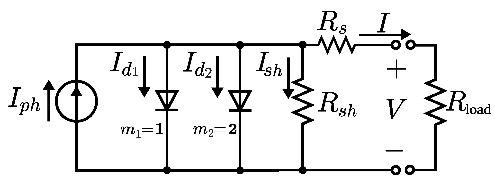
A similar approach to the previous one can be followed if the DDM equivalent circuit is taken as the underlying model. In that case, an expression like (Equation (14)) is assumed by many authors [20,21,22,23], using two exponential elements (see Figure 2), in such a way that the first diode (with $m_1=1$) takes into account the phenomena in the quasi-neutral region, whereas the second diode (with $m_2=2$) is related to the carrier recombination in the space-charge region [24].

$$I=I_{ph}-I_{s1}·\left[exp\left(\frac{V+I·R_s}{{\mathrm{N}}_{\mathrm{s}}·m_1·V_{th}}\right)-1\right]-I_{s2}·\left[exp\left(\frac{V+I·R_s}{{\mathrm{N}}_{\mathrm{s}}·m_2·V_{th}}\right)-1\right]-\frac{V+I·R_s}{R_{sh}}$$

(14)

where there are two dark saturation current values $I_{s1}$ and $I_{s2}$ to determine, in such a way that there are two different expressions used to translate the values from the initial conditions $(G_1,T_1)$ to the target conditions $(G_2,T_2)$ (in addition to the other translation equations). In its initial formulation, this model has five parameters to be estimated, but some authors have proposed alternative approaches, where $m_1$ and/or $m_2$ are also free parameters to be adjusted.

E.

Analytical Methods

The methods in this group are also based on physical models of the solar cell, and again the goal is the determination of the parameters $(I_{ph1},I_{s1},m,R_{s1},R_{sh1},\dots )$ referring to the initial conditions $(G_1,T_1)$ and their subsequent correction to $(I_{ph2},I_{s2},m,R_{s2},R_{sh2},\dots )$ associated with the target conditions $(G_2,T_2)$, and finally the simulation of the I–V curve for these latter conditions (assuming m as a constant intrinsic parameter). However, instead of using as input all the discrete points of the I–V curve, the optimization routine uses as input the values of the main electrical parameters and the slopes of the curve at certain specific points.

The underlying model (valid for all the points of the I–V curve) is instantiating for some special conditions. In this way, it is possible to obtain a particular expression (that depends on the required parameters) valid only at the “short-circuit” point, and another one only for the “open-circuit” condition, and so on. Eventually, it is necessary to obtain a number of equations equal to the number of free parameters, in order to obtain a system of equations with a unique solution. As those equations will be non-linear, it is necessary to use complex system solver routines, which require significant hardware resources.

Once the system of equations has been solved, the parameters for the initial conditions $(G_1,T_1)$ are corrected to the target conditions $(G_2,T_2)$, and finally the I–V curve under those conditions can be reconstructed. The fundamental difference with type C or type D methods is that it is not necessary to fit all the points of the initial I–V curve to the underlying model to determine the parameters, but they are instead determined only from the main electrical parameters and perhaps from a few other values that can be estimated from the I–V curve.

F.

Explicit Methods

Along the same line as the previous group, this type also includes some methods based on the main electrical parameters of the I–V measured under the initial conditions. However, in order to avoid having to solve a non-linear system of equations, a few reasonable assumptions are applied to perform various algebraic manipulations, obtaining at the end a series of explicit expressions used to determine all the required parameters, requiring a low computational burden [25,26,27]. A review of these explicit methods is provided by Batzelis [28].

Once the required parameters have been determined and corrected to the target conditions, the underlying model is used to reconstruct the curve under the new measurement conditions. Instead of using the generic non-explicit model, it is common in this type of methods to use fast alternative approaches to also reconstruct the I–V curve. For example, a reformulation of the underlying model defined in (Equation (9)) can be made by means of the W–Lambert function [26], in such a way that each current coordinate can be obtained explicitly from the value of the voltage coordinate and the other parameters determined previously.

G.

Iterative Methods

Analogously to the previous type, most of the parameters required by the underlying model can be estimated using explicit expressions from the main electrical parameters. However, one parameter (or perhaps a couple of them) must be determined by means of a simple and fast iterative routine that finishes when the simulated curve satisfies a predefined criterion. Alternatively, in some approaches, some of the parameters to be determined must be known beforehand, so a method to determine only that parameter should be executed beforehand.

H.

Interpolation Methods

In the previous categories of methods, only a unique initial I–V curve is used as input to generate the target I–V curve under the final conditions. Type H approaches, on the other hand, allow combining a few initial curves referring to the conditions $(G_{1a},T_{1a})$, $(G_{1b},T_{1b})$, …, to obtain an output curve associated with the target irradiance and temperature $(G_2,T_2)$. In this type of method, the new I–V curve is obtained by means of an interpolation of the points of the different initial curves used as inputs. One drawback is that these interpolation methods cannot be applied to every set of initial curves. It is necessary to find a combination of initial curves satisfying certain criteria. Another disadvantage can arise when the target conditions are beyond the interval defined by the initial conditions. In these cases, it is not an interpolation but actually an extrapolation, which can lead to high errors [29,30].

1.2. Correction Procedures

Table 1 summarizes all the studied and implemented methods, classifying them into one of the previous eight categories (A, B, C, D, E, F, G, or H). For each method, a list of the required intrinsic coefficients is also included. In order to clarify the meaning of the coefficients, Table 2 includes a row for each required intrinsic coefficient, as well as providing a reference with a method to estimate its value, if this is not provided by the manufacturer. In the rest of this section, every studied approach will be briefly explained, providing the equations to be applied.

A01:

BASIC method

This method obtains $I_{\mathrm{SC}2}$ from $I_{\mathrm{SC}1}$, taking into account the definition of the temperature coefficient $\alpha$ and the linear effect of the irradiance on the short-circuit current [31], as can be seen in (Equation (15)). Herein, $\alpha$ refers to the target irradiance $G_2$ (as stated by King et al. [32], $\alpha$ depends on the irradiance):

$$I_{\mathrm{SC}2}=\frac{G_2}{G_1}·I_{\mathrm{SC}1}+\alpha \left(G_2\right)·(T_2-T_1)$$

(15)

Alternatively, an equivalent formula (Equation (16)) can be found throughout the literature [9,33,34]:

$$I_{\mathrm{SC}2}=\frac{G_2}{G_1}·I_{\mathrm{SC}1}·\left[1+{\alpha }_r·(T_2-T_1)\right]$$

(16)

where ${\alpha }_r$ is the relative temperature coefficient of the short-circuit current, expressed in 1/K (this does not depend on G).

In order to obtain $V_{\mathrm{OC}2}$ for the target conditions $(G_2,T_2)$ from the value of $V_{\mathrm{OC}1}$ under the initial conditions $(G_1,T_1)$, (Equation (17)) can be directly applied [9,35,36]:

$$V_{\mathrm{OC}2}=V_{\mathrm{OC}1}+\beta ·(T_2-T_1)$$

(17)

where $\beta$ is the temperature coefficient of the open-circuit voltage $V_{\mathrm{OC}}$, given by the manufacturer or estimated from experimental data. Finally, to translate the full I–V curve, (Equation (4)) can be applied to each discrete point.

Table 1. Summary of the methods used to translate I–V curves.

Id.  –  Abbr.		Method	Ref.	Parameters
A01	BASIC	BASIC method	[9]	$\alpha$, $\beta$
A02	RBACH	Method of Rauschenbach	[31]	$\alpha$, $\beta$, $R_S$
A03	CASTAÑER	Method of Castañer	[37]	$\alpha$, $\beta$, m
A04	REDDY	Method of Reddy	[38]	${\alpha }_r$, ${\beta }_r$, $\delta$
A05	ANDERSON	Method of Anderson	[4]	${\alpha }_r,{\beta }_r,{\gamma }_r,\delta$
A06	SMITH	Method of Smith	[10]	${\alpha }_r$, ${\beta }_r$, ${\gamma }_r$
A07	CARRILLO	Method of Carrillo	[39]	${\alpha }_r$, ${\beta }_r$
A08	DIA	Method of Dia	[40]	${\alpha }_r$, $\beta$
A09	ZHOU	Method of Zhou-Dongue	[41]	$\alpha$, $\delta$, $\xi$, $\chi$
A10	BATZELIS(a)	Method of Batzelis (a)	[13]	${\alpha }_r$, ${\beta }_r$
B01	BLAESSER	Method of Blaesser	[42]	$\alpha$, $\beta$, m
B02	ALONSO	Method of Alonso-Abella	[43]	$\alpha$, $\beta$, m
B03	JRC	JRC method	[44]	${\alpha }_r$, ${\beta }_r$, $R_s$, $\delta$
B04	IEC-P1	IEC 60891:2021 P1	[3]	$\alpha$, $\beta$, $R_s$, $\kappa$
B05	IEC-P1(b)	Simplified IEC 60891 P1	[45]	$\alpha$, $\beta$
B06	IEC-P2	IEC 60891:2009 P2	[46]	${\alpha }_r$, ${\beta }_r$, $R_s$,$\kappa$, $\delta$
B07	IEC-P2(b)	Modified IEC 60891 P2	[47]	${\alpha }_r$, ${\beta }_r$, $R_s$,$\kappa$, $\delta$
B08	IEC-P2(c)	IEC 60891:2021 P2	[3]	${\alpha }_r$, ${\beta }_r$, $R_s$, $\kappa$, ${\delta }_1$, ${\delta }_2$
B09	IEC-P4	IEC 60891:2021 P4	[3]	${\alpha }_r$, $R_s$, $\epsilon$
B10	IEC-P4(b)	IEC60891:2021 P4 (mod)	[3]	${\alpha }_r$, $R_s$, $m,E_g$
C01	ISDM	Ideal single-diode model	[48]	$\alpha$, $E_g$
C02	SSDM	Simplified single-diode	[49]	$\alpha$, $E_g$
C03	SDM	Single-diode model	[50]	$\alpha$, $E_g$
C04	SDM(b)	Single-diode model (b)	[51]	$\alpha$, $E_g$
C05	RUSCHELL	Equation of Ruschell	[18]	$\alpha$, $E_g,\eta ,\lambda$
C06	PVSYST	PVsyst method	[52]	$\alpha$, $E_g,\mu ,\nu$
C07	WALKER	Expression of Walker	[53]	$\alpha$, $E_g$, $\mu ,\nu$
C08	LAURINO	Equations of Laurino	[54]	$\alpha$, $E_g$, $\mu ,\nu ,\kappa$
C09	DING	Expression of Ding	[55]	$\alpha$, $E_g$, $\mu ,\nu ,B_s$
C10	COTFAS	Equations of Cotfas	[56]	$\alpha$, $E_g$, $\mu ,\nu$
C11	SSDM *	Modified SSDM	[49]	$\alpha$, $E_g$, $\xi$
C12	SDM *	Modified SDM	[50]	$\alpha$, $E_g,\xi$
C13	PVSYST *	PVSYST method (mod)	[52]	$\alpha$, $E_g$, $\mu ,\nu ,\xi$
C14	WALKER *	Walker’s method (mod)	[53]	$\alpha$, $E_g$, $\mu ,\nu ,\xi$
C15	LAURINO *	Laurino’s method (mod)	[54]	$\alpha ,E_g$, $\mu ,\nu ,\kappa ,\xi$
D01	SDDM	Simplified double-diode	[49]	$\alpha$, $E_g$
D02	DDM-5p	Double-diode (5 par)	[57]	$\alpha$, $E_g$
D03	DDM-6p	Double-diode (6 par)	[58]	$\alpha$, $E_g$
D04	DDM-7p	Double-diode (7 par)	[20]	$\alpha$, $E_g$
D05	SDDM *	Modified SDDM	[49]	$\alpha$, $E_g,\xi$
D06	DDM-5p *	Modified DDM-5p	[57]	$\alpha$, $E_g$, $\mu ,\nu ,\xi$
D07	DDM-6p *	Modified DDM-6p	[58]	$\alpha$, $E_g$, $\mu ,\nu ,\xi$
D08	DDM-7p *	Modified DDM-7p	[20]	$\alpha$, $E_g$, $\mu ,\nu ,\xi$
E01	LOBRANO	Model of Lo Brano	[59]	$\alpha$, $\beta$
E02	SERA	Model of Sera	[60]	$\alpha$, $\beta$
E03	ORIOLI	Model of Orioli	[61]	${\alpha }_r$, ${\beta }_r$
E04	DeSOTO	Method of De Soto	[62]	$\alpha$, $\beta$
E05	TOLEDO	Model of Toledo	[63]	$\alpha$, $\beta$
E06	XIAO	Method of Xiao	[35]	$\alpha$, $E_g$
E07	LoBRANO *	Modified Lo Brano’s	[59]	$\alpha$, $\beta$, $\xi$
E08	SERA *	Modified Sera’s	[60]	$\alpha$, $\beta$, $\xi$
E09	ORIOLI *	Modified Orioli’s	[61]	${\alpha }_r$, ${\beta }_r$, $\xi$
E10	DeSOTO *	Modified De Soto’s	[62]	$\alpha$, $\beta$, $\xi$
E11	TOLEDO *	Modified Toledo’s	[63]	$\alpha$, $\beta$, $\xi$
E12	XIAO *	Modified Xiao’s	[35]	$\alpha$, $E_g$, $\xi$
F01	SALOUX	Method of Saloux	[64]	$\alpha$, $E_g$
F02	PHANG	Method of Phang	[25]	$\alpha$, $E_g$
F03	CUBAS(a)	Method of Cubas (a)	[65]	$\alpha$, $E_g$
F04	CUBAS(b)	Method of Cubas (b)	[65]	$\alpha$, $E_g$
F05	CUBAS(c)	Method of Cubas (c)	[66]	$\alpha$, m, $E_g$
F06	KHAN	Method of Khan	[67]	$\alpha$, $E_g$
F07	PETRONE	Method of Petrone	[26]	$\alpha$, $\beta$, $E_g$
F08	SPRATIO	SPR method	[68]	$\alpha$, $E_g$
F09	BAI	Method of Bai	[69]	$\alpha$, $E_g$
F10	CRISTALDI	Method of Cristaldi	[70]	${\alpha }_r$, ${\beta }_r$
F11	SERA(b)	Explicit Sera’s method	[71]	$\alpha$, $E_g$
F12	TOLEDO(b)	Explicit Toledo’s method	[72]	$\alpha$, $E_g$
F13	BATZELIS(b)	Batzelis’ method (b)	[13]	${\alpha }_r$, ${\beta }_r$, $E_g$
F14	SALOUX *	Modified Saloux’	[64]	$\alpha$, $E_g$, $\xi$
F15	PHANG *	Modified Phang’s	[25]	$\alpha$, $E_g$, $\xi$
F16	CUBAS(a) *	Modified Cubas’s (a)	[65]	$\alpha$, $E_g$, $\xi$
F17	CUBAS(b) *	Modified Cubas’s (b)	[65]	$\alpha$, $E_g$, $\xi$
F18	CUBAS(c) *	Modified Cubas’s (c)	[66]	$\alpha$, m,$\xi$, $E_g$
F19	KHAN *	Modified Khan’s	[67]	$\alpha$, $E_g$, $\xi$
F20	PETRONE *	Modified Petrone’s	[26]	$\alpha ,\beta$, $\xi ,E_g$
F21	SPRATIO *	Modified SPR method	[68]	$\alpha ,\beta$, $\xi ,E_g$
F22	BAI *	Modified Bai’s	[69]	$\alpha$, $E_g$, $\xi$
F23	CRISTALDI *	Modified Cristaldi’s	[70]	${\alpha }_r$, ${\beta }_r$, $\xi$
F24	SERA(b) *	Modified explicit Sera’s	[71]	$\alpha$, $E_g$, $\xi$
F25	TOLEDO(b) *	Modified explicit Toledo’s	[72]	$\alpha$, $E_g$, $\xi$
F26	BATZELIS(b) *	Modified Batzelis’ (b)	[13]	${\alpha }_r$, ${\beta }_r$, $\xi$, $E_g$
G01	VILLALVA	Model of Villalva	[16]	$\alpha$, $\beta$, m
G02	BOUTANA	Model of Boutana	[73]	$\alpha$, m, $E_g$
G03	CARRERO	Model of Carrero	[74]	$\alpha$, $E_g$
G04	STORNELLI	Method of Stornelli	[75]	$\alpha$, $E_g$
G05	VILLALVA *	Modified Villalva’s	[16]	$\alpha$, $\beta$, m, $\xi$
G06	BOUTANA *	Modified Boutana’s	[73]	$\alpha$, $\beta$, m, $\xi$
G07	CARRERO *	Modified Carrero’s	[74]	$\alpha$, $\beta$, m, $\xi$
G08	STORNELLI *	Modified Stornelli’s	[75]	$\alpha$, $\beta$, $\xi$
H01	LINEAR	Linear interpolation		None
H02	BILINEAR	Bilinear interpolation	[7]	None
H03	IEC-P3	IEC 60891:2021 P3	[3]	None

* Each of these methods is identical to the original approach, except for using the fitting parameter ξ included in (Equation (29)).

Table 1. Summary of the methods used to translate I–V curves.

Id.  –  Abbr.		Method	Ref.	Parameters
A01	BASIC	BASIC method	[9]	$\alpha$, $\beta$
A02	RBACH	Method of Rauschenbach	[31]	$\alpha$, $\beta$, $R_S$
A03	CASTAÑER	Method of Castañer	[37]	$\alpha$, $\beta$, m
A04	REDDY	Method of Reddy	[38]	${\alpha }_r$, ${\beta }_r$, $\delta$
A05	ANDERSON	Method of Anderson	[4]	${\alpha }_r,{\beta }_r,{\gamma }_r,\delta$
A06	SMITH	Method of Smith	[10]	${\alpha }_r$, ${\beta }_r$, ${\gamma }_r$
A07	CARRILLO	Method of Carrillo	[39]	${\alpha }_r$, ${\beta }_r$
A08	DIA	Method of Dia	[40]	${\alpha }_r$, $\beta$
A09	ZHOU	Method of Zhou-Dongue	[41]	$\alpha$, $\delta$, $\xi$, $\chi$
A10	BATZELIS(a)	Method of Batzelis (a)	[13]	${\alpha }_r$, ${\beta }_r$
B01	BLAESSER	Method of Blaesser	[42]	$\alpha$, $\beta$, m
B02	ALONSO	Method of Alonso-Abella	[43]	$\alpha$, $\beta$, m
B03	JRC	JRC method	[44]	${\alpha }_r$, ${\beta }_r$, $R_s$, $\delta$
B04	IEC-P1	IEC 60891:2021 P1	[3]	$\alpha$, $\beta$, $R_s$, $\kappa$
B05	IEC-P1(b)	Simplified IEC 60891 P1	[45]	$\alpha$, $\beta$
B06	IEC-P2	IEC 60891:2009 P2	[46]	${\alpha }_r$, ${\beta }_r$, $R_s$,$\kappa$, $\delta$
B07	IEC-P2(b)	Modified IEC 60891 P2	[47]	${\alpha }_r$, ${\beta }_r$, $R_s$,$\kappa$, $\delta$
B08	IEC-P2(c)	IEC 60891:2021 P2	[3]	${\alpha }_r$, ${\beta }_r$, $R_s$, $\kappa$, ${\delta }_1$, ${\delta }_2$
B09	IEC-P4	IEC 60891:2021 P4	[3]	${\alpha }_r$, $R_s$, $\epsilon$
B10	IEC-P4(b)	IEC60891:2021 P4 (mod)	[3]	${\alpha }_r$, $R_s$, $m,E_g$
C01	ISDM	Ideal single-diode model	[48]	$\alpha$, $E_g$
C02	SSDM	Simplified single-diode	[49]	$\alpha$, $E_g$
C03	SDM	Single-diode model	[50]	$\alpha$, $E_g$
C04	SDM(b)	Single-diode model (b)	[51]	$\alpha$, $E_g$
C05	RUSCHELL	Equation of Ruschell	[18]	$\alpha$, $E_g,\eta ,\lambda$
C06	PVSYST	PVsyst method	[52]	$\alpha$, $E_g,\mu ,\nu$
C07	WALKER	Expression of Walker	[53]	$\alpha$, $E_g$, $\mu ,\nu$
C08	LAURINO	Equations of Laurino	[54]	$\alpha$, $E_g$, $\mu ,\nu ,\kappa$
C09	DING	Expression of Ding	[55]	$\alpha$, $E_g$, $\mu ,\nu ,B_s$
C10	COTFAS	Equations of Cotfas	[56]	$\alpha$, $E_g$, $\mu ,\nu$
C11	SSDM *	Modified SSDM	[49]	$\alpha$, $E_g$, $\xi$
C12	SDM *	Modified SDM	[50]	$\alpha$, $E_g,\xi$
C13	PVSYST *	PVSYST method (mod)	[52]	$\alpha$, $E_g$, $\mu ,\nu ,\xi$
C14	WALKER *	Walker’s method (mod)	[53]	$\alpha$, $E_g$, $\mu ,\nu ,\xi$
C15	LAURINO *	Laurino’s method (mod)	[54]	$\alpha ,E_g$, $\mu ,\nu ,\kappa ,\xi$
D01	SDDM	Simplified double-diode	[49]	$\alpha$, $E_g$
D02	DDM-5p	Double-diode (5 par)	[57]	$\alpha$, $E_g$
D03	DDM-6p	Double-diode (6 par)	[58]	$\alpha$, $E_g$
D04	DDM-7p	Double-diode (7 par)	[20]	$\alpha$, $E_g$
D05	SDDM *	Modified SDDM	[49]	$\alpha$, $E_g,\xi$
D06	DDM-5p *	Modified DDM-5p	[57]	$\alpha$, $E_g$, $\mu ,\nu ,\xi$
D07	DDM-6p *	Modified DDM-6p	[58]	$\alpha$, $E_g$, $\mu ,\nu ,\xi$
D08	DDM-7p *	Modified DDM-7p	[20]	$\alpha$, $E_g$, $\mu ,\nu ,\xi$
E01	LOBRANO	Model of Lo Brano	[59]	$\alpha$, $\beta$
E02	SERA	Model of Sera	[60]	$\alpha$, $\beta$
E03	ORIOLI	Model of Orioli	[61]	${\alpha }_r$, ${\beta }_r$
E04	DeSOTO	Method of De Soto	[62]	$\alpha$, $\beta$
E05	TOLEDO	Model of Toledo	[63]	$\alpha$, $\beta$
E06	XIAO	Method of Xiao	[35]	$\alpha$, $E_g$
E07	LoBRANO *	Modified Lo Brano’s	[59]	$\alpha$, $\beta$, $\xi$
E08	SERA *	Modified Sera’s	[60]	$\alpha$, $\beta$, $\xi$
E09	ORIOLI *	Modified Orioli’s	[61]	${\alpha }_r$, ${\beta }_r$, $\xi$
E10	DeSOTO *	Modified De Soto’s	[62]	$\alpha$, $\beta$, $\xi$
E11	TOLEDO *	Modified Toledo’s	[63]	$\alpha$, $\beta$, $\xi$
E12	XIAO *	Modified Xiao’s	[35]	$\alpha$, $E_g$, $\xi$
F01	SALOUX	Method of Saloux	[64]	$\alpha$, $E_g$
F02	PHANG	Method of Phang	[25]	$\alpha$, $E_g$
F03	CUBAS(a)	Method of Cubas (a)	[65]	$\alpha$, $E_g$
F04	CUBAS(b)	Method of Cubas (b)	[65]	$\alpha$, $E_g$
F05	CUBAS(c)	Method of Cubas (c)	[66]	$\alpha$, m, $E_g$
F06	KHAN	Method of Khan	[67]	$\alpha$, $E_g$
F07	PETRONE	Method of Petrone	[26]	$\alpha$, $\beta$, $E_g$
F08	SPRATIO	SPR method	[68]	$\alpha$, $E_g$
F09	BAI	Method of Bai	[69]	$\alpha$, $E_g$
F10	CRISTALDI	Method of Cristaldi	[70]	${\alpha }_r$, ${\beta }_r$
F11	SERA(b)	Explicit Sera’s method	[71]	$\alpha$, $E_g$
F12	TOLEDO(b)	Explicit Toledo’s method	[72]	$\alpha$, $E_g$
F13	BATZELIS(b)	Batzelis’ method (b)	[13]	${\alpha }_r$, ${\beta }_r$, $E_g$
F14	SALOUX *	Modified Saloux’	[64]	$\alpha$, $E_g$, $\xi$
F15	PHANG *	Modified Phang’s	[25]	$\alpha$, $E_g$, $\xi$
F16	CUBAS(a) *	Modified Cubas’s (a)	[65]	$\alpha$, $E_g$, $\xi$
F17	CUBAS(b) *	Modified Cubas’s (b)	[65]	$\alpha$, $E_g$, $\xi$
F18	CUBAS(c) *	Modified Cubas’s (c)	[66]	$\alpha$, m,$\xi$, $E_g$
F19	KHAN *	Modified Khan’s	[67]	$\alpha$, $E_g$, $\xi$
F20	PETRONE *	Modified Petrone’s	[26]	$\alpha ,\beta$, $\xi ,E_g$
F21	SPRATIO *	Modified SPR method	[68]	$\alpha ,\beta$, $\xi ,E_g$
F22	BAI *	Modified Bai’s	[69]	$\alpha$, $E_g$, $\xi$
F23	CRISTALDI *	Modified Cristaldi’s	[70]	${\alpha }_r$, ${\beta }_r$, $\xi$
F24	SERA(b) *	Modified explicit Sera’s	[71]	$\alpha$, $E_g$, $\xi$
F25	TOLEDO(b) *	Modified explicit Toledo’s	[72]	$\alpha$, $E_g$, $\xi$
F26	BATZELIS(b) *	Modified Batzelis’ (b)	[13]	${\alpha }_r$, ${\beta }_r$, $\xi$, $E_g$
G01	VILLALVA	Model of Villalva	[16]	$\alpha$, $\beta$, m
G02	BOUTANA	Model of Boutana	[73]	$\alpha$, m, $E_g$
G03	CARRERO	Model of Carrero	[74]	$\alpha$, $E_g$
G04	STORNELLI	Method of Stornelli	[75]	$\alpha$, $E_g$
G05	VILLALVA *	Modified Villalva’s	[16]	$\alpha$, $\beta$, m, $\xi$
G06	BOUTANA *	Modified Boutana’s	[73]	$\alpha$, $\beta$, m, $\xi$
G07	CARRERO *	Modified Carrero’s	[74]	$\alpha$, $\beta$, m, $\xi$
G08	STORNELLI *	Modified Stornelli’s	[75]	$\alpha$, $\beta$, $\xi$
H01	LINEAR	Linear interpolation		None
H02	BILINEAR	Bilinear interpolation	[7]	None
H03	IEC-P3	IEC 60891:2021 P3	[3]	None

* Each of these methods is identical to the original approach, except for using the fitting parameter ξ included in (Equation (29)).

Table 2. List of commonly used temperature coefficients and other required parameters.

Symbol / Formula		Description	Unit	Reference
$\alpha =$	${\displaystyle \frac{\partial I_{\mathrm{SC}}}{\partial T}}$	Absolute variation in the short-circuit current $I_{\mathrm{SC}}$ with respect to the cell temperature	A/K	[3,76]
${\alpha }_r=$	${\displaystyle \frac{1}{I_{\mathrm{SC},\mathrm{STC}}}}·{\displaystyle \frac{\partial I_{\mathrm{SC}}}{\partial T}}$	Relative variation in the short-circuit current $I_{\mathrm{SC}}$ with respect to the cell temperature	1/K	[3,76]
$\beta =$	${\displaystyle \frac{\partial V_{\mathrm{OC}}}{\partial T}}$	Absolute variation in the open-circuit voltage $V_{\mathrm{OC}}$ with respect to the cell temperature	V/K	[3,76]
${\beta }_r=$	${\displaystyle \frac{1}{V_{\mathrm{OC},\mathrm{STC}}}}·{\displaystyle \frac{\partial V_{\mathrm{OC}}}{\partial T}}$	Relative variation in the open-circuit voltage $V_{\mathrm{OC}}$ with respect to the cell temperature	1/K	[3,76]
$\gamma =$	${\displaystyle \frac{\partial P_{\mathrm{M}}}{\partial T}}$	Absolute variation in the maximum power $P_{\mathrm{M}}$ with respect to the cell temperature	W/K	[3,76]
${\gamma }_r=$	${\displaystyle \frac{1}{P_{\mathrm{M},\mathrm{STC}}}}·{\displaystyle \frac{\partial P_{\mathrm{M}}}{\partial T}}$	Relative variation in the maximum power $P_{\mathrm{M}}$ with respect to the cell temperature	1/K	[3,76]
$R_{\mathrm{S}1}=$	$R_{\mathrm{S},\mathrm{STC}}+\kappa ·(T_1-{\mathrm{T}}_{\mathrm{STC}})$	Internal series resistance of the device at the initial temperature $T_1$	$\Omega$	[77]
$\kappa =$	${\displaystyle \frac{\partial R_{\mathrm{S}}}{\partial T}}$	Absolute variation in the internal series resistance $R_{\mathrm{S}}$ with respect to the cell temperature	$\Omega$/K	[77]
$\delta$|	${\displaystyle \frac{V_{\mathrm{OC},\mathrm{STC}}}{V_{\mathrm{OC}}}}=1+\delta ·ln\left({\displaystyle \frac{{\mathrm{G}}_{\mathrm{STC}}}{G}}\right)$	Irradiance correction factor of the open-circuit voltage $V_{\mathrm{OC}}$ assuming a linear dependence	–	[46]
${\delta }_1=$	${\displaystyle \frac{\partial (V_{\mathrm{OC},\mathrm{STC}}/V_{\mathrm{OC}})}{\partial ({\mathrm{G}}_{\mathrm{STC}}/G)}}$	First-order correction factor of the open-circuit voltage $V_{\mathrm{OC}}$ assuming a quadratic dependence	–	[3]
${\delta }_2=$	${\displaystyle \frac{{\partial }^2(V_{\mathrm{OC},\mathrm{STC}}/V_{\mathrm{OC}})}{\partial {({\mathrm{G}}_{\mathrm{STC}}/G)}^2}}$	Second-order correction factor of the open–circuit voltage $V_{\mathrm{OC}}$ assuming a quadratic dependence	–	[3]
m		Diode ideality factor of the device	–	[78]
$E_g=$	$E_{g0\mathrm{K}}-{\displaystyle \frac{{\rho }_A·T^2}{T+{\rho }_B}}$	Band-gap energy of the semiconductor material at the actual temperature T	eV	[79]
$E_{g0\mathrm{K}}$		Band-gap energy of the semiconductor material at 0 K	eV	[79]
${\rho }_A$		Constant required by (Equation (74)) to estimate $E_g$	eV/K	[79]
${\rho }_B$		Constant required by (Equation (74)) to estimate $E_g$	K	[79]
$\xi =$	$\mathrm{mean}\left\{ln\left({\displaystyle \frac{I_{\mathrm{SC}}(G_i,T)}{I_{\mathrm{SC}}({\mathrm{G}}_{\mathrm{STC}},T)}}\right)/ln\left({\displaystyle \frac{G_i}{{\mathrm{G}}_{\mathrm{STC}}}}\right)\right\}$	Fitting parameter that accounts for the possible non-linearity of current with respect to the irradiance (estimated using curves at the same temperature)	–	[80]
$\chi$ =	$\mathrm{mean}\left\{ln\left({\displaystyle \frac{V_{\mathrm{OC}}(G,T_i)}{V_{\mathrm{OC}}(G,{\mathrm{T}}_{\mathrm{STC}})}}\right)/ln\left({\displaystyle \frac{{\mathrm{T}}_{\mathrm{STC}}}{T_i}}\right)\right\}$	Fitting parameter that accounts for the possible non-linearity of voltage with respect to the temperature (estimated using curves at the same irradiance)	–	[80]
$\eta$		Constant required by (Equation (82)) to estimate $R_{sh}$	–	[18]
$\lambda$		Constant required by (Equation (82)) to estimate $R_{sh}$	–	[18]
$\mu$		Constant required by (Equation (83)) to estimate $R_{sh}$	–	[52]
$\nu$		Constant required by (Equation (83)) to estimate $R_{sh}$	–	[52]
$\mathcal{R}$		Constant required by (Equation (84)) to estimate $R_{sh}$	–	[18]
$B_s$		Fitting parameter required by (Equation (86)) to estimate $R_s$	–	[55]

Table 2. List of commonly used temperature coefficients and other required parameters.

Symbol / Formula		Description	Unit	Reference
$\alpha =$	${\displaystyle \frac{\partial I_{\mathrm{SC}}}{\partial T}}$	Absolute variation in the short-circuit current $I_{\mathrm{SC}}$ with respect to the cell temperature	A/K	[3,76]
${\alpha }_r=$	${\displaystyle \frac{1}{I_{\mathrm{SC},\mathrm{STC}}}}·{\displaystyle \frac{\partial I_{\mathrm{SC}}}{\partial T}}$	Relative variation in the short-circuit current $I_{\mathrm{SC}}$ with respect to the cell temperature	1/K	[3,76]
$\beta =$	${\displaystyle \frac{\partial V_{\mathrm{OC}}}{\partial T}}$	Absolute variation in the open-circuit voltage $V_{\mathrm{OC}}$ with respect to the cell temperature	V/K	[3,76]
${\beta }_r=$	${\displaystyle \frac{1}{V_{\mathrm{OC},\mathrm{STC}}}}·{\displaystyle \frac{\partial V_{\mathrm{OC}}}{\partial T}}$	Relative variation in the open-circuit voltage $V_{\mathrm{OC}}$ with respect to the cell temperature	1/K	[3,76]
$\gamma =$	${\displaystyle \frac{\partial P_{\mathrm{M}}}{\partial T}}$	Absolute variation in the maximum power $P_{\mathrm{M}}$ with respect to the cell temperature	W/K	[3,76]
${\gamma }_r=$	${\displaystyle \frac{1}{P_{\mathrm{M},\mathrm{STC}}}}·{\displaystyle \frac{\partial P_{\mathrm{M}}}{\partial T}}$	Relative variation in the maximum power $P_{\mathrm{M}}$ with respect to the cell temperature	1/K	[3,76]
$R_{\mathrm{S}1}=$	$R_{\mathrm{S},\mathrm{STC}}+\kappa ·(T_1-{\mathrm{T}}_{\mathrm{STC}})$	Internal series resistance of the device at the initial temperature $T_1$	$\Omega$	[77]
$\kappa =$	${\displaystyle \frac{\partial R_{\mathrm{S}}}{\partial T}}$	Absolute variation in the internal series resistance $R_{\mathrm{S}}$ with respect to the cell temperature	$\Omega$/K	[77]
$\delta$|	${\displaystyle \frac{V_{\mathrm{OC},\mathrm{STC}}}{V_{\mathrm{OC}}}}=1+\delta ·ln\left({\displaystyle \frac{{\mathrm{G}}_{\mathrm{STC}}}{G}}\right)$	Irradiance correction factor of the open-circuit voltage $V_{\mathrm{OC}}$ assuming a linear dependence	–	[46]
${\delta }_1=$	${\displaystyle \frac{\partial (V_{\mathrm{OC},\mathrm{STC}}/V_{\mathrm{OC}})}{\partial ({\mathrm{G}}_{\mathrm{STC}}/G)}}$	First-order correction factor of the open-circuit voltage $V_{\mathrm{OC}}$ assuming a quadratic dependence	–	[3]
${\delta }_2=$	${\displaystyle \frac{{\partial }^2(V_{\mathrm{OC},\mathrm{STC}}/V_{\mathrm{OC}})}{\partial {({\mathrm{G}}_{\mathrm{STC}}/G)}^2}}$	Second-order correction factor of the open–circuit voltage $V_{\mathrm{OC}}$ assuming a quadratic dependence	–	[3]
m		Diode ideality factor of the device	–	[78]
$E_g=$	$E_{g0\mathrm{K}}-{\displaystyle \frac{{\rho }_A·T^2}{T+{\rho }_B}}$	Band-gap energy of the semiconductor material at the actual temperature T	eV	[79]
$E_{g0\mathrm{K}}$		Band-gap energy of the semiconductor material at 0 K	eV	[79]
${\rho }_A$		Constant required by (Equation (74)) to estimate $E_g$	eV/K	[79]
${\rho }_B$		Constant required by (Equation (74)) to estimate $E_g$	K	[79]
$\xi =$	$\mathrm{mean}\left\{ln\left({\displaystyle \frac{I_{\mathrm{SC}}(G_i,T)}{I_{\mathrm{SC}}({\mathrm{G}}_{\mathrm{STC}},T)}}\right)/ln\left({\displaystyle \frac{G_i}{{\mathrm{G}}_{\mathrm{STC}}}}\right)\right\}$	Fitting parameter that accounts for the possible non-linearity of current with respect to the irradiance (estimated using curves at the same temperature)	–	[80]
$\chi$ =	$\mathrm{mean}\left\{ln\left({\displaystyle \frac{V_{\mathrm{OC}}(G,T_i)}{V_{\mathrm{OC}}(G,{\mathrm{T}}_{\mathrm{STC}})}}\right)/ln\left({\displaystyle \frac{{\mathrm{T}}_{\mathrm{STC}}}{T_i}}\right)\right\}$	Fitting parameter that accounts for the possible non-linearity of voltage with respect to the temperature (estimated using curves at the same irradiance)	–	[80]
$\eta$		Constant required by (Equation (82)) to estimate $R_{sh}$	–	[18]
$\lambda$		Constant required by (Equation (82)) to estimate $R_{sh}$	–	[18]
$\mu$		Constant required by (Equation (83)) to estimate $R_{sh}$	–	[52]
$\nu$		Constant required by (Equation (83)) to estimate $R_{sh}$	–	[52]
$\mathcal{R}$		Constant required by (Equation (84)) to estimate $R_{sh}$	–	[18]
$B_s$		Fitting parameter required by (Equation (86)) to estimate $R_s$	–	[55]

A02:

Method of Rauschenbach

The main drawback of the previous approach is that it does not take into account the fact that a change in the short-circuit current can influence the open-circuit voltage because there is a parasitic series resistance $R_S$ whose value is not negligible. Rauschenbach [31], in addition to (Equation (15)), propose an alternative formula for $V_{\mathrm{OC}}$ (Equation (18)) that takes into account this effect:

$$V_{\mathrm{OC}2}=V_{\mathrm{OC}1}+\beta ·(T_2-T_1)-R_S·(I_{\mathrm{SC}2}-I_{\mathrm{SC}1})$$

(18)

A03:

Method of Castañer

This approach [37,81] tries to quantify the influence of the variation in the current on the open-circuit voltage by means of the thermal voltage $V_{th}$ (Equation (19)):

$$V_{\mathrm{OC}2}=V_{\mathrm{OC}1}+\beta ·(T_2-T_1)+{\mathrm{N}}_{\mathrm{s}}·m·V_{th2}·ln\left({\displaystyle \frac{I_{\mathrm{SC}2}}{I_{\mathrm{SC}1}}}\right)$$

(19)

A04:

Method of Reddy

Reddy et al. [38] took a method of type B (JRC method) and simplified it, using its basic equations to propose a pair of expressions to quantify $I_{\mathrm{SC}2}$ from $I_{\mathrm{SC}1}$ (the same Equation (16)) and $V_{\mathrm{OC}2}$ from $V_{\mathrm{OC}1}$ (Equation (20)):

$$V_{\mathrm{OC}2}=V_{\mathrm{OC}1}·\left[1+{\beta }_r·(T_2-T_1)+\delta ·ln\left({\displaystyle \frac{G_2}{G_1}}\right)\right]$$

(20)

where $\delta$ is known as the irradiance curve correction factor (in other references in the literature [46] the same parameter is noted as “a”). As can be seen, the effects of the temperature and irradiance are combined in an additive way.

A05:

Method of Anderson

Anderson [4,11] proposed (Equations (21)–(23)) to correct the main electrical parameters (this approach was also adopted in some early versions of ASTM E1036 [5]). The irradiance correction factor $\delta$ takes into account the effect of the irradiance on the voltage.

$$\begin{array}{cccc}\hfill & I_{\mathrm{SC}2}=I_{\mathrm{SC}1}·\frac{G_2}{G_1}·\frac{1}{1+{\alpha }_r·(T_1-T_2)}\hfill & \hfill & \end{array}$$

(21)

$$\begin{array}{cccc}\hfill & V_{\mathrm{OC}2}=V_{\mathrm{OC}1}·\frac{1}{1+{\beta }_r·(T_1-T_2)}·\frac{1}{1+\delta ·ln\left({\displaystyle \frac{G_1}{G_2}}\right)}\hfill & \hfill & \end{array}$$

(22)

$$\begin{array}{ccc}\hfill & P_{\mathrm{M}2}=P_{\mathrm{M}1}·\frac{G_2}{G_1}·\frac{1}{1+{\gamma }_r·(T_1-T_2)}·\frac{1}{1+\delta ·ln\left({\displaystyle \frac{G_1}{G_2}}\right)}\hfill & \hfill \end{array}$$

(23)

where ${\alpha }_r$, ${\beta }_r$ and ${\gamma }_r$ are the temperature coefficients of $I_{\mathrm{SC}}$, $V_{\mathrm{OC}}$ and $P_{\mathrm{M}}$, respectively. It must be highlighted that this method provides (Equation (23)), which estimates a value for the maximum power $P_{\mathrm{M}2}$ that is not necessarily equal to the one that can be obtained from the discrete points of the corrected curve obtained using (Equations (21) and (22)).

A06:

Method of Smith

Smith et al. [10] presented a simplification of the method of Anderson [4], giving three expressions: (Equations (24)–(26)). In this approach, only the three temperature coefficients provided by the manufacturer in the specification sheet are required:

$$\begin{array}{c}{I}_{\mathrm{SC}2}=I_{\mathrm{SC}1}·{\displaystyle \frac{G_2}{G_1}}·{\displaystyle \frac{1}{1+{\alpha }_r·(T_1-T_2)}}\end{array}$$

(24)

$$\begin{array}{c}{V}_{\mathrm{OC}2}=V_{\mathrm{OC}1}·\frac{1}{1+{\beta }_r·(T_1-T_2)}\end{array}$$

(25)

$$\begin{array}{c}{P}_{\mathrm{M}2}=P_{\mathrm{M}1}·\frac{G_2}{G_1}·\frac{1}{1+{\gamma }_r·(T_1-T_2)}\end{array}$$

(26)

As a third expression for obtaining $P_{\mathrm{M}2}$ is provided, it is possible to obtain different numerical values for that electrical parameter.

A07:

Method of Carrillo

Carrillo et al. [39] provided some expressions that with a notation change and a small work-around can be transformed into (Equations (27) and (28)) and can be used to translate the curves:

$$\begin{array}{c}{I}_{\mathrm{SC}2}=I_{\mathrm{SC}1}·\frac{G_2}{G_1}·\frac{1}{1+{\alpha }_r·(T_1-T_2)}\end{array}$$

(27)

$$\begin{array}{c}{V}_{\mathrm{OC}2}=\frac{V_{\mathrm{OC}1}+{\mathrm{N}}_{\mathrm{s}}·m·V_{th1}·ln\left({\displaystyle \frac{G_1}{G_2}}\right)}{1+{\beta }_r·(T_1-T_2)}\end{array}$$

(28)

A08:

Method of Dia

The approach presented by Dia et al. [40] is also named the “combination method”, because it uses (Equation (21)) to correct $I_{\mathrm{SC}}$ and the simple expression (Equation (17)) to correct $V_{\mathrm{OC}}$.

A09:

Method of Zhou–Dongue

Zhou et al. [80] proposed introducing two additional fitting parameters $\xi$ and $\chi$ (named $\alpha$ and $\gamma$ in the original paper) to deal with the possible non-linearity that affects the current and the voltage, respectively (see Table 2). As can be seen, to estimate $\xi$, a minimum of two different I–V curves are required, with equal temperature T (herein expressed in °C) but different irradiance values $G_i$. On the other hand, the estimation of $\chi$ involves two or more curves with common irradiance G and different temperature $T_i$.

Originally, the formula to correct $I_{\mathrm{SC}}$ does not take into account the temperature coefficient $\alpha$, but Dongue et al. [41] proposed an improvement in this line (Equation (29)). It must be highlighted that $\alpha$ refers to $G_1$, so the value ${\alpha }_{\mathrm{STC}}$ provided by the manufacturer must be scaled. In addition, the formula used to correct $V_{\mathrm{OC}}$ also includes the irradiance correction factor $\delta$ (Equation (30)):

$$\begin{array}{c}{I}_{\mathrm{SC}2}={\left(\frac{G_2}{G_1}\right)}^{\xi }·\left(I_{\mathrm{SC}1}+\alpha ·(T_2-T_1)\right)\end{array}$$

(29)

$$\begin{array}{c}{V}_{\mathrm{OC}2}={\left(\frac{T_1}{T_2}\right)}^{\chi }·\frac{V_{\mathrm{OC}1}}{1+\delta ·ln\left({\displaystyle \frac{G_1}{G_2}}\right)}\end{array}$$

(30)

A10:

Method of Batzelis

Batzelis [13] proposed a set of expressions (Equations (31)–(34)) to estimate the main electrical parameters at the target conditions:

$$\begin{array}{c}{I}_{\mathrm{SC}2}=I_{\mathrm{SC}1}·\frac{G_2}{G_1}·\left[1+{\alpha }_r·(T_2-T_1)\right]\end{array}$$

(31)

$$\begin{array}{c}{V}_{\mathrm{OC}2}=V_{\mathrm{OC}1}·\left[1+{\delta }_0·\frac{T_2}{T_1}·ln\left(\frac{G_2}{G_1}\right)+{\beta }_r·(T_2-T_1)\right]\end{array}$$

(32)

$$\begin{array}{c}{I}_{\mathrm{M}2}=I_{\mathrm{M}1}·\frac{G_2}{G_1}·\left[1+{\alpha }_{\mathrm{MPP}}·(T_2-T_1)\right]\end{array}$$

(33)

$$\begin{array}{c}{V}_{\mathrm{M}2}=V_{\mathrm{M}1}·\left[1+{\epsilon }_0·\frac{T_2}{T_1}·ln\left(\frac{G_2}{G_1}\right)+{\epsilon }_1·\left(1-\frac{G_2}{G_1}\right)+{\beta }_{\mathrm{MPP}}·(T_2-T_1)\right]\end{array}$$

(34)

These equations require several parameters that are usually unknown: ${\alpha }_{\mathrm{MPP}}$ (the relative temperature coefficient of $I_{\mathrm{M}}$), ${\beta }_{\mathrm{MPP}}$ (the relative temperature coefficient of $V_{\mathrm{M}}$), ${\delta }_0$ (the irradiance correction factor for $V_{\mathrm{OC}}$ evaluated in $T_1$), ${\epsilon }_0$ (a first irradiance correction factor for $V_{\mathrm{M}}$ evaluated in $T_1$), and ${\epsilon }_1$ (a second irradiance correction factor for $V_{\mathrm{M}}$, also referred to $T_1$). The method provides (Equations (35)–(40)) to calculate the additional parameters:

$$\begin{array}{cccc}\hfill & {\delta }_0=\frac{1-{\beta }_r·T_1}{50.1-{\alpha }_r·T_1}\hfill & \hfill & \hfill \end{array}$$

(35)

$$\begin{array}{cccc}\hfill & {\omega }_0=\mathcal{W}\left\{exp\left(\frac{1}{{\delta }_0}+1\right)\right\}\hfill & \hfill & \hfill \end{array}$$

(36)

$$\begin{array}{cccc}\hfill & {\epsilon }_0=\frac{{\delta }_0}{1+{\delta }_0}·{\displaystyle \frac{V_{\mathrm{OC}1}}{V_{\mathrm{M}1}}}\hfill & \hfill & \hfill \end{array}$$

(37)

$$\begin{array}{cccc}\hfill & {\epsilon }_1={\delta }_0·({\omega }_0-1)·{\displaystyle \frac{V_{\mathrm{OC}1}}{V_{\mathrm{M}1}}}-1\hfill & \hfill & \hfill \end{array}$$

(38)

$$\begin{array}{cccc}\hfill & {\alpha }_{\mathrm{MPP}}={\alpha }_r+{\displaystyle \frac{{\beta }_r-{\displaystyle \frac{1}{T_1}}}{{\omega }_0-1}}\hfill & \hfill & \hfill \end{array}$$

(39)

$$\begin{array}{cccc}\hfill & {\beta }_{\mathrm{MPP}}={\displaystyle \frac{V_{\mathrm{OC}1}}{V_{\mathrm{M}1}}}·\left[{\displaystyle \frac{{\beta }_r}{1+{\delta }_0}}+{\displaystyle \frac{{\delta }_0·({\omega }_0-1)-{\displaystyle \frac{1}{1+{\delta }_0}}}{T_1}}\right]\hfill & \hfill & \hfill \end{array}$$

(40)

where $\mathcal{W}\{·\}$ is the main branch ${\mathcal{W}}_0$ of the W–Lambert function [82].

Now, we will continue with the algebraic methods (including some ones described in IEC 60891:2021 [3]) that are the most used approaches for correcting I–V curves.

B01:

Method of Blaesser

According to Blaesser and Rossi [42], to correct an I–V curve measured at initial conditions $(G_1,T_1)$ to the new conditions $(G_2,T_2)$, the following steps can be carried out:

(a)

An auxiliary curve U (uncorrected) should be calculated, leaving the voltage component of each point j unchanged (Equation (41)) but applying a shift to the current component according to (Equation (42)):

$$\begin{array}{cccc}\hfill & V_U^{\left(j\right)}=V_1^{\left(j\right)}\hfill & \hfill & \end{array}$$

(41)

$$\begin{array}{ccc}\hfill & I_U^{\left(j\right)}=I_1^{\left(j\right)}+I_{\mathrm{SC},1}\left(\frac{G_2}{G_1}-1\right)+\alpha ·(T_2-T_1)\hfill & \hfill \end{array}$$

(42)

where $\alpha =(G_2/{\mathrm{G}}_{\mathrm{STC}})·{\alpha }_{\mathrm{STC}}$ refers to $G_2$ (scaling the value provided by the manufacturer) [83].

(b)

The short-circuit current $I_{\mathrm{SC},U}$ of the uncorrected curve must be determined by means of an interpolation [76] of the points around $V=0$. This $I_{\mathrm{SC},U}$ is already also the short-circuit current $I_{\mathrm{SC},2}$ of the final corrected curve.

(c)

In an analogous way, the open-circuit voltage $V_{\mathrm{OC},U}$ of the uncorrected curve is determined, again through interpolation [76] of the points around $I=0$.

(d)

The final value of the open-circuit voltage of the corrected curve should be estimated using (Equation (43)), where $V_{\mathrm{OC}1}$ is the open-circuit voltage of the original curve, $V_{th1}$ is the thermal voltage at the cell temperature $T_1$, ${\mathrm{N}}_{\mathrm{S}}$ is the number of cells in series, and m is the diode ideality factor.

$$V_{\mathrm{OC}2}=V_{\mathrm{OC}1}+\beta ·(T_2-T_1)+{\mathrm{N}}_{\mathrm{s}}·m·V_{th1}·ln\left({\displaystyle \frac{G_2}{G_1}}\right)$$

(43)

(e)

For each point j of the uncorrected curve U, a scaling is applied to the voltage component according to equation (Equation (45)), leaving the current component unchanged, thus obtaining the final corrected curve:

$$\begin{array}{ccc}\hfill I_2^{\left(j\right)}& =I_U^{\left(j\right)}\hfill & \end{array}$$

(44)

$$\begin{array}{ccc}\hfill V_2^{\left(j\right)}& =V_U^{\left(j\right)}·\left(\frac{V_{\mathrm{OC},2}}{V_{\mathrm{OC},U}}\right)\hfill & \hfill \end{array}$$

(45)

B02:

Method of Alonso–Abella

In this method [43], $I_{\mathrm{SC}2}$ and $V_{\mathrm{OC}2}$ corresponding to the corrected curve are first calculated, and then a succession of shifts are applied to fit the individual points, so that the new corrected curve intersects the axes precisely at those points. To correct the I–V from $(G_1,T_1)$ to $(G_2,T_2)$, we proceed as described below:

(a)

The values of $I_{\mathrm{SC}2}$ and $V_{\mathrm{OC}2}$ of the corrected curve are determined by means of (Equations (46) and (47)), assuming that $\alpha$ refers herein to $G_2$:

$$\begin{array}{cccc}\hfill & I_{\mathrm{SC}2}=I_{\mathrm{SC}1}·\left({\displaystyle \frac{G_2}{G_1}}\right)+\alpha ·(T_2-T_1)\hfill & \hfill & \end{array}$$

(46)

$$\begin{array}{ccc}\hfill & V_{\mathrm{OC}2}=V_{\mathrm{OC}1}+\beta ·(T_2-T_1)+{\mathrm{N}}_{\mathrm{s}}·m·V_{th1}·ln\left({\displaystyle \frac{G_2}{G_1}}\right)\hfill & \hfill \end{array}$$

(47)

(b)

For each point j of the original curve, the current component should be shifted by $\Delta I_{k=1}=I_{\mathrm{SC}2}-I_{\mathrm{SC}1}$ (where $k=1$ means that we are in the first iteration), without altering the voltage component (Equation (48)). This new auxiliary curve will pass through the point $(0,I_{\mathrm{SC}2})$:

$$I_{k=1}^{\left(j\right)}=I_1^{\left(j\right)}+\Delta I_{k=1}{V}_{k=1}^{\left(j\right)}=V_1^{\left(j\right)}$$

(48)

(c)

Based on the set of points of the curve of this iteration, its open-circuit voltage $V_{\mathrm{OC},k=1}$ is determined through interpolation [76] of the points around $I=0$.

(d)

The next step (iteration $k=2$) consists of applying another shift $\Delta V_{k=2}=V_{\mathrm{OC},2}-V_{\mathrm{OC},k=1}$ only on the voltage component of each point j, without altering the current component(Equation (49)). The obtained curve must necessarily pass through the point $(V_{\mathrm{OC},2},0)$:

$$V_{k=2}^{\left(j\right)}=V_{k=1}^{\left(j\right)}+\Delta V_{k=2}{I}_{k=2}^{\left(j\right)}=I_{k=1}^{\left(j\right)}$$

(49)

(e)

Again, using the points around $I=0$, the short-circuit current $I_{\mathrm{SC},k=2}$ is estimated through interpolation [76].

(f)

If the difference $\Delta I_{k=3}=I_{\mathrm{SC}2}-I_{\mathrm{SC},k=2}$ is below a preset threshold $\theta$, the algorithm is finished. Otherwise, we must continue with the next iteration $k+1$ returning to step (b), until that difference satisfies the threshold.

B03:

JRC method

At the Joint Research Centre in Ispra, an alternative correction procedure was developed. Whereas the current component of each discrete point j is obtained by scaling (as in the methods of type A), each voltage component is corrected by an additive shift (that could be different for each point j). First, the corrected values of $I_{\mathrm{SC}2}$ and $V_{\mathrm{OC}2}$ are calculated using (Equations (50) and (51)):

$$\begin{array}{cccc}\hfill & I_{\mathrm{SC}2}=\left({\displaystyle \frac{G_2}{G_1}}\right)·I_{\mathrm{SC}1}·\left[1+{\alpha }_r·(T_2-T_1)\right]\hfill & \hfill & \end{array}$$

(50)

$$\begin{array}{ccc}\hfill & V_{\mathrm{OC}2}=V_{\mathrm{OC}1}·\left[1+{\beta }_r·(T_2-T_1)+\delta ·ln\left({\displaystyle \frac{G_2}{G_1}}\right)\right]\hfill & \hfill \end{array}$$

(51)

Next, both components of each discrete point j are corrected using (Equations (52) and (53)):

$$\begin{array}{cccc}\hfill & I_2^{\left(j\right)}=I_1^{\left(j\right)}·\frac{I_{\mathrm{SC}2}}{I_{\mathrm{SC}1}}\hfill & \hfill & \end{array}$$

(52)

$$\begin{array}{ccc}\hfill & V_2^{\left(j\right)}=V_1^{\left(j\right)}+(V_{\mathrm{OC}2}-V_{\mathrm{OC}1})+R_s·(I_1^{\left(j\right)}-I_2^{\left(j\right)})\hfill & \hfill \end{array}$$

(53)

B04:

IEC 60891:2021 procedure 1

“Procedure 1” of IEC 60891:2021 [3] describes how to correct a measured I–V curve to other conditions of irradiance and cell temperature using the series resistance $R_s$ and the temperature coefficients $\alpha$, $\beta$ and $\kappa$ (absolute values). This procedure is the most widely used algebraic correction method, and it applies equations practically identical to in the method proposed by Sandstrom [2] in 1967. Many years later, in 1987, the International Electrotechnical Commission (IEC) adopted these equations for the first time as the standard procedure [84] for performing corrections of irradiance and temperature to measured I–V curves. In fact, IEC 60891:2021 [3] provides additional procedures, but the former continues to be the most widely used. Its application is recommended, as long as the initial irradiance $G_1$ is within 30% of the target irradiance $G_2$.

Each point $(V_1^{\left(j\right)},I_1^{\left(j\right)})$ of the original curve is translated to the point $(V_2^{\left(j\right)},I_2^{\left(j\right)})$ of the second curve following (Equations (54) and (55)):

$$\begin{array}{c}{I}_2^{\left(j\right)}=I_1^{\left(j\right)}+I_{\mathrm{SC},1}·\left(\frac{G_2}{G_1}-1\right)+\alpha ·(T_2-T_1)\end{array}$$

(54)

$$\begin{array}{c}{V}_2^{\left(j\right)}=V_1^{\left(j\right)}-R_s·(I_2^{\left(j\right)}-I_1^{\left(j\right)})-\kappa ·I_2^{\left(j\right)}·(T_2-T_1)+\beta ·(T_2-T_1)\end{array}$$

(55)

The absolute values for $\beta$ and $\kappa$, usually reported at STC, can be used directly. However, King et al. [32] highlighted that the value of $\alpha$ used in the formula should be scaled from ${\alpha }_{\mathrm{STC}}$ to the target irradiance $G_2$ using (Equation (56)):

$$\alpha ={\alpha }_{\mathrm{STC}}·\left(\frac{G_2}{G_{\mathrm{STC}}}\right)$$

(56)

Originally, this procedure considered the series resistance $R_s$ as a constant, but actually it has a dependence on the cell temperature T that can be considered linear for the actual operating range of a PV module [77]. Therefore, a direct and simple improvement [85] of this method consists of taking advantage of the availability of $\kappa$ (absolute variation in $R_s$ with respect to T) to correct, before applying the procedure, the given value $R_{s,\mathrm{STC}}$ (referred to ${\mathrm{T}}_{\mathrm{STC}}=25$ °C) to the initial temperature $T_1$ using (Equation (57)):

$$R_s=R_{s,\mathrm{STC}}+\kappa ·(T_1-{\mathrm{T}}_{\mathrm{STC}})$$

(57)

B05:

Simplified IEC 60891 procedure 1

The previous method is very difficult to apply in an accurate way [45], because the values of $R_s$ and $\kappa$ are often not available, because manufacturers only include in the specification sheets the required parameters $\alpha$ and $\beta$ (or their respective relative counterparts). Therefore, it is not unusual to assume a value of series resistance $R_s=0\Omega$ and also $\kappa =0\Omega /$K. Hence, the expressions to be applied can be simplified as (Equations (58) and (59)):

$$\begin{array}{c}{I}_2^{\left(j\right)}=I_1^{\left(j\right)}+I_{\mathrm{SC},1}·\left(\frac{G_2}{G_1}-1\right)+\alpha ·(T_2-T_1)\end{array}$$

(58)

$$\begin{array}{c}{V}_2^{\left(j\right)}=V_1^{\left(j\right)}+\beta ·(T_2-T_1)\end{array}$$

(59)

B06:

IEC 60891:2009 procedure 2

This procedure was only included in the second edition of IEC 60891 (IEC 60891:2009 [46]), and it was replaced in the new third edition (IEC 60891:2021 [3]). Even so, this previous version of “procedure 2” has been included in this work for comparative purposes. In this method, an additional correction parameter is introduced into “procedure 1” to take into account the effects of the irradiance variation on the voltage output of the PV device (herein named $\delta$ but noted as a in the standard).

The method uses alternative equations (Equations (60) and (61)) that, in theory, lead to better results than procedure 1 when the difference between the initial and the target irradiance is more than 30%. Instead of using the absolute values of the temperature coefficients $\alpha$ and $\beta$, in these formulas, those parameters are required in their relative counterparts ${\alpha }_r$ and ${\beta }_r$, expressed in 1/K. As ${\alpha }_r$ is expressed in relative terms, it is not necessary to scale its value to the target conditions.However, $R_s$ could be translated from $T_{\mathrm{STC}}$ to $T_1$ using (Equation (57)).

$$\begin{array}{cccc}\hfill & I_2^{\left(j\right)}=I_1^{\left(j\right)}·\frac{G_2}{G_1}·\left[1+{\alpha }_r·(T_2-T_1)\right]\hfill & \hfill & \hfill \end{array}$$

(60)

$$\begin{array}{ccc}\hfill & V_2^{\left(j\right)}=V_1^{\left(j\right)}-R_s·(I_2^{\left(j\right)}-I_1^{\left(j\right)})-\kappa ·I_2^{\left(j\right)}·(T_2-T_1)+V_{\mathrm{OC}1}·\left[{\beta }_r·(T_2-T_1)+\delta ·ln\left({\displaystyle \frac{G_2}{G_1}}\right)\right]\hfill & \hfill \end{array}$$

(61)

B07:

Modified IEC 60891:2009 procedure 2

Based on experimental results, Li et al. [47] observed significant deviation between predicted and measured data when using the previous method B06. Therefore, they proposed a modification of expression used to modify the voltage component of each point j of the I–V curve (Equation (62)):

$$\begin{array}{cccc}\hfill & V_2^{\left(j\right)}=V_1^{\left(j\right)}-R_s·(I_2^{\left(j\right)}-I_1^{\left(j\right)})-\kappa ·I_2^{\left(j\right)}·(T_2-T_1)+\hfill & \hfill & \end{array}$$

$$\begin{array}{ccc}\hfill +V_{\mathrm{OC}1}·\left[1+{\beta }_r·({\mathrm{T}}_{\mathrm{STC}}-T_1)\right]·\left[{\beta }_r·(T_2-T_1)+\delta ·ln\left({\displaystyle \frac{G_2}{G_1}}\right)\right]& \hfill & \hfill \end{array}$$

(62)

B08:

IEC 60891:2021 procedure 2

One of the most important changes between the previous edition (IEC 60891:2009 [46]) and the new third edition (IEC 60891:2021 [3]) was the improvement of “procedure 2”, in order to take into account the non-linearity of the irradiance correction factor. Instead of having a unique $\delta$, two irradiance correction factors ${\delta }_1$ and ${\delta }_2$ are used (noted as $B_1$ and $B_2$ in the standard). The first step consists in calculating $f\left(G_1\right)$ and $f\left(G_2\right)$, using the definition of $f(·)$ (Equation (63)):

$$f\left(G\right)=1+{\delta }_1·ln\left({\displaystyle \frac{{\mathrm{G}}_{\mathrm{STC}}}{G}}\right)+{\delta }_2·{ln}^2\left({\displaystyle \frac{{\mathrm{G}}_{\mathrm{STC}}}{G}}\right)$$

(63)

In a second step, (Equation (64)) must be applied:

$$h(G_1,T_1,G_2,T_2)=f\left(G_2\right)·(T_2-{\mathrm{T}}_{\mathrm{STC}})-f\left(G_1\right)·(T_1-{\mathrm{T}}_{\mathrm{STC}})$$

(64)

The relative version of the temperature coefficients of current and voltage are used (see Equations ((65) and (66)). In addition, $R_{s,\mathrm{STC}}$ can also be translated to $R_s$ using (Equation (57)).

$$I_2^{\left(j\right)}=I_1^{\left(j\right)}·{\displaystyle \frac{G_2}{G_1}}·{\displaystyle \frac{1+{\alpha }_r·(T_2-{\mathrm{T}}_{\mathrm{STC}})}{1+{\alpha }_r·(T_1-{\mathrm{T}}_{\mathrm{STC}})}}$$

(65)

$$\begin{array}{cccc}\hfill V_2^{\left(j\right)}=V_1^{\left(j\right)}+V_{\mathrm{OC},\mathrm{STC}}·[{\beta }_r·h(G_1,T_1,& G_2,T_2)+{\displaystyle \frac{1}{f\left(G_2\right)}}-{\displaystyle \frac{1}{f\left(G_1\right)}}]-\hfill & \hfill & \\ \hfill & -R_s·(I_2^{\left(j\right)}-I_1^{\left(j\right)})-\kappa ·I_2^{\left(j\right)}·(T_2-T_1)\hfill & \hfill \end{array}$$

(66)

In (Equation (66)) the value of $V_{\mathrm{OC},\mathrm{STC}}$ is required. If it is not available, it can be calculated using (Equation (67)):

$$V_{\mathrm{OC},\mathrm{STC}}={\displaystyle \frac{V_{\mathrm{OC},1}·f\left(G_1\right)}{1+{\beta }_r·(T_1-{\mathrm{T}}_{\mathrm{STC}})·f^2\left(G_1\right)}}$$

(67)

B09:

IEC 60891:2021 procedure 4

This procedure 4 was a novelty in IEC 60891:2021 [3], and it can be used to correct a wide range of irradiance and temperature levels. The method was based on a previous article by Hishikawa et al. [86] and it is strongly related to the single-diode model, so it can be inaccurate if the device does not adjust well to that model. In addition to the current temperature coefficient ${\alpha }_r$ and the series resistance $R_s$, it requires knowing a technology-dependent parameter named $\epsilon$. The method assumes that this is a constant that does not depend on the conditions, recommending a value of $\epsilon =$1.232 V for all crystalline silicon PV modules. For modules using other technologies, the parameter should be adjusted from experimental data.

The translation procedure is performed in two steps. First, each I–V pair $(V_1^{\left(j\right)},I_1^{\left(j\right)})$ is shifted to an auxiliary point $(V_x^{\left(j\right)},I_x^{\left(j\right)})$, in order to correct the irradiance gap between $G_1$ and $G_2$ using (Equations (68) and (69)):

$$\begin{array}{c}{I}_x^{\left(j\right)}=I_1^{\left(j\right)}+I_{\mathrm{SC},1}·\left({\displaystyle \frac{G_2}{G_1}}-1\right)\end{array}$$

(68)

$$\begin{array}{c}{V}_x^{\left(j\right)}=V_1^{\left(j\right)}-R_s·\left(I_x^{\left(j\right)}-I_1^{\left(j\right)}\right)\end{array}$$

(69)

The second step consists of correcting the points to take into account the temperature difference between $T_1$ and $T_2$ by means of (Equations (70) and (71)):

$$\begin{array}{c}{I}_2^{\left(j\right)}=I_x^{\left(j\right)}+{\alpha }_r·I_{\mathrm{SC},\mathrm{STC}}·(T_2-T_1)\end{array}$$

(70)

$$\begin{array}{c}{V}_2^{\left(j\right)}=V_x^{\left(j\right)}+{\displaystyle \frac{V_x^{\left(j\right)}-{\mathrm{N}}_{\mathrm{s}}·\epsilon }{T_1}}·(T_2-T_1)\end{array}$$

(71)

where ${\mathrm{N}}_{\mathrm{s}}$ is the number of cells in series and $I_{\mathrm{SC},\mathrm{STC}}$ is the short-circuit current at STC that should also be known. If this is not the case, it can be estimated using (Equation (72)):

$$I_{\mathrm{SC},\mathrm{STC}}={\displaystyle \frac{{\mathrm{G}}_{\mathrm{STC}}}{G_1}}·{\displaystyle \frac{I_{\mathrm{SC}1}}{1+{\alpha }_r·(T_1-{\mathrm{T}}_{\mathrm{STC}})}}$$

(72)

B10:

Modified IEC 60891:2021 procedure 4 (b)

This is a slight variant of the previous method B09. Actually, the technology-dependent parameter $\epsilon$ has a physical meaning [86]: it is the product of the diode ideality factor m and the material band-gap energy $E_g$ referring to $T_1$ (Equation (73)):

$$\epsilon =m·E_g\left(T_1\right)$$

(73)

To estimate the band-gap energy $E_g$ (expressed in eV) of a specific semiconductor material as a function of the device temperature T, it is possible to use (Equation (74)) [79]:

$$E_g\left(T\right)=E_{g0\mathrm{K}}-\frac{{\rho }_A·T^2}{T+{\rho }_B}$$

(74)

where $E_{g0\mathrm{K}}$ (the band-gap energy at 0 kelvin), ${\rho }_A$ and ${\rho }_B$ should be taken from the literature for each specific technology.

C01:

Ideal Single-Diode Model

As in any numerical method, this one is based on a physical model of the solar cell. The most extended underlying model for simulating the I–V characteristic curve of a photovoltaic device is the single-diode model (SDM), which includes a current source, a diode, and two parasitic resistances: the series resistance $R_s$ and the parallel or shunt resistance $R_{sh}$ (see Figure 1). However, it is possible to find in the literature some simplified approaches where one or both of these parasitic resistances were neglected. In a first approach, the simplest version of the SDM known as the “three-parameter model” (that we call ideal SDM or ISDM) will be addressed, without including any parasitic resistance, i.e., the series resistance is assumed as $R_s=0\Omega$ and the parallel resistance can be removed ($R_{sh}\to \infty$). The mathematical expression associated with this model is given by (Equation (75)):

$$\begin{array}{c}\hfill I=I_{ph}-I_s·\left[exp\left(\frac{V}{{\mathrm{N}}_{\mathrm{s}}·m·V_{th}}\right)-1\right]\end{array}$$

(75)

As can be seen, there are only three unknown parameters to be determined from the experimental I–V pairs of the curve: the photo-generated current $I_{ph}$, the dark saturation current $I_s$, and the diode ideality factor m. Initially, the values of these parameters referring to the initial conditions $(G_1,T_1)$ can be estimated. However, it could be very convenient to correct the values of these parameters to fixed reference conditions, for example STC. In fact, there are some expressions used to translate these parameters from the measurement conditions $(G,T)$ to $({\mathrm{G}}_{\mathrm{STC}},{\mathrm{T}}_{\mathrm{STC}})$ or vice versa. Many authors [49,87,88] have provided expressions equivalent to (Equation (76)) for correcting $I_{ph}$, whereas it is possible to find different approaches for expressing the dependence of $I_s$ on the device temperature T similar to (Equation (77)).

$$\begin{array}{cccc}\hfill & I_{ph}(G,T)=\frac{G}{{\mathrm{G}}_{\mathrm{STC}}}·\left[\genfrac{}{}{0pt}{}{}{}{I}_{ph,\mathrm{STC}}+\alpha ·(T-{\mathrm{T}}_{\mathrm{STC}})\right]\hfill & \hfill & \end{array}$$

(76)

$$\begin{array}{ccc}\hfill & I_s\left(T\right)=I_{s,\mathrm{STC}}·{\left(\frac{T}{{\mathrm{T}}_{\mathrm{STC}}}\right)}^3·exp\left[\frac{\mathrm{q}}{m·\mathrm{k}}\left(\frac{E_{g,\mathrm{STC}}}{{\mathrm{T}}_{\mathrm{STC}}}-\frac{E_g\left(T\right)}{T}\right)\right]\hfill & \hfill \end{array}$$

(77)

where $\mathrm{q}=1.602176634 \times {10}^{-19}$ in this context should be assumed to be a dimensionless factor to convert from eV to joules.

Using (Equations (76)–(79)), it is possible to translate the parameters to any $(G_2,T_2)$, in such a way that the model can simulate I–V curves under any desired target conditions. Therefore, the objective is the determination of the parameters at STC using as input a measured I–V curve under $(G_1,T_1)$, to later simulate the I–V curve at $(G_2,T_2)$. The identification of the parameters from a discrete set of I–V pairs can be performed using a numerical curve-fitting routine (included for example in the Optimization Toolbox of Matlab [19]).

C02:

Simplified Single-Diode Model

In the literature, it is reported that the latter ISDM could be very inaccurate, so many authors have proposed including a series resistance $R_s$, neglecting only the parallel resistance $R_{sh}$, as can be seen in Figure 3. The behavior of this model is described using (Equation (78)):

$$\begin{array}{c}\hfill I=I_{ph}-I_s·\left[exp\left(\frac{V+I·R_s}{{\mathrm{N}}_{\mathrm{s}}·m·V_{th}}\right)-1\right]\end{array}$$

(78)

Therefore, there are four unknown parameters: $(I_{ph},I_s,m,R_s)$. Finally, most of these numerical methods assume the series resistance $R_s$ as a constant intrinsic parameter (Equation (79)) without dependence on G or T.

$$\begin{array}{c}{R}_s=R_{s,\mathrm{STC}}\end{array}$$

(79)

C03:

Single-Diode Model

The next step in complexity can be achieved by assuming the presence of a parallel resistance $R_{sh}$, resulting in an equivalent circuit to the one depicted in Figure 1, which corresponds to the classic single-diode model in its “five-parameter” version (Equation (9)). In this case, the system of equations to use with the fitting tool is composed of (Equations (9), (76), (77), (79), and (80)), assuming that the parallel resistance $R_{sh}$ is also constant:

$$R_{sh}=R_{sh,\mathrm{STC}}$$

(80)

C04:

Single-Diode Model (b)

This method tries to improve on the previous approach. Although the series resistance $R_s$ continues to be considered as a constant, for the parallel resistance $R_{sh}$, a dependence on the irradiance G is stated through (Equation (81)):

$$R_s=R_{s,\mathrm{STC}}{R}_{sh}\left(G\right)=\frac{{\mathrm{G}}_{\mathrm{STC}}}{G}·R_{sh,\mathrm{STC}}$$

(81)

C05:

Equation of Ruschell

Based on experimental data, Ruschel et al. [18] stated that the previous approaches are not sufficiently accurate for low irradiance levels, due to the non-linear behavior of the parallel resistance for those cases. Therefore, in that paper, an alternative equation for translating $R_{sh}$ was proposed, introducing two additional fitting parameters, $\eta$ and $\lambda$, that depend on cell technology (Equation (82)):

$$R_{sh}\left(G\right)=R_{sh,\mathrm{STC}}·\eta ·G^{-\lambda }$$

(82)

C06:

PVSYST Method

PVsyst is a software that implements several models to be used by engineers to design different types of photovoltaic projects [89]. In order to deal with the problem related to the difficulties derived from the modeling of the parallel resistance $R_{sh}$, the expression (Equation (83)) is used in this software [52]:

$$R_{sh}\left(G\right)=R_{sh,\mathrm{STC}}+\mu -R_{sh,\mathrm{STC}})·exp\left(-\nu ·\frac{G}{{\mathrm{G}}_{\mathrm{STC}}}\right)$$

(83)

where $\mu$ and $\nu$ are values that must be known beforehand for each different technology, and $R_{sh,\mathrm{STC}}$ (the parallel resistance $R_{sh}$ at ${\mathrm{G}}_{\mathrm{STC}}=1000$ W/m${}^2$) should be determined during the identification of the other parameters from the initial curve.

This latter formulation could be simplified assuming a fixed ratio $\mathcal{R}$ between $\mu$ and $R_{sh,\mathrm{STC}}$, in such a way, (Equation (83)) can be rewritten as (Equation (84)) [18] (this ratio $\mathcal{R}$ should be given for each technology instead of $\mu$):

$$R_{sh}\left(G\right)=R_{sh,\mathrm{STC}}·\left[1+(\mathcal{R}-1)·exp\left(-\nu ·\frac{G}{{\mathrm{G}}_{\mathrm{STC}}}\right)\right]$$

(84)

C07:

Equation of Walker

Although the most widely known equation to express the relationship between the dark saturation current $I_s$ and the device temperature T is (Equation (77)), other authors [53,90] preferred to use a slightly different expression, where the ratio $T/{\mathrm{T}}_{\mathrm{STC}}$ is raised by $3/m$ (instead of only by 3), because this alternative approach seems to better fit experimental data in same cases (Equation (85)):

$$I_s\left(T\right)=I_{s,\mathrm{STC}}·{\left(\frac{T}{{\mathrm{T}}_{\mathrm{STC}}}\right)}^{\frac{3}{m}}·exp\left[\frac{\mathrm{q}}{m·\mathrm{k}}\left(\frac{E_{g,\mathrm{STC}}}{{\mathrm{T}}_{\mathrm{STC}}}-\frac{E_g\left(T\right)}{T}\right)\right]$$

(85)

Therefore, the method noted herein as C07 is exactly the result of performing curve fitting using (Equations (9), (76), (79), (84), and (85)) to determined the five unknown parameters under STC conditions.

C08:

Method of Laurino

In order to improve the accuracy, some authors also included an additional dependence of the series resistance $R_s$ on the device temperature. This is the case in Laurino et al. [54], where a direct linear dependence is assumed by means of the temperature coefficient $\kappa$ of the series resistance $R_s$, only introduced in their own IEC 60891:2021 [3] (procedures 1 and 2). In fact, (Equation (57)) is also proposed for use with (Equation (76)), (Equations (84) and (85)) to translate the intrinsic coefficients.

C09:

Expression of Ding

After an in-depth analysis, Ding et al. [55] presented an expression to simulate the series resistance $R_s$ as a function of the temperature (Equation (86)):

$$R_s\left(T\right)=R_{s0\mathrm{K}}·exp\left(B_s·T\right)$$

(86)

where T is assumed to be expressed in kelvin, $R_{s0\mathrm{K}}$ is the series resistance at 0 K, and $B_s$ is a parameter that must be fitted from experimental data in a similar way to $\kappa$ [77]. In this method, instead of determining the value of $R_{s,\mathrm{STC}}$, the objective is the estimation of $R_{s0\mathrm{K}}$.

C10:

Method of Cotfas

This method uses (Equations (76), (77) and (80)) to translate $I_{ph}$, $I_s$, and $R_{sh}$, respectively, whereas it presents an alternative expression for the series resistance $R_s$, which not only depends on T, but also on G (Equation (87)):

$$R_s\left(T\right)=R_{s,\mathrm{STC}}·\frac{T}{{\mathrm{T}}_{\mathrm{STC}}}·\left(1-\mathcal{B}·ln\left(\frac{G}{{\mathrm{G}}_{\mathrm{STC}}}\right)\right)$$

(87)

where T is assumed to be expressed in kelvin and $\mathcal{B}=0.271$ (noted as $\beta$ in the original paper) is assumed to be a constant.

Finally, methods C11, C12, C13, C14, and C15 are exactly the same as methods C01, C02, C06, C07, and C08, respectively, changing only (Equation (76)) for (Equation (88)), which is also based on method A10:

$$I_{ph}(G,T)={\left(\frac{G}{{\mathrm{G}}_{\mathrm{STC}}}\right)}^{\xi }·\left[I_{ph,\mathrm{STC}}+\alpha ·(T-{\mathrm{T}}_{\mathrm{STC}})\right]$$

(88)

where $\xi$, as was explained before, is only a fitting parameter that accounts for the possible non-linearity between the photo-induced current $I_{ph}$ and the irradiance G. The value of $\xi$ should be determined from experimental data, because it is not provided by the manufacturers.

D01:

Simplified double-diode model (4 parameters)

In order to simplify the physical model of a PV cell, in the SDM, the current losses due to the recombination in the p–n junction are neglected. However, if higher accuracy is required, it is possible to add a second diode in parallel, to take into account this phenomenon, obtaining the DDM (see Figure 2).

In a first approach to this model, it is possible to neglect the parallel resistance $R_{sh}\to \infty$, assuming a infinite value for it, obtaining (Equation (89)):

$$I=I_{ph}-I_{s1}·\left[exp\left(\frac{V+I·R_s}{{\mathrm{N}}_{\mathrm{s}}·m_1·V_{th}}\right)-1\right]-I_{s2}·\left[exp\left(\frac{V+I·R_s}{{\mathrm{N}}_{\mathrm{s}}·m_2·V_{th}}\right)-1\right]$$

(89)

The parameters required to identify $(I_{ph},I_{s1},I_{s2},R_s)$ are reduced to four, as $m_1=1$ and $m_2=2$. As this model includes a saturation current for the first diode and a second saturation current for the other diode, in order to correct an I–V curve from the initial conditions to the target conditions, it is necessary to provide two different expressions that allow us to correct each saturation current, for example (Equations (90) and (91)):

$$\begin{array}{cccc}\hfill & I_{s1}\left(T\right)=I_{s1,\mathrm{STC}}·{\left(\frac{T}{{\mathrm{T}}_{\mathrm{STC}}}\right)}^3·exp\left[\frac{\mathrm{q}}{\mathrm{k}}\left(\frac{E_{g,\mathrm{STC}}}{{\mathrm{T}}_{\mathrm{STC}}}-\frac{E_g\left(T\right)}{T}\right)\right]\hfill & \hfill & \end{array}$$

(90)

$$\begin{array}{ccc}\hfill & I_{s2}\left(T\right)=I_{s2,\mathrm{STC}}·{\left(\frac{T}{{\mathrm{T}}_{\mathrm{STC}}}\right)}^{5/2}·exp\left[\frac{\mathrm{q}}{2·\mathrm{k}}\left(\frac{E_{g,\mathrm{STC}}}{{\mathrm{T}}_{\mathrm{STC}}}-\frac{E_g\left(T\right)}{T}\right)\right]\hfill & \hfill \end{array}$$

(91)

In addition, for the photo-generated current $I_{ph}$, it is again possible to use (Equation (76)). Finally, the series resistance $R_s=R_{s,\mathrm{STC}}$ is assumed to be independent of G and T. In this paper, we also propose the model noted as D05, identical to D01, except for the fact of using (Equation (88)) instead of (Equation (76)).

D02:

Double-diode model (5 parameters)

The full version of the DDM [57] (see Figure 2) assumes a finite value for the parallel resistance $R_{sh}$, in such a way (Equation (14)) must be held. As for the series resistance $R_s$, this parallel resistance is stated as a constant $R_{sh}=R_{sh,\mathrm{STC}}$. The parameters that must be identified increase to five: ($I_{ph,\mathrm{STC}}$, $I_{s1,\mathrm{STC}}$, $I_{s2,\mathrm{STC}}$, $R_{s,\mathrm{STC}}$, $R_{sh,\mathrm{STC}}$). The model noted as D06 is a modified version of D02, where (Equation (88)) is used.

D03:

Double-diode model (6 parameters)

In order to achieve a better fit to experimental data, a few works from the literature [58,91] proposed freeing one or both ideality factors. For example, the ideality factor $m_2$ of the second diode to range inside an interval, whereas the ideality factor of the fist diode is fixed ($m_1=1$). Therefore, there is an extra parameter to identify. Similarly, D07 is this method but using (Equation (88)) for translating $I_{ph}$.

D04:

Double-diode model (7 parameters)

Finally, the most generalized version of the DDM [20] frees both ideality factors $m_1$ and $m_2$. On the one hand, this gives the model a better fit to the measured curve, but on the other hand, it is also possible to capture a high level of noise in the model, leading to overfitting [92]. As in the previous model, a modified version D08 is proposed in this paper, to quantify the improvement achieved when using (Equation (88)).

E01:

Method of Lo Brano

This method [59] is based on the SDM and tries to determine the five parameters from the initial curve measured under $(G_1,T_1)$. Again, the objective is the estimation of $(I_{ph1},I_{s1},m,R_{s1},R_{sh1})$.

Afterward, these parameters can be translated to other operating conditions, and using this information, it is possible to simulate the I–V curve for any target condition $(G_2,T_2)$. However, instead of using as input all the I–V pairs of the measured curve, only data from a few selected points are taken into account.

The relationship between the voltage V and the current I stated by (Equation (9)) should be held for each operating point of the I–V curve, including the short-circuit point (SC), the open-circuit point (OC), and the maximum power point (MPP), among others. For each one of these points, it is possible to define an equation, in such a way that we can build a system that could be solved if achieving the same number of equations as unknowns. From SC, OC, and MPP, we have (Equations (92)–(94)) respectively, all of them referring to the initial conditions $(G_1,T_1)$:

$$\begin{array}{cccc}\hfill & I_{\mathrm{SC}1}=I_{ph1}-I_{s1}·\left[exp\left(\frac{I_{\mathrm{SC}1}·R_{s1}}{{\mathrm{N}}_{\mathrm{s}}·m·V_{th1}}\right)-1\right]-\frac{I_{\mathrm{SC}1}·R_{s1}}{R_{sh1}}\hfill & \hfill & \end{array}$$

(92)

$$\begin{array}{cccc}\hfill & 0=I_{ph1}-I_{s1}·\left[exp\left(\frac{V_{\mathrm{OC}1}}{{\mathrm{N}}_{\mathrm{s}}·m·V_{th1}}\right)-1\right]-\frac{V_{\mathrm{OC}1}}{R_{sh1}}\hfill & \hfill & \end{array}$$

(93)

$$\begin{array}{ccc}\hfill & I_{\mathrm{M}1}=I_{ph1}-I_{s1}·\left[exp\left(\frac{V_{\mathrm{M}1}+I_{\mathrm{M}1}·R_{s1}}{{\mathrm{N}}_{\mathrm{s}}·m·V_{th1}}\right)-1\right]-\frac{V_{\mathrm{M}1}+I_{\mathrm{M}1}·R_{s1}}{R_{sh1}}\hfill & \hfill \end{array}$$

(94)

As we have five unknowns, two additional equations are required. On the one hand, if the derivative of I with respect to V is calculated and evaluated at the SC condition, the result should be the slope of the I–V curve when crossing the ordinate ($V=0$ V) axis (Equation (95)). This slope $dI/dV$ can be estimated from a selection of I–V pairs around SC:

$$\frac{dI}{dV}{|}_{\mathrm{SC}}=-{\displaystyle \frac{{\displaystyle \frac{I_{s1}}{{\mathrm{N}}_{\mathrm{s}}·m·V_{th1}}}·exp\left({\displaystyle \frac{I_{\mathrm{SC}1}·R_{s1}}{{\mathrm{N}}_{\mathrm{s}}·m·V_{th1}}}\right)+{\displaystyle \frac{1}{R_{sh1}}}}{1+{\displaystyle \frac{I_{s1}·R_{s1}}{{\mathrm{N}}_{\mathrm{s}}·m·V_{th1}}}·exp\left({\displaystyle \frac{I_{\mathrm{SC}1}·R_{s1}}{{\mathrm{N}}_{\mathrm{s}}·m·V_{th1}}}\right)+{\displaystyle \frac{1}{R_{sh1}}}}}$$

(95)

On the other hand, the slope of the I–V curve when crossing the abscissa ($I=0$ A) axis should be equal to the derivative of I with respect to V evaluated at OC, obtaining the final (Equation (96)):

$$\frac{dI}{dV}{|}_{\mathrm{OC}}=-{\displaystyle \frac{{\displaystyle \frac{I_{s1}}{{\mathrm{N}}_{\mathrm{s}}·m·V_{th1}}}·exp\left({\displaystyle \frac{V_{\mathrm{OC}1}}{{\mathrm{N}}_{\mathrm{s}}·m·V_{th1}}}\right)+{\displaystyle \frac{1}{R_{sh1}}}}{1+{\displaystyle \frac{I_{s1}·R_{s1}}{{\mathrm{N}}_{\mathrm{s}}·m·V_{th1}}}·exp\left({\displaystyle \frac{V_{\mathrm{OC}1}}{{\mathrm{N}}_{\mathrm{s}}·m·V_{th1}}}\right)+{\displaystyle \frac{1}{R_{sh1}}}}}$$

(96)

Finally, we have achieved a system with five unknowns $(I_{ph1},I_{s1},m,R_{s1},R_{sh1})$ and five equations (Equations (92)–(96)). This system can be solved with any symbolic resolver; for example, the Optimization Toolbox of Matlab [19].

The next step is the translation of the parameters into STCs or to other target conditions using equations that can be found in the literature. In case of this method E01, the corrections are made by means of (Equations (76)–(80)), whereas the method noted as E07 uses (Equation (88)) instead of (Equation (76)). Afterwards, it is possible to use the translated values of the intrinsic parameters to simulate the new I–V curve under the target conditions.

E02:

Method of Sera

Initially, we have (Equations (92)–(94)) that take advantage of the points SC, OC, and MPP. In addition, the unknowns are reduced to four, because the parallel resistance $R_{sh1}$ is approximated using the inverse of $dI/dV$ evaluated at SC (Equation (97)):

$$R_{sh1}=-\frac{dI}{dV}{|}_{\mathrm{SC}}$$

(97)

Therefore, only one additional equation is required to solve the system. It is known that the derivative of $P=I·V$ with respect to V must be zero at the MPP, in such a way, the following expression can be derived (Equation (98)):

$${\displaystyle \frac{I_{\mathrm{M}1}}{V_{\mathrm{M}1}}}={\displaystyle \frac{{\displaystyle \frac{I_{s1}}{{\mathrm{N}}_{\mathrm{s}}·m·V_{th1}}}·exp\left({\displaystyle \frac{V_{\mathrm{M}1}+I_{\mathrm{M}1}·R_{s1}}{{\mathrm{N}}_{\mathrm{s}}·m·V_{th1}}}\right)+{\displaystyle \frac{1}{R_{sh1}}}}{1+{\displaystyle \frac{I_{s1}·R_{s1}}{{\mathrm{N}}_{\mathrm{s}}·m·V_{th1}}}·exp\left({\displaystyle \frac{V_{\mathrm{M}1}+I_{\mathrm{M}1}·R_{s1}}{{\mathrm{N}}_{\mathrm{s}}·m·V_{th1}}}\right)+{\displaystyle \frac{R_{s1}}{R_{sh1}}}}}$$

(98)

Once the parameters have been estimated, the translation equations can be used and the curve under any target conditions can be simulated. Sera et al. [60] proposed using (Equation (85)) instead of (Equation (77)) for correcting $I_s$. To translate $I_{ph}$, (Equation (99)) can be used in case of method E02, whereas the method E08 uses (Equation (100)):

$$\begin{array}{cccc}\hfill & I_{ph}(G,T)=I_{ph,\mathrm{STC}}·\frac{G}{{\mathrm{G}}_{\mathrm{STC}}}·\left[1+{\alpha }_r·(T-{\mathrm{T}}_{\mathrm{STC}})\right]\hfill & \hfill & \hfill \end{array}$$

(99)

$$\begin{array}{cccc}\hfill & I_{ph}(G,T)=I_{ph,\mathrm{STC}}·{\left(\frac{G}{{\mathrm{G}}_{\mathrm{STC}}}\right)}^{\xi }·\left[1+{\alpha }_r·(T-{\mathrm{T}}_{\mathrm{STC}})\right]\hfill & \hfill & \hfill \end{array}$$

(100)

E03:

Method of Orioli

To reduce the number of unknowns to three, Orioli and Di Gangi [61] assumed that $I_{ph}$ is equal to $I_{\mathrm{SC}}$ under the same conditions (Equation (101)):

$$I_{ph1}=I_{\mathrm{SC}1}$$

(101)

The set of equations is composed of (Equation (96)) and two new additional equations (Equations (102) and (103)), in such a way that the unknowns are $(I_{s1},m,R_{s1})$:

$$\begin{array}{c}{I}_{s1}={\displaystyle \frac{I_{\mathrm{SC}1}-{\displaystyle \frac{V_{\mathrm{OC}1}}{R_{sh1}}}}{exp\left({\displaystyle \frac{V_{\mathrm{OC}1}}{{\mathrm{N}}_{\mathrm{s}}·m·V_{th1}}}\right)-1}}\end{array}$$

(102)

$$\begin{array}{c}m={\displaystyle \frac{V_{\mathrm{M}1}+I_{\mathrm{M}1}·R_{s1}-V_{\mathrm{OC}1}}{{\mathrm{N}}_{\mathrm{s}}·V_{th1}·ln\left[{\displaystyle \frac{(I_{\mathrm{SC}1}-I_{\mathrm{M}1})·R_{sh1}-V_{\mathrm{M}1}-I_{\mathrm{M}1}·R_{s1}}{I_{\mathrm{SC}1}·R_{sh1}-V_{\mathrm{OC}1}}}\right]}}\end{array}$$

(103)

Once the unknowns have been determined, this method uses a different procedure to translate the saturation current $I_s$. First, it is assumed that $R_{s2}=R_{s1}$ and $R_{sh2}=R_{sh1}$. Then, $V_{\mathrm{OC}2}$ is calculated using (Equation (43)). Finally, the new value of $I_{s2}$ is given by (Equation (104)):

$$I_{s2}=\left(\frac{G_2}{G_1}\right)·{\displaystyle \frac{\left[I_{ph1}+\alpha ·(T_2-T_1)\right]-{\displaystyle \frac{V_{\mathrm{OC}2}}{R_{sh1}}}}{exp\left({\displaystyle \frac{V_{\mathrm{OC}2}}{{\mathrm{N}}_{\mathrm{s}}·m·V_{th2}}}\right)-1}}$$

(104)

This method E09 is identical to E03 but using (Equation (88)) instead of (Equation (76)) to correct $I_{ph}$.

E04:

Method of De Soto

De Soto et al. [62] provided some translation equations to correct the intrinsic parameters from STCs to other conditions of irradiance and temperature (see that in (Equation (106)), the diode ideality factor m is not divided $E_g$ as in other previous expressions to translate $I_s$):

$$\begin{array}{cccc}\hfill & I_{ph}(G,T)=\left(\frac{G}{{\mathrm{G}}_{\mathrm{STC}}}\right)·\left[I_{ph,\mathrm{STC}}+\alpha ·(T-{\mathrm{T}}_{\mathrm{STC}})\right]\hfill & \hfill & \hfill \end{array}$$

(105)

$$\begin{array}{cccc}\hfill & I_s\left(T\right)=I_{s,\mathrm{STC}}·{\left(\frac{T}{{\mathrm{T}}_{\mathrm{STC}}}\right)}^3·exp\left[\frac{\mathrm{q}}{\mathrm{k}}\left(\frac{E_{g,\mathrm{STC}}}{{\mathrm{T}}_{\mathrm{STC}}}-\frac{E_g\left(T\right)}{T}\right)\right]\hfill & \hfill & \hfill \end{array}$$

(106)

$$\begin{array}{cccc}& R_s(G,T)=R_{s,\mathrm{STC}}\hfill & \hfill & \hfill \end{array}$$

(107)

$$\begin{array}{cccc}& R_{sh}(G,T)=R_{sh,\mathrm{STC}}·\left(\frac{{\mathrm{G}}_{\mathrm{STC}}}{G}\right)\hfill & \hfill & \hfill \end{array}$$

(108)

This system of equations is composed of (Equations (92)–(94) and (98)), requiring that an additional condition is solved. Using the translation equations, it is possible to express $I_{ph}\left(T_2\right)$, $I_s\left(T_2\right)$ and $V_{\mathrm{OC}}\left(T_2\right)$ in terms of $I_{ph1}$, $I_{s1}$ and $V_{\mathrm{OC}1}$, by means of (Equations (109))–(111)):

$$\begin{array}{cccc}\hfill & I_{ph}\left(T_2\right)=I_{ph1}+\alpha \left(G_1\right)·(T_2-T_1)\hfill & \hfill & \end{array}$$

(109)

$$\begin{array}{cccc}\hfill & I_s\left(T_2\right)=I_{s1}·{\left(\frac{T_2}{T_1}\right)}^3·\left(\frac{\mathrm{q}{E}_g\left(T_1\right)}{\mathrm{k}·T_1}-\frac{\mathrm{q}{E}_g\left(T_2\right)}{\mathrm{k}·T_2}\right)\hfill & \hfill & \end{array}$$

(110)

$$\begin{array}{ccc}\hfill & V_{\mathrm{OC}}\left(T_2\right)=V_{\mathrm{OC}1}+\beta ·(T_2-T_1)\hfill & \hfill \end{array}$$

(111)

Therefore, it is possible to achieve a fifth equation using the OC point but under an operating temperature $T_2$ (Equation (112)) and assuming that $R_{sh}\left(T_2\right)=Rsh1$:

$$0=I_{ph}\left(T_2\right)-I_s\left(T_2\right)·\left[exp\left(\frac{V_{\mathrm{OC}}\left(T_2\right)}{{\mathrm{N}}_{\mathrm{s}}·m·V_{th2}}\right)-1\right]-\frac{V_{\mathrm{OC}}\left(T_2\right)}{R_{sh1}}$$

(112)

Another possibility is using (Equation (88)) for translating $I_{ph}$, such a procedure is noted in this paper as E10.

E05:

Method of Toledo

This method developed by Toledo and Blanes [63] requires as input four arbitrary I–V points from the initial curve to extract the parameters of the SDM. As such, for each point, we need the voltage coordinate $V_j$, the current coordinate $I_j$, and the slope of the I–V curve at that point. In our paper, the method was tested using SC, OC, MPP, and an additional point between MPP and OC, estimated using the $\alpha -$power function (defined in the original paper describing the method) with $\alpha =10$.

This method is based on the resolution of a single equation with one variable, noted as $\mathcal{E}$. Let $\{V_1,V_2,V_3,V_4\}$ be the voltage coordinates of the four selected points, $\{I_1,I_2,I_3,I_4\}$ the current coordinates of those points, and $\{I_1^{\prime },I_2^{\prime },I_3^{\prime },I_4^{\prime }\}$ the slopes or derivatives with respect to V at those points. First, the following functions $\{{\mathcal{P}}_1,{\mathcal{P}}_2,{\mathcal{P}}_3,{\mathcal{P}}_4\}$ are defined:

$$\begin{array}{cccc}\hfill & {\mathcal{P}}_1\left(\mathcal{E}\right)=(I_1^{\prime }-I_2^{\prime })·[(I_2+\mathcal{E}·V_2)·(I_3^{\prime }+\mathcal{E})-\hfill & \hfill & \\ \hfill & -(I_3+\mathcal{E}·V_3)·(I_2^{\prime }+\mathcal{E})-(I_1+\mathcal{E}·V_1)·(I_2^{\prime }-I_3^{\prime })]\hfill & \hfill & \end{array}$$

(113)

$$\begin{array}{cccc}\hfill & {\mathcal{P}}_2\left(\mathcal{E}\right)=(I_1^{\prime }-I_2^{\prime })·(I_1+\mathcal{E}·V_1)·\hfill & \hfill & \\ \hfill & ·\left[(I_2+\mathcal{E}·V_2)·(I_3^{\prime }+\mathcal{E})-(I_3+\mathcal{E}·V_3)·(I_2^{\prime }+\mathcal{E})\right]\hfill & \hfill & \end{array}$$

(114)

$$\begin{array}{cc}\hfill & {\mathcal{P}}_3\left(\mathcal{E}\right)=(I_2^{\prime }-I_3^{\prime })·[(I_1+\mathcal{E}·V_1)·(I_2^{\prime }+\mathcal{E})-\hfill \\ \hfill & -(I_2+\mathcal{E}·V_2)·(I_1^{\prime }+\mathcal{E})-(I_3+\mathcal{E}·V_3)·(I_1^{\prime }-I_2^{\prime })]\hfill & \hfill & \end{array}$$

(115)

$$\begin{array}{cccc}\hfill & {\mathcal{P}}_4\left(\mathcal{E}\right)=(I_2^{\prime }-I_3^{\prime })·(I_3+\mathcal{E}·V_3)·\hfill & \hfill & \\ \hfill & ·\left[(I_1+\mathcal{E}·V_1)·(I_2^{\prime }+\mathcal{E})-(I_2+\mathcal{E}·V_2)·(I_1^{\prime }+\mathcal{E})\right]\hfill & \hfill \end{array}$$

(116)

In a second step, $\{{\mathcal{Q}}_1,{\mathcal{Q}}_2,{\mathcal{Q}}_3,{\mathcal{Q}}_4\}$ are also defined:

$$\begin{array}{cccc}\hfill & {\mathcal{Q}}_1\left(\mathcal{E}\right)=(I_2^{\prime }-I_3^{\prime })·[(I_3+\mathcal{E}·V_3)·(I_4^{\prime }+\mathcal{E})-\hfill & \hfill & \\ \hfill & -(I_4+\mathcal{E}·V_4)·(I_3^{\prime }+\mathcal{E})-(I_2+\mathcal{E}·V_2)·(I_3^{\prime }-I_4^{\prime })]\hfill & \hfill & \end{array}$$

(117)

$$\begin{array}{cccc}\hfill & {\mathcal{Q}}_2\left(\mathcal{E}\right)=(I_2^{\prime }-I_3^{\prime })·(I_2+\mathcal{E}·V_2)·\hfill & \hfill & \\ \hfill & ·\left[(I_3+\mathcal{E}·V_3)·(I_4^{\prime }+\mathcal{E})-(I_4+\mathcal{E}·V_4)·(I_3^{\prime }+\mathcal{E})\right]\hfill & \hfill & \end{array}$$

(118)

$$\begin{array}{cccc}\hfill & {\mathcal{Q}}_3\left(\mathcal{E}\right)=(I_3^{\prime }-I_4^{\prime })·[(I_2+\mathcal{E}·V_2)·(I_3^{\prime }+\mathcal{E})-\hfill & \hfill & \\ \hfill & -(I_3+\mathcal{E}·V_3)·(I_2^{\prime }+\mathcal{E})-(I_4+\mathcal{E}·V_4)·(I_2^{\prime }-I_3^{\prime })]\hfill & \hfill & \end{array}$$

(119)

$$\begin{array}{cccc}\hfill & {\mathcal{Q}}_4\left(\mathcal{E}\right)=(I_3^{\prime }-I_4^{\prime })·(I_4+\mathcal{E}·V_4)·\hfill & \hfill & \\ \hfill & ·\left[(I_2+\mathcal{E}·V_2)·(I_3^{\prime }+\mathcal{E})-(I_3+\mathcal{E}·V_3)·(I_2^{\prime }+\mathcal{E})\right]\hfill & \hfill \end{array}$$

(120)

Now, it is possible to define the polynomial $\mathcal{Z}\left(\mathcal{E}\right)$ (Equation (121)):

$$\begin{array}{cccc}\hfill \mathcal{Z}\left(\mathcal{E}\right)=({\mathcal{P}}_2\left(\mathcal{E}\right)& -{\mathcal{P}}_4\left(\mathcal{E}\right))·\left({\mathcal{Q}}_1\left(\mathcal{E}\right)-{\mathcal{Q}}_3\left(\mathcal{E}\right)\right)-\hfill & \hfill & \\ \hfill & -\left({\mathcal{P}}_1\left(\mathcal{E}\right)-{\mathcal{P}}_3\left(\mathcal{E}\right)\right)·\left({\mathcal{Q}}_2\left(\mathcal{E}\right)-{\mathcal{Q}}_4\left(\mathcal{E}\right)\right)\hfill & \hfill \end{array}$$

(121)

It is necessary to find a root of the polynomial smaller than the absolute value of any $\{I_1^{\prime },I_2^{\prime },I_3^{\prime },I_4^{\prime }\}$. This value will be equal to the auxiliary variable E. Then, it is possible to obtain the other auxiliary variables $K,D,C,B,A$ using (Equations (122)–(126)):

$$\begin{array}{cccc}\hfill & K=\frac{{\mathcal{P}}_2\left(E\right)-{\mathcal{P}}_4\left(E\right)}{{\mathcal{P}}_1\left(E\right)-{\mathcal{P}}_3\left(E\right)}\hfill & \hfill & \end{array}$$

(122)

$$\begin{array}{cccc}\hfill & D=exp\left[-\frac{{\displaystyle \frac{I_3^{\prime }+E}{K-I_3-E·V_3}}-{\displaystyle \frac{I_4^{\prime }+E}{K-I_4-E·V_4}}}{I_3^{\prime }-I_4^{\prime }}\right]\hfill & \hfill & \end{array}$$

(123)

$$\begin{array}{cccc}\hfill & C=exp\left[-I_4^{\prime }·ln\left(D\right)·\left(\frac{I_4^{\prime }+E}{K-I_4-E·V_4}\right)\right]\hfill & \hfill & \end{array}$$

(124)

$$\begin{array}{cccc}\hfill & B={\displaystyle \frac{K-I_4-E·V_4}{C^{V_4}·D^{I_4}}}\hfill & \hfill & \end{array}$$

(125)

$$\begin{array}{ccc}\hfill & A=K-B\hfill & \hfill \end{array}$$

(126)

The intrinsic parameters are given by (Equations (127)–(131)), assuming in our paper that the number of cells in parallel ${\mathrm{N}}_{\mathrm{p}}=1$:

$$\begin{array}{cc}\hfill I_{ph1}& ={\displaystyle \frac{A·ln\left(C\right)}{ln\left(C\right)-E·ln\left(D\right)}}\hfill \end{array}$$

(127)

$$\begin{array}{cc}\hfill I_{s1}& ={\displaystyle \frac{B·ln\left(C\right)}{ln\left(C\right)-E·ln\left(D\right)}}\hfill \end{array}$$

(128)

$$\begin{array}{cc}\hfill m& ={\displaystyle \frac{1}{{\mathrm{N}}_{\mathrm{s}}·V_{th1}·ln\left(C\right)}}\hfill \end{array}$$

(129)

$$\begin{array}{cc}\hfill R_{s1}& ={\displaystyle \frac{ln\left(D\right)}{{\mathrm{N}}_{\mathrm{s}}·ln\left(C\right)}}\hfill \end{array}$$

(130)

$$\begin{array}{cc}\hfill R_{sh1}& =\frac{1}{{\mathrm{N}}_{\mathrm{s}}}·\left(\frac{1}{E}-{\displaystyle \frac{ln\left(D\right)}{ln\left(C\right)}}\right)\hfill \end{array}$$

(131)

Finally, the method E05 finishes with the translation of those parameters to other conditions of G and T using (Equations (76), (77), (79) and (80)), and the simulation of the I–V curve using the SDM (Equation (9)). In the case of method E11, (Equation (76)) is substituted with (Equation (88)).

E06:

Method of Xiao

In order to reduce the number of unknown parameters of the SDM, this method neglects the parallel resistance, i.e., $R_{sh}\to \infty$. An additional reasonable simplification is the identification of the photo-generated $I_{ph1}$ current with the short-circuit current $I_{\mathrm{SC}1}$ ($I_{ph1}=I_{\mathrm{SC}1}$). Therefore, three equations are necessary to resolve the system of equations. The first refers to the SDM model under the MPP point (Equation (132)):

$$I_{\mathrm{M}1}=I_{\mathrm{SC}1}-I_{s1}·\left[exp\left(\frac{V_{\mathrm{M}1}+I_{\mathrm{M}1}·R_{s1}}{{\mathrm{N}}_{\mathrm{s}}·m·V_{th1}}\right)-1\right]$$

(132)

The second equation can be the expression of the saturation current $I_{s1}$ as a function of the diode ideality factor m:

$$I_{s1}=\frac{I_{\mathrm{SC}1}}{exp\left({\displaystyle \frac{V_{\mathrm{OC}1}}{{\mathrm{N}}_{\mathrm{s}}·m·V_{th1}}}\right)-1}$$

(133)

The third equation comes from the expression of the series resistance $R_{s1}$, in terms of the the ideality factor m (Equations (134) and (135)):

$$\begin{array}{cccc}\hfill & A=ln\left[\left(1-{\displaystyle \frac{I_{\mathrm{M}1}}{I_{\mathrm{SC}1}}}\right)·exp\left({\displaystyle \frac{V_{\mathrm{OC}1}}{{\mathrm{N}}_{\mathrm{s}}·m·V_{th1}}}\right)+{\displaystyle \frac{I_{\mathrm{M}1}}{I_{\mathrm{SC}1}}}\right]\hfill & \hfill & \end{array}$$

(134)

$$\begin{array}{ccc}\hfill & R_{s1}={\displaystyle \frac{{\mathrm{N}}_{\mathrm{s}}·m·V_{th1}·A-V_{\mathrm{M}1}}{I_{\mathrm{M}1}}}\hfill & \hfill \end{array}$$

(135)

The last step is the correction of the parameters from $(G_1,T_1)$ to $(G_2,T_2)$ using (Equations (76), (77), (79), and (80)). The method E12 is identical but using (Equations (88)) instead of (Equation (76)).

F01:

Method of Saloux

This is the most simple explicit method [64], because it is based on the ISDM, i.e., both parasitic resistances are neglected. This means that $R_s=0\Omega$ and $R_{sh}\to \infty$. The basic expressions to estimate and translate the other parameters are (Equations (136)–(141)):

$$\begin{array}{cccc}\hfill & I_{ph1}=I_{\mathrm{SC}1}\hfill & \hfill & \end{array}$$

(136)

$$\begin{array}{cccc}\hfill & I_{ph,\mathrm{STC}}=I_{ph1}·\left(\frac{{\mathrm{G}}_{\mathrm{STC}}}{G_1}\right)-\alpha ·(T_1-{\mathrm{T}}_{\mathrm{STC}})\hfill & \hfill & \end{array}$$

(137)

$$\begin{array}{ccc}\hfill & I_{\mathrm{SC}2}=I_{ph2}=\frac{G_2}{{\mathrm{G}}_{\mathrm{STC}}}·\left[\genfrac{}{}{0pt}{}{}{}{I}_{ph,\mathrm{STC}}+\alpha ·(T_2-{\mathrm{T}}_{\mathrm{STC}})\right]\hfill & \hfill \end{array}$$

(138)

$$\begin{array}{cccc}\hfill & m=\frac{V_{\mathrm{M}1}-V_{\mathrm{OC}1}}{{\mathrm{N}}_{\mathrm{s}}·V_{th1}·ln\left(1+{\displaystyle \frac{I_{\mathrm{M}1}}{I_{\mathrm{SC}1}}}\right)}\hfill & \hfill & \end{array}$$

(139)

$$\begin{array}{cccc}\hfill & V_{\mathrm{OC}2}=V_{\mathrm{OC}1}+\beta ·(T_2-T_1)+{\mathrm{N}}_{\mathrm{s}}·m·V_{th1}·ln\left(\frac{I_{\mathrm{SC}2}}{I_{\mathrm{SC}1}}\right)\hfill & \hfill & \end{array}$$

(140)

$$\begin{array}{ccc}\hfill & I_{s2}=\frac{I_{ph2}}{exp\left({\displaystyle \frac{V_{\mathrm{OC}2}}{{\mathrm{N}}_{\mathrm{s}}·m·V_{th2}}}\right)-1}\hfill & \hfill \end{array}$$

(141)

F02:

Method of Phang

Initially, this method [25] estimates the slopes at the OC and SC points to calculate $R_{s0}$ and $R_{sh0}$, respectively:

$$\begin{array}{cc}\hfill R_{s0}& =-{\displaystyle \frac{1}{{\displaystyle \frac{dI}{dV}}{|}_{\mathrm{OC}}}}\hfill \end{array}$$

(142)

$$\begin{array}{cc}\hfill R_{sh0}& =-{\displaystyle \frac{1}{{\displaystyle \frac{dI}{dV}}{|}_{\mathrm{SC}}}}\hfill \end{array}$$

(143)

Then, the following variables A, B, C, and D are computed:

$$\begin{array}{cccc}\hfill & B=I_{\mathrm{SC}1}-{\displaystyle \frac{V_{\mathrm{M}1}}{R_{sh0}}}-I_{\mathrm{M}1}\hfill & \hfill & \end{array}$$

(144)

$$\begin{array}{cccc}\hfill & C=I_{\mathrm{SC}1}-{\displaystyle \frac{V_{\mathrm{OC}1}}{R_{sh0}}}\hfill & \hfill & \end{array}$$

(145)

$$\begin{array}{cccc}\hfill & A={\displaystyle \frac{V_{\mathrm{M}1}+R_{s0}·I_{\mathrm{M}1}-V_{\mathrm{OC}1}}{ln\left(B\right)-ln\left(C\right)+{\displaystyle \frac{I_{\mathrm{M}1}}{C}}}}\hfill & \hfill & \end{array}$$

(146)

$$\begin{array}{ccc}\hfill & D=exp\left(-{\displaystyle \frac{V_{\mathrm{OC}1}}{A}}\right)\hfill & \hfill \end{array}$$

(147)

In order to estimate the five SDM parameters at the initial conditions $(G_1,T_1)$, (Equations (148)–(152)) are used:

$$\begin{array}{cccc}\hfill & I_{s1}=C·D\hfill & \hfill & \end{array}$$

(148)

$$\begin{array}{cccc}\hfill & R_{s1}=R_{s0}-{\displaystyle \frac{A}{I_{s1}}}·D\hfill & \hfill & \end{array}$$

(149)

$$\begin{array}{cccc}\hfill & R_{sh1}=R_{sh0}\hfill & \hfill & \end{array}$$

(150)

$$\begin{array}{cccc}\hfill & I_{ph1}=I_{\mathrm{SC}1}·\left(1+\frac{R_{s1}}{R_{sh1}}\right)+I_{s0}·\left[exp\left({\displaystyle \frac{I_{\mathrm{SC}1}·R_{s1}}{A}}\right)-1\right]\hfill & \hfill & \end{array}$$

(151)

$$\begin{array}{ccc}\hfill & m=\frac{A}{{\mathrm{N}}_{\mathrm{s}}·V_{th1}}\hfill & \hfill \end{array}$$

(152)

This method finishes by using (Equations (76), (77), (79), and (80)) to correct the parameters to the target conditions $(G_2,T_2)$ and by simulating the new curve.

F03:

Method of Cubas (a)

There are different explicit methods presented by the same author. This first method [65] starts by assuming $R_{sh0}$ given by (Equation (143)). Then, it continues with the calculation of auxiliary variables A, B, and C by means of (Equations (153)–(155)):

$$\begin{array}{cc}\hfill C& =V_{\mathrm{M}1}-(I_{\mathrm{SC}1}-I_{\mathrm{M}1})·R_{sh0}\hfill \end{array}$$

(153)

$$\begin{array}{cc}\hfill A& =C·ln\left({\displaystyle \frac{C}{V_{\mathrm{OC}1}-I_{\mathrm{SC}1}·R_{sh0}}}\right)\hfill \end{array}$$

(154)

$$\begin{array}{cc}\hfill B& =V_{\mathrm{M}1}-I_{\mathrm{M}1}·R_{sh0}\hfill \end{array}$$

(155)

The next step is the computation of the five parameters of the SDM under conditions $(G_1,T_1)$, by means of (Equations (156)–(161)):

$$\begin{array}{cccc}\hfill & R_{s1}=\frac{A+B·(V_{\mathrm{OC}1}-V_{\mathrm{M}1})}{(A+B)·I_{\mathrm{M}1}}\hfill & \hfill & \end{array}$$

(156)

$$\begin{array}{cccc}\hfill & R_{sh1}=R_{sh0}-R_{s1}\hfill & \hfill & \end{array}$$

(157)

$$\begin{array}{cccc}\hfill & m=\frac{C·\left(V_{\mathrm{M}1}-I_{\mathrm{M}1}·R_{s1}\right)}{B·{\mathrm{N}}_{\mathrm{s}}·V_{th1}}\hfill & \hfill & \end{array}$$

(158)

$$\begin{array}{cccc}\hfill & a={\mathrm{N}}_{\mathrm{s}}·m·V_{th1}\hfill & \hfill & \end{array}$$

(159)

$$\begin{array}{cccc}\hfill & I_{ph1}=I_{\mathrm{SC}1}·\left(1+{\displaystyle \frac{R_{s1}}{R_{sh1}}}\right)\hfill & \hfill & \end{array}$$

(160)

$$\begin{array}{ccc}\hfill & I_{s1}=\left(I_{ph1}-{\displaystyle \frac{V_{\mathrm{OC}1}}{R_{sh1}}}\right)·exp\left(-{\displaystyle \frac{V_{\mathrm{OC}1}}{a}}\right)\hfill & \hfill \end{array}$$

(161)

Eventually, (Equations (76), (77), (79), and (80)) are used to translate these parameters from $(G_1,T_1)$ to $(G_2,T_2)$.

F04:

Method of Cubas (b)

Herein, $R_{sh0}$ is estimated in a different way [65] (Equation (162)):

$$R_{sh0}=\mathcal{K}·{\displaystyle \frac{V_{\mathrm{OC}1}}{I_{\mathrm{SC}1}}}$$

(162)

where $\mathcal{K}=34.49692$ is an empirical value.

The other equations are the same as given in the previous method G03, except for the substitution of (Equation (157)) with the new (Equation (163)):

$$R_{sh1}=\frac{\left(V_{\mathrm{M}1}-I_{\mathrm{M}1}·R_{s1}\right)·\left(V_{\mathrm{M}1}-(I_{\mathrm{SC}1}-I_{\mathrm{M}1})·R_{s1}-a\right)}{\left(V_{\mathrm{M}1}-I_{\mathrm{M}1}·R_{s1}\right)·\left(I_{\mathrm{SC}1}-I_{\mathrm{M}1}\right)-a·I_{\mathrm{M}1}}$$

(163)

F05:

Method of Cubas (c)

In this method [66], it is assumed that the value of the diode ideality factor m is known beforehand. Then, the following variables a, A, B, C, and D are estimated using (Equations (164)–(168)):

$$\begin{array}{cccc}\hfill & a={\mathrm{N}}_{\mathrm{s}}·m·V_{th1}\hfill & \hfill & \end{array}$$

(164)

$$\begin{array}{cccc}\hfill & A={\displaystyle \frac{a}{I_{\mathrm{M}1}}}\hfill & \hfill & \end{array}$$

(165)

$$\begin{array}{cccc}\hfill & B=-{\displaystyle \frac{V_{\mathrm{M}1}·(2·I_{\mathrm{M}1}-I_{\mathrm{SC}1})}{V_{\mathrm{M}1}·I_{\mathrm{SC}1}+V_{\mathrm{OC}1}·(I_{\mathrm{M}1}-I_{\mathrm{SC}1})}}\hfill & \hfill & \end{array}$$

(166)

$$\begin{array}{cccc}\hfill & C=-{\displaystyle \frac{2·V_{\mathrm{M}1}-V_{\mathrm{OC}1}}{a}}+{\displaystyle \frac{V_{\mathrm{M}1}·I_{\mathrm{SC}1}-V_{\mathrm{OC}1}·I_{\mathrm{M}1}}{V_{\mathrm{M}1}·I_{\mathrm{SC}1}+V_{\mathrm{OC}1}·(I_{\mathrm{M}1}-I_{\mathrm{SC}1})}}\hfill & \hfill & \end{array}$$

(167)

$$\begin{array}{ccc}\hfill & D={\displaystyle \frac{V_{\mathrm{M}1}-V_{\mathrm{OC}1}}{a}}\hfill & \hfill \end{array}$$

(168)

The next step is the computation of the series resistance $R_{s1}$ by means of (Equation (169)), which uses ${\mathcal{W}}_{-1}\{·\}$ (the lower branch of the W–Lambert function [82]):

$$R_{s1}=A·\left({\mathcal{W}}_{-1}\left\{B·exp\left(C\right)\right\}-(D+C)\right)$$

(169)

Finally, $R_{sh1}$ can be estimated using (Equation (163)), whereas $I_{ph1}$ and $I_{s1}$ are determined using (Equations (160) and (161)), respectively.

F06:

Method of Khan

This approach [67] begins by estimating $R_{s0}$ and $R_{sh0}$ using (Equations (142) and (143)), respectively, and assuming a parallel resistance at the initial conditions $R_{sh1}=R_{sh0}$. The next step is the calculation of the value of the series resistance $R_{s1}$ by means of (Equation (170)):

$$R_{s1}=R_{s0}-{\displaystyle \frac{V_{\mathrm{M}1}-V_{\mathrm{OC}1}+R_{s0}·I_{\mathrm{M}1}}{I_{\mathrm{M}1}+I_{\mathrm{SC}1}·ln\left(1-{\displaystyle \frac{I_{\mathrm{M}1}}{I_{\mathrm{SC}1}}}\right)}}$$

(170)

Then, the remaining three parameters are computed thanks to (Equations (171)–(174)):

$$\begin{array}{cccc}\hfill & a={\displaystyle \frac{V_{\mathrm{M}1}-V_{\mathrm{OC}1}+R_{s0}·I_{\mathrm{M}1}}{ln\left(1-{\displaystyle \frac{I_{\mathrm{M}1}}{I_{\mathrm{SC}1}}}\right)}}\hfill & \hfill & \end{array}$$

(171)

$$\begin{array}{cccc}\hfill & m={\displaystyle \frac{a}{{\mathrm{N}}_{\mathrm{s}}·V_{th1}}}\hfill & \hfill & \end{array}$$

(172)

$$\begin{array}{cccc}\hfill & I_{s1}={\displaystyle \frac{a}{R_{s0}-R_{s1}}}·exp\left(-{\displaystyle \frac{V_{\mathrm{OC}1}}{a}}\right)\hfill & \hfill & \end{array}$$

(173)

$$\begin{array}{ccc}\hfill & I_{ph1}=I_{\mathrm{SC}1}·\left(1+\frac{R_{s1}}{R_{sh1}}\right)+I_{s1}·\left[exp\left({\displaystyle \frac{I_{\mathrm{SC}1}·R_{s1}}{a}}\right)-1\right]\hfill & \hfill \end{array}$$

(174)

F07:

Method of Petrone

The method presented by Petrone et al. [26] is also based on the explicit expression of the SDM in terms of ${\mathcal{W}}_0\{·\}$, the main branch of the W–Lambert function. In order to compute the five parameters referring to the initial conditions $(G_1,T_1)$, the following equations should be executed in sequence (Equations (175)–(183)):

$$\begin{array}{cccc}\hfill & I_{ph1}=I_{\mathrm{SC}1}\hfill & \hfill & \end{array}$$

(175)

$$\begin{array}{cccc}\hfill & I_{s1}=I_{\mathrm{SC}1}·exp\left[\left(\frac{V_{\mathrm{OC}1}}{V_{\mathrm{OC}1}-\beta ·T_1}\right)·\left(\frac{\alpha ·T_1}{I_{\mathrm{SC}1}}-3-\frac{E_g\left(T_1\right)}{V_{th1}}\right)\right]\hfill & \hfill & \end{array}$$

(176)

$$\begin{array}{cccc}\hfill & A=\frac{V_{\mathrm{OC}1}}{ln\left({\displaystyle \frac{I_{\mathrm{SC}1}}{I_{s1}}}+1\right)}\hfill & \hfill & \end{array}$$

(177)

$$\begin{array}{cccc}\hfill & B=\frac{V_{\mathrm{M}1}·(V_{\mathrm{M}1}-2·A)}{A^2}\hfill & \hfill & \end{array}$$

(178)

$$\begin{array}{cccc}\hfill & m={\displaystyle \frac{A}{{\mathrm{N}}_{\mathrm{s}}·V_{th1}}}\hfill & \hfill & \end{array}$$

(179)

$$\begin{array}{cccc}\hfill & C={\displaystyle \frac{V_{\mathrm{M}1}·(2·I_{\mathrm{M}1}-I_{ph1})}{A·I_{s1}}}\hfill & \hfill & \end{array}$$

(180)

$$\begin{array}{cccc}\hfill & x={\mathcal{W}}_0\left\{C·exp\left(B\right)\right\}-B\hfill & \hfill & \end{array}$$

(181)

$$\begin{array}{cccc}\hfill & R_{s1}={\displaystyle \frac{x·A-V_{\mathrm{M}1}}{I_{\mathrm{M}1}}}\hfill & \hfill & \end{array}$$

(182)

$$\begin{array}{ccc}\hfill & R_{sh1}={\displaystyle \frac{x·A}{I_{ph1}-I_{\mathrm{M}1}-I_{s1}·(exp\left(x\right)-1)}}\hfill & \hfill \end{array}$$

(183)

F08:

SPR method

Cannizzaro et al. [68] proved that it is possible to neglect only one of the parasitic resistances without losing much accuracy. The selection of the resistance (series or parallel) to be neglected depends on the value of an indicator known as the serial–parallel ratio (SPR), which can be estimated in the following way:

$$\begin{array}{cc}\hfill & I_{ph1}=I_{\mathrm{SC}1}\hfill \end{array}$$

(184)

$$\begin{array}{cc}\hfill & {\tau }_I={\displaystyle \frac{I_{\mathrm{M}1}}{I_{\mathrm{SC}1}}}{\tau }_V={\displaystyle \frac{V_{\mathrm{M}1}}{V_{\mathrm{OC}1}}}\hfill \end{array}$$

(185)

$$\begin{array}{cc}\hfill & \psi =ln(1-{\tau }_I)\sigma =\frac{{\tau }_I·(1-{\tau }_V)}{{\tau }_V·(1-{\tau }_I)}\hfill \end{array}$$

(186)

$$\begin{array}{cc}\hfill & \mathit{SPR}=(1-{\tau }_I)·exp\left(\sigma \right)\hfill \end{array}$$

(187)

Once the value of the SPR is known, the set of equations to be executed is different depending on if $\mathit{SPR}>0$ or if $\mathit{SPR}<0$. In the first case, the parallel resistance is neglected ($R_{sh}\to \infty$) and (Equations (188)–(191)) are taken into account:

$$\begin{array}{cc}\hfill & R_{s1}={\displaystyle \frac{V_{\mathrm{OC}1}}{I_{\mathrm{SC}1}}}·{\displaystyle \frac{{\displaystyle \frac{{\tau }_V}{{\tau }_I}}·(1-{\tau }_I)·\psi +(1-{\tau }_V)}{(1-{\tau }_I)·\psi +{\tau }_I}}\hfill \end{array}$$

(188)

$$\begin{array}{cc}\hfill & A={\displaystyle \frac{I_{\mathrm{M}1}·R_{s1}-V_{\mathrm{OC}1}+V_{\mathrm{M}1}}{\psi }}\hfill \end{array}$$

(189)

$$\begin{array}{cc}\hfill & m={\displaystyle \frac{A}{{\mathrm{N}}_{\mathrm{s}}·V_{th1}}}\hfill \end{array}$$

(190)

$$\begin{array}{cc}\hfill & I_{s1}=I_{ph1}·exp\left({\displaystyle \frac{-V_{\mathrm{OC}1}}{A}}\right)\hfill \end{array}$$

(191)

In the second case, the series resistance is neglected ($R_s=0\Omega$) and (Equations (192)–(198)) must be executed:

$$\begin{array}{cc}\hfill & {\lambda }_1={\displaystyle \frac{(1-{\tau }_V)·(2·{\tau }_I-1)}{(1-{\tau }_I)·({\tau }_I+{\tau }_V-1)}}\hfill \end{array}$$

(192)

$$\begin{array}{cc}\hfill & {\lambda }_2={\displaystyle \frac{{\tau }_V}{1-{\tau }_I}}\hfill \end{array}$$

(193)

$$\begin{array}{cc}\hfill & \omega ={\mathcal{W}}_{-1}\left\{-\mathit{SPR}·{\lambda }_1·exp(-{\lambda }_1)\right\}\hfill \end{array}$$

(194)

$$\begin{array}{cc}\hfill & R_{sh1}={\displaystyle \frac{V_{\mathrm{OC}1}}{I_{\mathrm{SC}1}}}·{\displaystyle \frac{{\lambda }_2·\omega +{\lambda }_1}{\omega +{\lambda }_1}}\hfill \end{array}$$

(195)

$$\begin{array}{cc}\hfill & A={\displaystyle \frac{V_{\mathrm{M}1}-V_{\mathrm{OC}1}}{ln\left({\displaystyle \frac{R_{sh1}·(I_{\mathrm{SC}1}-I_{\mathrm{M}1})-V_{\mathrm{M}1}}{I_{\mathrm{SC}1}·R_{sh1}-V_{\mathrm{OC}1}}}\right)}}\hfill \end{array}$$

(196)

$$\begin{array}{cc}\hfill & m={\displaystyle \frac{A}{{\mathrm{N}}_{\mathrm{s}}·V_{th1}}}\hfill \end{array}$$

(197)

$$\begin{array}{cc}\hfill & I_{s1}=\left(I_{ph1}-{\displaystyle \frac{V_{\mathrm{OC}1}}{R_{sh1}}}\right)·exp\left({\displaystyle \frac{-V_{\mathrm{OC}1}}{A}}\right)\hfill \end{array}$$

(198)

where ${\mathcal{W}}_{-1}\{·\}$ is the lower branch of the W–Lambert.

F09:

Method of Bai

This method [69] begins by estimating $R_{s0}$ and $R_{sh0}$ using (Equations (142) and (143)) respectively. Afterward, it is necessary to calculate the auxiliary variables A and B:

$$\begin{array}{cccc}\hfill & A=(R_{sh0}-R_{s0})·\left(V_{\mathrm{M}1}-(I_{\mathrm{SC}1}-I_{\mathrm{M}1})·R_{sh0}\right)\hfill & \hfill & \end{array}$$

(199)

$$\begin{array}{ccc}\hfill & B=\left(V_{\mathrm{M}1}-I_{\mathrm{M}1}·R_{sh0}\right)·\left(V_{\mathrm{OC}1}-I_{\mathrm{SC}1}·R_{sh0}\right)\hfill & \hfill \end{array}$$

(200)

In the following, the five parameters of the SDM referred to $(G_1,T_1)$ are computed as (Equations (201)–(206)):

$$\begin{array}{cc}\hfill R_{s1}& ={\displaystyle \frac{V_{\mathrm{M}1}·A+R_{s0}·B}{I_{\mathrm{M}1}·A+B}}\hfill \end{array}$$

(201)

$$\begin{array}{cc}\hfill R_{sh1}& =R_{sh0}-R_{s1}\hfill \end{array}$$

(202)

$$\begin{array}{cc}\hfill I_{ph1}& =I_{\mathrm{SC}1}·\left(1+{\displaystyle \frac{R_{s1}}{R_{sh1}}}\right)\hfill \end{array}$$

(203)

$$\begin{array}{cc}\hfill a& ={\displaystyle \frac{(R_{s1}-R_{s0})·(V_{\mathrm{OC}1}-I_{\mathrm{SC}1}·R_{sh0})}{R_{sh0}-R_{s0}}}\hfill \end{array}$$

(204)

$$\begin{array}{cc}\hfill m& =\frac{a}{{\mathrm{N}}_{\mathrm{s}}·V_{th1}}\hfill \end{array}$$

(205)

$$\begin{array}{cc}\hfill I_{s1}& ={\displaystyle \frac{I_{ph1}-{\displaystyle \frac{V_{\mathrm{OC}1}}{R_{sh1}}}}{exp\left({\displaystyle \frac{V_{\mathrm{OC}1}}{a}}\right)-1}}\hfill \end{array}$$

(206)

F10:

Method of Cristaldi

In this approach [70], instead of working on the classical SDM, a derived model is assumed (neglecting the parallel resistance $R_{sh}$), where the I–V curve is expressed as a function of the current I returning values of voltage V (Equation (207)):

$$V=V_{\mathrm{OC}}+A·ln\left(1-{\displaystyle \frac{I}{I_{ph}}}\right)-R_s·I$$

(207)

where the new parameters to determine are $I_{ph}$, $V_{\mathrm{OC}}$, $R_{sh}$ and A, with the latter representing the product of ${\mathrm{N}}_{\mathrm{s}}·m·V_{th}$.

The first step is the estimation of the parameter $A_1$ referring to the initial temperature $T_1$, which can be performed by means of (Equation (208)):

$$A_1={\displaystyle \frac{(2·V_{\mathrm{M}1}-V_{\mathrm{OC}1})·(I_{\mathrm{SC}1}-I_{\mathrm{M}1})}{I_{\mathrm{M}1}+(I_{\mathrm{SC}1}-I_{\mathrm{M}1})·ln\left(1-{\displaystyle \frac{I_{\mathrm{M}1}}{I_{\mathrm{SC}1}}}\right)}}$$

(208)

The photo-generated current $I_{ph1}$ and the series resistance $R_{s1}$ can be estimated using (Equations (209) and (210)), respectively:

$$\begin{array}{cc}\hfill I_{ph1}& =I_{\mathrm{SC}1}\hfill \end{array}$$

(209)

$$\begin{array}{cc}\hfill R_{s1}& ={\displaystyle \frac{{\displaystyle \frac{V_{\mathrm{M}1}}{I_{\mathrm{M}1}}}-(2·V_{\mathrm{M}1}-V_{\mathrm{OC}1})}{I_{\mathrm{M}1}+(I_{\mathrm{SC}1}-I_{\mathrm{M}1})·ln\left(1-{\displaystyle \frac{I_{\mathrm{M}1}}{I_{\mathrm{SC}1}}}\right)}}\hfill \end{array}$$

(210)

In order to translate the photo-generated current $I_{ph}$ to the target conditions, we can use (Equations (211) and (212)):

$$\begin{array}{cccc}\hfill & I_{ph,\mathrm{STC}}=I_{ph1}·\left({\displaystyle \frac{{\mathrm{G}}_{\mathrm{STC}}}{G_1}}\right)·{\displaystyle \frac{1}{1+{\alpha }_r·(T_1-{\mathrm{T}}_{\mathrm{STC}})}}\hfill & \hfill & \end{array}$$

(211)

$$\begin{array}{ccc}\hfill & I_{ph2}=I_{ph,\mathrm{STC}}·\left({\displaystyle \frac{G_2}{{\mathrm{G}}_{\mathrm{STC}}}}\right)·\left[1+{\alpha }_r·(T_2-{\mathrm{T}}_{\mathrm{STC}})\right]\hfill & \hfill \end{array}$$

(212)

In addition, (Equation (213)) can correct $A_1$ from the initial to target conditions, assuming that $T_1$ and $T_2$ are expressed in kelvin:

$$A_2=A_1{\displaystyle \frac{T_2}{T_1}}$$

(213)

The open-circuit voltage $V_{\mathrm{OC}}$ can be corrected from $(G_1,T_1)$ to $(G_2,T_2)$ using (Equations (214) and (215)):

$$\begin{array}{cccc}\hfill & V_{\mathrm{OC},\mathrm{STC}}={\displaystyle \frac{V_{\mathrm{OC}1}-A_1·ln\left({\displaystyle \frac{G_1}{{\mathrm{G}}_{\mathrm{STC}}}}\right)}{1+{\beta }_r·(T_1-{\mathrm{T}}_{\mathrm{STC}})}}\hfill & \hfill & \end{array}$$

(214)

$$\begin{array}{ccc}\hfill & V_{\mathrm{OC}2}=V_{\mathrm{OC},\mathrm{STC}}·\left[1+{\beta }_r·(T_2-{\mathrm{T}}_{\mathrm{STC}})\right]+A_2·ln\left({\displaystyle \frac{G_2}{{\mathrm{G}}_{\mathrm{STC}}}}\right)\hfill & \hfill \end{array}$$

(215)

Finally, assuming that $R_{s2}=R_{s1}$, it is possible to simulate the I–V curve at $(G_2,T_2)$ using (Equation (207)) with a current sweep.

F11:

Explicit Sera method

In this method [71], the following sequence of equations must be executed to obtain the parameters of the SDM model (neglecting the parallel resistance $R_{sh}$):

$$\begin{array}{cc}\hfill & I_{ph1}=I_{\mathrm{SC}1}\hfill \end{array}$$

(216)

$$\begin{array}{cc}\hfill & A={\displaystyle \frac{2·V_{\mathrm{M}1}-V_{\mathrm{OC}1}}{ln\left({\displaystyle \frac{I_{\mathrm{SC}1}-I_{\mathrm{M}1}}{I_{\mathrm{SC}1}}}\right)+{\displaystyle \frac{I_{\mathrm{M}1}}{I_{\mathrm{SC}1}-I_{\mathrm{M}1}}}}}\hfill \end{array}$$

(217)

$$\begin{array}{cc}\hfill & m={\displaystyle \frac{A}{{\mathrm{N}}_{\mathrm{s}}·V_{th1}}}\hfill \end{array}$$

(218)

$$\begin{array}{cc}\hfill & R_{s1}={\displaystyle \frac{A·ln\left({\displaystyle \frac{I_{\mathrm{SC}1}-I_{\mathrm{M}1}}{I_{\mathrm{SC}1}}}\right)+V_{\mathrm{OC}1}-V_{\mathrm{M}1}}{I_{\mathrm{M}1}}}\hfill \end{array}$$

(219)

$$\begin{array}{cc}\hfill & I_{s1}=I_{\mathrm{SC}1}·exp\left(-{\displaystyle \frac{V_{\mathrm{OC}1}}{A}}\right)\hfill \end{array}$$

(220)

F12:

Explicit Toledo method

This approach was presented by Toledo and Blanes [72] and it takes as input SC and another three arbitrary points of the initial I–V curve. In our paper, the method was tested using SC, OC, MPP, and an additional point between MPP and OC, estimated using the $\alpha -$power function with $\alpha =10$ (this function is also defined by [72]).

This first method starts by assuming $R_{sh0}$ given by (Equation (143)). Let $\{V_1,V_2,V_3\}$ be the voltage coordinates of the four selected points, and $\{I_1,I_2,I_3\}$ the current coordinates of those points. Then, the auxiliary variables ${\mathcal{F}}_1$, ${\mathcal{F}}_2$, and ${\mathcal{F}}_3$ are computed:

$$\begin{array}{c}\hfill {\mathcal{F}}_1=ln\left(I_{\mathrm{SC}1}-{\displaystyle \frac{V_1}{R_{sh0}}}-I_1\right)\end{array}$$

(221)

$$\begin{array}{c}\hfill {\mathcal{F}}_2=ln\left(I_{\mathrm{SC}1}-{\displaystyle \frac{V_2}{R_{sh0}}}-I_2\right)\end{array}$$

(222)

$$\begin{array}{c}\hfill {\mathcal{F}}_3=ln\left(I_{\mathrm{SC}1}-{\displaystyle \frac{V_3}{R_{sh0}}}-I_3\right)\end{array}$$

(223)

The next step is the estimation of A, B, C, and D:

$$\begin{array}{cccc}\hfill & D=exp\left[{\displaystyle \frac{({\mathcal{F}}_1-{\mathcal{F}}_2)·(V_2-V_3)-({\mathcal{F}}_2-{\mathcal{F}}_3)·(V_1-V_2)}{(I_1-I_2)·(V_2-V_3)-(I_2-I_3)·(V_1-V_2)}}\right]\hfill & \hfill & \end{array}$$

(224)

$$\begin{array}{cccc}\hfill & C=exp\left[{\displaystyle \frac{{\mathcal{F}}_2-{\mathcal{F}}_3-(I_2-I_3)·ln\left(D\right)}{V_2-V_3}}\right]\hfill & \hfill & \end{array}$$

(225)

$$\begin{array}{cccc}\hfill & B=exp\left[{\mathcal{F}}_1-V_1·ln\left(C\right)-I_1·ln\left(D\right)\right]\hfill & \hfill & \end{array}$$

(226)

$$\begin{array}{ccc}\hfill & A=I_{\mathrm{SC}1}-D\hfill & \hfill \end{array}$$

(227)

Finally, the values of the parameters in the initial conditions $(G_1,T_1)$ can be estimated using (Equations (228)–(232)):

$$\begin{array}{cc}\hfill & I_{ph1}=A·{\displaystyle \frac{ln\left(C\right)}{ln\left(C\right)-{\displaystyle \frac{ln\left(D\right)}{R_{sh0}}}}}\hfill \end{array}$$

(228)

$$\begin{array}{cc}\hfill & I_{s1}=B·{\displaystyle \frac{ln\left(C\right)}{ln\left(C\right)-{\displaystyle \frac{ln\left(D\right)}{R_{sh0}}}}}\hfill \end{array}$$

(229)

$$\begin{array}{cc}\hfill & R_{s1}={\displaystyle \frac{ln\left(D\right)}{ln\left(C\right)}}\hfill \end{array}$$

(230)

$$\begin{array}{cc}\hfill & R_{sh1}=R_{sh0}-R_{s1}\hfill \end{array}$$

(231)

$$\begin{array}{cc}\hfill & m={\displaystyle \frac{1}{{\mathrm{N}}_{\mathrm{s}}·V_{th1}·ln\left(C\right)}}\hfill \end{array}$$

(232)

F13:

Explicit Batzelis’ method (b)

In addition to the method A10, Batzelis and Papathanassiou [93] presented a similar approach that is able to determine the five parameters of the SDM. In the first step, it is necessary to evaluate ${\delta }_0$ using (Equation (35)) and ${\omega }_0$ by means of (Equation (36)). Next, we calculate the parameters of the SDM referring to the initial conditions (Equations (233)–(238)):

$$\begin{array}{cc}\hfill A& ={\delta }_0·V_{\mathrm{OC}1}\hfill \end{array}$$

(233)

$$\begin{array}{cc}\hfill m& =\frac{A}{{\mathrm{N}}_{\mathrm{s}}·V_{th1}}\hfill \end{array}$$

(234)

$$\begin{array}{cc}\hfill R_{s1}& ={\displaystyle \frac{A·({\omega }_0-1)-V_{\mathrm{M}1}}{I_{\mathrm{M}1}}}\hfill \end{array}$$

(235)

$$\begin{array}{cc}\hfill R_{sh1}& ={\displaystyle \frac{A·({\omega }_0-1)}{I_{\mathrm{SC}1}·\left(1-{\displaystyle \frac{1}{{\omega }_0}}\right)-I_{\mathrm{M}1}}}\hfill \end{array}$$

(236)

$$\begin{array}{cc}\hfill I_{ph1}& =I_{\mathrm{SC}1}·\left(1+{\displaystyle \frac{R_{s1}}{R_{sh1}}}\right)\hfill \end{array}$$

(237)

$$\begin{array}{cc}\hfill I_{s1}& =I_{ph1}·exp\left(-{\displaystyle \frac{1}{{\delta }_0}}\right)\hfill \end{array}$$

(238)

Finally, methods F14, F15, F16, F17, F18, F19, F20, F21, F22, F23, F24, F25, and F26 are the same as the methods from F01 to F13, respectively, changing only (Equation (76)) for (Equation (88)).

G01:

Method of Villalva

Contrary to the explicit methods, this type of procedure requires several iterations of the set of equations, until a termination condition is fulfilled. In the case of the method proposed by Villalva et al. [16], a few simple equations are executed, augmenting in each iteration the value of the series resistance $R_s$ until the actual set of parameters can simulate an I–V curve whose $P_{\mathrm{M}}$ value is very close to the $P_{\mathrm{M}}$ value of the measured curve. In practice, this procedure is very naive, because it is not able to provide an estimation of the diode ideality factor m. In fact, it requires a value of m as an input parameter. The following steps must be carried out:

(a)

The value of the photo-generated current is set as:

$$I_{ph1}=I_{\mathrm{SC}1}$$

(239)

(b)

The saturation current is determined using (Equation (240)):

$$I_{s1}={\displaystyle \frac{I_{\mathrm{SC}1}}{exp\left({\displaystyle \frac{V_{\mathrm{OC}1}}{{\mathrm{N}}_{\mathrm{s}}·m·V_{th1}}}\right)-1}}$$

(240)

(c)

The initial value for $R_{s1}=0\Omega$ is set.

(d)

The parallel resistance is estimated by means of (Equation (241)):

$$R_{sh1}={\displaystyle \frac{V_{\mathrm{M}1}}{I_{\mathrm{SC}1}-I_{\mathrm{M}1}}}-{\displaystyle \frac{V_{\mathrm{OC}1}-V_{\mathrm{M}1}}{I_{\mathrm{M}1}}}$$

(241)

(e)

For each point j of a mesh of voltage points, the I–V curve is simulated using the SDM with $I_{ph1}$, $I_{s1}$, m, $R_{s1}$ and $R_{sh1}$. Then, the maximum power value $P_{M1}^{*}$ is estimated. If $|P_{M1}^{*}-P_{M1}^{*}|$ is less than a threshold, we have finished. Otherwise, we continue.

(f)

The value of the series resistance is incremented by $\Delta R$ (this value can be adjusted, e.g., $\Delta R=0.001\Omega$).

(g)

The parallel resistance is updated using (Equations (242) and (243)):

$$\begin{array}{cccc}\hfill & A=exp\left({\displaystyle \frac{V_{\mathrm{M}1}+I_{\mathrm{M}1}·R_{s1}}{{\mathrm{N}}_{\mathrm{s}}·m·V_{th1}}}\right)-1\hfill & \hfill & \end{array}$$

(242)

$$\begin{array}{ccc}\hfill & R_{sh1}={\displaystyle \frac{V_{\mathrm{M}1}·(V_{\mathrm{M}1}+I_{\mathrm{M}1}·R_{s1})}{V_{\mathrm{M}1}·I_{ph1}-V_{\mathrm{M}1}·I_{s1}·A-P_{\mathrm{M}1}}}\hfill & \hfill \end{array}$$

(243)

(h)

The photo-generated current is updated using (Equation (244)):

$$I_{ph1}=I_{\mathrm{SC}1}·{\displaystyle \frac{R_{sh1}+R_{s1}}{R_{sh1}}}$$

(244)

(i)

Jump to step (e)

This method finishes by using using (Equation (76)) to correct $I_{ph}$ and assuming constant values for $R_{sh}$ and $R_s$. Finally, $I_s$ in the target conditions can be translated with (Equation (245)):

$$I_{s2}={\displaystyle \frac{I_{\mathrm{SC}1}+\alpha \left(G_1\right)·(T_2-T_1)}{exp\left({\displaystyle \frac{V_{\mathrm{OC}1}+\beta ·(T_2-T_1)}{{\mathrm{N}}_{\mathrm{s}}·m·V_{th2}}}\right)-1}}$$

(245)

where $\alpha \left(G_1\right)={\alpha }_{\mathrm{STC}}·{\displaystyle \frac{G_1}{{\mathrm{G}}_{\mathrm{STC}}}}$.

G02:

Method of Boutana

As with the previous approach G01, the method presented by Boutana et al. [73] also requires as input the diode ideality factor m. The steps used to simulate the I–V curve referring to $(G_2,T_2)$ are the following:

(a)

First, the value of the open-circuit voltage is normalized by the thermal voltage using (Equation (246)):

$$v_{o{c}_1}={\displaystyle \frac{V_{\mathrm{OC}1}}{{\mathrm{N}}_{\mathrm{s}}·m·V_{th1}}}$$

(246)

(b)

Then, the fill factor under the initial conditions $(G_1,T_1)$ is calculated by means of (Equation (247)):

$${\mathrm{FF}}_1={\displaystyle \frac{I_{\mathrm{M}1}·V_{\mathrm{M}1}}{I_{\mathrm{SC}1}·V_{\mathrm{OC}1}}}$$

(247)

(c)

It is possible to estimate a sort of fill factor without the influence of the parasitic resistances using (Equation (248)):

$${\mathrm{FF}}_1^{{}^{{\displaystyle *}}}={\displaystyle \frac{v_{o{c}_1}-ln(v_{o{c}_1}+0.72)}{v_{o{c}_1}+1}}$$

(248)

(d)

Then, the series resistance $R_s$, assumed to be constant, can be estimated using the following expression (Equation (249)):

$$R_s=\left(1-{\displaystyle \frac{{\mathrm{FF}}_1}{{\mathrm{FF}}_1^{{}^{{\displaystyle *}}}}}\right)·\left({\displaystyle \frac{V_{\mathrm{OC}1}}{I_{\mathrm{SC}1}}}\right)$$

(249)

(e)

The short-circuit current $I_{\mathrm{SC}2}$ and the open-circuit voltage $V_{\mathrm{OC}2}$ under the target conditions $(G_2,T_2)$ can be achieved using (Equations (15) and (43)), respectively.

(f)

Again, the open-circuit at $(G_2,T_2)$ is normalized using (Equation (250)). Then, ${\mathrm{FF}}_2^{{}^{{\displaystyle *}}}$ can also be computed using (Equation (251)):

$$\begin{array}{cc}\hfill & v_{o{c}_2}={\displaystyle \frac{V_{\mathrm{OC}2}}{{\mathrm{N}}_{\mathrm{s}}·m·V_{th2}}}\hfill \end{array}$$

(250)

$$\begin{array}{cc}\hfill & {\mathrm{FF}}_2^{{}^{{\displaystyle *}}}={\displaystyle \frac{v_{o{c}_2}-ln(v_{o{c}_2}+0.72)}{v_{o{c}_2}+1}}\hfill \end{array}$$

(251)

(g)

A sort of normalized series resistance $r_{s2}$ referring to $(G_2,T_2)$ can be calculated (Equation (252)):

$$r_{s2}=R_s·{\displaystyle \frac{I_{\mathrm{SC}2}}{V_{\mathrm{OC}2}}}$$

(252)

(h)

The fill factor under the target conditions $(G_2,T_2)$ can be approximated using the following expression (Equation (253)):

$${\mathrm{FF}}_2={\mathrm{FF}}_2^{{}^{{\displaystyle *}}}·(1-r_{s2})$$

(253)

(i)

An auxiliary variable $\mathcal{S}=1$ is initialized.

(j)

For each point j of a mesh of voltage points $V_j$, it is possible to generate a current value $I_j$, as indicated by (Equation (254)):

$$I_j=I_{\mathrm{SC}2}·{\left(1-{\displaystyle \frac{V_j}{V_{\mathrm{OC}2}}}\right)}^{\mathcal{S}}$$

(254)

(k)

The main electrical parameters of this new curve are computed (including ${\mathrm{FF}}_r$).

(l)

Finish if $|{\mathrm{FF}}_r-{\mathrm{FF}}_2|$ is smaller than a threshold. Otherwise, continue.

(m)

The value of $\mathcal{S}$ is incremented by $\Delta \mathcal{S}$ (this value can be adjusted, e.g., $\Delta \mathcal{S}=0.01$).

(n)

Jump to step (j)

Once we have finished, the I–V curve generated in step j) is the corrected I–V curve referring to $(G_2,T_2)$.

G03:

Method of Carrero

This procedure allows the estimation of the five parameters of the SDM [74]. The list of steps to follow is

(a)

First, an initial value for the diode ideality factor $m_0$ is calculated using (Equations (255)–(258)):

$$\begin{array}{cc}\hfill & m_{H0}={\displaystyle \frac{V_{\mathrm{OC}1}-V_{\mathrm{M}1}-{\mathrm{N}}_{\mathrm{s}}·V_{th1}}{{\mathrm{N}}_{\mathrm{s}}·V_{th1}·log\left({\displaystyle \frac{I_{\mathrm{SC}1}}{I_{\mathrm{SC}1}-I_{\mathrm{M}1}}}\right)}}\hfill \end{array}$$

(255)

$$\begin{array}{cc}\hfill & m_{S0}={\displaystyle \frac{V_{\mathrm{OC}1}-V_{\mathrm{M}1}}{{\mathrm{N}}_{\mathrm{s}}·V_{th1}·log\left({\displaystyle \frac{V_{\mathrm{M}1}}{{\mathrm{N}}_{\mathrm{s}}·V_{th1}}}\right)}}\hfill \end{array}$$

(256)

$$\begin{array}{cc}\hfill & m_{P0}={\displaystyle \frac{(I_{\mathrm{SC}1}-I_{\mathrm{M}1})·(V_{\mathrm{M}1}-{\mathrm{N}}_{\mathrm{s}}·V_{th1})}{I_{\mathrm{SC}1}·{\mathrm{N}}_{\mathrm{s}}·V_{th1}}}\hfill \end{array}$$

(257)

$$\begin{array}{cc}\hfill & m=m_0=min\left\{m_{H0},m_{S0},m_{P0}\right\}\hfill \end{array}$$

(258)

(b)

Both initial values for the series resistance and parallel resistance are determined by means of (Equations (259)–(261)):

$$\begin{array}{cccc}\hfill & A_0={\mathrm{N}}_{\mathrm{s}}·m_0·V_{th1}\hfill & \hfill & \end{array}$$

(259)

$$\begin{array}{cccc}\hfill & R_{s1}={\displaystyle \frac{V_{\mathrm{OC}1}-V_{\mathrm{M}1}-A_0·ln\left({\displaystyle \frac{V_{\mathrm{M}1}}{A_0}}\right)}{I_{\mathrm{M}1}}}\hfill & \hfill & \end{array}$$

(260)

$$\begin{array}{ccc}\hfill & R_{sh1}={\displaystyle \frac{(V_{\mathrm{M}1}-I_{\mathrm{M}1}·R_{s1})V_{\mathrm{M}1}-A_0·V_{\mathrm{M}1}}{(V_{\mathrm{M}1}-I_{\mathrm{M}1}·R_{s1})(I_{\mathrm{SC}1}-I_{\mathrm{M}1})-A_0·I_{\mathrm{M}1}}}-R_{s1}\hfill & \hfill \end{array}$$

(261)

(c)

The diode ideality factor m is updated (Equations (262)–(268)):

$$\begin{array}{cc}\hfill & \mathcal{C}={\displaystyle \frac{I_{\mathrm{SC}1}·(R_{sh1}+R_{s1})-V_{\mathrm{OC}1}}{(I_{\mathrm{SC}1}-I_{\mathrm{M}1})·(R_{sh1}+R_{s1})-V_{\mathrm{M}1}}}\hfill \end{array}$$

(262)

$$\begin{array}{cc}\hfill & m_G={\displaystyle \frac{V_{\mathrm{OC}1}-V_{\mathrm{M}1}-I_{\mathrm{M}1}·R_{s1}}{{\mathrm{N}}_{\mathrm{s}}·V_{th1}·log\left(\mathcal{C}\right)}}\hfill \end{array}$$

(263)

$$\begin{array}{cc}\hfill & \mathcal{A}={\displaystyle \frac{V_{\mathrm{M}1}+{\mathrm{N}}_{\mathrm{s}}·m·V_{th1}-I_{\mathrm{M}1}·R_{s1}}{{\mathrm{N}}_{\mathrm{s}}·m·V_{th1}}}\hfill \end{array}$$

(264)

$$\begin{array}{cc}\hfill & \mathcal{B}={\displaystyle \frac{I_{\mathrm{SC}1}·(R_{sh1}+R_{s1})-V_{\mathrm{OC}1}}{I_{\mathrm{SC}1}·(R_{sh1}+R_{s1})-2·V_{\mathrm{M}1}}}\hfill \end{array}$$

(265)

$$\begin{array}{cc}\hfill & m_S={\displaystyle \frac{V_{\mathrm{OC}1}-V_{\mathrm{M}1}}{{\mathrm{N}}_{\mathrm{s}}·V_{th1}·ln\left(\mathcal{A}·\mathcal{B}\right)}}\hfill \end{array}$$

(266)

$$\begin{array}{cc}\hfill & m_P={\displaystyle \frac{(I_{\mathrm{SC}1}-I_{\mathrm{M}1})·(V_{\mathrm{M}1}-I_{\mathrm{M}1}·R_{s1})}{I_{\mathrm{SC}1}·{\mathrm{N}}_{\mathrm{s}}·V_{th1}}}\hfill \end{array}$$

(267)

$$\begin{array}{cc}\hfill & m=min\left\{m_G,m_S,m_P\right\}\hfill \end{array}$$

(268)

(d)

Both parasitic resistances are updated according to (Equations (269)–(271)):

$$\begin{array}{cccc}\hfill & A={\mathrm{N}}_{\mathrm{s}}·m·V_{th1}\hfill & \hfill & \end{array}$$

(269)

$$\begin{array}{cccc}\hfill & R_{s1}={\displaystyle \frac{V_{\mathrm{OC}1}-V_{\mathrm{M}1}-A·ln(\mathcal{A}·\mathcal{B})}{I_{\mathrm{M}1}}}\hfill & \hfill & \end{array}$$

(270)

$$\begin{array}{ccc}\hfill & R_{sh1}={\displaystyle \frac{(V_{\mathrm{M}1}-I_{\mathrm{M}1}·R_{s1})V_{\mathrm{M}1}-A·V_{\mathrm{M}1}}{(V_{\mathrm{M}1}-I_{\mathrm{M}1}·R_{s1})(I_{\mathrm{SC}1}-I_{\mathrm{M}1})-A·I_{\mathrm{M}1}}}-R_{s1}\hfill & \hfill \end{array}$$

(271)

(e)

If the variation in $R_{s1}$ is smaller than a threshold, the loop should stop and we continue to step (f). Otherwise, we jump to step (c).

(f)

The photo-generated current $I_{ph1}$ is estimated by means of (Equation (272)) and the saturation current $I_{s1}$ using (Equation (273)):

$$\begin{array}{cc}\hfill & I_{ph1}=I_{\mathrm{SC}1}·\left(1+{\displaystyle \frac{R_{s1}}{R_{sh1}}}\right)\hfill \end{array}$$

(272)

$$\begin{array}{cc}\hfill & I_{s1}={\displaystyle \frac{I_{\mathrm{SC}1}·(R_{sh1}+R_{s1})-V_{\mathrm{OC}1}}{R_{sh1}·exp\left({\displaystyle \frac{V_{\mathrm{OC}1}}{{\mathrm{N}}_{\mathrm{s}}·m·V_{th1}}}\right)}}\hfill \end{array}$$

(273)

G04:

Method of Stornelli

In this approach [75], the following steps must be performed:

(a)

The first step of this method is assuming an initial value for the diode ideality factor $m=1$.

(b)

The second step consists of estimating the values for the series resistance $R_{s1}$, the saturation current $I_{s1}$, and the photo-generated current $I_{ph1}$ by means of (Equations (275)–(277)):

$$\begin{array}{cccc}\hfill & A={\mathrm{N}}_{\mathrm{s}}·m·V_{th1}\hfill & \hfill & \end{array}$$

(274)

$$\begin{array}{cccc}\hfill & R_{s1}={\displaystyle \frac{V_{\mathrm{OC}1}}{I_{\mathrm{M}1}}}+{\displaystyle \frac{A}{I_{\mathrm{M}1}}}·ln\left({\displaystyle \frac{A}{A+V_{\mathrm{M}1}}}\right)-{\displaystyle \frac{V_{\mathrm{M}1}}{I_{\mathrm{M}1}}}\hfill & \hfill & \end{array}$$

(275)

$$\begin{array}{cccc}\hfill & I_{s1}={\displaystyle \frac{I_{\mathrm{SC}1}}{exp\left({\displaystyle \frac{V_{\mathrm{OC}1}}{A}}\right)-exp\left({\displaystyle \frac{R_{s1}·I_{\mathrm{SC}1}}{A}}\right)}}\hfill & \hfill & \end{array}$$

(276)

$$\begin{array}{ccc}\hfill & I_{ph1}=I_{s1}·\left[exp\left({\displaystyle \frac{V_{\mathrm{OC}1}}{A}}\right)-1\right]\hfill & \hfill \end{array}$$

(277)

(c)

We need to obtain a calculated value of the voltage at MPP:

$$V_{\mathrm{OC}1}^{*}=A·ln\left({\displaystyle \frac{I_{ph1}+I_{s1}-I_{\mathrm{M}1}}{I_{s1}}}\right)-R_{s1}·I_{\mathrm{M}1}$$

(278)

(d)

If the discrepancy between the actual $V_{\mathrm{OC}1}$ and the calculated $V_{\mathrm{OC}1}^{*}$ is smaller than a threshold, we must jump to step (f). In other cases, we continue.

(e)

If $V_{\mathrm{OC}1}>V_{\mathrm{OC}1}^{*}$, the value of the diode ideality factor m is increased by $\Delta m$. Otherwise, ($V_{\mathrm{OC}1}<V_{\mathrm{OC}1}^{*}$) m is decreased by $\Delta m$ (the value for $\Delta m$ could be for example 0.01). Now, we jump to step (b).

(f)

Once the value of m has been determined, in the second part of the procedure, the value of $R_{sh1}$ is adjusted.The initial value for $R_{sh1}$ is given by (Equations (279) and (280)):

$$\begin{array}{cccc}\hfill & B=exp\left({\displaystyle \frac{V_{\mathrm{M}1}+R_{s1}·I_{\mathrm{M}1}}{A}}\right)-1\hfill & \hfill & \end{array}$$

(279)

$$\begin{array}{ccc}\hfill & R_{sh1}={\displaystyle \frac{V_{\mathrm{M}1}·(V_{\mathrm{M}1}+R_{s1}·I_{\mathrm{M}1})}{V_{\mathrm{M}1}·I_{ph1}-V_{\mathrm{M}1}·I_{s1}·B-V_{\mathrm{M}1}·I_{\mathrm{M}1}}}\hfill & \hfill \end{array}$$

(280)

(g)

The saturation current $I_{s1}$ is updated using (Equation (281)):

$$\begin{array}{ccc}\hfill & I_{s1}={\displaystyle \frac{I_{\mathrm{SC}1}·\left(1+{\displaystyle \frac{R_{s1}}{R_{sh1}}}\right)-{\displaystyle \frac{V_{\mathrm{OC}1}}{R_{sh1}}}}{exp\left({\displaystyle \frac{V_{\mathrm{OC}1}}{A}}\right)-exp\left({\displaystyle \frac{R_{s1}·I_{\mathrm{SC}1}}{A}}\right)}}\hfill & \hfill \end{array}$$

(281)

(h)

The photo-generated current $I_{ph1}$ is determine using (Equation (282)):

$$\begin{array}{ccc}\hfill & I_{ph1}=I_{s1}·\left[exp\left({\displaystyle \frac{V_{\mathrm{OC}1}}{A}}\right)-1\right]+{\displaystyle \frac{V_{\mathrm{OC}1}}{R_{sh1}}}\hfill & \hfill \end{array}$$

(282)

(i)

Once we have values for $I_{ph1}$, $I_{s1}$, m, $R_{s1}$, and $R_{sh1}$, it is possible to resolve the SDM model in order to obtain $I_{\mathrm{M}1}^{*}$, the calculated value of current corresponding to the measured $V_{\mathrm{M}1}$ according to this set of parameters.

(j)

If the discrepancy between the actual $I_{\mathrm{M}1}$ and the calculated $I_{\mathrm{M}1}^{*}$ is smaller than a threshold, we can finish the loop. Otherwise, we continue.

(k)

If $I_{\mathrm{M}1}<I_{\mathrm{M}1}^{*}$, the value of the parallel resistance $R_{sh1}$ is increased by $\Delta R_{sh1}$. If not, ($I_{\mathrm{M}1}>I_{\mathrm{M}1}^{*}$), $R_{sh1}$ is decreased by $\Delta R_{sh1}$ (the value for $\Delta R_{sh1}$ could be for example $0.1\Omega$). Then, we jump to step g).

(l)

Finally, we can perform the translation from $(G_1,T_1)$ to $(G_2,T_2)$ using (Equations (76), (77), (79), and (80)).

The rest of the methods (from G05 to G08) are identical to G01 to G04, respectively, changing only (Equation (76)) for (Equation (88)).

H01:

Linear Interpolation

The main drawback of the previous procedures is the requirement to know in advance some temperature coefficients and intrinsic parameters. Some of these are not provided by the manufacturers and those that are available are not valid for all the cases, for example when the PV modules are degraded PV modules.

An alternative is to use an interpolation method that takes as input two or more initial I–V curves, without requiring any additional parameters. The most simple and basic approach in this category is known as linear interpolation and it takes as input two I–V curves, in order to perform a sort of interpolation between them to create a new curve referring the target conditions:

• Curve 1a: $\left\{V_{1a}^{\left(j\right)},I_{1a}^{\left(j\right)}\right\}$, where $j=1,\dots ,r_{1a}$, measured at an irradiance $G_{1a}$ and a cell temperature $T_{1a}$.
• Curve 1b: $\left\{V_{1b}^{\left(j\right)},I_{1b}^{\left(j\right)}\right\}$, where $j=1,\dots ,r_{1b}$, measured at an irradiance $G_{1b}$ and a cell temperature $T_{1b}$.

Therefore, it is necessary to estimate a target curve $\left\{V_2^{\left(j\right)},I_2^{\left(j\right)}\right\}$ referring to the conditions $(G_2,T_2)$. This can be achieved through an interpolation procedure at different levels.

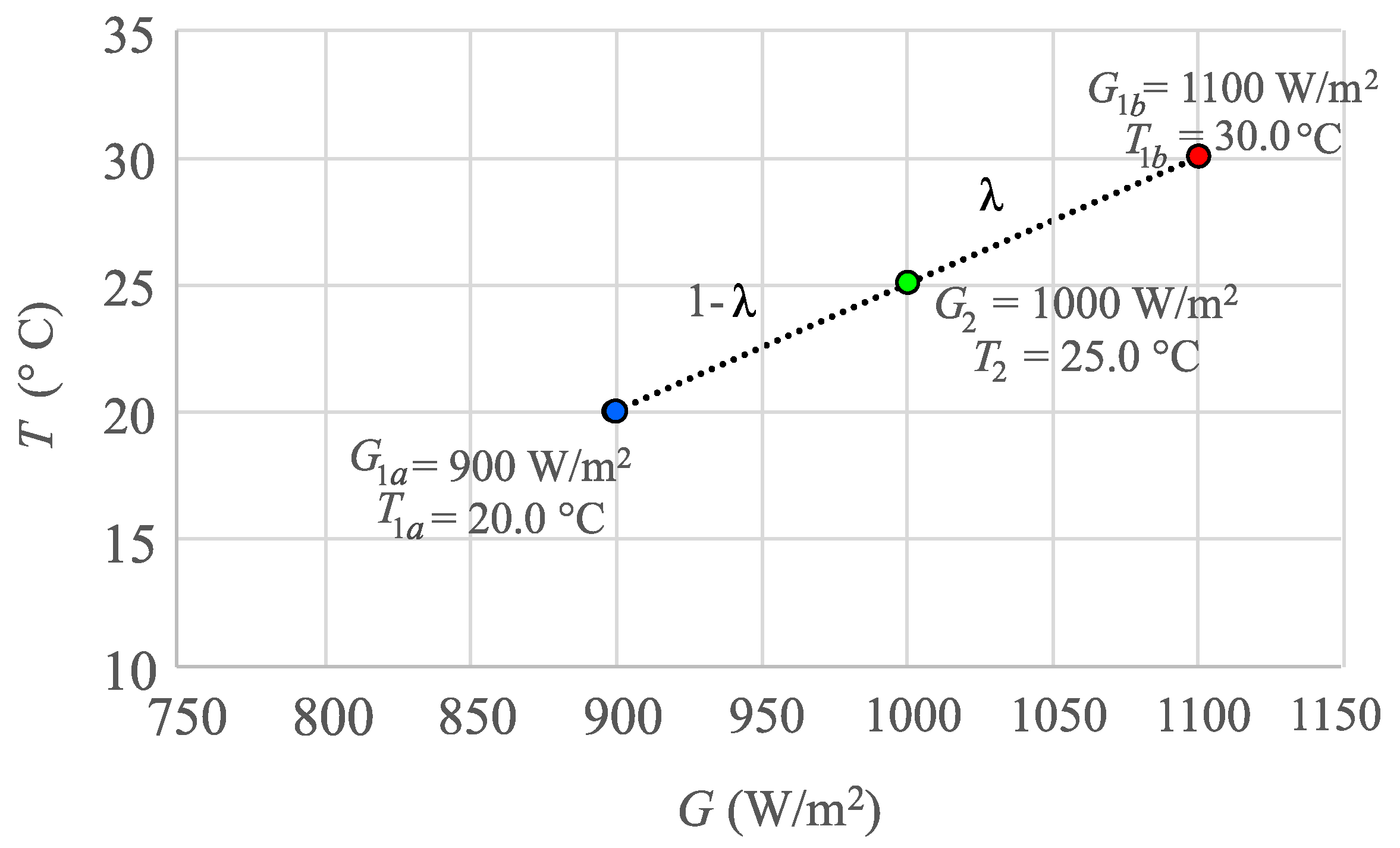
On the one hand, it is necessary to perform the interpolation in the temperature vs. irradiance space, as can be seen in Figure 4. Given the point $(G_{1a},T_{1a})$, representing the operating conditions of the Curve 1a, and the point $(G_{1b},T_{1b})$, representing the operating conditions of the Curve 1b, it is possible to connect both points with a straight line (Equation (283)) in such a way that any point $(G_2,T_2)$ belonging to this line can be expressed as a linear combination of both initial points:

$$(G_2,T_2)=(1-\lambda )·(G_{1a},T_{1a})+\lambda ·(G_{1b}-G_{1a})$$

(283)

where $\lambda$ is the weight to determine depending on both the initial conditions and the target conditions.

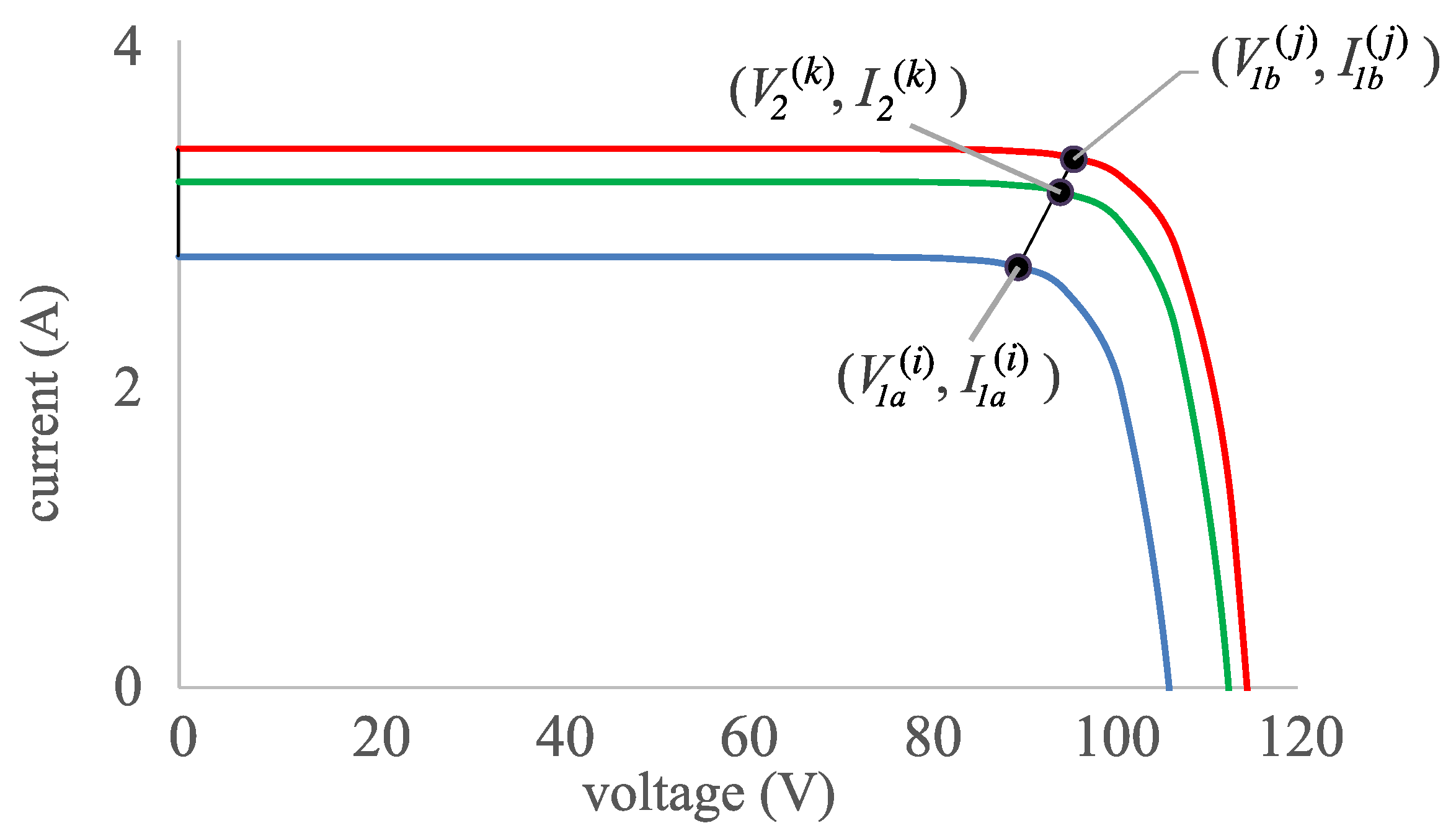
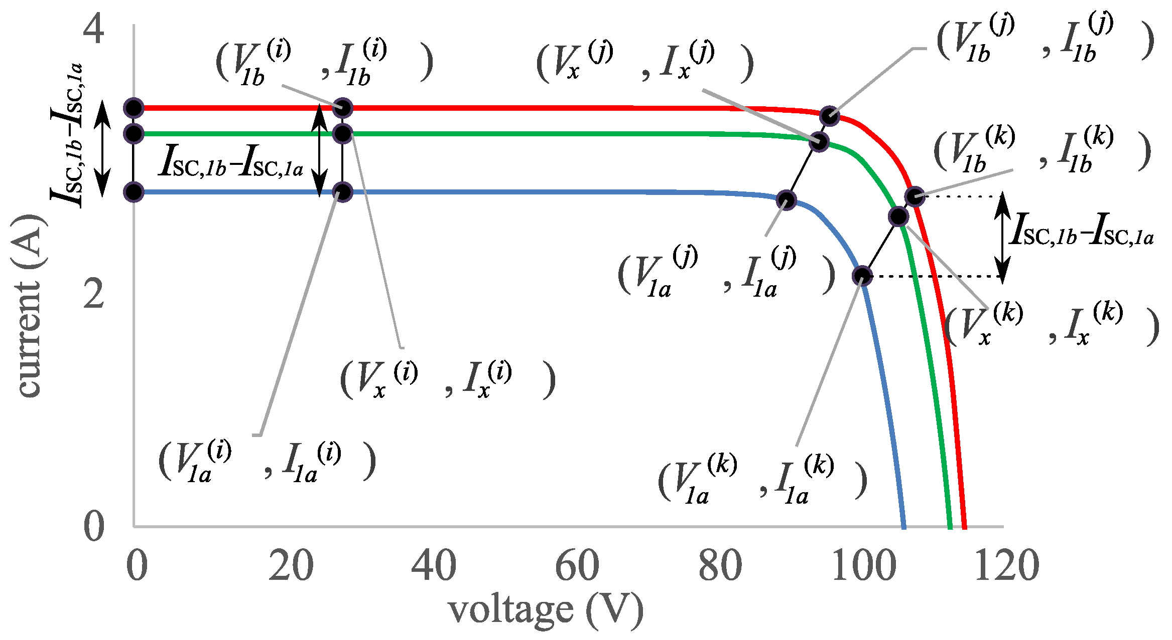
Once the value of the weight $\lambda$ is known, we can move on to reproducing a similar interpolation in the current versus voltage space (I–V plane). As can be seen in Figure 5, given a discrete point $\left(V_{1a}^{\left(i\right)},I_{1a}^{\left(i\right)}\right)$ (the i-th point belonging to Curve 1a) and another point $\left(V_{1b}^{\left(j\right)},I_{1b}^{\left(j\right)}\right)$ (the j-th point belonging to Curve 1b), it is possible to obtain a new point, supposed to belong to the final Curve 2 (its j-th point), which can be expressed as a linear combination of the previous points using exactly the same weight $\lambda$ as determined in the previous step (Equations (284) and (285)):

$$\begin{array}{c}{V}_2^{\left(k\right)}=(1-\lambda )·V_{1a}^{\left(i\right)}+\lambda ·V_{1b}^{\left(j\right)}\end{array}$$

(284)

$$\begin{array}{c}{I}_2^{\left(k\right)}=(1-\lambda )·I_{1a}^{\left(i\right)}+\lambda ·I_{1b}^{\left(j\right)}\end{array}$$

(285)

There are a pair problems that must be addressed. First, this procedure can be only used if the target conditions $(G_2,T_2)$ are able to be expressed as a linear combination of the operating conditions of both initial curves. Therefore, the applicability of this approach is very limited. In addition, from a practical point of view, care must be taken when selecting the pair of I–V points to be interpolated (one from Curve 1a and another one from Curve 1b). For each point of Curve 1a, which we can note as $(V_{1a}^{\left(i\right)},I_{1a}^{\left(i\right)})$, its is necessary to select a partner for Curve 1b, let this be $(V_{1b}^{\left(j\right)},I_{1b}^{\left(j\right)})$, but this selection is not trivial. We can select both points in such a way that (Equation (286)) is satisfied [3,76]:

$$I_{1b}^{\left(j\right)}-I_{1a}^{\left(i\right)}\simeq I_{\mathrm{SC}1\mathit{b}}-I_{\mathrm{SC}1\mathit{a}}$$

(286)

H02:

Bilinear Interpolation

Based on the previous approach H01, Marion et al. [7] presented an improved procedure of interpolation that takes as input four I–V curves, to perform a sort of bilinear interpolation. There are two different irradiance levels ($G_{high}$ and $G_{low}$) and two different temperature levels ($T_{high}$ and $T_{low}$), in such a way that each initial curve refers to the following operating conditions:

• Curve 1a: $\left\{V_{1a}^{\left(j\right)},I_{1a}^{\left(j\right)}\right\}$, where $j=1,\dots ,r_{1a}$, measured at an irradiance $G_{1a}=G_{low}$ and a cell temperature $T_{1a}=T_{low}$.
• Curve 1b: $\left\{V_{1b}^{\left(j\right)},I_{1b}^{\left(j\right)}\right\}$, where $j=1,\dots ,r_{1b}$, measured at an irradiance $G_{1b}=G_{high}$ and a cell temperature $T_{1b}=T_{low}$.
• Curve 1c: $\left\{V_{1c}^{\left(j\right)},I_{1c}^{\left(j\right)}\right\}$, where $j=1,\dots ,r_{1c}$, measured at an irradiance $G_{1c}=G_{low}$ and a cell temperature $T_{1c}=T_{high}$.
• Curve 1d: $\left\{V_{1d}^{\left(j\right)},I_{1d}^{\left(j\right)}\right\}$, where $j=1,\dots ,r_{1d}$, measured at an irradiance $G_{1d}=G_{high}$ and a cell temperature $T_{1d}=T_{high}$.

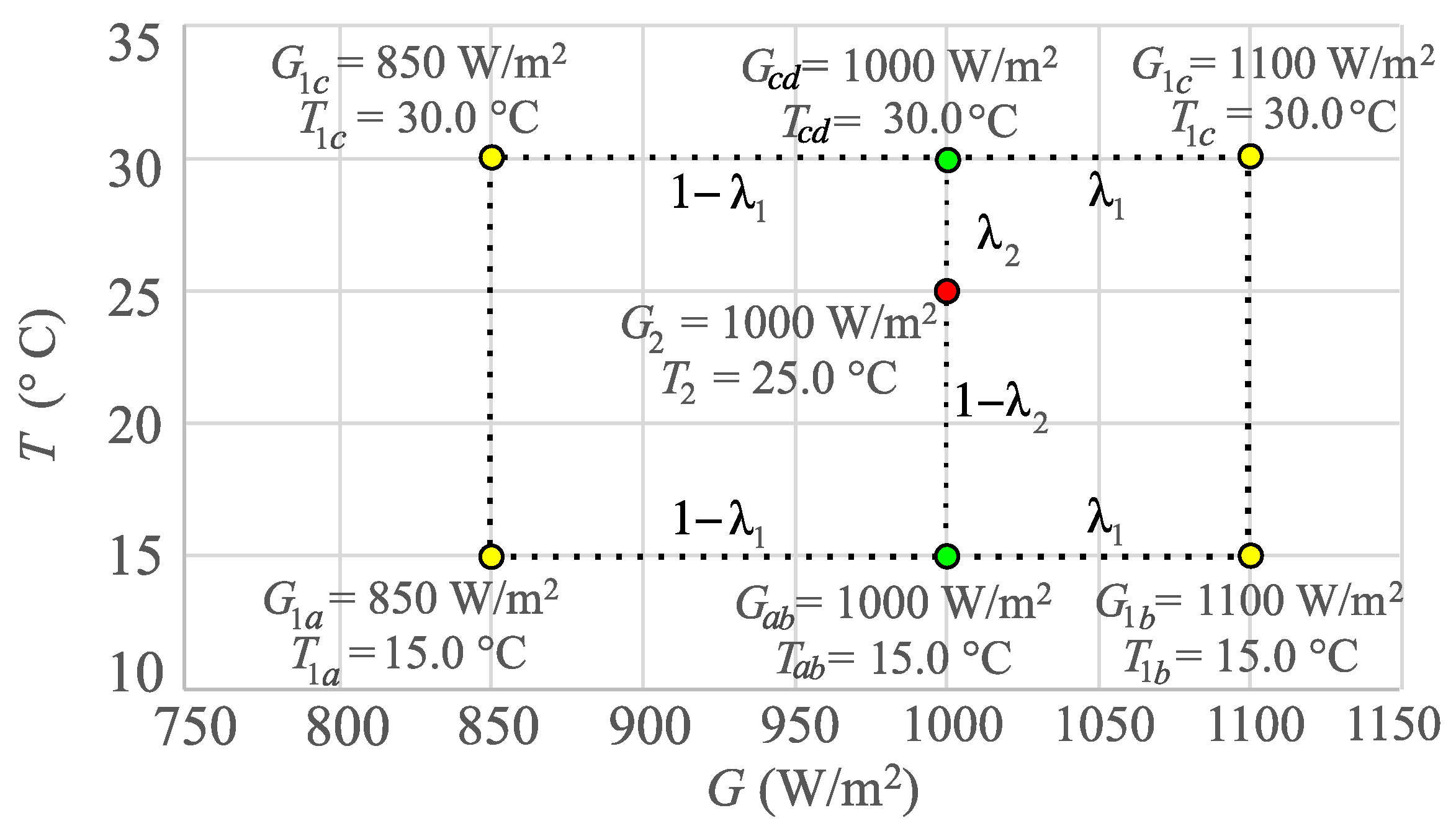
As can be seen in Figure 6, the points of the G/T plane representing these four I–V curve points are arranged on a square, and depending on how the are combined, it is possible to obtain through interpolation the corresponding I–V curve under any target conditions $(G_2,T_2)$. The following steps should be performed:

(a)

First, it is possible to perform a linear interpolation of Curve 1a and Curve 1b to create an auxiliary curve Curve ab, referring to $(G_2,T_{low})$. Let ${\lambda }_1$ be the weight used to perform the linear interpolation.

(b)

Then, it is also possible to perform a second linear interpolation of Curve 1c and Curve 1d to create a second auxiliary curve Curve cd, referring to $(G_2,T_{high})$. The weight used to perform the linear interpolation will be exactly ${\lambda }_1$, the same as used for the previous interpolation.

(c)

Finally, Curve ab and Curve cd are used as inputs when performing a final linear interpolation to generate Curve 2, referring to $(G_2,T_2)$. The weight used to perform the linear interpolation can be noted as ${\lambda }_2$.

The main drawback of this procedure is the task of achieving four I–V curves arranged as described in Figure 6, especially if the measurements are taken outdoors.

H03:

IEC 60891 procedure 3

Procedure 3 described in IEC 60891:2021 [3] has two possible versions: one that uses four I–V curves as input, but also a simplified variant in which only three I–V curves are required:

• Curve 1a: $\left\{V_{1a}^{\left(j\right)},I_{1a}^{\left(j\right)}\right\}$, where $j=1,\dots ,r_{1a}$, measured at an irradiance $G_{1a}$ and a cell temperature $T_{1a}$.
• Curve 1b: $\left\{V_{1b}^{\left(j\right)},I_{1b}^{\left(j\right)}\right\}$, where $j=1,\dots ,r_{1b}$, measured at an irradiance $G_{1b}$ and a cell temperature $T_{1b}$.
• Curve 1c: $\left\{V_{1c}^{\left(j\right)},I_{1c}^{\left(j\right)}\right\}$, where $j=1,\dots ,r_{1c}$, measured at an irradiance $G_{1c}$ and a cell temperature $T_{1c}$.

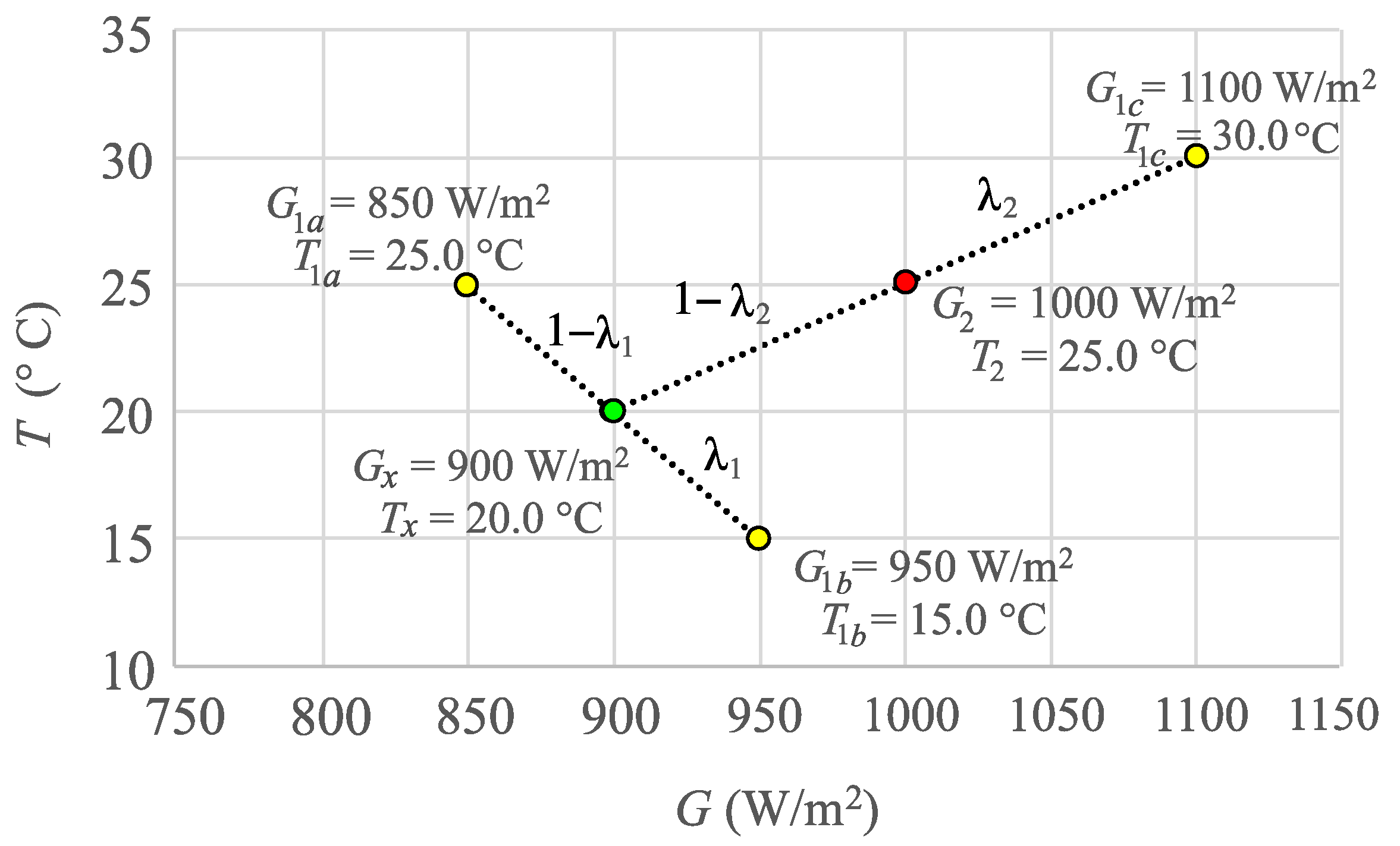
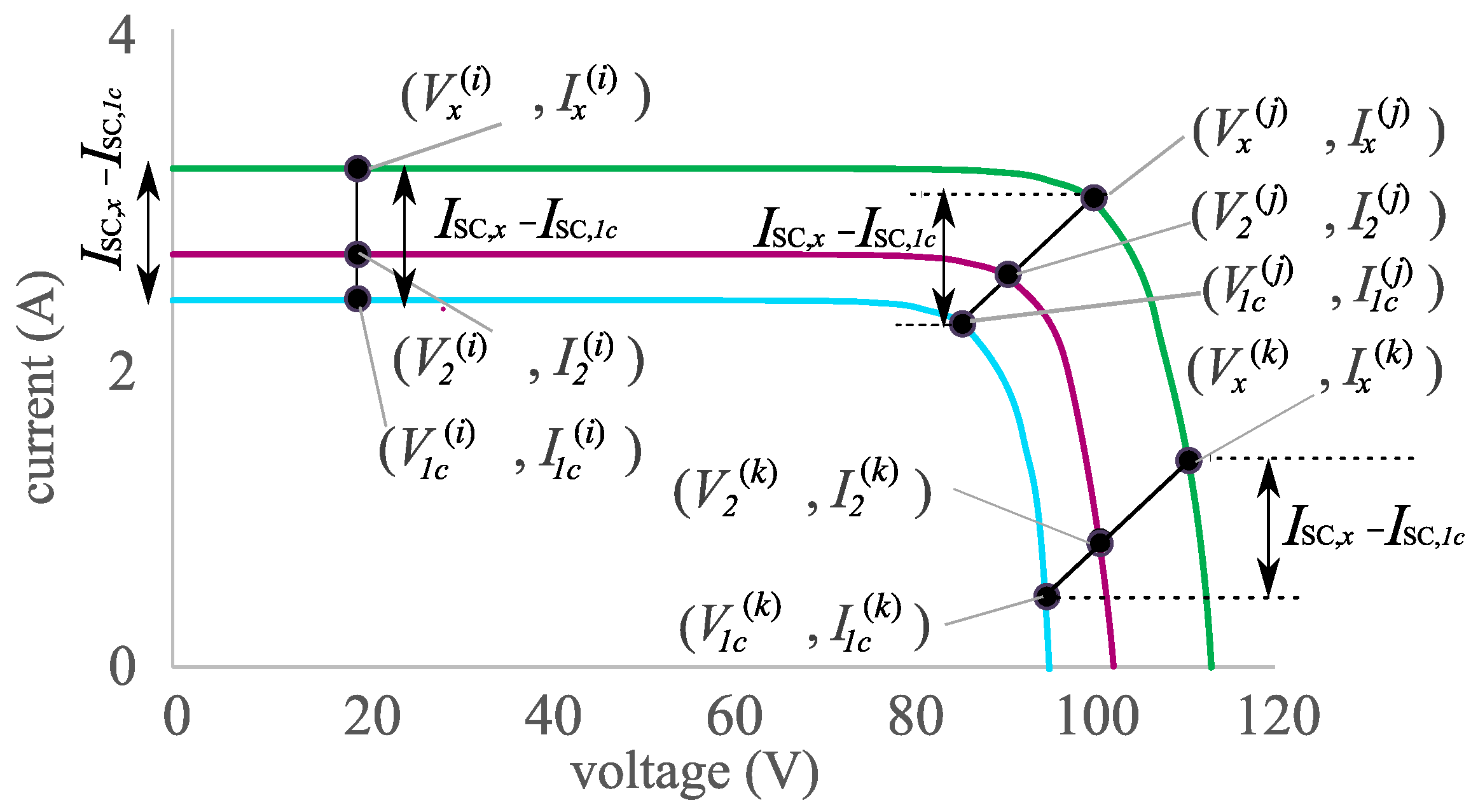
The advantage of this interpolation method with respect to the previous ones is that the I–V curves are not required to be arranged in any specific way. The operating conditions $(G_i,T_i)$ of these curves can be arranged on the G/T plane as any triangle (see Figure 7), in such a way that the I–V curve referring to any target conditions $(G_2,T_2)$ inside this triangle can be obtained through interpolation (extrapolation if the point is outside the triangle). The objective is to estimate a target curve $\left\{V_2^{\left(j\right)},I_2^{\left(j\right)}\right\}$ referring to $(G_2,T_2)$. This can be achieved by taking advantage of a auxiliary I–V curve $\left\{V_x^{\left(j\right)},I_x^{\left(j\right)}\right\}$, referring to the intermediate conditions $(G_x,T_x)$.This auxiliary Curve x is built from Curve 1a and Curve 1b using linear interpolation. In a second step, Curve 1c and Curve x are also used as input for a second interpolation to build the final target Curve 2.

First, it is necessary to perform the interpolation in the G/T space, as can be seen in Figure 7. Once the required weights ${\lambda }_1$ and ${\lambda }_2$ have been determined, it is possible to use those values to finish the interpolation in the I–V plane. The conditions $(G_x,T_x)$ are generated using a linear combination of $(G_{1a},T_{1a})$ and $(T_{1b},T_{1b})$ (see Equations (287) and (288)), with ${\lambda }_1$ the weight to estimate. The final conditions $(G_2,T_2)$ come from the interpolation of $(G_{1c},T_{1c})$ and $(G_x,T_x)$ by means of the other weight ${\lambda }_2$ (see Equations (289) and (290)). The values of the weights can be determined by solving a system of equations, whose unknowns are $G_x$, $T_x$, ${\lambda }_1$ and ${\lambda }_2$:

$$\begin{array}{c}{G}_x=(1-{\lambda }_1)·G_{1a}+{\lambda }_1·G_{1b}\end{array}$$

(287)

$$\begin{array}{c}{T}_x=(1-{\lambda }_1)·T_{1a}+{\lambda }_1·T_{1b}\end{array}$$

(288)

$$\begin{array}{c}{G}_2=(1-{\lambda }_2)·G_x+{\lambda }_2·G_{1c}\end{array}$$

(289)

$$\begin{array}{c}{T}_2=(1-{\lambda }_2)·T_x+{\lambda }_2·T_{1c}\end{array}$$

(290)

It is necessary to select, for each pair $\left(V_{1a}^{\left(j\right)},I_{1a}^{\left(j\right)}\right)$ in Curve 1a, its counterpart $\left(V_{1b}^{\left(j\right)},I_{1b}^{\left(j\right)}\right)$ of Curve 1b, verifying $I_{1b}^{\left(j\right)}-I_{1a}^{\left(j\right)}=\Delta I_1$ (where $\Delta I_1=I_{\mathrm{SC},1b}-I_{\mathrm{SC},1a}$). Then, from both pairs, a new pair $\left(V_x^{\left(j\right)},I_x^{\left(j\right)}\right)$ of the new Curve x is generated using (Equations (291) and (292)). Similarly, defining $\Delta I_2=I_{\mathrm{SC},x}-I_{\mathrm{SC},1c}$, using a point from Curve 1c and its counterpart in Curve x (satisfying $I_x^{\left(j\right)}-I_{1c}^{\left(j\right)}=\Delta I_2$), the pair $\left(V_2^{\left(j\right)},I_2^{\left(j\right)}\right)$ of Curve 2 can be obtained using (Equations (293) and (294)). This process is sketched in Figure 8 and Figure 9.

$$\begin{array}{c}{V}_x^{\left(j\right)}=(1-{\lambda }_1)·V_{1a}^{\left(j\right)}+{\lambda }_1·V_{1b}^{\left(j\right)}\end{array}$$

(291)

$$\begin{array}{c}{I}_x^{\left(j\right)}=(1-{\lambda }_1)·I_{1a}^{\left(j\right)}+{\lambda }_1·I_{1b}^{\left(j\right)}\end{array}$$

(292)

$$\begin{array}{c}{V}_2^{\left(j\right)}=(1-{\lambda }_2)·V_x^{\left(j\right)}+{\lambda }_2·V_{1c}^{\left(j\right)}\end{array}$$

(293)

$$\begin{array}{c}{I}_2^{\left(j\right)}=(1-{\lambda }_2)·I_x^{\left(j\right)}+{\lambda }_2·I_{1c}^{\left(j\right)}\end{array}$$

(294)

This method has several drawbacks that must be clearly highlighted. First, for its application, it is not enough to use a unique I–V curve as input, because we need to measure three of them. Moreover, the points $(G_{1i},T_{1i})$ associated with these three curves must be arranged in the irradiance/temperature plane on a triangular shape, in such a way the point $(G_2,T_2)$ representing the target conditions should be inside this triangle. Therefore, in order to test this method, it is necessary to find measurements of I–V curves verifying that requirement.

A second drawback of this methodology is the fact that during the interpolation of two initial I–V curves, for each iteration, it is necessary to identify different pairs of points to be interpolated (one from the first I–V curve and another from the second input I–V curve). This step is not clearly explained in the standard IEC 60891:2021, and depending on how the points are distributed along both I–V curves, a deformed I–V curve could be obtained, so a visual inspection of the result may be necessary.

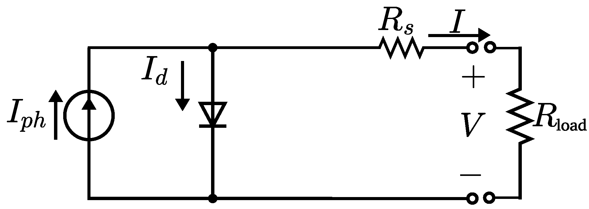2. Methodology

2.1. Description of PV Modules and Measurement Facilities

All the methods under study in this work were tested for comparative purposes using two commercial photovoltaic modules with crystalline silicon technologies. The first module from Isofoton, model ISF-145, has 36 cells connected in series, single crystalline silicon (sc-Si) cells, and a side of 156 mm. A second module from Kyocera, model KD140GH-2PU, also composed off 36 cells of 156 mm size, was also tested. For both modules,

Table 3. Nominal, experimental, and technology-dependent values of the required parameters.

		ISF-145 (sc–Si)		KD140GH-2PU (mc–Si)
		Nominal	Actual	Nominal	Actual
$I_{\mathrm{SC},\mathrm{STC}}$	[A]	8.55	8.545	8.68	8.545
$V_{\mathrm{OC},\mathrm{STC}}$	[V]	22.4	22.05	22.1	21.84
$P_{\mathrm{M},\mathrm{STC}}$	[W]	145	142.3	140	137.4
$I_{\mathrm{M},\mathrm{STC}}$	[A]	8.00	7.994	7.91	7.887
$V_{\mathrm{M},\mathrm{STC}}$	[V]	18.1	17.80	17.7	17.42
$\alpha$	[A/K]	+0.00359	+0.0033	+0.00052	+0.0057
${\alpha }_r$	[1/K]	+0.00042	+0.00039	+0.0006	+0.00067
$\beta$	[V/K]	−0.0724	−0.0747	−0.0796	−0.062
${\beta }_r$	[1/K]	−0.00323	−0.0034	−0.0036	−0.0028
$\gamma$	[W/K]	−0.673	−0.665	−0.644	−0.52
${\gamma }_r$	[1/K]	−0.00464	−0.00467	−0.0046	−0.0038
$R_{s,\mathrm{STC}}$	[$\Omega$]		0.147		0.170
$\kappa$	[$\Omega$/K]		+0.00048		+0.00040
$B_S$	[1/K]		0.0031		0.0023
m	[−]		1.210		1.253
$\delta$	[−]		0.049		0.068
${\delta }_1$	[−]		0.037		0.032
${\delta }_2$	[−]		0.069		0.172
$\xi$	[−]		0.9493		0.9290
$\chi$	[−]		1.0713		0.9707
$E_{g0K}$	[eV]	1.1557	[79]	1.1557	[79]
${\rho }_A$	[eV/K]	7.021×$\times {10}^{-4}$	[79]	7.021$\times {10}^{-4}$	[79]
${\rho }_B$	[K]	1108	[79]	1108	[79]
$\eta$	[−]	540.7	[18]	219.7	[18]
$\lambda$	[−]	0.9	[18]	0.75	[18]
$\mathcal{R}$	[−]	4	[52]	4	[52]
$\nu$	[−]	5.5	[52]	5.5	[52]

shows the information provided by the manufacturer in their data, in addition to the values of other parameters required by the methods and estimated by ourselves using measurements under outdoor conditions. The modules were measured on the terrace of the Laboratory of Photovoltaic Systems of Malaga University (Malaga, Spain). Both specimens were installed on an open-rack structure and connected to an experimental I–V curve tracer composed of different laboratory instruments controlled by a personal computer. A scheme of the measurement system can be seen in Figure 10. More details about these systems and the uncertainty of the measurements can be found in Piliougine et al. [85].

As we wanted to simulate as much as possible the operating conditions of a real solar plant, we decided to take the measurements under outdoor conditions, so we installed both devices under test on a open-rack structure placed on the roof of the laboratory, in such a way that the source of light for these experiments was the actual sun. The received irradiance was measured using a pyranometer, but also using a calibrated PV cell, to have a fast sensor to reject the curves acquired under non-stable conditions.

For a single unencapsulated PV cell under laboratory conditions (using a thermal chamber and an artificial light source), it is possible to use a temperature sensor, assuming its reading as the actual cell temperature. However, that scenario was not the case for the experiments carried out in this work. We decided to test the different methods under realistic outdoor conditions using commercial PV modules (with many cells connected in series/parallel between different encapsulating layers). In these cases, there is always a gradient between the internal cell temperature and the temperature measured using a sensor installed on the back external surface [83], in such a way that it is practically impossible to make a direct measurement of the actual internal temperature.

For the reason explained above, it is only possible to approximate the value of the actual internal temperature $T_c$ of a device using a model; for example, using the expression proposed by King et al. [83] (Equation (295)), which uses as input the back-surface temperature $T_b$ and the irradiance reading G. Therefore, for the experiments conducted in this work, we estimated the internal temperature $T_c$ from the external value $T_b$ provided by the temperature sensor, which was lower. This difference $\Delta \mathrm{T}$ is around $3$ °C for a typical PV module with glass/cell/tedlar mounted on a open-rack structure, which was exactly our case. Therefore, a constant $\Delta \mathrm{T}=3$ °C was assumed to be a generic value representing the difference between the internal temperature $T_c$ and the back-surface temperature $T_b$ when the incident irradiance was 1000 W/m${}^2$ (${\mathrm{G}}_{\mathrm{STC}}$). However, as can be seen in the proposed expression, if the irradiance is higher than ${\mathrm{G}}_{\mathrm{STC}}$, this difference (internal/external) of $3$ °C is scaled up to be higher.

$$T_c=T_b+{\displaystyle \frac{G}{{\mathrm{G}}_{\mathrm{STC}}}}·\Delta \mathrm{T}$$

(295)

Under outdoor conditions, it is not realistic to assume a free-mismatch scenario in terms of cell temperature, in such a way that each cell of the device operates under its own temperature within a range. Although this fact leads us to certain degree of uncertainty if any of these methods are applied under a PV module/array, this issue was assumed in the standard IEC 60891:2021 [3] and in the standard IEC 60904–1 [94], because in both of them, it is recommended to install four temperature sensors on the back surface of the device under study, even providing a scheme proposing the places to attach such temperature sensors and averaging their readings to obtain $T_b$.

Therefore, in this work, the back-side temperature $T_b$ was computed as the mean value of the readings from four temperature sensors RTD Pt100, placed as indicated in the previous standards. The main reason for using Pt100 to measure the back-side temperature was that our measurement system had a module for reading this type of sensor using a 4-wire configuration. On the one hand, the experimental (actual) values of the temperature coefficients in Table 3 ($\alpha$, $\beta$, $\gamma$,…) were estimated according to previous literature [76,77]: a sequence of I–V curves were measured under increasing cell temperature within a very narrow irradiance interval ($G=1000\pm 20$ W/m${}^2$) and in such a way that the slopes of the respective regression lines were the required temperature coefficients. On the other hand, to estimate other parameters, a curve-fitting procedure was applied to each I–V curve using SDM as the underlying model.

2.2. Description of the Test Sets and Error Metrics

The I–V curve curve tracer takes a measurement every 5 min over several days under outdoor conditions, and after this period, three different groups of curves were selected for creating the different test sets, with different mean values and standard deviations for the irradiance and the cell temperature. The different methods were compared by means several test sets, noted as TEST1(a|b), TEST2(a|b), and TEST3(a|b), with an increasing difficulty (a refers to module ISF-145 and b refers to module KD140GH-2PU). Each test set included $\mathcal{N}=30$ experimental I–V curves measured under different conditions, which had to be corrected to the measurement conditions of a reference I–V curve. Then, the corrected curves were compared to the reference curve according to the following error metrics:

• MAPE of the short-circuit current $I_{\mathrm{SC}}$.
• MAPE of the open-circuit voltage $I_{\mathrm{OC}}$.
• MAPE of the maximum power $P_{\mathrm{M}}$.
• MAPE of the current at the maximum power point $I_{\mathrm{M}}$.
• MAPE of the voltage at the maximum power point $V_{\mathrm{M}}$.
• Average value of the relative global curve error.

where MAPE stands for mean absolute percentage error, estimated using (Equation (296)), assuming that $y_i$ is each electrical parameter of the reference curve and ${\widehat{y}}_i$ is the same electrical parameter of each translated curve:

$$\mathit{MAPE}=100\%·\frac{1}{\mathcal{N}}·\sum _{i=1}^{\mathcal{N}}\left|{\displaystyle \frac{y_i-{\widehat{y}}_i}{y_i}}\right|$$

(296)

and the curve error [95] is a measurement of the similarity between each corrected and measured I–V curve based on the area between them (see Figure 11). For each cross-point between both curves, a partial area $A_i$ was estimated using numerical integration. Then, all the partial areas were summed (Equation (297)), and finally, the value was divided by the area $A_0$ enclosed between the measured curve and the first quadrant.

$$\mathit{curveError}=100\%·\frac{1}{A_0}·\sum _i{A}_i$$

(297)

It should be taken into account that, when using the module ISF-145 the irradiance $G_2=1007$ W/m${}^2$ of the reference curve and its temperature $T_2=45.1$ °C were used as target conditions for all the test sets, whereas for the module KD140GH-2PU, the target conditions were $G_2=974$ W/m${}^2$ and $T_2=25.2$ °C.

Table 4. Minimum, maximum, mean, and standard deviation of the test sets used with module ISF-145.

Set	$min\left(\mathit{G}\right)$	$max\left(\mathit{G}\right)$	$\mathit{\mu }\left(\mathit{G}\right)$	$\mathit{\sigma }\left(\mathit{G}\right)$	$min\left(\mathit{T}\right)$	$max\left(\mathit{T}\right)$	$\mathit{\mu }\left(\mathit{T}\right)$	$\mathit{\sigma }\left(\mathit{T}\right)$
	W/m${}^{\mathbf{2}}$	W/m${}^{\mathbf{2}}$	W/m${}^{\mathbf{2}}$	W/m${}^{\mathbf{2}}$	°C	°C	°C	°C
TEST1a	1002	1019	1010	6	42.0	47.9	44.8	1.9
TEST2a	980	1022	991	16	29.8	55.5	38.0	9.3
TEST3a	764	849	834	19	29.3	54.9	51.3	6.2

and

Table 5. Minimum, maximum, mean, and standard deviation of the test sets used with module KD140GH-2PU.

Set	$min\left(\mathit{G}\right)$	$max\left(\mathit{G}\right)$	$\mathit{\mu }\left(\mathit{G}\right)$	$\mathit{\sigma }\left(\mathit{G}\right)$	$min\left(\mathit{T}\right)$	$max\left(\mathit{T}\right)$	$\mathit{\mu }\left(\mathit{T}\right)$	$\mathit{\sigma }\left(\mathit{T}\right)$
	W/m${}^{\mathbf{2}}$	W/m${}^{\mathbf{2}}$	W/m${}^{\mathbf{2}}$	W/m${}^{\mathbf{2}}$	°C	°C	°C	°C
TEST1b	973	985	977	3	20.0	29.7	25.0	3.1
TEST2b	957	1005	986	12	21.7	47.6	36.1	8.6
TEST3b	754	847	802	26	12.5	37.0	26.4	11.2

describe the different test sets used for the modules ISF-145 and KD140GH-2PU, respectively, providing their minimum, maximum, mean, and standard deviation. As can be seen, TEST1a and TEST1b implied very small translations in terms of irradiance and cell temperature, so the different error metrics also gave small values. On the contrary, in TEST2a and TEST2b, there was a higher dispersion of the measurement conditions, mainly because the temperature range was larger. In the case of TEST3a and TEST3b, the difficulty was even greater, because the irradiance jump between the initial and target conditions was huge.

In order to test the interpolation methods (type H), it was required to use more than one initial I–V curve. Therefore, it was not possible to directly use the test sets described above. In the case of the method H03, instead of correcting each I–V curve individually, we took several combinations of curves (within the respective ranges specified in Table 4 or Table 5) arranged on a triangular shape, as specified in Figure 7. However, to apply the method H01, it was necessary to find pairs of initial I–V curves in such a way that the target condition could be expressed as a linear combination of the conditions of those two initial curves. Another issue arises if method H02 has to be applied, because we need to search several combinations of four I–V curves belonging to the test set whose measurement conditions are arranged in a similar way to the yellow dots in Figure 6. As the reader can imagine, under outdoor conditions (which was our case), it is practically impossible to find curves arranged on a straight line (for H01) or on a rectangular shape (for H2). Therefore, in this comparative review, methods H01 and H02 were excluded from the experimental comparison, due to the difficulty of their application.

3. Results

This section aims to analyze the results of the different methods (summarized in Table 1) over the outdoor experimental I–V curves measured from the modules ISF-145 and KD140GH-2PU. As for each module we built three test sets, there are a total of six tables (from

Table 6. Error metrics of all methods for TEST1a on ISF-145.

		MAPE (%)					Curve
Id.  —  Abbr.		${\mathit{I}}_{\mathrm{SC}}$	${\mathit{V}}_{\mathrm{OC}}$	${\mathit{P}}_{\mathrm{M}}$	${\mathit{I}}_{\mathrm{M}}$	${\mathit{V}}_{\mathrm{M}}$	Error
A01	BASIC	0.16	0.20	0.16	0.18	0.13	0.68
A02	RBACH	0.16	0.23	0.15	0.18	0.16	0.76
A03	CASTAÑER	0.16	0.16	0.17	0.18	0.11	0.57
A04	REDDY	0.16	0.15	0.19	0.18	0.12	0.60
A05	ANDERSON	0.16	0.15	0.19	0.18	0.12	0.58
	†			0.19
A06	SMITH	0.16	0.18	0.18	0.18	0.13	0.51
	†			0.18
A07	CARRILLO	0.16	0.17	0.16	0.18	0.11	0.66
A08	DIA	0.16	0.20	0.16	0.18	0.13	0.69
A09	ZHOU	0.14	0.15	0.18	0.16	0.12	0.53
A10	BATZELIS	0.16	0.15	0.19	0.18	0.12	0.57
	†			0.16	0.17	0.23
B01	BLAESSER	0.16	0.17	0.16	0.18	0.13	0.71
B02	ALONSO	0.16	0.17	0.15	0.17	0.19	0.57
B03	JRC	0.16	0.15	0.14	0.17	0.17	0.47
B04	IEC-P1	0.16	0.17	0.16	0.17	0.21	0.50
B05	IEC-P1(b)	0.16	0.16	0.14	0.17	0.19	0.46
B06	IEC-P2	0.16	0.15	0.15	0.17	0.19	0.52
B07	IEC-P2(b)	0.16	0.15	0.15	0.17	0.18	0.53
B08	IEC-P2(c)	0.16	0.16	0.15	0.17	0.20	0.48
B09	IEC-P4	0.17	0.16	0.21	0.18	0.23	0.63
B10	IEC-P4(b)	0.17	0.23	0.32	0.18	0.30	0.65
C01	ISDM	0.70	0.35	3.29	2.81	0.50	1.22
C02	SSDM	0.24	0.20	0.28	0.15	0.23	0.92
C03	SDM	0.15	0.20	0.28	0.19	0.23	0.71
C04	SDM(b)	0.15	0.20	0.28	0.19	0.24	0.70
C05	RUSCHELL	0.15	0.20	0.29	0.21	0.23	0.62
C06	PVSYST	0.15	0.20	0.29	0.21	0.23	0.65
C07	WALKER	0.15	0.19	0.26	0.19	0.23	0.60
C08	LAURINO	0.15	0.19	0.29	0.19	0.25	0.71
C09	DING	0.15	0.19	0.29	0.19	0.25	0.71
C10	COTFAS	0.15	0.20	0.31	0.19	0.25	0.74
C11	SSDM(b) *	0.22	0.20	0.27	0.13	0.23	0.89
C12	SDM *	0.22	0.29	0.33	0.14	0.38	0.86
C13	PVSYST *	0.13	0.20	0.28	0.19	0.23	0.79
C14	WALKER *	0.13	0.19	0.27	0.19	0.22	0.68
C15	LAURINO *	0.13	0.19	0.28	0.17	0.25	0.66
D01	SDDM	0.16	0.20	0.33	0.46	0.30	0.61
D02	DDM5p	0.16	0.20	0.33	0.46	0.30	0.61
D03	DDM6p	0.15	0.23	0.31	0.19	0.26	0.87
D04	DDM7p	0.16	0.19	0.27	0.21	0.23	0.60
D05	SDDM *	0.14	0.20	0.32	0.45	0.30	0.56
D06	DDM5p *	0.14	0.20	0.32	0.45	0.30	0.56
D07	DDM6p *	0.19	0.21	0.31	0.22	0.24	0.69
D08	DDM7p *	0.15	0.19	0.27	0.21	0.23	0.74
E01	LOBRANO	0.23	0.20	0.52	0.15	0.45	0.57
E02	SERA	0.15	0.18	0.27	0.39	0.29	0.59
E03	ORIOLI	0.17	0.14	0.16	0.99	0.96	0.77
E04	DeSOTO	0.22	0.28	0.96	0.73	1.58	1.34
E05	TOLEDO	0.17	0.19	0.37	0.19	0.25	0.71
E06	XIAO	0.16	0.18	0.26	0.17	0.25	0.80
E07	LoBRANO *	0.24	0.20	0.51	0.13	0.45	0.63
E08	SERA *	0.13	0.19	0.26	0.37	0.29	0.52
E09	ORIOLI *	0.14	0.14	0.17	0.97	0.96	0.73
E10	DeSOTO *	0.20	0.28	0.96	0.72	1.58	1.25
E11	TOLEDO *	0.14	0.19	0.36	0.17	0.25	0.78
E12	XIAO *	0.14	0.18	0.26	0.15	0.25	0.91
F01	SALOUX	0.16	0.14	0.19	1.86	1.99	1.32
F02	PHANG	0.17	0.19	0.25	0.14	0.24	1.09
F03	CUBAS(a)	0.17	0.38	0.49	0.18	0.44	0.62
F04	CUBAS(b)	0.37	0.10	0.31	0.36	0.15	1.42
F05	CUBAS(c)	0.17	0.37	0.49	0.18	0.43	0.70
F06	KHAN	0.17	0.19	0.36	0.20	0.25	0.71
F07	PETRONE	0.25	0.24	0.25	0.63	0.57	0.98
F08	SPRATIO	0.14	0.20	0.25	0.15	0.25	0.82
F09	BAI	0.15	0.19	0.33	0.16	0.26	0.83
F10	CRISTALDI	0.16	0.15	0.17	0.16	0.19	0.35
F11	SERA(b)	0.14	0.42	0.54	0.16	0.48	0.80
F12	TOLEDO(b)	0.15	0.39	0.50	0.12	0.47	1.05
F13	BATZELIS(b)	0.16	0.20	0.27	0.49	0.73	1.20
F14	SALOUX *	0.14	0.14	0.21	1.84	2.00	1.31
F15	PHANG *	0.15	0.19	0.25	0.12	0.24	1.01
F16	CUBAS(a) *	0.15	0.38	0.49	0.16	0.44	0.79
F17	CUBAS(b) *	0.35	0.10	0.30	0.34	0.15	1.43
F18	CUBAS(c) *	0.15	0.37	0.48	0.16	0.43	0.84
F19	KHAN *	0.15	0.19	0.34	0.18	0.25	0.83
F20	PETRONE *	0.23	0.24	0.25	0.62	0.57	0.98
F21	SPRATIO *	0.14	0.20	0.25	0.15	0.25	0.82
F22	BAI *	0.15	0.19	0.33	0.16	0.26	0.83
F23	CRISTALDI *	0.14	0.15	0.17	0.14	0.19	0.32
F24	SERA(b) *	0.14	0.42	0.54	0.16	0.48	0.80
F25	TOLEDO(b) *	0.15	0.39	0.50	0.12	0.47	1.05
F26	BATZELIS(b) *	0.14	0.20	0.30	0.47	0.73	1.20
G01	VILLALVA	0.18	0.40	0.52	0.44	0.50	0.75
G02	BOUTANA	0.16	0.15	1.29	1.45	0.30	0.75
G03	CARRERO	0.16	0.18	0.22	0.16	0.25	0.82
G04	STORNELLI	0.16	0.19	0.27	0.51	0.44	0.64
G05	VILLALVA *	0.16	0.40	0.51	0.42	0.50	0.65
G06	BOUTANA *	0.14	0.15	1.28	1.44	0.30	0.73
G07	CARRERO *	0.14	0.19	0.24	0.14	0.26	0.76
G08	STORNELLI *	0.14	0.19	0.27	0.49	0.44	0.56
H03	IEC-P3	0.08	0.03	0.14	0.12	0.04	0.38

† Result obtained using direct formula instead of curve translation. * Equal to the original method using (Equation (88)) instead of (Equation (76)).

,

Table 7. Error metrics of all methods for TEST1b on KD140GH-2PU.

		MAPE (%)					Curve
Id.  —  Abbr.		${\mathit{I}}_{\mathrm{SC}}$	${\mathit{V}}_{\mathrm{OC}}$	${\mathit{P}}_{\mathrm{M}}$	${\mathit{I}}_{\mathrm{M}}$	${\mathit{V}}_{\mathrm{M}}$	Error
A01	BASIC	0.15	0.10	0.47	0.25	0.38	0.65
A02	RBACH	0.15	0.11	0.46	0.25	0.38	0.63
A03	CASTAÑER	0.15	0.10	0.47	0.25	0.39	0.68
A04	REDDY	0.15	0.09	0.47	0.25	0.38	0.63
A05	ANDERSON	0.15	0.09	0.47	0.25	0.38	0.66
	†			0.19
A06	SMITH	0.15	0.11	0.48	0.25	0.39	0.63
	†			0.18
A07	CARRILLO	0.15	0.10	0.47	0.25	0.38	0.71
A08	DIA	0.15	0.10	0.47	0.25	0.38	0.68
A09	ZHOU	0.13	0.06	0.35	0.23	0.25	0.49
A10	BATZELIS	0.15	0.10	0.47	0.25	0.39	0.69
	†			0.21	0.26	0.16
B01	BLAESSER	0.15	0.09	0.46	0.25	0.37	0.69
B02	ALONSO	0.14	0.09	0.29	0.26	0.25	0.45
B03	JRC	0.15	0.09	0.29	0.25	0.25	0.52
B04	IEC-P1	0.15	0.10	0.26	0.26	0.22	0.50
B05	IEC-P1(b)	0.15	0.10	0.30	0.26	0.26	0.52
B06	IEC-P2	0.15	0.09	0.26	0.25	0.21	0.50
B07	IEC-P2(b)	0.15	0.09	0.26	0.25	0.21	0.48
B08	IEC-P2(c)	0.15	0.10	0.26	0.25	0.22	0.44
B09	IEC-P4	0.15	0.10	0.25	0.26	0.13	0.61
B10	IEC-P4(b)	0.15	0.29	0.48	0.27	0.35	0.82
C01	ISDM	0.42	0.36	3.34	2.58	0.78	1.11
C02	SSDM	0.50	0.16	0.26	0.19	0.29	0.60
C03	SDM	0.17	0.15	0.25	0.13	0.15	0.73
C04	SDM(b)	0.17	0.15	0.25	0.13	0.15	0.80
C05	RUSCHELL	0.19	0.15	0.25	0.13	0.15	0.76
C06	PVSYST	0.19	0.15	0.26	0.14	0.15	0.61
C07	WALKER	0.17	0.13	0.23	0.13	0.13	0.68
C08	LAURINO	0.17	0.12	0.26	0.13	0.16	0.82
C09	DING	0.17	0.12	0.26	0.13	0.16	0.82
C10	COTFAS	0.17	0.15	0.30	0.13	0.20	1.18
C11	SSDM(b) *	0.48	0.16	0.25	0.19	0.29	0.67
C12	SDM *	0.47	0.26	0.42	0.10	0.40	0.75
C13	PVSYST *	0.19	0.15	0.24	0.12	0.15	0.70
C14	WALKER *	0.19	0.13	0.22	0.12	0.13	0.83
C15	LAURINO *	0.17	0.12	0.24	0.12	0.16	0.90
D01	SDDM	0.35	0.13	0.36	0.37	0.12	0.66
D02	DDM5p	0.19	0.13	0.35	0.44	0.13	0.56
D03	DDM6p	0.15	0.15	0.31	0.25	0.15	0.65
D04	DDM7p	0.15	0.13	0.27	0.23	0.12	0.55
D05	SDDM *	0.33	0.13	0.34	0.35	0.12	0.70
D06	DDM5p *	0.33	0.13	0.34	0.36	0.12	0.71
D07	DDM6p *	0.31	0.13	0.35	0.41	0.14	0.53
D08	DDM7p *	0.20	0.13	0.26	0.24	0.11	0.68
E01	LOBRANO	0.14	0.17	0.36	0.34	0.62	0.49
E02	SERA	0.14	0.13	0.26	0.29	0.12	0.63
E03	ORIOLI	0.17	0.10	0.19	0.34	0.26	0.66
E04	DeSOTO	0.35	0.22	1.24	1.21	1.56	1.50
E05	TOLEDO	0.21	0.15	0.36	0.29	0.15	0.81
E06	XIAO	0.15	0.13	0.29	0.26	0.14	0.60
E07	LoBRANO *	0.13	0.17	0.34	0.36	0.62	0.65
E08	SERA *	0.12	0.13	0.24	0.27	0.12	0.55
E09	ORIOLI *	0.15	0.10	0.18	0.32	0.26	0.62
E10	DeSOTO *	0.34	0.22	1.23	1.20	1.56	1.49
E11	TOLEDO *	0.19	0.15	0.35	0.27	0.15	0.76
E12	XIAO *	0.13	0.13	0.28	0.24	0.14	0.84
F01	SALOUX	0.15	0.10	0.12	1.57	1.52	1.45
F02	PHANG	0.17	0.16	0.29	0.21	0.32	0.64
F03	CUBAS(a)	0.17	0.77	1.00	0.29	0.84	1.22
F04	CUBAS(b)	0.34	0.13	0.38	0.46	0.13	1.32
F05	CUBAS(c)	0.20	0.55	0.71	0.33	0.59	1.01
F06	KHAN	0.17	0.17	0.76	0.26	0.60	0.60
F07	PETRONE	0.41	0.13	0.15	0.73	0.60	1.73
F08	SPRATIO	0.15	0.18	0.31	0.26	0.16	0.77
F09	BAI	0.17	0.17	0.97	0.33	0.65	0.65
F10	CRISTALDI	0.15	0.10	0.19	0.25	0.16	0.64
F11	SERA(b)	0.15	0.99	1.29	0.28	1.10	1.29
F12	TOLEDO(b)	0.17	0.68	0.90	0.20	0.75	1.05
F13	BATZELIS(b)	0.15	0.16	0.23	0.41	0.63	1.36
F14	SALOUX *	0.13	0.10	0.12	1.55	1.52	1.55
F15	PHANG *	0.16	0.16	0.27	0.21	0.32	0.70
F16	CUBAS(a) *	0.15	0.77	0.99	0.27	0.84	1.24
F17	CUBAS(b) *	0.32	0.13	0.36	0.44	0.13	1.24
F18	CUBAS(c) *	0.18	0.55	0.70	0.31	0.59	1.02
F19	KHAN *	0.15	0.17	0.74	0.25	0.60	0.70
F20	PETRONE *	0.39	0.13	0.14	0.72	0.60	1.63
F21	SPRATIO *	0.13	0.18	0.29	0.24	0.16	0.83
F22	BAI *	0.15	0.17	0.95	0.31	0.65	0.79
F23	CRISTALDI *	0.13	0.10	0.18	0.23	0.16	0.52
F24	SERA(b) *	0.13	0.99	1.28	0.26	1.10	1.35
F25	TOLEDO(b) *	0.15	0.68	0.89	0.19	0.75	1.07
F26	BATZELIS(b) *	0.13	0.16	0.24	0.39	0.63	1.34
G01	VILLALVA	0.22	0.60	0.76	0.61	0.67	1.17
G02	BOUTANA	0.15	0.10	1.37	1.15	0.28	0.72
G03	CARRERO	0.15	0.10	1.37	1.15	0.28	0.72
G04	STORNELLI	0.14	0.13	0.29	0.55	0.36	0.67
G05	VILLALVA *	0.20	0.60	0.75	0.60	0.67	1.14
G06	BOUTANA *	0.13	0.10	1.36	1.13	0.28	0.71
G07	CARRERO *	0.13	0.17	0.33	0.23	0.16	0.84
G08	STORNELLI *	0.13	0.13	0.27	0.53	0.36	0.58
H03	IEC-P3	0.02	0.05	0.22	0.25	0.03	0.36

† Result obtained using direct formula instead of curve translation. * Equal to the original method using (Equation (88)) instead of (Equation (76)).

,

Table 8. Error metrics of all methods using TEST2a on ISF-145.

		MAPE (%)					Curve
Id.  —  Abbr.		${\mathit{I}}_{\mathrm{SC}}$	${\mathit{V}}_{\mathrm{OC}}$	${\mathit{P}}_{\mathrm{M}}$	${\mathit{I}}_{\mathrm{M}}$	${\mathit{V}}_{\mathrm{M}}$	Error
A01	BASIC	0.62	0.35	2.57	1.29	1.34	1.48
A02	RBACH	0.62	0.39	2.41	1.29	1.22	1.38
A03	CASTAÑER	0.62	0.43	2.72	1.29	1.45	1.59
A04	REDDY	0.62	0.39	2.80	1.30	1.48	1.58
A05	ANDERSON	0.62	0.54	2.91	1.30	1.59	1.72
	†			1.35
A06	SMITH	0.62	0.46	2.80	1.30	1.49	1.64
	†			1.27
A07	CARRILLO	0.62	0.38	2.64	1.29	1.40	1.54
A08	DIA	0.62	0.35	2.58	1.30	1.34	1.48
A09	ZHOU	0.50	0.42	2.72	1.18	1.52	1.50
A10	BATZELIS	0.62	0.38	2.78	1.30	1.46	1.57
	†			1.19	0.94	0.50
B01	BLAESSER	0.62	0.41	2.59	1.31	1.35	1.53
B02	ALONSO	0.61	0.41	1.64	0.96	0.91	1.26
B03	JRC	0.61	0.39	1.63	0.95	0.89	1.24
B04	IEC-P1	0.61	0.42	1.48	0.92	0.78	1.19
B05	IEC-P1(b)	0.61	0.42	1.65	0.96	0.93	1.27
B06	IEC-P2	0.61	0.39	1.44	0.92	0.75	1.16
B07	IEC-P2(b)	0.61	0.54	1.64	0.93	0.93	1.32
B08	IEC-P2(c)	0.61	0.37	1.42	0.91	0.73	1.14
B09	IEC-P4	0.60	0.45	1.10	0.65	0.57	1.07
B10	IEC-P4(b)	0.60	0.64	0.52	0.59	0.80	1.10
C01	ISDM	1.20	0.80	2.50	2.20	0.86	1.57
C02	SSDM	0.56	0.39	0.87	0.67	0.43	0.99
C03	SDM	0.64	0.38	0.88	0.67	0.43	0.96
C04	SDM(b)	0.64	0.38	0.88	0.66	0.43	0.97
C05	RUSCHELL	0.64	0.39	0.85	0.64	0.43	0.98
C06	PVSYST	0.64	0.39	0.85	0.64	0.43	1.00
C07	WALKER	0.64	0.34	0.96	0.68	0.46	0.98
C08	LAURINO	0.64	0.34	0.79	0.64	0.46	1.04
C09	DING	0.64	0.34	0.80	0.64	0.47	1.03
C10	COTFAS	0.64	0.38	0.74	0.62	0.50	1.09
C11	SSDM *	0.45	0.39	0.79	0.56	0.43	0.93
C12	SDM *	0.66	1.07	0.62	0.61	0.99	1.38
C13	PVSYST *	0.53	0.39	0.77	0.53	0.43	0.90
C14	WALKER *	0.52	0.34	0.85	0.54	0.46	0.87
C15	LAURINO *	0.53	0.34	0.71	0.52	0.46	1.01
D01	SDDM	0.61	0.36	0.79	0.45	0.61	0.93
D02	DDM5p	0.61	0.36	0.79	0.45	0.61	0.93
D03	DDM6p	0.64	0.58	0.69	0.64	0.57	1.18
D04	DDM7p	0.63	0.35	0.91	0.65	0.47	0.99
D05	SDDM *	0.50	0.36	0.71	0.33	0.61	0.84
D06	DDM5p *	0.50	0.36	0.71	0.33	0.61	0.84
D07	DDM6p *	0.46	0.41	0.66	0.45	0.45	0.93
D08	DDM7p *	0.49	0.34	0.85	0.52	0.48	0.85
E01	LOBRANO	0.82	0.42	0.58	0.66	0.47	1.34
E02	SERA	0.68	0.34	0.94	0.43	0.79	1.23
E03	ORIOLI	0.62	0.36	1.28	0.43	1.52	1.59
E04	DeSOTO	0.59	0.35	1.13	0.52	1.00	0.87
E05	TOLEDO	0.61	0.40	0.74	0.62	0.42	1.02
E06	XIAO	0.62	0.34	0.86	0.59	0.45	1.01
E07	LoBRANO *	0.72	0.43	0.52	0.55	0.47	1.11
E08	SERA *	0.57	0.34	0.86	0.33	0.79	1.17
E09	ORIOLI *	0.50	0.36	1.21	0.41	1.53	1.49
E10	DeSOTO *	0.49	0.34	1.05	0.48	1.01	0.86
E11	TOLEDO *	0.50	0.41	0.66	0.51	0.43	1.01
E12	XIAO *	0.50	0.35	0.78	0.48	0.45	0.91
F01	SALOUX	0.62	0.41	1.54	1.15	2.72	2.23
F02	PHANG	0.61	0.38	0.93	0.72	0.42	0.99
F03	CUBAS(a)	0.61	1.79	1.38	0.51	1.88	2.13
F04	CUBAS(b)	0.47	1.47	2.72	0.93	1.85	1.94
F05	CUBAS(c)	0.61	1.78	1.38	0.50	1.88	2.13
F06	KHAN	0.61	0.40	0.74	0.67	0.42	0.97
F07	PETRONE	0.56	0.67	0.85	0.60	0.70	0.98
F08	SPRATIO	0.62	0.42	0.93	0.61	0.45	1.04
F09	BAI	0.61	0.40	0.76	0.63	0.45	1.03
F10	CRISTALDI	0.62	0.42	1.20	0.65	0.66	1.22
F11	SERA(b)	0.62	2.06	1.74	0.45	2.18	2.42
F12	TOLEDO(b)	0.61	1.83	1.45	0.57	2.00	2.22
F13	BATZELIS(b)	0.62	0.34	1.40	0.75	1.09	0.94
F14	SALOUX *	0.50	0.40	1.45	1.23	2.71	2.19
F15	PHANG *	0.50	0.38	0.84	0.61	0.42	0.96
F16	CUBAS(a) *	0.50	1.79	1.49	0.40	1.88	2.07
F17	CUBAS(b) *	0.36	1.47	2.61	0.82	1.86	1.94
F18	CUBAS(c) *	0.50	1.79	1.49	0.39	1.88	2.07
F19	KHAN *	0.50	0.41	0.66	0.56	0.42	0.95
F20	PETRONE *	0.45	0.68	0.77	0.49	0.70	0.94
F21	SPRATIO *	0.50	0.42	0.85	0.50	0.45	0.93
F22	BAI *	0.50	0.41	0.68	0.51	0.45	1.10
F23	CRISTALDI *	0.51	0.42	1.12	0.54	0.66	1.13
F24	SERA(b) *	0.50	2.06	1.85	0.35	2.18	2.36
F25	TOLEDO(b) *	0.50	1.84	1.56	0.46	2.00	2.16
F26	BATZELIS(b) *	0.50	0.34	1.32	0.64	1.09	0.92
G01	VILLALVA	0.60	1.98	1.56	0.39	1.95	2.21
G02	BOUTANA	0.62	0.35	0.32	0.79	0.76	1.43
G03	CARRERO	0.62	0.34	1.06	0.69	0.50	0.97
G04	STORNELLI	0.62	0.37	0.85	0.42	0.71	1.16
G05	VILLALVA *	0.49	1.99	1.67	0.28	1.95	2.15
G06	BOUTANA *	0.50	0.35	0.30	0.87	0.76	1.36
G07	CARRERO *	0.50	0.39	0.90	0.57	0.46	0.87
G08	STORNELLI *	0.51	0.38	0.77	0.31	0.71	1.04
H03	IEC-P3	0.03	0.58	0.61	0.33	0.28	0.46

† Result obtained using direct formula instead of curve translation. * Equal to the original method using (Equation (88)) instead of (Equation (76)).

,

Table 9. Error metrics of all methods using TEST2b on KD140GH-2PU.

		MAPE (%)					Curve
Id.  —  Abbr.		${\mathit{I}}_{\mathrm{SC}}$	${\mathit{V}}_{\mathrm{OC}}$	${\mathit{P}}_{\mathrm{M}}$	${\mathit{I}}_{\mathrm{M}}$	${\mathit{V}}_{\mathrm{M}}$	Error
A01	BASIC	0.64	0.72	1.82	1.33	1.18	1.60
A02	RBACH	0.64	0.85	1.74	1.33	1.12	1.60
A03	CASTAÑER	0.64	0.62	1.89	1.33	1.24	1.61
A04	REDDY	0.64	0.51	2.03	1.34	1.37	1.73
A05	ANDERSON	0.63	0.61	1.89	1.33	1.24	1.62
	†			0.51
A06	SMITH	0.63	0.69	1.85	1.33	1.21	1.61
	†			0.52
A07	CARRILLO	0.63	0.63	1.87	1.33	1.23	1.61
A08	DIA	0.63	0.72	1.82	1.33	1.18	1.60
A09	ZHOU	0.55	0.96	1.52	1.25	1.01	1.51
A10	BATZELIS	0.64	0.52	2.02	1.34	1.35	1.71
	†			0.87	1.06	0.85
B01	BLAESSER	0.64	0.66	1.81	1.36	1.16	1.59
B02	ALONSO	0.65	0.66	1.07	1.09	0.75	1.38
B03	JRC	0.64	0.51	1.23	1.06	0.92	1.43
B04	IEC-P1	0.63	0.62	0.94	1.04	0.72	1.33
B05	IEC-P1(b)	0.63	0.61	1.09	1.07	0.78	1.35
B06	IEC-P2	0.64	0.51	1.09	1.04	0.81	1.36
B07	IEC-P2(b)	0.64	0.60	0.94	1.02	0.72	1.32
B08	IEC-P2(c)	0.63	0.53	1.07	1.02	0.81	1.35
B09	IEC-P4	0.64	1.31	1.19	0.74	1.94	2.03
B10	IEC-P4(b)	0.63	2.07	2.16	0.68	2.83	2.77
C01	ISDM	0.23	1.60	1.29	2.79	1.58	2.26
C02	SSDM	1.12	1.59	1.36	0.32	1.66	2.26
C03	SDM	0.54	1.57	1.19	0.67	1.86	2.22
C04	SDM(b)	0.53	1.57	1.20	0.65	1.86	2.21
C05	RUSCHELL	0.52	1.56	1.18	0.68	1.87	2.22
C06	PVSYST	0.52	1.56	1.17	0.70	1.87	2.22
C07	WALKER	0.54	1.47	1.06	0.68	1.74	2.12
C08	LAURINO	0.53	1.46	1.26	0.65	1.91	2.19
C09	DING	0.53	1.46	1.25	0.65	1.91	2.19
C10	COTFAS	0.53	1.57	1.45	0.63	2.07	2.31
C11	SSDM *	1.06	1.59	1.41	0.25	1.66	2.22
C12	SDM *	0.31	2.50	2.36	0.67	3.06	3.15
C13	PVSYST *	0.46	1.57	1.22	0.64	1.87	2.18
C14	WALKER *	0.46	1.46	1.10	0.64	1.76	2.08
C15	LAURINO *	0.47	1.47	1.31	0.59	1.91	2.15
D01	SDDM	0.97	1.52	1.15	0.75	1.89	2.12
D02	DDM5p	0.70	1.52	1.09	0.90	1.98	2.13
D03	DDM6p	0.59	1.58	1.23	0.74	1.96	2.23
D04	DDM7p	0.62	1.48	1.07	0.75	1.82	2.10
D05	SDDM *	0.91	1.53	1.20	0.69	1.89	2.08
D06	DDM5p *	0.91	1.53	1.20	0.70	1.89	2.08
D07	DDM6p *	0.85	1.52	1.15	0.80	1.96	2.06
D08	DDM7p *	0.72	1.48	1.15	0.68	1.83	2.03
E01	LOBRANO	0.62	1.57	1.28	0.23	1.32	1.90
E02	SERA	0.62	1.41	1.12	0.73	1.85	2.11
E03	ORIOLI	0.68	0.51	0.78	1.02	0.90	1.35
E04	DeSOTO	0.88	0.69	0.66	1.78	1.78	2.52
E05	TOLEDO	0.75	1.52	1.02	0.84	1.85	2.33
E06	XIAO	0.64	1.41	1.39	0.59	1.97	2.16
E07	LoBRANO *	0.56	1.57	1.34	0.20	1.32	1.87
E08	SERA *	0.56	1.42	1.17	0.67	1.85	2.08
E09	ORIOLI *	0.62	0.51	0.75	0.96	0.90	1.30
E10	DeSOTO *	0.82	0.70	0.64	1.72	1.78	2.46
E11	TOLEDO *	0.69	1.53	1.07	0.78	1.85	2.29
E12	XIAO *	0.58	1.41	1.45	0.53	1.98	2.09
F01	SALOUX	0.63	0.53	0.55	1.99	2.20	2.09
F02	PHANG	0.69	1.55	1.27	0.38	1.60	2.05
F03	CUBAS(a)	0.68	3.79	4.11	0.56	4.60	4.48
F04	CUBAS(b)	0.88	1.68	1.04	1.12	2.18	2.78
F05	CUBAS(c)	0.73	3.08	3.26	1.33	3.32	3.88
F06	KHAN	0.68	1.52	0.82	0.61	1.33	1.96
F07	PETRONE	0.97	0.92	0.51	1.59	2.06	2.63
F08	SPRATIO	0.64	1.62	1.47	0.60	2.06	2.35
F09	BAI	0.68	1.57	0.66	0.76	1.30	1.96
F10	CRISTALDI	0.65	0.53	0.71	0.71	0.73	1.12
F11	SERA(b)	0.64	4.64	5.39	0.39	5.55	5.30
F12	TOLEDO(b)	0.68	3.48	3.72	0.34	3.93	4.02
F13	BATZELIS(b)	0.63	1.21	1.13	1.28	2.44	2.73
F14	SALOUX *	0.58	0.53	0.53	1.93	2.21	1.97
F15	PHANG *	0.63	1.55	1.32	0.32	1.60	2.02
F16	CUBAS(a) *	0.62	3.80	4.16	0.51	4.60	4.45
F17	CUBAS(b) *	0.82	1.69	1.09	1.06	2.17	2.73
F18	CUBAS(c) *	0.67	3.08	3.31	1.29	3.32	3.85
F19	KHAN *	0.63	1.52	0.86	0.56	1.33	1.90
F20	PETRONE *	0.91	0.93	0.53	1.53	2.06	2.58
F21	SPRATIO *	0.58	1.63	1.52	0.54	2.06	2.26
F22	BAI *	0.62	1.57	0.67	0.70	1.30	2.05
F23	CRISTALDI *	0.59	0.53	0.68	0.65	0.72	1.23
F24	SERA(b) *	0.58	4.64	5.43	0.35	5.55	5.21
F25	TOLEDO(b) *	0.62	3.48	3.77	0.28	3.93	3.99
F26	BATZELIS(b) *	0.57	1.21	1.19	1.21	2.44	2.69
G01	VILLALVA	0.75	3.15	3.21	1.08	4.26	4.21
G02	BOUTANA	0.64	0.62	1.01	1.57	0.58	1.58
G03	CARRERO	0.63	1.42	1.02	0.70	1.71	2.06
G04	STORNELLI	0.65	1.40	1.37	0.91	2.28	2.32
G05	VILLALVA *	0.69	3.15	3.25	1.02	4.26	4.18
G06	BOUTANA *	0.58	0.62	0.96	1.51	0.58	1.48
G07	CARRERO *	0.57	1.58	1.26	0.63	1.89	2.17
G08	STORNELLI *	0.59	1.40	1.43	0.85	2.28	2.32
H03	IEC-P3	0.36	0.93	0.79	0.63	1.06	1.10

† Result obtained using direct formula instead of curve translation. * Equal to the original method using (Equation (88)) instead of (Equation (76)).

,

Table 10. Error metrics of all methods using TEST3a on ISF-145.

		MAPE (%)					Curve
Id.  —  Abbr.		${\mathit{I}}_{\mathrm{SC}}$	${\mathit{V}}_{\mathrm{OC}}$	${\mathit{P}}_{\mathrm{M}}$	${\mathit{I}}_{\mathrm{M}}$	${\mathit{V}}_{\mathrm{M}}$	Error
A01	BASIC	4.15	0.57	5.19	4.46	1.05	4.83
A02	RBACH	4.15	0.80	4.14	4.46	0.58	4.21
A03	CASTAÑER	4.15	1.56	6.30	4.46	2.05	5.76
A04	REDDY	4.14	1.21	5.88	4.45	1.69	5.42
A05	ANDERSON	4.14	1.32	5.85	4.45	1.81	5.53
	†			7.34
A06	SMITH	4.14	0.46	5.03	4.45	0.97	4.71
	†			6.35
A07	CARRILLO	4.14	1.65	6.40	4.45	2.14	5.84
A08	DIA	4.14	0.57	5.18	4.45	1.05	4.82
A09	ZHOU	3.14	1.22	4.89	3.44	1.70	4.52
A10	BATZELIS	4.14	1.08	5.73	4.45	1.56	5.30
	†			4.96	4.65	0.61
B01	BLAESSER	4.15	1.59	5.48	4.49	1.30	5.40
B02	ALONSO	4.15	1.59	5.98	4.61	1.50	5.52
B03	JRC	4.13	1.21	5.46	4.53	1.08	5.12
B04	IEC-P1	4.15	1.54	6.09	4.62	1.56	5.53
B05	IEC-P1(b)	4.15	1.63	6.05	4.61	1.54	5.55
B06	IEC-P2	4.13	1.21	5.62	4.56	1.20	5.18
B07	IEC-P2(b)	4.13	1.31	5.76	4.56	1.32	5.29
B08	IEC-P2(c)	4.14	1.28	5.72	4.57	1.28	5.25
B09	IEC-P4	4.14	1.49	6.39	4.77	1.70	5.58
B10	IEC-P4(b)	4.14	1.80	6.83	4.80	2.08	5.90
C01	ISDM	4.89	2.14	5.81	2.49	3.42	7.13
C02	SSDM	4.05	1.68	6.31	4.53	1.85	5.65
C03	SDM	4.17	1.97	6.28	4.48	1.89	5.65
C04	SDM(b)	4.16	1.93	6.23	4.44	1.87	5.61
C05	RUSCHELL	4.14	1.87	6.58	4.68	2.06	5.80
C06	PVSYST	4.16	1.69	6.42	4.67	1.86	5.78
C07	WALKER	4.17	1.64	6.23	4.50	1.82	5.61
C08	LAURINO	4.17	1.64	6.39	4.52	1.95	5.67
C09	DING	4.17	1.64	6.40	4.52	1.95	5.67
C10	COTFAS	4.16	1.94	6.74	4.49	2.30	5.81
C11	SSDM *	3.11	1.64	5.28	3.59	1.86	4.77
C12	SDM *	3.28	2.13	5.97	3.64	2.46	5.25
C13	PVSYST *	3.15	1.64	5.39	3.65	1.86	4.84
C14	WALKER *	3.15	1.60	5.33	3.65	1.81	4.80
C15	LAURINO *	3.23	1.59	5.36	3.58	1.95	4.79
D01	SDDM	4.15	1.59	6.12	4.34	1.87	5.54
D02	DDM5p	4.19	1.59	6.13	4.34	1.87	5.54
D03	DDM6p	4.17	1.80	6.47	4.51	2.02	5.78
D04	DDM7p	4.17	1.66	6.27	4.50	1.85	5.63
D05	SDDM *	3.21	1.55	5.11	3.40	1.88	4.66
D06	DDM5p *	3.21	1.55	5.11	3.40	1.88	4.66
D07	DDM6p *	3.14	1.70	5.39	3.58	1.96	4.85
D08	DDM7p *	3.17	1.60	5.23	3.56	1.84	4.74
E01	LOBRANO	4.79	1.81	7.40	4.81	2.54	6.73
E02	SERA	4.31	1.70	6.83	4.38	2.45	6.19
E03	ORIOLI	4.14	1.49	7.27	3.77	3.40	6.40
E04	DeSOTO	3.40	1.79	5.03	4.02	1.15	4.71
E05	TOLEDO	4.12	1.12	6.33	4.63	1.62	5.33
E06	XIAO	4.15	1.60	6.61	4.80	1.86	5.75
E07	LoBRANO *	3.78	1.75	6.33	3.79	2.52	5.79
E08	SERA *	3.29	1.64	5.77	3.37	2.43	5.25
E09	ORIOLI *	3.12	1.49	6.26	2.76	3.43	5.50
E10	DeSOTO *	2.40	1.74	4.03	3.01	1.17	3.77
E11	TOLEDO *	2.89	1.05	5.08	3.41	1.62	4.18
E12	XIAO *	3.13	1.55	5.58	3.78	1.87	4.81
F01	SALOUX	4.15	1.82	8.36	3.21	5.06	7.33
F02	PHANG	4.11	1.10	6.74	4.84	1.82	5.36
F03	CUBAS(a)	4.10	1.15	6.44	5.16	1.22	5.08
F04	CUBAS(b)	3.85	0.52	3.52	4.62	1.41	3.68
F05	CUBAS(c)	4.17	2.51	7.70	4.85	2.88	6.75
F06	KHAN	4.11	1.09	6.29	4.60	1.62	5.25
F07	PETRONE	4.05	1.65	6.62	4.39	2.26	5.41
F08	SPRATIO	4.15	1.65	6.51	4.78	1.79	5.73
F09	BAI	4.10	1.08	7.36	5.23	2.03	5.45
F10	CRISTALDI	4.14	1.34	6.01	4.73	1.38	5.34
F11	SERA(b)	4.15	2.21	7.27	4.83	2.43	6.29
F12	TOLEDO(b)	4.10	0.27	5.59	4.80	0.75	4.45
F13	BATZELIS(b)	4.14	1.22	6.02	4.53	1.60	4.44
F14	SALOUX *	3.13	1.75	7.29	2.20	4.97	6.35
F15	PHANG *	2.88	1.04	5.50	3.61	1.83	4.21
F16	CUBAS(a) *	2.88	1.09	5.22	3.93	1.25	3.94
F17	CUBAS(b) *	2.84	0.51	2.92	3.59	1.35	2.87
F18	CUBAS(c) *	3.16	2.46	6.66	3.84	2.88	5.83
F19	KHAN *	2.88	1.02	5.05	3.37	1.62	4.10
F20	PETRONE *	3.04	1.61	5.60	3.38	2.28	4.47
F21	SPRATIO *	3.13	1.60	5.49	3.77	1.79	4.80
F22	BAI *	2.88	1.02	6.12	4.00	2.05	4.31
F23	CRISTALDI *	3.12	1.34	5.06	3.73	1.44	4.47
F24	SERA(b) *	3.13	2.16	6.24	3.82	2.43	5.36
F25	TOLEDO(b) *	2.88	0.21	4.37	3.57	0.77	3.30
F26	BATZELIS(b) *	3.13	1.19	5.03	3.50	1.65	3.51
G01	VILLALVA	4.15	2.63	7.90	4.60	3.29	6.83
G02	BOUTANA	4.15	1.35	5.04	3.04	2.08	5.84
G03	CARRERO	4.15	1.54	6.27	4.80	1.56	5.40
G04	STORNELLI	4.10	1.69	6.99	4.41	2.56	6.07
G05	VILLALVA *	3.13	2.58	6.85	3.58	3.28	5.91
G06	BOUTANA *	3.13	1.35	4.10	2.05	2.11	4.94
G07	CARRERO *	3.14	1.52	5.30	3.79	1.61	4.49
G08	STORNELLI *	3.09	1.63	5.95	3.40	2.55	5.13
H03	IEC-P3	3.73	2.27	4.26	3.85	4.28	5.20

† Result obtained using direct formula instead of curve translation. * Equal to the original method using (Equation (88)) instead of (Equation (76)).

and

Table 11. Error metrics of all methods using TEST3b on KD140GH-2PU.

		MAPE (%)					Curve
Id.  —  Abbr.		${\mathit{I}}_{\mathrm{SC}}$	${\mathit{V}}_{\mathrm{OC}}$	${\mathit{P}}_{\mathrm{M}}$	${\mathit{I}}_{\mathrm{M}}$	${\mathit{V}}_{\mathrm{M}}$	Error
A01	BASIC	2.96	3.15	5.54	2.88	3.49	5.45
A02	RBACH	2.96	4.10	4.82	2.88	3.66	5.23
A03	CASTAÑER	2.96	3.08	5.62	2.88	3.43	5.59
A04	REDDY	2.96	3.02	5.59	2.88	3.36	5.53
A05	ANDERSON	2.96	3.05	5.63	2.88	3.40	5.57
	†			7.50
A06	SMITH	2.96	3.06	5.47	2.88	3.40	5.36
	†			7.45
A07	CARRILLO	2.96	3.09	5.63	2.88	3.43	5.59
A08	DIA	2.96	3.15	5.54	2.88	3.49	5.44
A09	ZHOU	2.97	3.43	5.82	3.01	3.78	5.44
A10	BATZELIS	2.96	3.03	5.52	2.88	3.37	5.52
	†			7.13	3.08	4.21
B01	BLAESSER	2.96	3.14	5.70	2.92	3.54	5.72
B02	ALONSO	2.94	3.14	6.18	3.19	3.95	5.86
B03	JRC	2.96	3.02	6.00	3.07	3.72	5.75
B04	IEC-P1	2.89	2.99	6.24	3.14	3.90	5.85
B05	IEC-P1(b)	2.89	3.01	6.13	3.12	3.81	5.81
B06	IEC-P2	2.96	3.02	6.14	3.09	3.84	5.82
B07	IEC-P2(b)	2.96	3.05	6.19	3.09	3.88	5.85
B08	IEC-P2(c)	2.96	3.16	6.34	3.10	4.01	5.98
B09	IEC-P4	2.88	3.57	6.63	3.38	4.90	5.98
B10	IEC-P4(b)	2.88	4.18	6.59	3.43	5.61	6.09
C01	ISDM	2.60	4.07	6.61	3.76	5.29	6.75
C02	SSDM	2.79	3.87	6.81	3.34	5.15	6.14
C03	SDM	2.72	3.84	6.70	3.29	5.08	6.07
C04	SDM(b)	2.70	3.91	6.43	3.24	4.99	6.04
C05	RUSCHELL	2.54	3.85	6.63	3.29	5.06	6.03
C06	PVSYST	2.54	3.84	6.69	3.28	5.06	6.04
C07	WALKER	2.72	3.76	6.59	3.28	4.98	5.98
C08	LAURINO	2.72	3.76	6.73	3.30	5.10	6.04
C09	DING	2.72	3.76	6.73	3.30	5.10	6.04
C10	COTFAS	2.72	3.85	6.88	3.28	5.23	6.14
C11	SSDM *	2.79	3.88	5.49	3.33	5.15	5.29
C12	SDM *	2.43	4.11	6.37	3.06	5.22	5.77
C13	PVSYST *	2.54	3.85	5.40	3.27	5.06	5.19
C14	WALKER *	2.54	3.77	5.32	3.27	4.96	5.35
C15	LAURINO *	2.72	3.76	5.45	3.29	5.10	5.42
D01	SDDM	2.77	3.82	6.50	3.45	5.01	6.07
D02	DDM5p	2.75	3.81	6.48	3.43	4.99	6.03
D03	DDM6p	2.73	3.83	6.66	3.37	5.05	6.05
D04	DDM7p	2.74	3.79	6.60	3.35	4.99	6.00
D05	SDDM *	2.77	3.82	5.29	3.21	5.01	5.17
D06	DDM5p *	2.77	3.82	5.30	3.21	5.01	5.17
D07	DDM6p *	2.81	3.80	5.25	3.18	5.01	5.15
D08	DDM7p *	2.81	3.82	5.32	3.14	5.02	5.20
E01	LOBRANO	2.63	3.88	7.23	3.33	5.52	6.30
E02	SERA	2.96	3.76	7.02	3.41	4.97	6.36
E03	ORIOLI	2.95	3.01	6.29	3.18	4.35	6.07
E04	DeSOTO	3.40	3.14	5.47	2.50	4.97	4.45
E05	TOLEDO	1.90	2.35	5.00	1.99	2.95	4.01
E06	XIAO	2.96	3.80	7.38	3.44	5.23	6.66
E07	LoBRANO *	2.64	3.89	6.63	3.33	5.52	6.13
E08	SERA *	2.97	3.76	6.15	3.17	4.97	5.85
E09	ORIOLI *	2.95	3.01	5.84	3.18	4.35	5.48
E10	DeSOTO *	3.15	3.14	4.35	3.54	4.97	4.35
E11	TOLEDO *	0.59	2.28	3.64	0.66	2.96	2.77
E12	XIAO *	2.96	3.80	6.12	3.20	5.22	6.34
F01	SALOUX	2.96	3.01	6.69	3.75	3.53	5.80
F02	PHANG	2.00	2.49	5.28	2.53	2.69	4.58
F03	CUBAS(a)	2.01	5.25	9.43	2.21	7.07	7.83
F04	CUBAS(b)	3.02	4.09	6.56	3.29	5.48	5.50
F05	CUBAS(c)	2.98	5.05	7.37	3.43	6.54	6.39
F06	KHAN	2.00	2.52	4.85	2.26	2.53	4.51
F07	PETRONE	3.04	3.49	6.26	3.23	4.61	5.22
F08	SPRATIO	2.96	3.98	7.35	3.44	5.32	6.65
F09	BAI	2.00	2.67	4.49	1.88	2.56	4.58
F10	CRISTALDI	2.96	3.02	6.86	3.35	4.22	6.17
F11	SERA(b)	2.96	6.65	7.23	3.70	7.07	8.20
F12	TOLEDO(b)	2.00	4.50	7.97	2.54	5.29	6.69
F13	BATZELIS(b)	2.96	3.79	6.06	3.18	4.87	4.69
F14	SALOUX *	2.96	3.02	6.54	3.51	3.53	5.79
F15	PHANG *	0.68	2.42	3.92	1.21	2.69	3.30
F16	CUBAS(a) *	0.70	5.17	7.97	0.89	7.02	6.57
F17	CUBAS(b) *	3.02	4.09	5.56	3.05	5.47	4.78
F18	CUBAS(c) *	2.98	5.05	6.70	3.19	6.54	5.86
F19	KHAN *	0.68	2.45	3.49	0.94	2.52	3.23
F20	PETRONE *	3.04	3.49	5.26	3.23	4.60	3.50
F21	SPRATIO *	2.96	3.99	6.20	3.19	5.32	6.30
F22	BAI *	0.69	2.59	3.12	0.57	2.54	3.29
F23	CRISTALDI *	2.96	3.02	6.06	3.11	4.21	6.00
F24	SERA(b) *	2.96	6.65	8.98	3.45	7.04	7.68
F25	TOLEDO(b) *	0.68	4.43	6.57	1.22	5.28	5.43
F26	BATZELIS(b) *	2.97	3.79	5.15	3.18	4.87	3.43
G01	VILLALVA	2.98	5.21	7.56	3.46	6.67	6.49
G02	BOUTANA	2.96	3.13	4.79	3.47	4.10	5.95
G03	CARRERO	2.96	3.77	6.69	3.37	4.97	6.17
G04	STORNELLI	2.81	3.78	7.20	3.39	5.06	6.71
G05	VILLALVA *	2.98	5.21	6.88	3.21	6.66	5.97
G06	BOUTANA *	2.96	3.13	1.55	3.67	4.10	5.29
G07	CARRERO *	2.96	3.90	5.55	3.15	5.11	5.48
G08	STORNELLI *	2.82	3.78	6.70	3.15	5.05	6.13
H03	IEC-P3	4.77	5.03	6.23	4.59	5.71	6.85

† Result obtained using direct formula instead of curve translation. * Equal to the original method using (Equation (88)) instead of (Equation (76)).

), with the MAPE obtained when comparing the main electrical parameters of each translated curve to the conditions of the target curve. In addition, the mean values of the curve error (%) are also provided.

In the first Section 3.1, the results obtained when the jump between the initial and target conditions was small (both irradiance and temperature) and when the target conditions were within the range statistically defined by the test set, in other words, it was verified that $G_2\in \{min\left(G_i\right),max\left(G_i\right)\}$ and $T_2\in \{min\left(T_i\right),max\left(T_i\right)\}$. These conditions occurred when using TEST1a or TEST1b with module ISF-145 or module KD140GH-2PU, respectively.

Second, in Section 3.2, all the methods are compared, but using TEST2a or TEST2b as test sets. Therefore, greater jumps between the initial and target conditions had to be taken into account and larger errors were expected to arise.

Finally, the last Section 3.3 analyzes the results obtained with TEST3a or TEST3b. In these cases, we assumed a very large difference between the conditions of the initial and target I–V curves (in addition it was assumed that $G_2\notin \{min\left(G_i\right),max\left(G_i\right)\}$). Moreover, some of the curves of these test sets were affected by noise and/or were incomplete curves (for example, they lacked the first points close to the short-circuit point).

3.1. Behavior under Small Irradiance Gaps

With both modules, when the initial irradiance was close to the target irradiance (Table 6 and Table 7), the differences between all the methods were very small, especially in the MAPE of $I_{\mathrm{SC}}$ or $I_{\mathrm{M}}$. In these tables and in the following ones, for each error metric, the best percentage results and the worst ones are highlighted.

It is clear that, for small corrections, the interpolation method H03 was by far the method that achieved the best results for the MAPE of the electrical parameters and also for the curve error. It should be highlighted that this method took as input three I–V curves, unlike the other approaches that only took a unique input I–V curve. Moreover, it can be applied without knowing beforehand any additional intrinsic parameter or thermal coefficient, so it could be applied even with degraded specimens or unbranded devices.

The algebraic methods also obtained very good results in most of the cases, especially in terms of MAPE of $P_{\mathrm{M}}$, where the differences between all of them were not significant. However, if the curve error is taken into account, it can be seen that procedure 1 (B04) and procedure 2 (B08) described by IEC 60891:2021 [3] (and their alternative versions) were the methods that reproduced the shape of the target curve with the highest fidelity. Worse results were obtained using procedure 4 (B09) of IEC 60891:2021 [3]. It should be highlighted that the method B05, a simplified version of B04 (very common in the literature), obtained the best results among all the algebraic methods requiring only thermal coefficients $\alpha$ and $\beta$, which are provided by all manufacturers. The methods B02 and B03 could also be performed with very small errors (but they required more parameters than B05).

A few scaling methods (marked in Table 6 and Table 7 with a “†”) provide expressions to directly estimate the maximum power $P_{\mathrm{M}}$ (and perhaps for other magnitudes). These approximations could be more accurate than the results obtained by translating the full I–V curve. Except for the above, in general, these scaling methods performed worse than the algebraic ones. Zhou et al. [80] proposed the method A09 that requires estimating in advance the fitting parameter $\xi$, which takes into account the non-linearity of the current with respect to the irradiance, also obtaining very good results. This trick can be extended to any method through the incorporation of (Equation (88)) instead of translating $I_{ph}$ in the classical way (see the methods marked with “*” from Table 6, Table 7, Table 8, Table 9, Table 10 and Table 11). However, for TEST1(a|b), this change does not always imply an improvement or can even worsen the results. Moreover, $\xi$ should be determined in advance from experimental data, which is a drawback.

A relevant result is that the method A06 achieved very low errors for all the metrics, taking into account that it is a simplified version of the well-known method S05 by Anderson [4], which only requires ${\alpha }_r$ and ${\beta }_r$ (relative counterparts of the thermal coefficients), which can be obtained from the data sheet.

If we focus on the type C and D methods (based on the SDM and the DDM, respectively), it can be seen that the ideal SDM, without series resistance ($R_s=0\Omega$), behaved significantly worse than in the other models, and as such the presence of this resistance is very important to obtain an operative model.

On the other hand, the other parasitic resistance (the parallel resistance $R_{sh}$) seemed to be less important, but it should not be neglected (otherwise the error in $I_{\mathrm{SC}}$ could be very significant). Moreover, the small variation from C03 to C10 revealed that the different approaches in the literature for translating $R_{sh}$ or $R_s$ to other conditions of irradiance or temperature are not worthy of being considered, with it being difficult to select the best alternative (taking into account all the error metrics). Assuming fixed values for both resistances (B03) could be a reasonable option, as adopted by many authors, because the variation for small corrections of irradiance and temperature is almost null.

The methods based on the DDM (D01 to D04) seemed to behave slightly better than the ones based on the SDM, especially the seven-parameter DDM. In any case, these model-based approaches (the SDM or the DDM) had worse results than the algebraic methods. In addition, the execution times required by the methods of class C and D were several orders of magnitude higher than those of the scaling and algebraic methods. However, except A05 and B05, the algebraic methods required knowing beforehand certain parameters that are often not available.

If we move on to the methods in class E (analytical), class F (explicit), and class G (iterative), the dispersion of the MAPE and curve error of the different approaches were higher. Some of the results obtained using these methods were significantly worse than the ones achieved using the previous approaches; for example, method E04 was by far the worst. This may have been due to the fact that, in (Equation (106)), for translating $I_s$ to other conditions, the diode ideality factor m was neglected. When comparing the analytical methods, there was not an absolute winner, but in terms of the MAPE of $P_{\mathrm{M}}$, the method E03 of Orioli and Di Gangi [61] achieved the best results. Among all the explicit methods, including the results achieved by the methods proposed by Khan and Kim [27] (F06), by Bai et al. [69] (F09), and by Cristaldi et al. [70] (F10), the latter obtained better results than those achieved by the best algebraic methods.

Finally, the iterative methods (type G) seemed to work somewhat worse than the previous methods, especially the method by Villalva et al. [16] (G01). In addition, this method, and also the method G02, did not perform a full identification, because they required knowing beforehand the value of the diode ideality factor m, which is generally unknown (a generic value $m=1.3$ for crystalline silicon could be used).

3.2. Behavior under Medium Temperature Gaps

Table 8 and Table 9 show the errors when there was a larger temperature gap between the initial and the target conditions than in the previous Section 3.1. Again, the interpolation method H03 of IEC 60891:2021 [3] was the method that achieved the best results in terms of MAPE of $P_{\mathrm{M}}$ and curve error, such that it could be the preferred option, also taking into account that it does not require any additional parameters for use.

With respect to the algebraic methods, the MAPE of the electrical parameters and the curve error were significantly higher than those achieved using the interpolation methods. Again, methods B04 (procedure 1) and B08 (procedure 2) described in IEC 60891:2021 [3] were among the better approaches (with method B06 presented in IEC 60891:2009 [46]). Methods B02 and B03 are also interesting alternatives (but the first requires knowing m beforehand. The scaling approaches behaved slightly worse than the algebraic ones, but a few of them (A05, A06, and A10) provide direct formulas for certain electrical parameters with low estimation errors.

The results obtained using the methods based on the SDM (type C) or on the DDM (type D) showed contradictory results when the errors obtained with the ISF-145 module are compared with those corresponding to the KD140GH-2PU module. In the first case, a significant improvement with respect to the algebraic and scaling methods is observed, especially for the MAPE of $P_{\mathrm{M}}$, $I_{\mathrm{M}}$ and $V_{\mathrm{M}}$. As in the previous section, it seems that assuming a possible dependence for the parallel $R_{sh}$ on G did not improve the results. Even a simple approach (as C02 or D01) neglecting this resistance was sufficient to obtain good results. However, as the temperature range was larger, certain proposals that assume a dependence of the series resistance $R_s$ on $T_c$ (as C08 or C09) can better estimate $P_{\mathrm{M}}$ than other approaches.

Analyzing the results for the module KD140GH-2PU, the curve error and the MAPE error of $V_{\mathrm{OC}}$ and $V_{\mathrm{M}}$ were up to twice the respective errors of when a algebraic method was used.In any case, this fact can be assumed as an additional advantage of the algebraic approaches over the model-based ones. As in TEST1a and TEST1b, the results of the different analytical approaches (type E) with TEST2a and TEST2b depended on the case, and it is difficult to select a best method. Nevertheless, the methods in this family achieved worse results than the interpolation or algebraic approaches, in such a way that their application is not worthwhile.

If the results of the type F (explicit) and type G (iterative) methods are studied, it can be seen that the method F10 by Cristaldi et al. [70] was by far the one with the lowest errors, mainly in terms of $P_{\mathrm{M}}$ and curve error. In addition, the methods F06) and F09) continued to represent very good alternatives. The rest of the approaches were not able to simulate the translated curve with a reasonable fidelity, and as such they should be discarded from use in practice.

3.3. Behavior under Larger Irradiance Gaps

Under TEST3a and TEST3b, the corrections to be performed were more challenging. According to the results reported in Table 10 (referring to ISF-145) and Table 11 (referring to KD140GH-2PU), the preferable methods changed. For these sets, the reported error values were very large: for most of the methods, the MAPE of $P_{\mathrm{M}}$ ranged between 5% and 7%, and the curve error rarely went below 5%. The MAPE and curve error among the different approaches under study had significantly dispersed values, a fact that made evident the differences between the approaches that were hard to see in the previous subsections. In this way, from these results, it is easy to identify the methods that performed better.

The interpolation method H03, which obtained the best results for small irradiance corrections, was not the best choice for these test sets. The main reason for this is the fact that this method was intended for performing an interpolation, and in this case an extrapolation is always performed, because the $G_2$ (target irradiance) is outside the set of values of irradiance of the available initial curves. Among all the scaling methods (type A), the ones that exhibited the best behavior (taking into account all the error metrics on both PV modules) were A02, A06 and A09. Again, we should highlight that, for large irradiance corrections, one of the most simple approaches A06 achieved sufficiently good results (and it only required parameters from the data sheet), with significantly better outcomes than achieved using the algebraic approaches proposed in IEC 60891:2021 [3]. With large irradiance corrections, the alternative formulas for directly estimating $P_{\mathrm{M}}$ seemed to result in larger errors than the full translation procedure.On the other hand, all the algebraic approaches obtained worse results than the scaling methods, with A01 and A03 being the best among them.

The approaches based on a single-diode model or double-diode model (types C and D, respectively) did not obtain better results than the best scaling methods. However, the incorporation of (Equation (88)), instead of translating $I_{ph}$ in the classical way, led to a noticeable improvement, especially for the estimation of $I_{\mathrm{SC}}$ and for the curve error (see the methods marked with “*” in Table 10 and Table 11). This fact was due to $\xi$, which accounted for the non-linearity of the irradiance corrections.

Of all the analytical approaches (type E), method E05 proposed by Toledo and Blanes [63] had the best performance, but the most surprising results were achieved using the method E04 by De Soto et al. [62], because this approach had obtained very bad outcomes with previous test sets when small irradiance corrections were performed. In fact, the most relevant difference with the other approaches was in (Equation (106)), where the diode ideality factor m was removed with respect to (Equation (77)). This issue requires further study to be understood. In any case, when combining this method with (Equation (88)), method E10 was obtained, which greatly outperformed most of the methods for all error metrics.

With respect to the type F and G (explicit and iterative, respectively) methods, the dispersion of the results was more evident than with the previous test sets, and it was difficult to distinguish a winning approach, because the results were different depending on the module under study. On the one hand, taking into account the results for module ISF-145 (Table 10), the best methods seemed to be F04 by Cubas et al. [66], F12 by Toledo and Blanes [72], and F13 by Batzelis and Papathanassiou [93]. On the other hand, for module KD140GH-2PU (Table 11), the lowest errors were achieved using the methods F02 by Phang et al. [25], F06 by Khan and Kim [27], and F09 by Bai et al. [69]. Moreover, these results could be improved if (Equation (88)) was adopted (assuming that we have a good estimation of $\xi$). It seems that all of these methods are good candidates for use, but it must be taken into account that the MAPE of $P_{}$ will likely be higher than 3%, even if we are successful in selecting the most appropriate method. In any case, the previously cited approaches would behave better than the classical scaling or algebraic methods, which rarely had an error of $P_{}$ lower than 5%.

4. Conclusions

The few experiments (three test datasets for two commercial PV modules using crystalline silicon technology) conducted were not sufficient to determine the general accuracy of the methods under study and much less to give a definitive conclusion about which is the best method. However, taking into account its low MAPE and curve error, procedure 3 (method H03) described in IEC 60891:2021 [3] is a good choice when the point on the $G/T$ plane describing the target conditions is inside the triangle described by the conditions associated with the three initial curves, which means an interpolation needs be performed (instead of an extrapolation). In addition, this method does not require knowing any additional parameters or thermal coefficients.

If it is not possible to fulfill the requirements to apply method H03 for performing a true interpolation, it is necessary to discard this approach and select an algebraic or scaling method. According to the results reported in this paper, it is preferable to use the more simple approaches that only require information included in the data sheet (for example, A06 or B05), because the more complex approaches improve the results little and require the estimation of certain parameters that are difficult to determine (such as m or $R_s$).

Before the application of any of these methods of translation, it should analyzed if the method is worth using. When the irradiance or temperature gap to correct is large, the estimation error for the main electrical parameters will also be high, and depending on the purpose this fact could be an important drawback. For example, if periodical outdoor measurements of a PV module are taken to quantify its degradation, all the measurements should be translated to common reference conditions of irradiance and temperature. However, the method used to perform this correction should entail an error small enough so not to mask the potential degradation rate of the module.

Finally, it is impossible (particularly under realistic outdoor conditions) to ensure iso-thermal conditions for the specimen during experiments. For this reason, it is necessary to take into account that there is an unavoidable source of uncertainty associated with temperature measurements, which must be added to the uncertainty inherent to each method under study.