Device Modeling Method for the Entire Process of Energy-Saving Retrofit of a Refrigeration Plant

Abstract

With the increasing awareness of energy consumption issues, there has been a growing emphasis on energy-saving retrofits for central air-conditioning systems that constitute a significant proportion of energy consumption in buildings. Efficient energy utilization can be achieved by optimizing the modeling of the equipment within the chiller plants of central air-conditioning systems. Traditional modeling approaches have been static and have focused on modeling within narrow time frames when a certain amount of equipment operating data has accumulated, thus prioritizing the precision of the model itself while overlooking the fact that energy-saving retrofits are a long-term process. This study proposes a modeling scheme for the equipment within chiller plants throughout the energy-saving retrofit process. Based on the differences in the amount of available operating data for the equipment and the progress of retrofit implementation, the retrofit process was divided into three stages, each employing different modeling techniques and ensuring smooth transitions between the stages. The equipment within the chiller plants is categorized into two types based on the clarity of their operating characteristics, and two modeling schemes are proposed accordingly. Based on the proposed modeling scheme, chillers and chilled-water pumps were selected to represent the two types of equipment. Real operating data from actual retrofit projects was used to model the equipment and evaluate the accuracy of the model predictions. The results indicate that the models established by the proposed modeling scheme exhibit good accuracy at each stage of the retrofit, with the coefficients of variation (CV) remaining below 6.88%. Furthermore, the prediction accuracy improved as the retrofitting process progressed. The modeling scheme performs better on equipment with simpler and clearer operating characteristics, with a CV as low as 0.67% during normal operation stages. This underscores the potential application of the proposed modeling scheme throughout the energy-saving retrofit process and provides a model foundation for the subsequent optimization of the refrigeration system.

1. Introduction

Energy consumption has increased sharply worldwide and is expected to continue increasing in the future [1]. Building energy consumption is an essential component of overall energy consumption, and Heating, Ventilation, Air-conditioning, and Cooling (HVAC) systems account for a large proportion of energy consumption. Central air-conditioning systems are widely used to cool commercial buildings [2], office buildings, and factories [3]. The refrigeration plant of a central air-conditioning system includes water chillers, boilers, cooling towers, and other equipment that converts fuel or electric energy into the heat or cooling capacity required by buildings. Many refrigeration plants in existing buildings possess low energy efficiency due to their lengthy construction, aging equipment, and improper operation and maintenance methods. Improving the operating efficiency of equipment is required for energy-saving retrofitting of existing low-efficiency refrigeration plants [4,5] and is based on the development of an energy consumption model for equipment operation in refrigeration plants.

Numerous scholars have conducted extensive research focused on equipment modeling in refrigeration stations and have achieved great progress. The modeling methods used in most studies can be divided into three categories: physics-based, data-driven, and hybrid.

The establishment of a physics-based model is generally based on the law of energy and mass balance, and the basic principle equation of heat and mass transfer is used to construct a pair or group of differential equations to solve the heat and mass transfer process of the equipment by setting the boundary and initial conditions. Generally, when building a physical model with a thermal grid, a series of assumptions are made regarding heat and mass transfer processes to simplify the modeling. Lei and Zaheeruddin [6] established models of the evaporator, condenser, compressor, and other components in the chiller using the lumped-parameter dynamic model and integrated these models to develop the overall model of the chiller system. Lu et al. [7] modeled the mathematical equations of chillers to solve the global optimization problem of HVAC systems. Kohlenbach and Ziegler [8] applied a physical modeling method to establish a dynamic model of absorption refrigeration units, and the dynamic deviation between the model and experimental data was approximately 10 s. In addition to chillers, almost all components involved in HVAC systems have been studied and confirmed to be modeled in this manner, including water pumps [9], heat pumps [10], boilers [11], and pipes [12] involved in the system. Physical-based models can reflect the actual operating principle of the equipment and exhibit better generalization ability for different systems. However, the process of establishing a physical model is complex, and the model parameters must be determined. Occasionally, for the sake of confidentiality, the manufacturer will not provide the parameters for certain equipment structures involved in the modeling. Moreover, the time-varying structural parameters of the equipment lead to deviations in its operating characteristics from those of the original physical model, ultimately leading to a decrease in the accuracy of the model.

With the development of computer technology, many equipment-modeling algorithms based on historical data have been developed. The data-driven model uses past system operation data to identify the potential relationship between different variables and the system operation state using computer technology. Zhang et al. [13] reviewed in detail the building system and component modeling of machine learning for control. In existing research, various data mining and machine learning algorithms have been applied to HVAC equipment modeling. Swider et al. [14] used a generalized radial basis function (GRBF) neural network to predict the performance of water chillers and verified that its consistency in real equipment was within 25%. Chow et al. [15] introduced a neural network (NN) to model commercial absorption refrigeration systems. Artificial neural networks exhibit good characteristics for modeling other HVAC system equipment such as water chillers [16,17], cooling towers [18,19], and load forecasting modules [20]. Data-driven models typically exhibit high accuracy in training data, but they possess poor generalization ability. Therefore, a few studies have introduced the physical principle of equipment into a data-driven model to solve this problem. Chen et al. [21] proposed a new model (PINN) based on a physical information neural network to predict the building load. Guo et al. [22] used the same method to establish a performance model of water chillers that verified the effectiveness and usefulness of this method in the context of HVAC equipment modeling. Other commonly used data-driven methods include those of O’Neil et al. [23], who applied Bayesian neural networks (BNs) to predict air-conditioning energy consumption.

Physics-based models predominantly belong to the white-box model and obtain continuous and definite models, whereas data-driven models belong to the black-box model and obtain discrete and random models. The hybrid model is a result of the synthesis of the two and is a type of gray-box model. The basic structure of a hybrid model is generally based on physical methods, and its parameters are identified using the actual operation data of the equipment. These models provide physical meaning and are useful for control applications with a better generalization ability than those of data-driven models. The hybrid model is highly practical when the thermodynamic process is unclear and training data are lacking. Based on Merkel theory and the ε-NTU method, Jin et al. [24] identified three model parameters using the Levenberg–Marquardt method. Deng et al. [25] built an energy efficiency model of water chillers using historical operation data and compared and summarized the operation characteristics of constant-speed and variable-speed centrifugal water chillers. Additionally, Hariharan and Rasmussen [26] and Scotton et al. [27] separately modeled and verified the thermal and humid conditions in valves and building spaces. Many studies focused on the operation optimization of HVAC systems have adopted the gray-box model when modeling the system equipment [28,29,30,31].

Because of the different modeling methods of HVAC systems, many comprehensive studies compare these systems [32,33,34]. Yu et al. [35] studied the chiller and cooling tower models separately and compared the prediction performances of the empirical model, the mixed model, and the neural network model of the chiller and cooling tower.

Existing research has mostly focused on modeling the optimization itself. When modeling the equipment and optimizing the cooling system based on equipment modeling, one of the above three modeling methods is often adopted to perform energy-saving retrofitting. However, the retrofit of the refrigeration plant is a project that requires a long period of time to complete. According to the difference in scale and complexity of the retrofit project, the duration of the retrofit varies from one year to two years, and the operation characteristics of the equipment will deviate over time. Therefore, it is impossible to guarantee that the model can continuously and effectively predict the operation characteristics of the equipment with the same set of modeling methods. However, the energy-saving retrofit of a refrigeration plant is typically a continuous process that occurs over periods, and effective monitoring and adjustment are required for a long duration to ensure that the implemented energy-saving measures are effective. The amount of data that can be obtained from the project at different periods is also different. Currently, most research is aimed at isolating the equipment modeling process, building the model based on the data at a certain period, and then incorporating this model into the entire retrofit process for analysis on behalf of the equipment characteristics. Without considering the applicability of the selected modeling method in the entire process of energy-saving retrofitting of refrigeration plants, it is undoubtedly incomplete and unscientific to provide algorithm support for the entire process of energy-saving retrofit projects.

Therefore, this study proposes a modeling scheme for the entire process of energy-saving retrofitting, given the problems in the existing research. The modeling means are selected pertinently for the characteristics of equipment data that can be obtained during different retrofit periods, and the acquisition method of datasets required for modeling in the corresponding period is provided to achieve the smooth transition of equipment models in different periods. This provides a more practical equipment modeling scheme and the basis for the subsequent operation optimization of the entire air-conditioning system.

2. Data Demand Analysis of the Entire Energy-Saving Retrofit Project

Before modeling the equipment, it is necessary to possess a clear understanding of the energy-saving renovation process of a chiller plant.

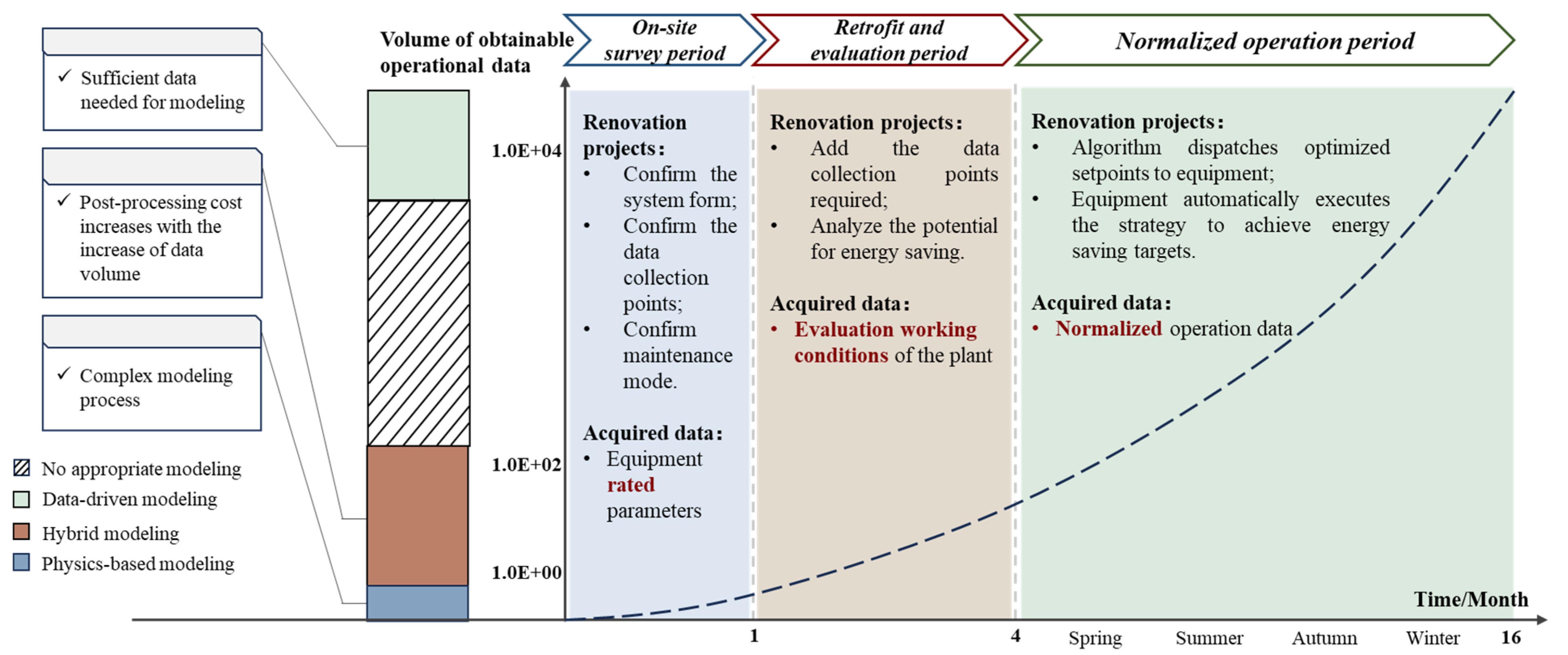
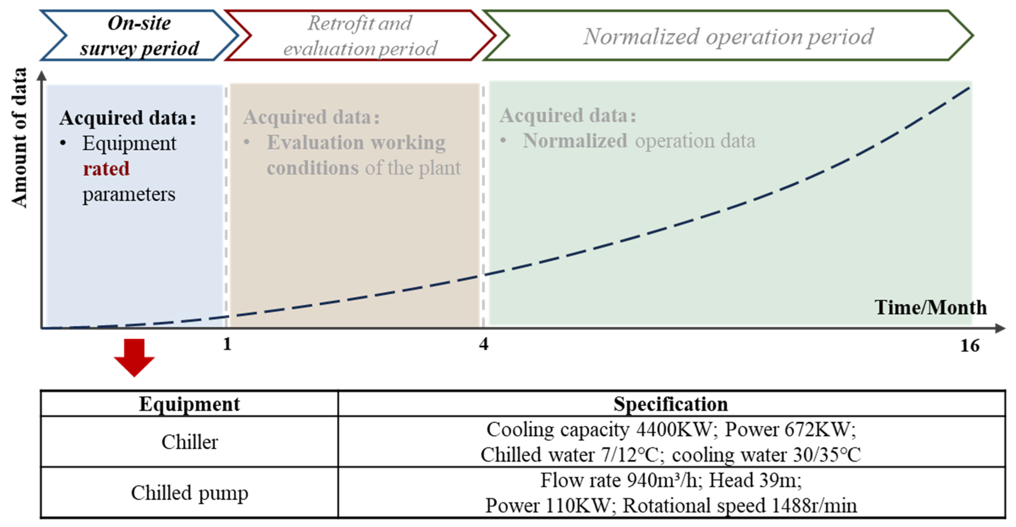
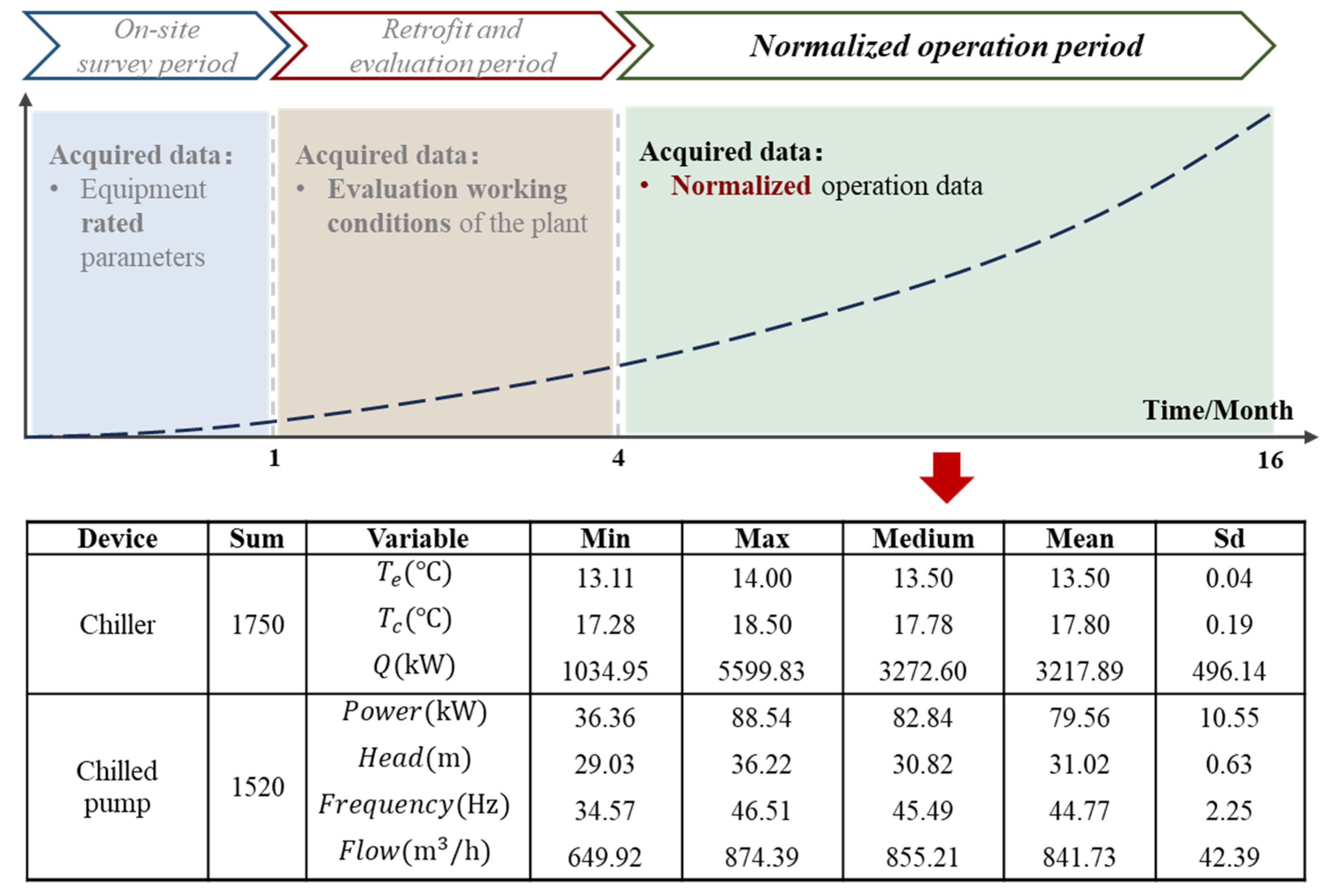
The energy-saving retrofitting of a chiller plant is a long-term project that consists of three stages. The duration from the start of the renovation to its completion was approximately one and a half years. Throughout the energy-saving renovation process, there were significant differences in the issues to be addressed and the data and information available at each stage, as represented in Figure 1.

2.1. On-Site Survey Period

This period was the stage of collecting materials and documents before the start of energy-saving retrofitting. (1) Moreover, it is necessary to collect the HVAC and automatic control drawings of the refrigeration plant to confirm the form of the HVAC system of the project, including the layout of the field equipment and the connection form between the equipment. (2) Additionally, it is necessary to confirm the distribution of operation data acquisition points and (3) to confirm the nameplate of each piece of equipment at the refrigeration plant site to obtain the rated operation parameters of the equipment. This stage typically lasts for one month. Only rated parameters were obtained for the equipment.

2.2. Retrofit and Evaluation Period

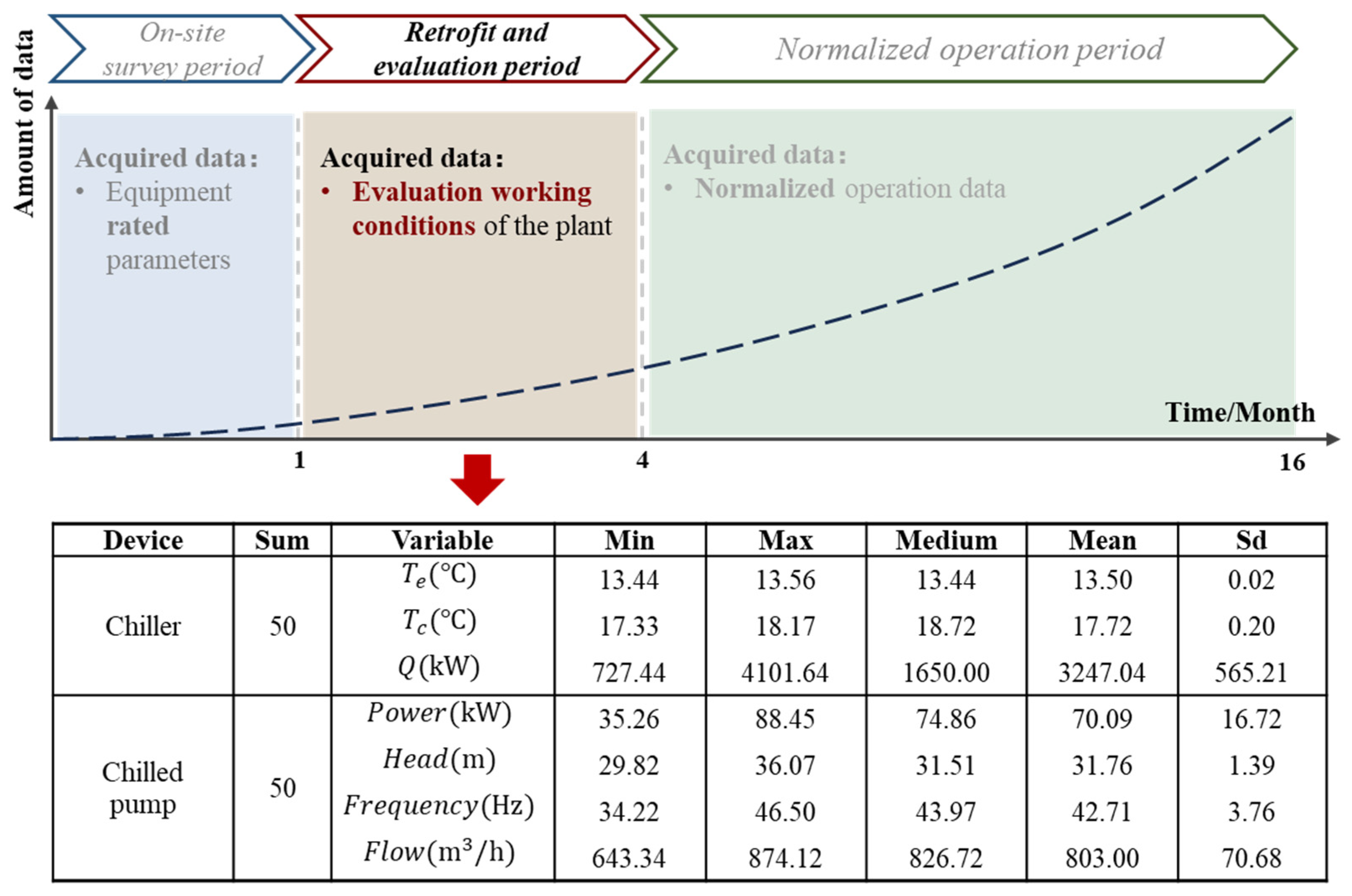
Here, we comprehensively evaluate the energy-saving potential of the target refrigeration plant and provide a retrofitting strategy. (1) The instantaneous operating conditions of the system under different load conditions, weather conditions, and terminal conditions are collected by repeatedly manually adjusting the operating state of the field equipment. (2) The working personnel record the data on energy-saving debugging conditions in real-time on the spot to tap the energy-saving limit conditions of the cooling plant and confirm its energy-saving potential. This stage typically lasts for a long period of time (typically approximately three months), and the amount of data that can be obtained is increased compared to that of the first stage.

2.3. Normalized Operation Period

After all energy-saving retrofit means are implemented, (1) the HVAC system is typically connected to an automatic data acquisition platform, and (2) the operation data of each device is automatically collected during the operation of the HVAC system to achieve a reliable and stable data acquisition method. The amount of data that could be obtained at this stage increased sharply compared to that of the previous two stages. However, as the running state of the equipment is often in the same interval under the same weather conditions, it is easy to encounter problems with single running data and serious homogenization in the early stages.

Under such a retrofit process, there is a contradiction between the difference in the amount of data that can be obtained for equipment modeling at different stages and the size of the data to which different modeling methods adapt. This leads to various disadvantages of a single modeling method at different stages of an energy-saving retrofit.

Table 1. Summary of mainstream equipment modeling methods.

Reference	Modeling Means	Component	Data Volume	Results
Kohlenbach and Ziegler (2008) [8]	Physics-based model	Single-effect LiBr/water absorption chillers	/	The dynamic agreement between experiment and simulation is with dynamic deviations around 10 s.
Lei and Zaheeruddin (2005) [6]	Physics-based model	Water chiller refrigeration system	/	The changes in water temperature take much longer to reach steady state in the system.
Kim and Park (2007) [36]	Physics-based model	Chiller	/	Study the transients of temperature, pressure, concentration, and void fraction of each component during the start-up operation.
Lu (2005) [7]	Physics-based model	All the energy consumption components	/	The physical limitations of the components and the interactions between components are embodied in the constraint section to complete the problem formulation of the proposed optimization.
Jin (2007) [24]	Hybrid model	Cooling tower	1440	The model can perfectly predict the cooling tower performance with RMSRE 0.048.
Niu (2023) [31]	Hybrid model	Chiller and pump	576	Considerable energy saving can be achieved by using the proposed simulation-based optimization method.
Deng (2023) [25]	Hybrid model	Chiller	420,480	The accuracy of the prediction model clearly increased, with R2 reaching 0.932.
Nedjah (2022) [37]	Hybrid model	Cooling tower	21,385	The tower effectiveness modeling occasioned an MSE of 3.5 and a R2 of 0.9924.
Kim (2019) [16]	Data-driven model	Chiller	3761	The developed chiller model was able to predict energy consumption with 99.07% accuracy.
Guo (2024) [22]	Data-driven model	Chiller	12,740	The established PGNN model complies with physical laws and has a much stronger out-of-sample generalization ability.
Chan (2022) [17]	Data-driven model	Chiller	9360	The implementation of the proposed control strategy enhanced system COP.
Bueso (2024) [19]	Data-driven model	Cooling tower	26,280	The MLP model has a better R2 value than the linear model.
Yu (2023) [35]	Physics-based model	Chiller and cooling tower	/	The neural network model has high accuracy; The hybrid model does not perform as well as the empirical model and the neural network model in terms of accuracy.
	Hybrid model		96
	Data-driven model		1308

summarizes the mainstream modeling methods and the amount of data to which they adapt.

The mainstream methods of equipment modeling are not fully applicable in the context of specific energy-saving renovation practices. (1) Data-driven modeling may encounter model blank periods when data are insufficient, and it cannot avoid the problem of model overfitting caused by data homogenization issues in the early stages of normal operation. (2) Parameter identification modeling is only suitable for cases with small sample sizes. In the later stages of energy-saving renovation, the modeling speed is decreased due to excessive data volume. (3) Although mechanism-based modeling can form models from the beginning of energy-saving renovation, as equipment usage time increases, the operational characteristics may deviate, thus making it difficult to ensure the accuracy of model predictions. Furthermore, the models formed by mechanism-based modeling are typically complex, ultimately increasing the cost of model utilization.

3. Proposal of a Phased Modeling Method for the Entire Retrofit Process

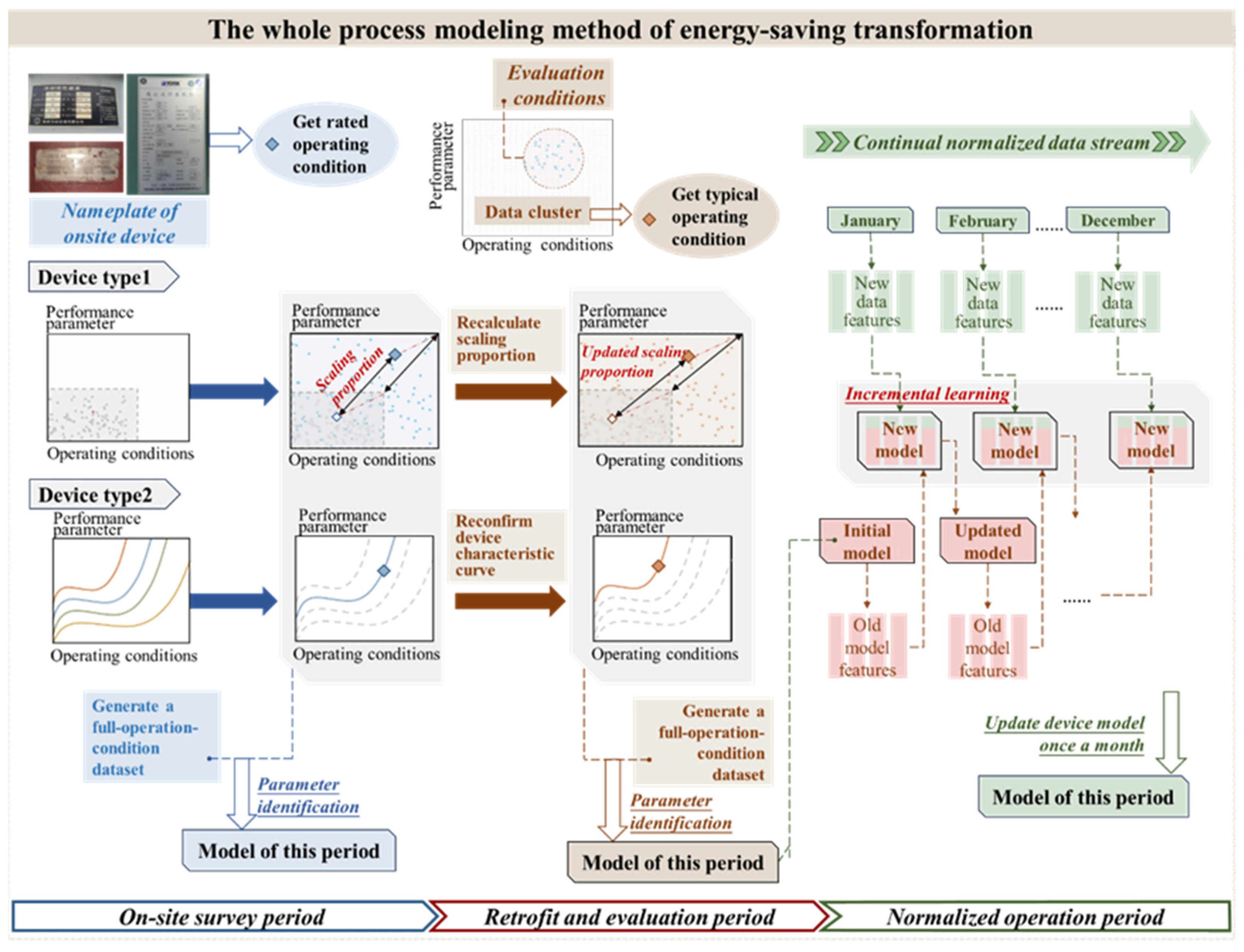
Against the background of the entire process of energy-saving retrofitting of refrigeration plants and aiming at the disadvantages of the existing equipment modeling methods, this study proposes a dynamic modeling method, as shown in Figure 2, which combines parameter identification with data driving and regularly updates the equipment model to reflect the current operation situation according to the data obtained at different stages. This ensures equipment models support optimal operation in all stages of energy-saving retrofitting.

To establish the equipment model, it was necessary to obtain the operation dataset of equipment covering the entire working condition interval. For equipment with different operating characteristics, different approaches are used to obtain operational data across the entire working condition range. Therefore, based on their operating characteristics, the equipment can be divided into two categories.

3.1. Type 1—Equipment with Unclear or Complicated Operation Characteristics

Equipment with operating characteristics and influence laws that are unclear or complicated includes chillers, heat pumps, cooling towers, and other equipment.

On-site survey period: Moreover, it is impossible to directly obtain the operation data for the entire working condition interval through the rated parameters. However, the operation state of the equipment under different working conditions is often included in the sample manual provided by the equipment manufacturer, and the dataset can be directly generated from the operation data of the entire working condition interval in the manual.

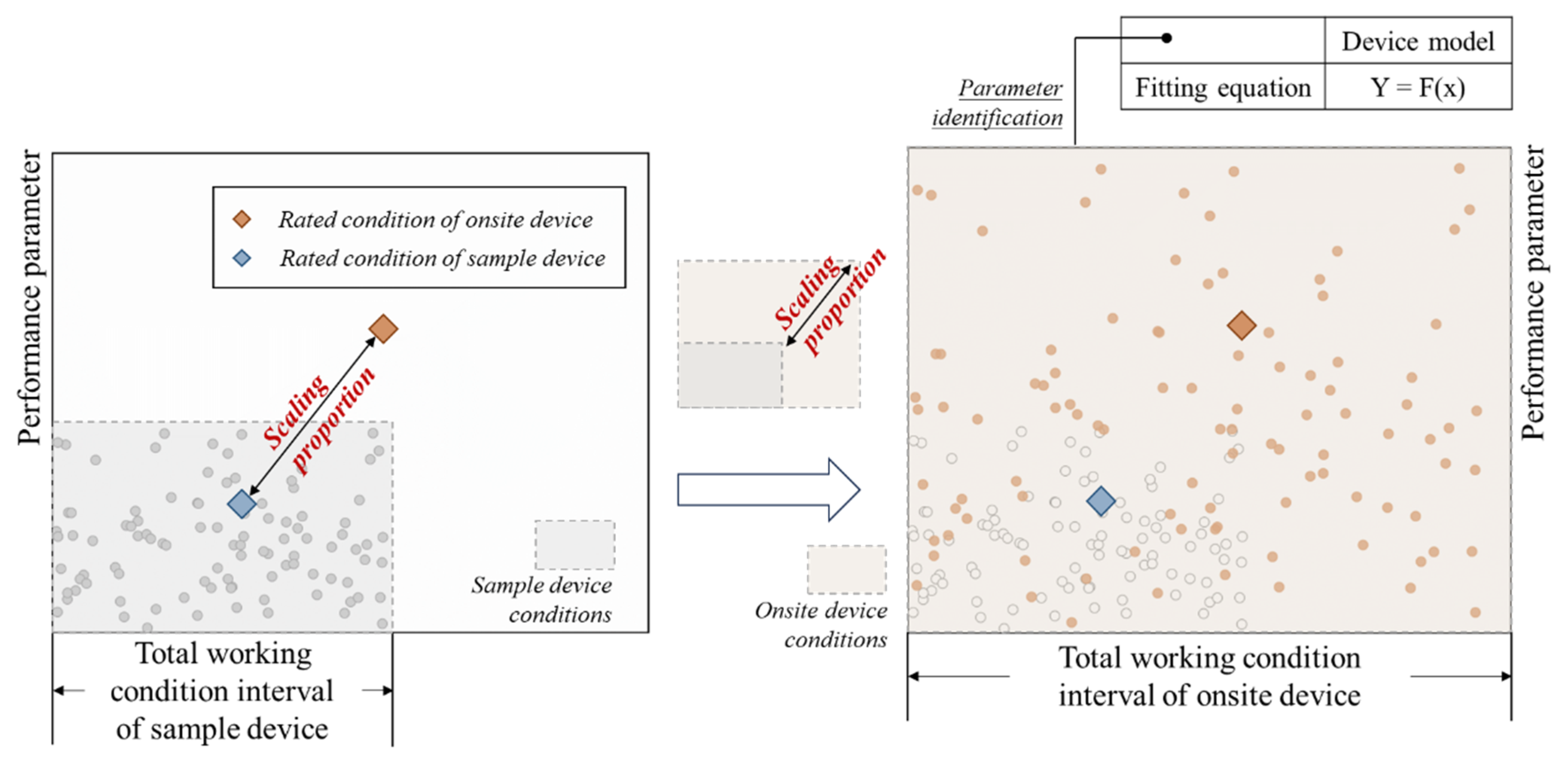
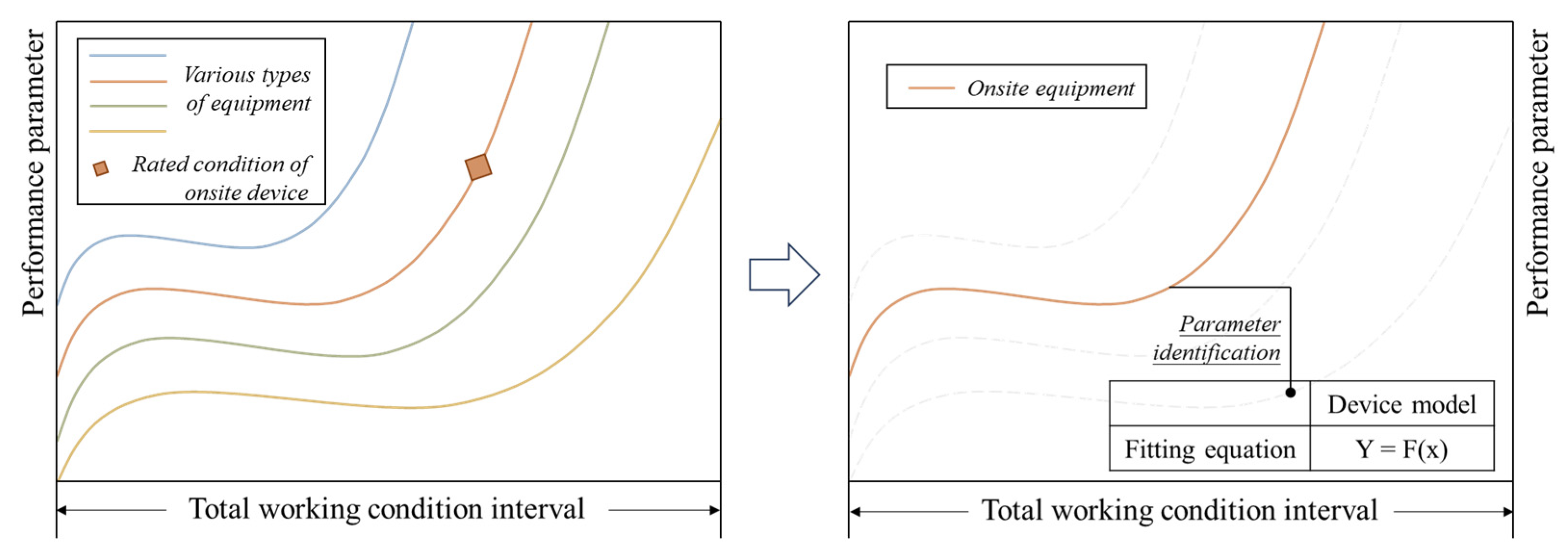
In practical engineering, issues with missing equipment documentation are commonly encountered due to irregular operation and maintenance (O&M) practices. When it is not possible to obtain manuals for onsite equipment, one can use the characteristic that equipment of the same type tends to exhibit similar performance. By collecting manuals for equipment of the same type, the operating data provided can be used as a general sample set for the on-site equipment. Then, using the rated operating characteristics of the on-site equipment as a reference, feature scaling can be applied to the general sample set, thus representing the full range of operating conditions for the on-site equipment with scaled data. This method provides a universal means of acquiring operating data across all operating conditions.

Although this stage has expanded data acquisition based on the rated parameters, the data volume still cannot support data-driven modeling. Therefore, appropriate parameter models were selected based on the obtained data, and the equipment performance model was acquired through parameter identification tailored to the specific characteristics of the equipment, as represented in Figure 3.

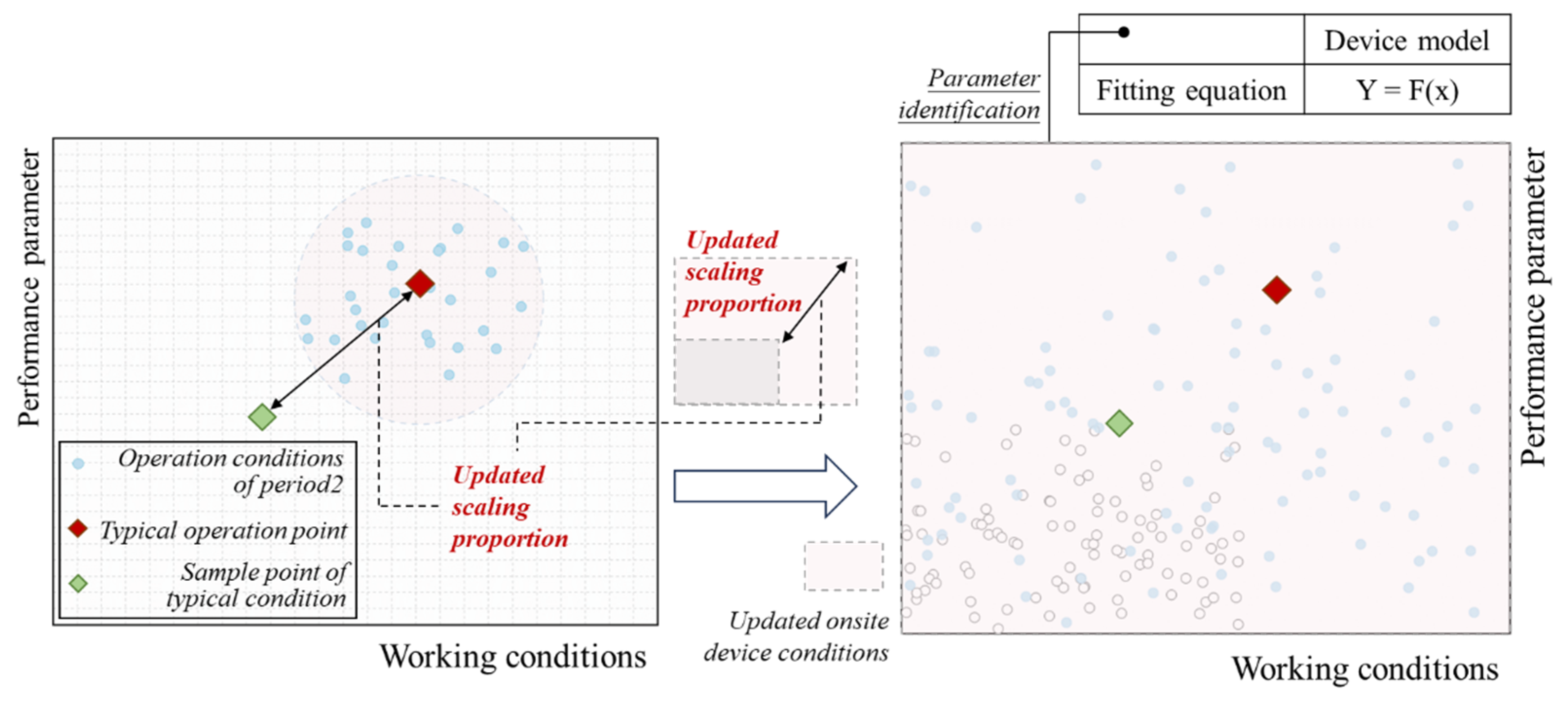
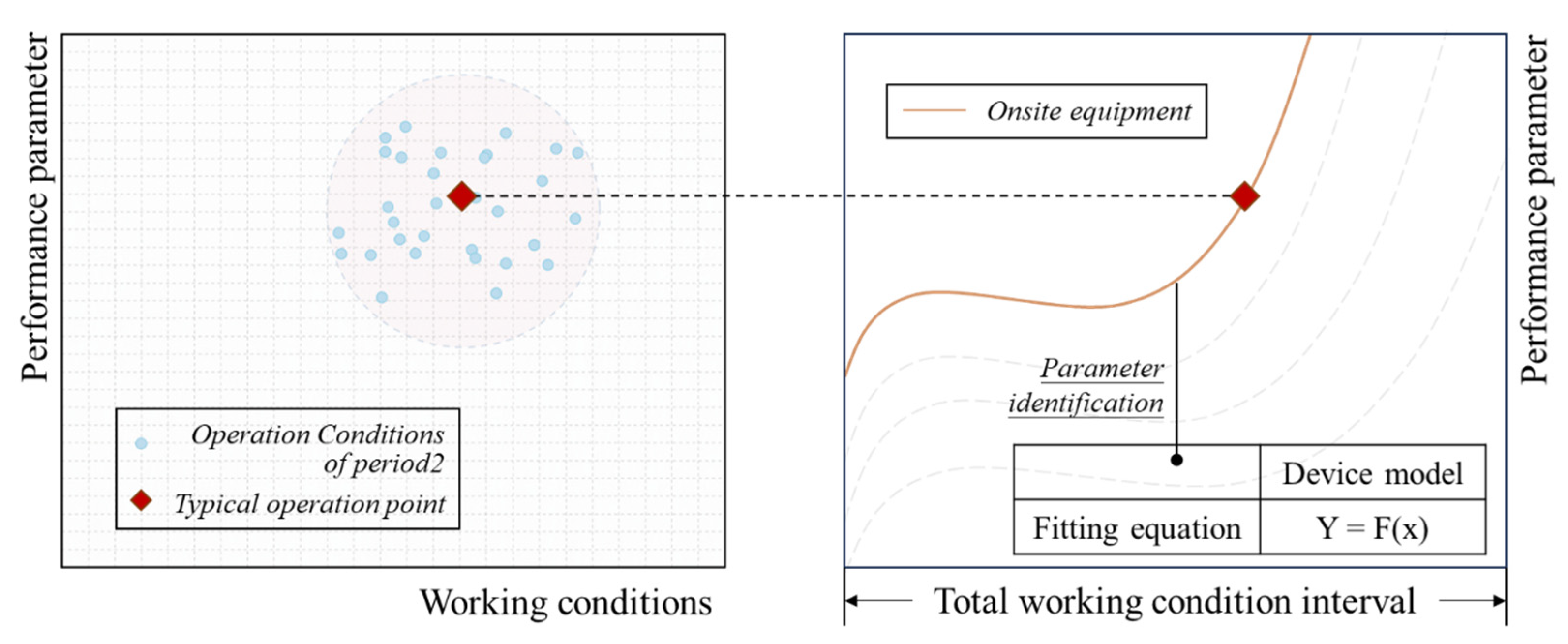
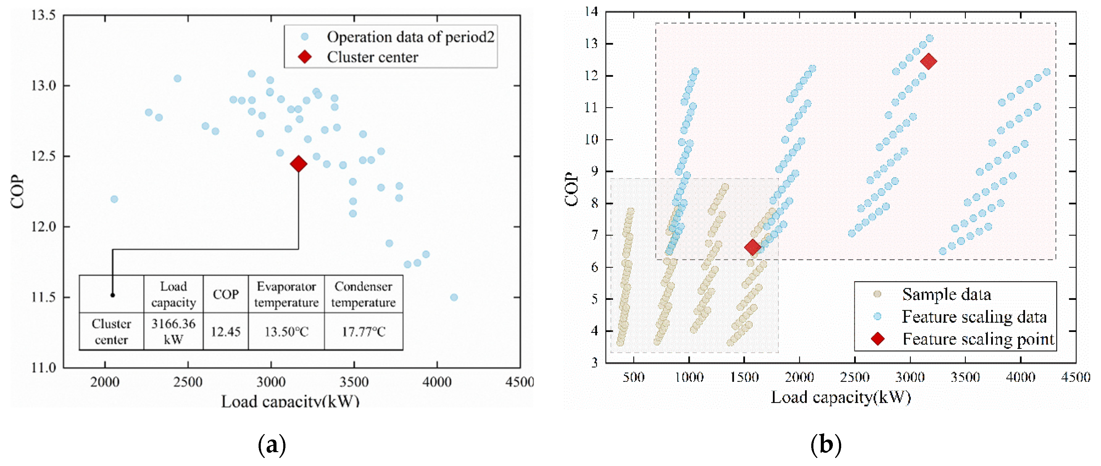
Retrofit and evaluation period: The operation data of the refrigeration plant in various typical terminal environments were obtained, and the collected data were often more representative of the actual operating condition interval of the equipment, which can cluster the working condition data collected from multiple fields of debugging into a typical working condition point. The idea of generating field equipment data points continues from the previous stage. If there is a sample manual of the corresponding equipment as a reference for the operation state of the entire operating range, the dataset will be generated based on the sample manual. If the sample manual cannot be obtained, the method of collecting samples of the same type of equipment will be adopted, and the typical operating points obtained by clustering will replace the rated parameters of the field equipment as the scaling characteristics. The general sample set will be scaled, as represented in Figure 4, and the scaled data will be used to represent the dataset of the entire operating range of the field equipment.

After obtaining the dataset, the equipment performance model was updated using parameter identification modeling.

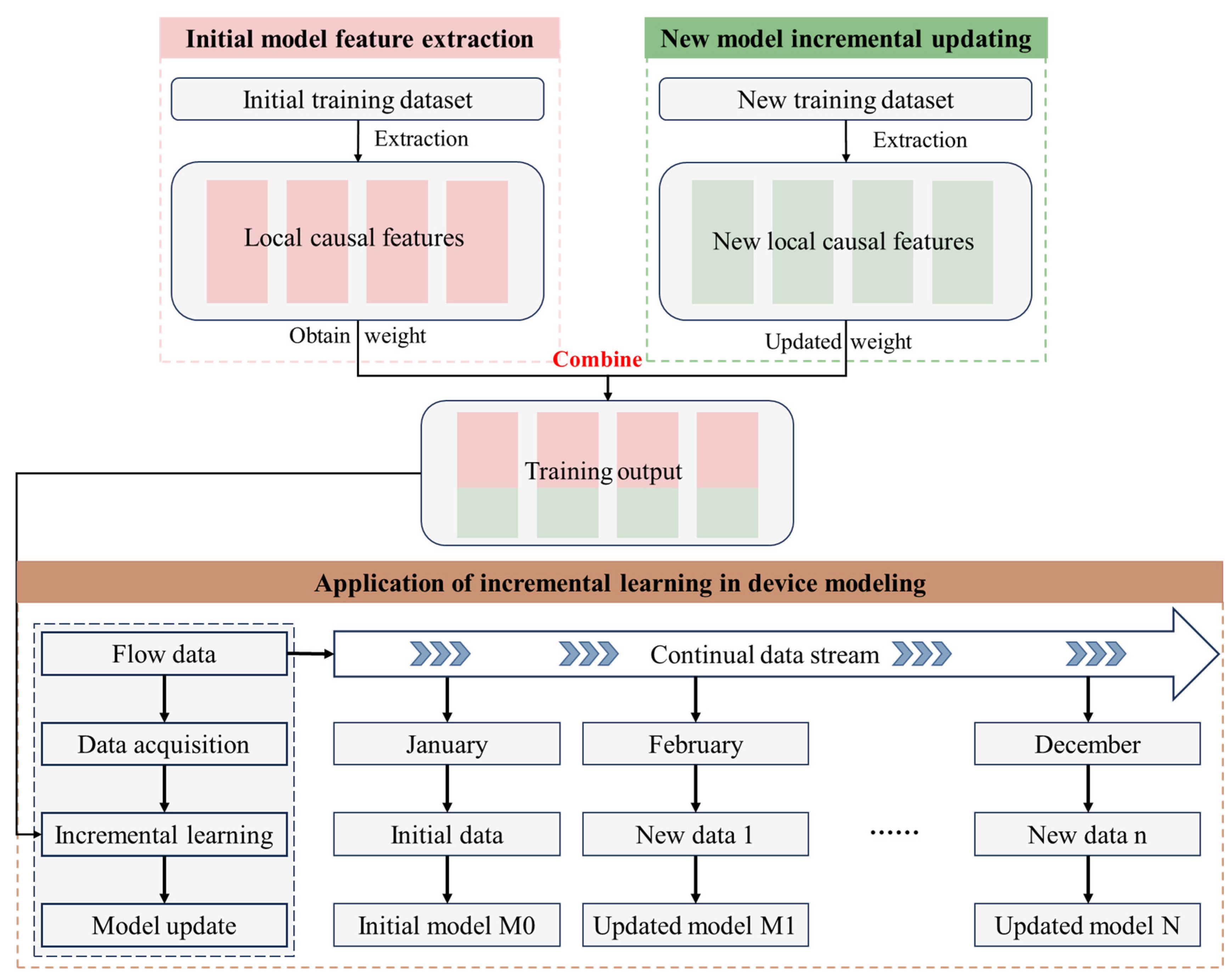
Normalized operation period: A large amount of actual operation data of the equipment is automatically collected, and the input of the latest operation data of the equipment can be continuously obtained. Compared to retraining the entire model, the incremental learning method can effectively use new data while retaining the characteristics of the existing model, thus saving time and computing resources. By continuously updating the model with real-time data, changes and trends in the operating characteristics of the equipment were promptly captured, thus ensuring that the model remained consistent with the actual conditions. The incremental learning process is represented in Figure 5.

3.2. Type 2—Equipment with Clear and Simple Operation Characteristics

This includes equipment with clear and simple operating characteristics and their influence on laws, such as a water pump.

On-site survey period: Using the given rated parameters of the equipment, the operation characteristic curve of the equipment was determined, and the operation data of the entire working condition interval were then deduced to generate the dataset, as represented in Figure 6. Based on the obtained data, an appropriate parameter model was selected according to the different equipment, and the equipment performance model was obtained by parameter identification modeling.

Retrofit and evaluation period: Similarly, the working condition data collected by field debugging numerous times are clustered into a typical working condition point, and the operating characteristic curve is corrected by using the data of this typical working condition point. Then, the operating data of the entire working condition interval is obtained in the same manner as in the previous stage to generate a dataset, as represented in Figure 7.

Then, the equipment model is updated using parameter identification.

Normalized operation period: Upon entering this stage, the approach for training the new models is identical to that of Type 1. Using the continuous input of new operational data, an incremental learning scheme was employed to update the model while retaining the existing data features. This ensures that the model adapts to changes in the operating characteristics of the equipment throughout its use.

Model performance validation against operational characteristics—including error metrics such as RMSE and CV—will be systematically evaluated in Section 4’s case study applications.

4. Application

4.1. Model Selection

This study was based on actual equipment data collected during an energy-saving renovation project at a low-efficiency data center. Using the modeling approach proposed in the previous section that was tailored to the entire energy-saving renovation process, models were developed for the actual equipment in the chiller plant of the data center. Type 1 equipment, exemplified by a chiller, and Type 2 equipment, represented by a chilled-water pump, were modeled separately. This study demonstrates the modeling of different types of equipment at each stage of the energy-saving renovation process to predict their operating performance, thus laying the foundation for the subsequent optimization of chiller plant operations.

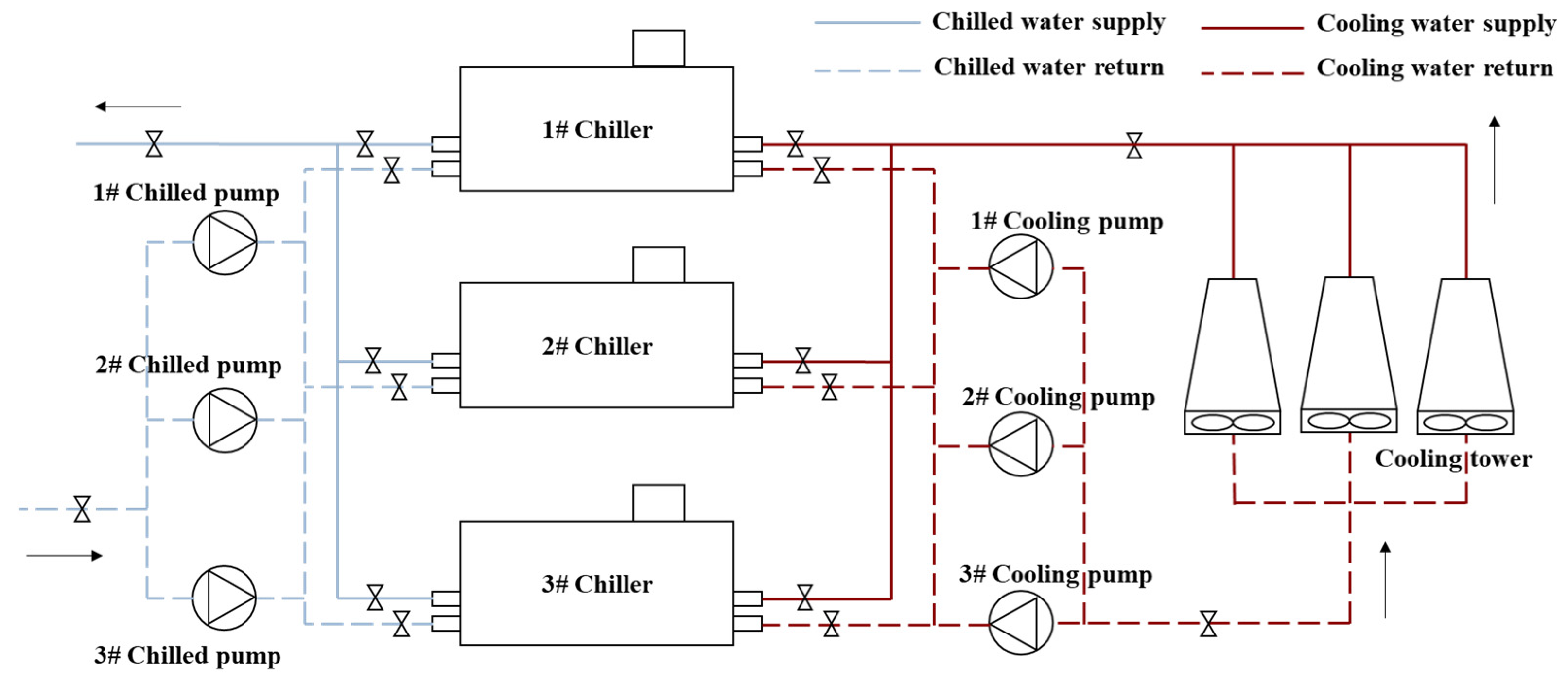
The cooling system of the refrigeration plant is represented in Figure 8.

4.1.1. Type1-Chiller

The chiller was modeled as a representative of Type 1. The chiller is often used as a cooling source in the refrigeration plant of a central air-conditioning system to provide chilled water for the terminal heat exchanger to control the indoor temperature while simultaneously using cooling water circulation to dissipate heat into the atmosphere through the cooling tower. The chiller used in this study is a centrifugal chiller, and the Coefficient of Performance (COP) is a key parameter that reflects its performance, as it is related to the energy consumption and efficiency of the chiller.

The definition of COP is as follows:

$$COP=Q_{chiller}/W_{total}$$

(1)

Many scholars have studied empirical models of chillers, and Lee et al. [38] evaluated the performance prediction ability and model applicability of 11 mixed models based on empirical formulas for centrifugal chillers. Based on the results of their research and the practical applicability of the model, a multivariate polynomial regression model (MP model) was selected for this project as the basis for chiller modeling.

$$COP=a_1+a_2\times Q+a_3\times T_c+a_4\times T_e+a_5\times Q^2+a_6\times {T_c}^2+a_7\times {T_e}^2+a_8\times T_c\times Q+a_9\times T_e\times Q+a_{10}\times T_c\times T_e$$

(2)

where $a_1-a_{10}$ are constants; $Q$ is the load capacity ($\mathrm{k}\mathrm{W}$); $T_e$ is the evaporator temperature ($°\mathrm{C}$); and $T_c$ is the condenser temperature ($°\mathrm{C}$).

4.1.2. Type2-Chilled Pump

The water pump is an important component of the cooling system that provides power to the system to overcome the resistance of the pipe network. Moreover, its head directly determines if the water demand of the entire system can be met. The characteristic curve of a water pump is the most accurate and effective method for determining the performance of the water pump. When establishing the pump model, the characteristic curve of the pump is transformed into a functional form that is convenient to solve and calculate.

For the common variable-frequency water pump, considering that there are similar laws among flow, head, power, efficiency, and speed and that the speed of the pump is typically changed by variable-frequency speed regulation, the model can be written as follows:

$$\begin{array}{c}\left\{\begin{array}{c}H=a_1\ast Q^2+a_2\ast Q\ast \left(f/f_0\right)+a_3\ast {\left(f/f_0\right)}^2\\ W=b_1\ast Q^2\ast \left(f/f_0\right)+b_2\ast Q\ast {\left(f/f_0\right)}^2+b_3\ast {\left(f/f_0\right)}^3\end{array}\right.\end{array}$$

(3)

where a and b are constants; $Q$ is the pump flow (${\mathrm{m}}^3/\mathrm{h}$); H is the pump head (m); W is the pump power (kW); $f$ is the pump frequency (Hz); and $f_0$ is the rated frequency of the pump (Hz).

4.2. Model Establishment

After selecting the appropriate foundational model during the actual energy-saving retrofit, the process involved establishing the initial model and gradually updating it based on operational data following the different stages of project advancement, thereby enhancing the predictive accuracy of the model.

4.2.1. On-Site Survey Period

During the initial site inspection stage of the energy-saving retrofit, the rated parameters of the water chillers and chilled-water pumps used in this project were collected, as represented in Figure 9.

• Type1-Chiller

Due to their unclear operational characteristics that cannot be deduced from the rated parameters and considering the considerable age of chiller plants, obtaining sample manuals for chillers is challenging. Therefore, during the onsite survey phase, it was necessary to collect sample manuals for all chiller units of the same type. This manual serves as a sample reference benchmark for the characteristic variations in centrifugal chiller units under different operating conditions. The rated operating conditions of the prototype selected for renovation are listed in

Table 2. The rated parameters of the sample chiller.

Equipment	Specification
Sample Chiller	Cooling capacity 1832 KW; Power 412 KW; Chilled water 7/12 °C; cooling water 30/35 °C

.

The scaling ratio for the operating conditions of the sample chiller unit was determined by calculating the ratio of the COP at the rated conditions between the on-site chiller and the sample chiller:

$$scaling ratio={\displaystyle \frac{COP of onsite chiller at rated oprating condition}{Catalog chiller COP}}=1.47$$

(4)

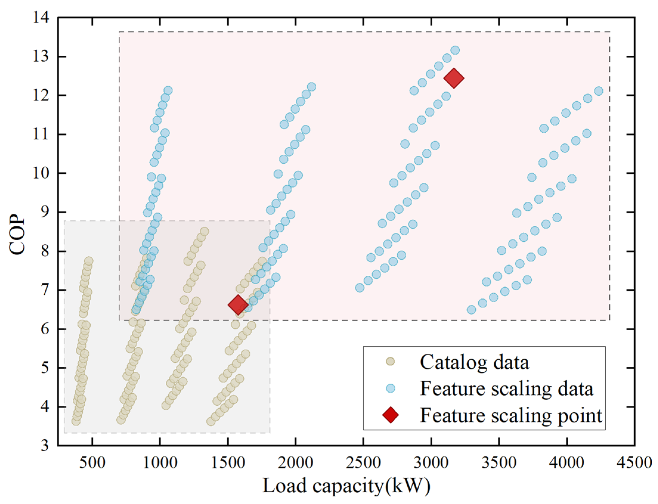
Based on this ratio, the COP values of the sample points under all operating conditions were scaled down, and the COP values of the onsite chiller under different evaporator temperatures, condenser temperatures, and the Partial Load Ratio (PLR) were obtained to represent the full operating data of the field cooler.

The feature scaling process is illustrated in Figure 10.

The same cluster points in the figure share the same PLR. The points arranged in close rows in the same cluster possess the same evaporator temperature, whereas the points arranged in loose rows in the same cluster possess the same condenser temperature.

As there are numerous items involved in the MP model; based on this dataset, LASSO regression was used to screen variables and obtain the regression coefficient of each item. LASSO regression is a commonly used the linear regression method and technique for feature selection and regularization. By imposing penalties on the coefficient vectors to achieve sparsity, certain coefficients were compressed to zero, thereby achieving variable selection and model simplification.

The model formula for the chiller during the onsite survey period was obtained as in

Table 3. The model formula of the chiller in the onsite-survey period.

	${\mathit{a}}_{\mathsf{1}}$	${\mathit{a}}_{\mathsf{2}}$	${\mathit{a}}_{\mathsf{3}}$	${\mathit{a}}_{\mathsf{4}}$	${\mathit{a}}_{\mathsf{5}}$	${\mathit{a}}_{\mathsf{6}}$	${\mathit{a}}_{\mathsf{7}}$	${\mathit{a}}_{\mathsf{8}}$	${\mathit{a}}_{\mathsf{9}}$	${\mathit{a}}_{\mathsf{10}}$
Parameter value	$11.42$	$7.55\times {10}^{-4}$	0	$-2.6\times {10}^{-1}$	$-1.30\times {10}^{-7}$	$2.17\times {10}^{-3}$	$6.68\times {10}^{-3}$	$-4.95\times {10}^{-6}$	$2.16\times {10}^{-5}$	$-4.68\times {10}^{-4}$
Formula	$\begin{array}{c}COP=11.42+\left(7.55\times {10}^{-4}\right)\times Q-\left(2.6\times {10}^{-1}\right)\times T_c-\left(1.30\times {10}^{-7}\right)\times Q^2+\left(2.17\times {10}^{-3}\right)\times {T_c}^2+\left(6.68\times {10}^{-3}\right)\times {T_e}^2\\ -\left(4.95\times {10}^{-6}\right)\times T_c\times Q+\left(2.16\times {10}^{-5}\right)\times T_e\times Q-(4.68\times {10}^{-4})\times T_c\times T_e\end{array}$

.

• Type2-Chilled pump

The specific speed [39] of a water pump significantly influences its operating characteristics. Specific speed is an important parameter for describing the geometric shape and operating performance of a water pump. Moreover, it is defined as the speed at a unit flow rate and is typically used to characterize the size and performance of a water pump. The specific speed of the water pump was calculated using the following formula:

$$n_s=3.65n\sqrt{Q}/H^{\raisebox{1ex}{$3$}\!\left/ \!\raisebox{-1ex}{$4$}\right.}$$

(5)

where $n_s$ is the specific speed; $n$ is the speed of the water pump; $Q$ is the pump flow rate (${\mathrm{m}}^3/\mathrm{s}$); and $H$ is the pump head (m).

The specific speed of the water pump in the cooling system is calculated as follows:

$$n_s=3.65n\sqrt{Q}/H^{\raisebox{1ex}{$3$}\!\left/ \!\raisebox{-1ex}{$4$}\right.}={\displaystyle \frac{3.65\times 1488\times \sqrt{940/3600}}{{39}^{\raisebox{1ex}{$3$}\!\left/ \!\raisebox{-1ex}{$4$}\right.}}}=177.79$$

(6)

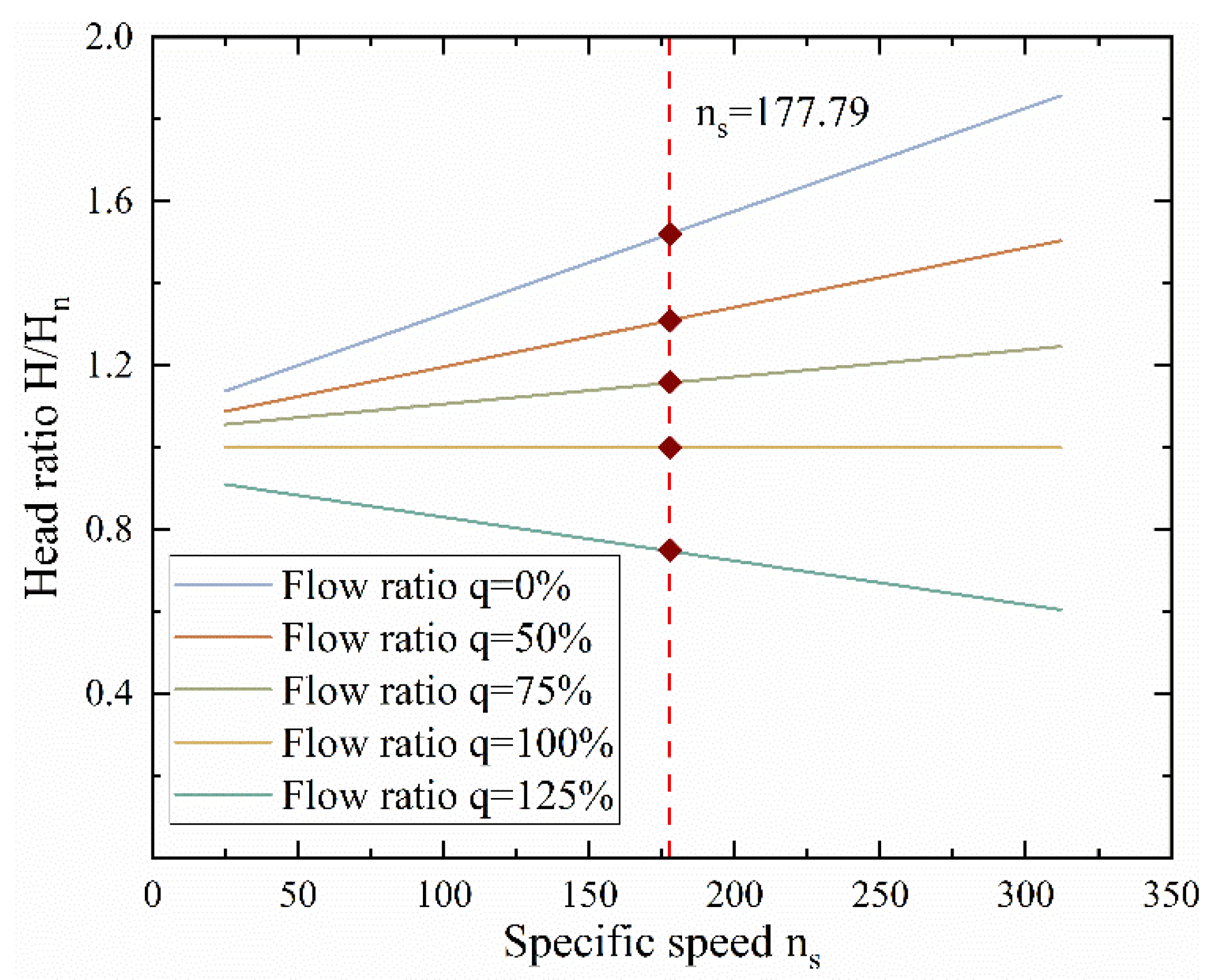
The relationship between the specific speed and head ratio of a general centrifugal pump under different flow ratios is represented in Figure 11.

Based on the calculated $n_s$, head-to-rated-head ratios ($H/H\text{\_}rated$) at discrete flow points ($q=0\%,50\%,75\%,100\%,125\%$) were obtained from the normalized pump performance curves in Figure 11.

Frequency values were derived via the affinity law:

$$\begin{array}{c}f/f\text{\_}rated =q/Q\text{\_}rated \end{array}$$

(7)

where $f\text{\_}rated$ is the rated frequency.

Based on the head and flow rate parameters, the pump power can be calculated using the following formula:

$$\begin{array}{c}P = \rho gQH/\eta \end{array}$$

(8)

where η is the efficiency of pump, simplified as 0.8.

A dataset was generated from the five working conditions, as listed in

Table 4. Dataset of the chilled water pump under 5 different flows.

	Head (m)	Flow (${\mathbf{m}}^{\mathsf{3}}\mathsf{/}\mathbf{h}$)	Frequency (Hz)	Power (kW)
A1	59.3	235	12.5	37.9
A2	50.7	470	25.0	64.8
A3	46.0	705	37.5	88.3
A4	39.0	940	50.0	99.8
A5	29.6	1175	62.5	94.7

.

Based on this dataset, all regression parameters of the model are obtained by the ordinary least squares method that minimizes the sum of squares of residuals, and the model formula of the chilled water pump in the onsite survey period can be obtained as in

Table 5. The model formula of the chilled water pump in the onsite survey period.

	${\mathit{a}}_{\mathsf{1}}$	${\mathit{a}}_{\mathsf{2}}$	${\mathit{a}}_{\mathsf{3}}$	${\mathit{b}}_{\mathsf{1}}$	${\mathit{b}}_{\mathsf{2}}$	${\mathit{b}}_{\mathsf{3}}$
Parameter value	$-(1.26\times {10}^{-5})$	$-0.01$	59.18	$-\left(3.83\times {10}^{-5}\right)$	$0.09$	$55.70$
Formula	$\left\{\begin{array}{c}H=-\left(1.26\times {10}^{-5}\right)\ast Q^2-0.01\ast Q\ast \left(f/f_0\right)+59.18\ast {\left(f/f_0\right)}^2\\ W=-\left(3.83\times {10}^{-5}\right)\ast Q^2\ast \left(f/f_0\right)+0.09\ast Q\ast {\left(f/f_0\right)}^2+55.70\ast {\left(f/f_0\right)}^3\end{array}\right.$

.

4.2.2. Retrofit and Evaluation Period

During this period, it was necessary to manually adjust the refrigeration plant frequently to test its operating conditions under various conditions.

Fifty sets of data were collected from the site under different working conditions. Figure 12 represents the comprehensive statistics of the collected data, including the minimum, maximum, median, mean, and standard deviation.

• Type1-Chiller

The clustering of the collected working conditions into a typical working condition is represented in Figure 13.

Then, referring to the rated operating point of the prototype and the typical operating point obtained by clustering, the COP ratio of the two under the same operating conditions (evaporator temperature, condenser temperature, and PLR) is obtained.

$$\begin{array}{c}new scaling ratio={\displaystyle \frac{COP of onsite chiller at typical oprating condition}{COP of sample chiller at typical oprating condition}}=1.86\end{array}$$

(9)

Based on the new ratio, the COP values of the sample points under all operating conditions were scaled down, and the COP values of the field chillers under different evaporator temperatures, condenser temperatures, and PLR were obtained, as represented in Figure 13b. The obtained data represents the full operating data of the onsite chillers.

Based on this dataset, the variables were screened using LASSO regression; the regression coefficient of each item was obtained; and the model formula of the chiller in the retrofit and evaluation periods is represented in

Table 6. The model formula of the chiller in the retrofit and evaluation period.

	${\mathit{a}}_{\mathsf{1}}$	${\mathit{a}}_{\mathsf{2}}$	${\mathit{a}}_{\mathsf{3}}$	${\mathit{a}}_{\mathsf{4}}$	${\mathit{a}}_{\mathsf{5}}$	${\mathit{a}}_{\mathsf{6}}$	${\mathit{a}}_{\mathsf{7}}$	${\mathit{a}}_{\mathsf{8}}$	${\mathit{a}}_{\mathsf{9}}$	${\mathit{a}}_{\mathsf{10}}$
Parameter value	$14.45$	$1.16\times {10}^{-3}$	$-3.49\times {10}^{-1}$	$1.89\times {10}^{-1}$	$-2.35\times {10}^{-7}$	$2.78\times {10}^{-3}$	$-6.65\times {10}^{-3}$	$-7.39\times {10}^{-6}$	$3.01\times {10}^{-5}$	$8.90\times {10}^{-4}$
Formula	$\begin{array}{c}COP=14.45+\left(1.16\times {10}^{-3}\right)\times Q-\left(3.49\times {10}^{-1}\right)\times T_c+\left(1.89\times {10}^{-1}\right)\times T_e-\left(2.35\times {10}^{-7}\right)\times Q^2\hfill \\ \hspace{1em}\hspace{1em}\hspace{1em}\hspace{1em}\hspace{1em}\hspace{1em}\hspace{1em}+\left(2.78\times {10}^{-3}\right)\times {T_c}^2-\left(6.65\times {10}^{-3}\right)\times {T_e}^2-\left(7.39\times {10}^{-6}\right)\times T_c\times Q+\left(3.01\times {10}^{-5}\right)\times T_e\times Q\hfill \\ \hspace{1em}\hspace{1em}\hspace{1em}\hspace{1em}\hspace{1em}\hspace{1em}\hspace{1em}+(8.90\times {10}^{-4})\times T_c\times T_e\hfill \end{array}$

.

• Type2-Chilled pump

During the retrofitting and evaluation periods, adjusting the equipment speed ratios involves intricate internal mechanical structures, thus making it impractical to correct them based on the collected test data. Additionally, the quantity of collected pump operation data was insufficient to support the incremental learning of the model. Therefore, at this stage, the pump model obtained during the on-site survey phase was used, as represented in

Table 7. The model formula of the chilled water pump in the retrofit and evaluation period.

	${\mathit{a}}_{\mathsf{1}}$	${\mathit{a}}_{\mathsf{2}}$	${\mathit{a}}_{\mathsf{3}}$	${\mathit{b}}_{\mathsf{1}}$	${\mathit{b}}_{\mathsf{2}}$	${\mathit{b}}_{\mathsf{3}}$
Parameter value	$-1.26\times {10}^{-5}$	$-0.01$	59.18	$-3.83\times {10}^{-5}$	$0.09$	$55.70$
Formula	$\left\{\begin{array}{c}H=-\left(1.26\times {10}^{-5}\right)\ast Q^2-0.01\ast Q\ast \left(f/f_0\right)+59.18\ast {\left(f/f_0\right)}^2\\ W=-\left(3.83\times {10}^{-5}\right)\ast Q^2\ast \left(f/f_0\right)+0.09\ast Q\ast {\left(f/f_0\right)}^2+55.70\ast {\left(f/f_0\right)}^3\end{array}\right.$

.

4.2.3. Normalized Operation Period

After connecting to an automatic data acquisition system, data were collected every 15 min. The operational data for each piece of equipment at the chiller plant in October 2023 was collected and cleaned, as represented in Figure 14.

• Type1-Chiller

Considering 80% of the data as the training set and 20% of the data as the test set, and considering the chiller model obtained in the previous stage as the basic model, the model parameters were updated every month using small-batch learning. In this case, the model in the retrofit and evaluation stages was updated using the dataset from October, and the final model, obtained by adjusting the learning rate and the number of iterations, is presented in

Table 8. The model formula of the chiller in October 2023.

	${\mathit{a}}_{\mathsf{1}}$	${\mathit{a}}_{\mathsf{2}}$	${\mathit{a}}_{\mathsf{3}}$	${\mathit{a}}_{\mathsf{4}}$	${\mathit{a}}_{\mathsf{5}}$	${\mathit{a}}_{\mathsf{6}}$	${\mathit{a}}_{\mathsf{7}}$	${\mathit{a}}_{\mathsf{8}}$	${\mathit{a}}_{\mathsf{9}}$	${\mathit{a}}_{\mathsf{10}}$
Parameter value	$6.03$	$6.37\times {10}^{-4}$	0	$-1.26\times {10}^{-1}$	$-1.30\times {10}^{-7}$	$2.17\times {10}^{-3}$	$6.68\times {10}^{-3}$	$-4.95\times {10}^{-6}$	$2.16\times {10}^{-5}$	$-4.68\times {10}^{-4}$
Formula	$\begin{array}{c}COP=6.03+\left(6.37\times {10}^{-4}\right)\times Q-\left(1.26\times {10}^{-3}\right)\times T_c-\left(1.30\times {10}^{-7}\right)\times Q^2+\left(2.17\times {10}^{-3}\right)\times {T_c}^2\hfill \\ \hspace{1em}\hspace{1em}\hspace{1em}\hspace{1em}\hspace{1em}\hspace{1em}\hspace{1em}+\left(6.68\times {10}^{-3}\right)\times {T_e}^2-\left(4.95\times {10}^{-6}\right)\times T_c\times Q+\left(2.16\times {10}^{-5}\right)\times T_e\times Q\hfill \\ \hspace{1em}\hspace{1em}\hspace{1em}\hspace{1em}\hspace{1em}\hspace{1em}\hspace{1em}-(4.68\times {10}^{-4})\times T_c\times T_e\hfill \end{array}$

.

• Type2-Chilled pump

The chilled-water pump model is updated in the same manner to obtain the formula for the normalized period of October, as represented in

Table 9. The model formula of the chilled water pump in the normalized operation period.

	${\mathit{a}}_{\mathsf{1}}$	${\mathit{a}}_{\mathsf{2}}$	${\mathit{a}}_{\mathsf{3}}$	${\mathit{b}}_{\mathsf{1}}$	${\mathit{b}}_{\mathsf{2}}$	${\mathit{b}}_{\mathsf{3}}$
Parameter value	$-7.61\times {10}^{-6}$	$-0.01$	59.18	$-3.40\times {10}^{-5}$	$0.09$	$55.70$
Formula	$\left\{\begin{array}{c}H=-(7.61\times {10}^{-6})\ast Q^2-0.01\ast Q\ast \left(f/f_0\right)+59.18\ast {\left(f/f_0\right)}^2\\ W=-(3.40\times {10}^{-5})\ast Q^2\ast \left(f/f_0\right)+0.09\ast Q\ast {\left(f/f_0\right)}^2+55.70\ast {\left(f/f_0\right)}^3\end{array}\right.$

.

4.3. Model Validation

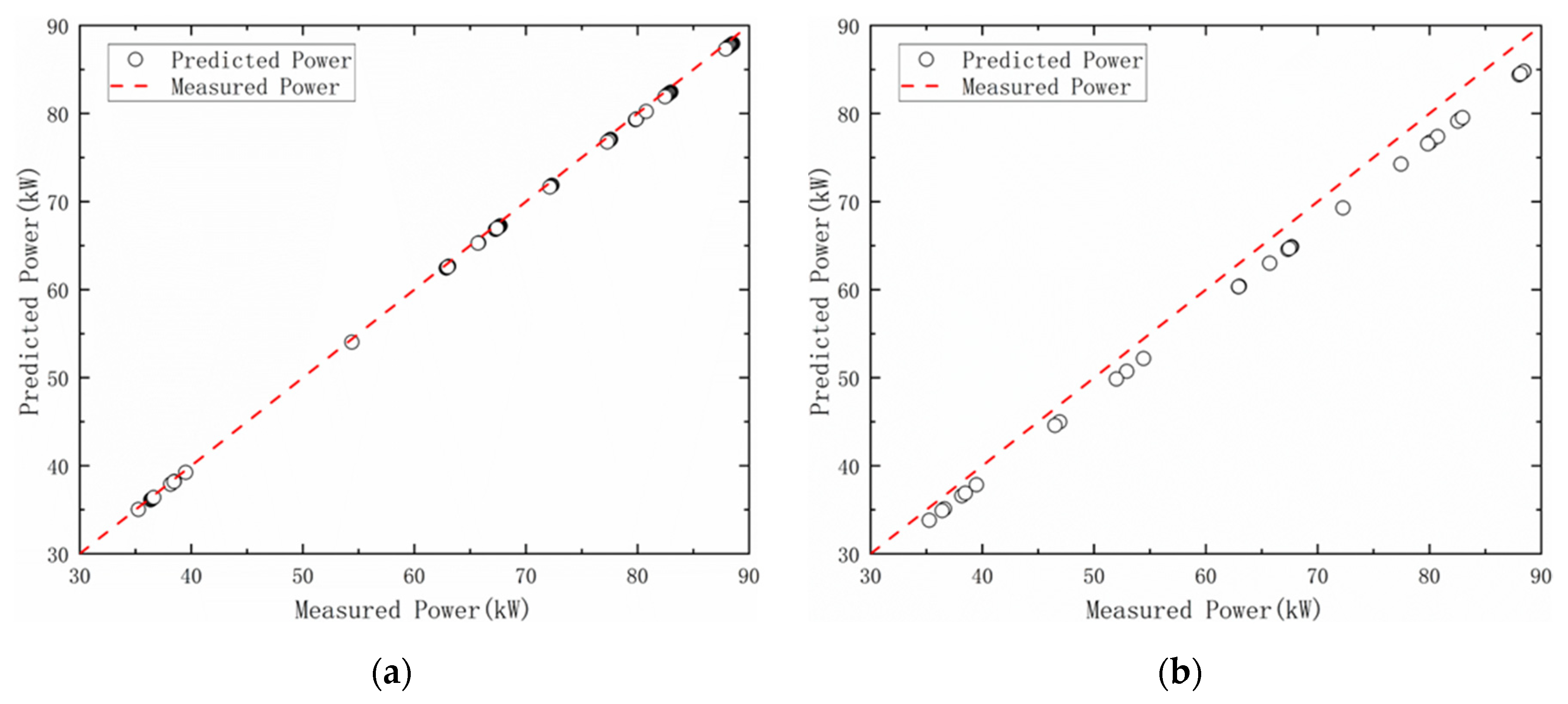
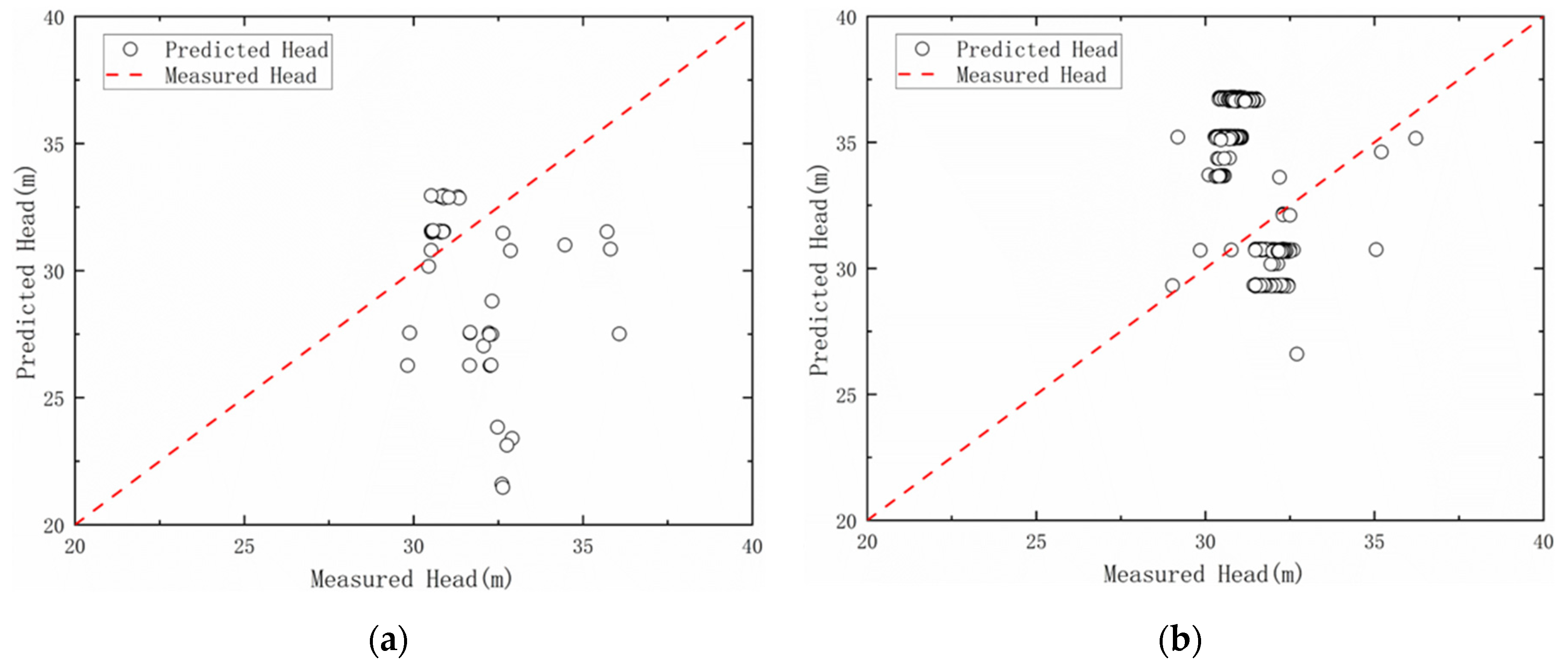
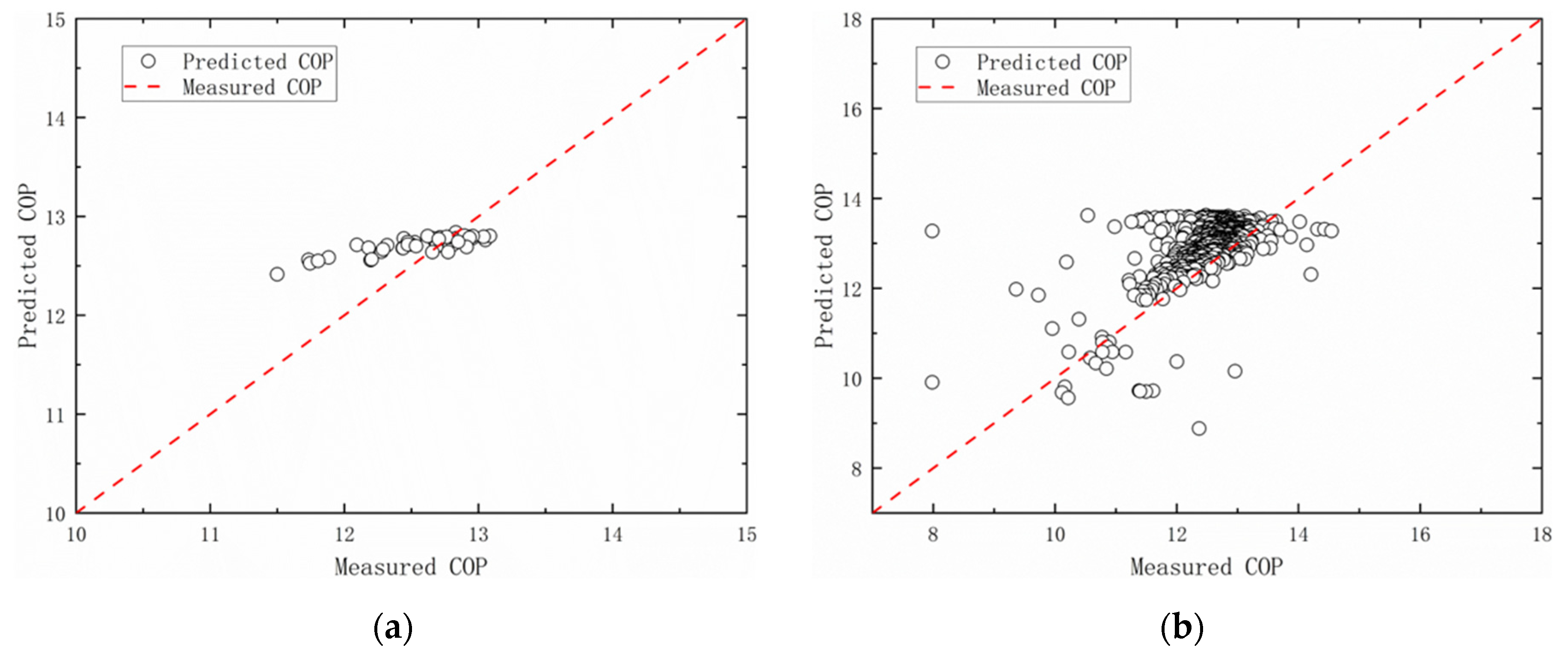
Figure 15, Figure 16 and Figure 17 compare the differences between the predicted values based on the model established using the method proposed in this study and the actual operational data at different stages of the energy-saving retrofit for the chiller unit and the chilled water pump. The horizontal axis represents the measured performance, and the vertical axis represents the predicted performance. Each circle represents a set of data-prediction results. The diagonal line in the center represents an ideal prediction, where the predicted value equals the measured value. In Figure 15 and Figure 16, the fitting situation of the P-Q and H-Q models of the chilled-water pump is described during the retrofit, evaluation, and normalized operation periods. Figure 17 represents the performance of the COP model for the chiller.

To quantitatively describe the quality and accuracy of these models, two evaluation indices, including the mean square error (RMSE) and the root mean square coefficient of variation (CV), were introduced. The parameters are defined as follows:

$$\begin{array}{c}RMSE=\sqrt{{\displaystyle \frac{\sum {({\widehat{y}}_i-y_i)}^2}{n}}}\end{array}$$

(10)

$$\begin{array}{c}CV={\displaystyle \frac{RMSE}{\left|\sum \frac{y}{n}\right|}}\times 100\end{array}$$

(11)

RMSE represents the error between the predicted and measured values and represents the accuracy of the model. A smaller MSE value indicates better model accuracy. The CV was used to indicate the degree of fit of a model to all measured data. A smaller CV value was indicative of a better model. In practical applications, an equipment prediction model with 3–5% CV is considered acceptable. In this study, a CV value of 5% was used as the acceptable range for judging the model.

Table 10. CV and RMSE of device models in different periods.

Device		Period	CV	RMSE
Chiller COP model		Energy-saving assessment	6.879	0.856
		Normalized operation	4.729	0.594
Chilled pump	H-Q model	Energy-saving assessment	21.755	6.282
		Normalized operation	14.647	4.541
	P-Q model	Energy-saving assessment	4.245	2.975
		Normalized operation	0.665	0.537

compares the accuracy of different equipment models in the retrofit and evaluation periods and the normalized operation period.

For the equipment model established according to the method proposed in this study, when compared vertically in the process of energy-saving retrofitting, the CV value gradually decreases, and with an increase in the amount of data used for modeling, the model gradually tends to be accurate. The model did not perform well on the H-Q model of the chilled water pump, and the CV value of the model exhibited a large gap with an acceptable range of 5% during the entire retrofitting process. The chilled water pump model’s underperformance originates from field instrumentation constraints that necessitated proxy pressure variables. This substitution introduced inherent input inaccuracies, rendering the model unsuitable for optimization—a limitation resolved through its exclusion from downstream analyses, based on which, the model will not be included in the discussion in the follow-up discussion. Future deployments will resolve such issues through direct pressure sensing and transfer learning from instrumented reference systems.

For two types of equipment with different operating characteristics, the modeling scheme proposed in this study exhibited good prediction accuracy. The CV values of the two equipment models in the normal operation stage and the chilled water pump model in the energy-saving debugging stage were all within the acceptable range of 5%, while the CV value of the COP prediction model of the chiller reached 6.879% in the energy-saving evaluation stage. However, the difference was not large considering that the amount of data available at this stage was small and was small at the energy-saving evaluation stage.

In the horizontal comparison, for the two types of equipment with different operating characteristics, type 2 exhibits better prediction accuracy than does type 1 in different stages of retrofitting, and the CV value is less than 1% (0.665%) after entering the normal operation stage. This indicates that the model possesses excellent prediction ability for the operating power of chilled water pumps.

5. Conclusions

This study addresses the problem that current equipment modeling methods are not suitable for energy-saving optimization and retrofitting of existing chiller plants. This study proposes a device-modeling approach for energy-saving retrofitting throughout the entire process. Different modeling approaches have been proposed for equipment with varying levels of operational clarity, and these approaches are illustrated using centrifugal chillers (representing type 1) and centrifugal pumps (representing type 2) as examples. Real equipment data from different periods of an actual chiller plant retrofit project was used to demonstrate the practical application of the proposed modeling method. The models established in each period were evaluated separately, thus laying the foundation for subsequent energy-saving optimization and retrofitting of chiller plants.

• The proposed modeling scheme divides energy-saving retrofit projects into three periods that include initial assessment, energy evaluation, and routine operation. Different modeling methods were selected based on the characteristics of the data obtained at each stage, thus ensuring a smooth transition. During the initial assessment stage, equipment datasets were obtained by scaling the sample operating conditions based on the on-site rated conditions for parameter identification and modeling. In the energy evaluation stage, typical energy-saving operating conditions were identified and updated based on parameter identification after scaling. Finally, during routine operations, the models were periodically updated using data streams from routine equipment operations through incremental learning.
• The advantage of the modeling approach proposed in this paper over traditional methods lies in its dynamic characteristic. The equipment models are continuously updated throughout the energy-saving retrofit project’s progress and based on the availability of data. On the one hand, this provides ongoing equipment model support throughout the entire chiller plant retrofit project. On the other hand, it ensures that the equipment models consistently reflect the current operating status of the equipment.
• The proposed approach demonstrated good prediction accuracy for equipment with different levels of operational clarity and at various stages of energy-saving retrofitting. The root mean square deviation error was initially controlled to within 7% and gradually improved to within 5% as the amount of data used for modeling increased. Moreover, it exhibited better prediction accuracy for type 2 equipment, with the root mean square deviation error reaching 0.665% after introducing data from routine operations for model correction.

Building upon the dynamic modeling framework developed in this study, future work will pursue two primary strategic directions to advance its impact. First, we will generalize the methodology to complex HVAC configurations (e.g., absorption chillers coupled with thermal storage systems) and establish transfer learning protocols for rapid deployment across diverse building types such as hospitals and campuses, addressing scalability challenges identified in prior reviews. Second, we will integrate the evolving models with real-time model predictive control (MPC) systems to enable closed-loop optimization of chiller plants. This integration will not only automate energy-saving setpoint adjustments but also introduce fault-adaptive recalibration mechanisms that trigger model updates upon detecting operational anomalies. Concurrently, we plan to extend the framework’s scope to carbon emission prediction by incorporating grid carbon intensity APIs and developing multi-objective optimization algorithms that jointly minimize energy consumption and carbon footprints. These advancements aim to transform the current retrofit-focused modeling tool into an adaptive operational backbone for sustainable building management.