Monthly Load Forecasting in a Region Experiencing Demand Growth: A Case Study of Texas

Abstract

In this study, we consider monthly load forecasting, which is an essential decision for energy infrastructure planning and investment. This study focuses on the Texas power grid, where electricity consumption has surged due to rising industrial activity and the increased construction of data centers driven by growing demand for AI. Based on an extensive exploratory data analysis, we identify key characteristics of monthly electricity demand in Texas, including an accelerating upward trend, strong seasonality, and temperature sensitivity. In response, we propose a regression-based forecasting model that incorporates a carefully designed set of input features, including a nonlinear trend, lagged demand variables, a seasonality-adjusted month variable, average temperature of a representative area, and calendar-based proxies for industrial activity. We adopt a rolling forecasting approach, generating 12-month-ahead forecasts for both 2023 and 2024 using monthly data from 2013 onward. Comparative experiments against benchmarks including Holt–Winters, SARIMA, Prophet, RNN, LSTM, Transformer, Random Forest, LightGBM, and XGBoost show that the proposed model achieves superior performance with a mean absolute percentage error of approximately 2%. The results indicate that a well-designed regression approach can effectively outperform even the latest machine learning methods in monthly load forecasting.

1. Introduction

The electricity load forecasting problem plays a fundamental role in the efficient operations of power systems. Accurate load forecasting is known to be essential for saving investment costs and providing better scheduling for the development of power plants and distribution and transmission grids [1]. Load forecasting is commonly categorized by its time horizon: long-term (a year to several years or decades), mid-term (several months to a year), short-term (hourly, daily, weekly), and very short-term (less than an hour) [2]. Forecasts with a shorter time horizon are vital for real-time system operations, unit scheduling, and demand response, while forecasts with a longer time horizon are critical for strategic managerial decisions, such as infrastructure expansion planning and determining investments in power plants and grid development.

In recent years, electricity demand has become increasingly influenced by emerging technological trends beyond traditional drivers such as weather patterns, calendar effects, and economic conditions. The rapid advancement of generative artificial intelligence (AI) and the widespread deployment of large language models (LLMs) have accelerated the construction and operation of energy-intensive data centers. According to the International Energy Agency, a single AI-focused data center can consume as much electricity as 100,000 households, with the largest facilities under construction expected to consume as much power as up to 2 million households [3]. This phenomenon is driving a structural transformation in electricity load patterns, especially in regions where data center investments are heavily concentrated. The global electricity demand from data centers is projected to continue increasing, largely driven by the growing adoption of AI.

This study focuses on Texas, a region experiencing a recent and rapid surge in electricity demand. One of the main drivers of the increase in electricity demand is the construction of numerous data centers. Texas is one of the top three data center hubs in North America, alongside Virginia and California [4]. More importantly, the state’s power system is managed by a single, independent operator—ERCOT (Electric Reliability Council of Texas)—which governs approximately 90% of the state’s electric load. ERCOT’s centralized structure allows forecasting outcomes to be directly linked to operational and planning decisions. The construction of data centers in Texas is expected to continue due to several reasons including relatively low-cost electricity, tax incentives, a business-friendly environment, excellent network connectivity, and access to renewable energy sources [5]. Such an increase in data centers will contribute to higher electricity demand in the area. Therefore, it is essential to develop load forecasting approaches that accommodate the rapid growth in electricity demand.

Specifically, this study proposes a method for forecasting monthly electricity demand in the Texas region. Although monthly forecasting is generally considered mid-term in the broader load forecasting literature, ERCOT specifically defines mid-term forecasting as 7-day forecasting. Therefore, to avoid confusion, this paper will primarily refer to the task as monthly load forecasting. Monthly forecasts are particularly valuable for decisions related to capacity planning, procurement, and infrastructure investment, which bridge the gap between short-term operational planning and long-term strategic investments [6]. This is particularly important in the context of rising data center electricity consumption, which causes substantial increases in load demand, because the expansion of generation and transmission infrastructure becomes inevitable as a response to such growing demand. Considering the lead time required to build such infrastructure, accurately forecasting electricity demand over a monthly horizon is, therefore, essential.

Despite its practical significance, monthly load forecasting has traditionally received less attention in academic literature. As noted in the survey by Kuster et al. [2], the proportion of studies devoted to monthly forecasting is considerably lower than for daily or yearly forecasting. However, a substantial number of monthly load forecasting studies have been conducted, to the extent that comprehensive review articles have been published focusing on this forecasting horizon [6]. Several recent monthly load forecasting studies illustrate the increasing research interest in this domain. Sharma and Jain [7] utilized monthly load data from Madhya Pradesh, India, and introduced a two-stage framework incorporating neural network schemes. Rubasinghe et al. [8] proposed a hybrid CNN–LSTM to forecast monthly load of New South Wales, Australia. Li et al. [9] used monthly electricity consumption data from China and proposed ISSA–SVM, where Support Vector Machine is optimized by an Improved Sparrow Search Algorithm. Dudek and Pelka [10] collected monthly electricity demand data from 35 European countries and forecasted 12-month demand of 2014 using Pattern Similarity-based methods. Oreshkin et al. [11] also covered European countries’ monthly electricity demand. They forecasted the 12-month demand of 2013 using N-BEATS deep neural network architecture. A common feature observed across these recent studies is their use of monthly data to perform monthly load forecasting across diverse geographical regions. Moreover, the proposed methods in these studies consistently achieved mean absolute percentage errors (MAPEs) around 3%. In this study, we focus on a region that has not been explicitly addressed in the studies—North America, and more specifically Texas. We propose a monthly load forecasting method that is designed to achieve a lower MAPE than those presented in the previous studies.

Electricity demand forecasting studies on Texas have notably surged since the 2021 blackout by winter storm Uri. According to Popik and Humphreys [12], the blackout was caused by factors including demand levels exceeding ERCOT’s peak forecasts, widespread generation outages across multiple energy sources, etc. As a result, research into Texas’s electricity load forecasting has grown significantly, while most existing studies have concentrated on short-term load forecasting.

Table 1. Summary of load forecasting research for the Texas region.

Papers	Timeframes	Target Regions	Models Used	Key Features
Ali (2024) [13]	Hourly	Texas	RNN–LSTM–GRU	Past load and weather data
Derner et al. (2024) [14]	Daily	Texas	ARIMA and Linear Model	Past load, weather, calendar, and fuel type data
Eysenbach et al. (2021) [15]	Daily	Texas	RNN–LSTM, ARUMA, and VAR	Past load, weather, and population data
Hossain (2022) [16]	Hourly	West Texas	LSTM and GRU	Past load and weather data
Mostafa et al. (2024) [17]	Hourly	West Texas	RNN, LSTM, and GRU	Past load, weather, and calendar data
Rice et al. (2022) [18]	Hourly	Texas	Ridge and Lasso regressions	Past load and calendar data
Ruthford and Sadler (2021) [19]	Hourly	Texas	ARIMA and TSLM	Past load and weather data
Singh (2024) [20]	Hourly	Texas	Generalized Additive Models	Past load and weather and calendar data
Yang et al. (2024) [21]	Hourly	Texas	LSTM and FCNN	Past load, weather, and calendar data

summarizes selected recent studies on electricity demand forecasting in Texas.

As presented above, many studies have been conducted in response to the growing need for load forecasting in the Texas region, particularly in the aftermath of the 2021 blackout. However, there remains a lack of research targeting monthly load forecasting for this region. This study proposes a monthly forecasting framework tailored to the Texas power grid. Specifically, the study conducts two separate 12-month-ahead forecasting experiments: one for the year 2023 and another for 2024. For each prediction period, the model is trained using monthly electricity load and related data from 2013 up to the year preceding the target (i.e., 2013–2022 for 2023 forecasting, and 2013–2023 for 2024 forecasting). Electricity demand data from 2013 onward are used because, in that year, the Texas state government introduced tax incentives for data center construction [22], which led to a significant increase in such facilities. This development is considered to have had a substantial impact on regional electricity demand patterns.

The remainder of this paper is organized as follows. The next section presents the exploratory data analysis to explore the characteristics of electricity demand and influencing factors on the demand. Section 3 introduces the proposed forecasting methodology in this study. In Section 4, a variety of comparative analysis including statistical significance test is carried out to validate the performance of the proposed method against existing methods. Finally, Section 5 concludes the study with a summary of key findings and suggestions for future research directions.

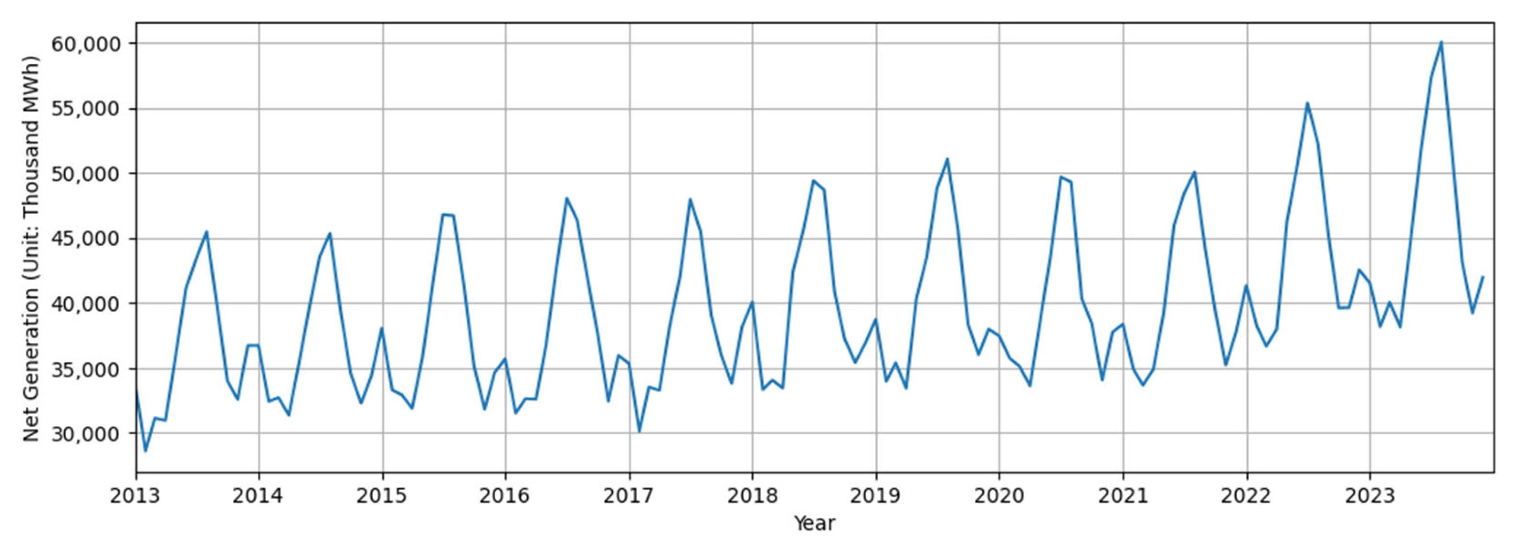
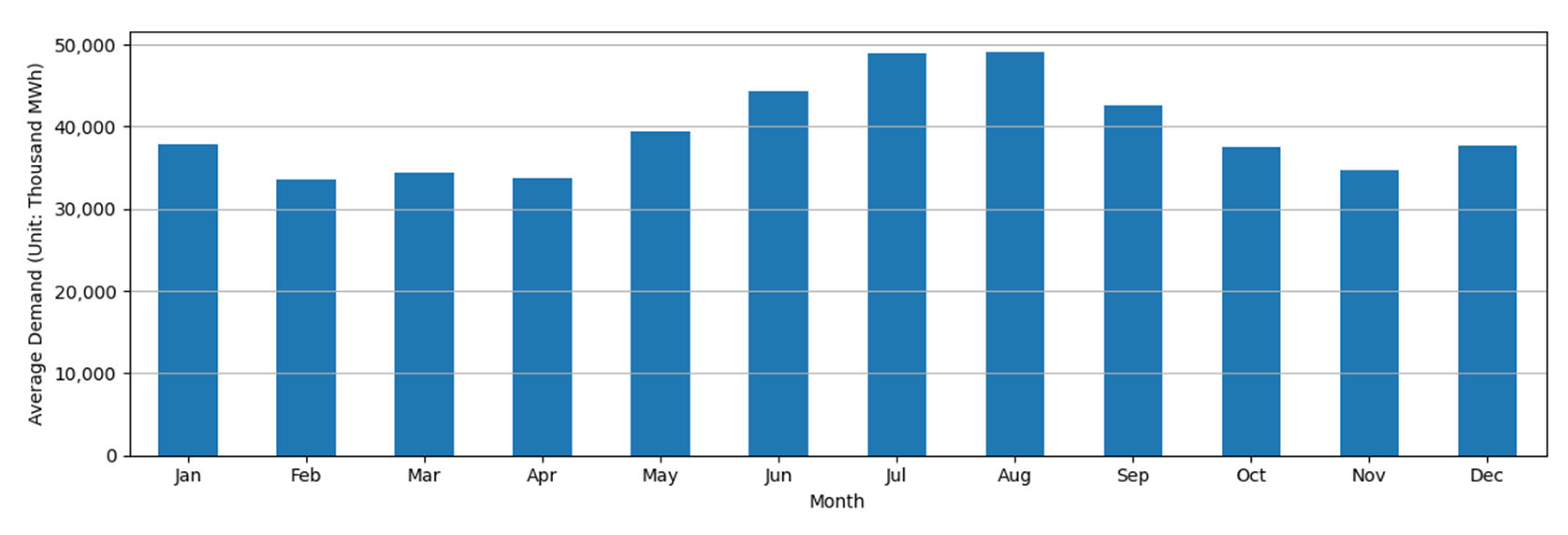
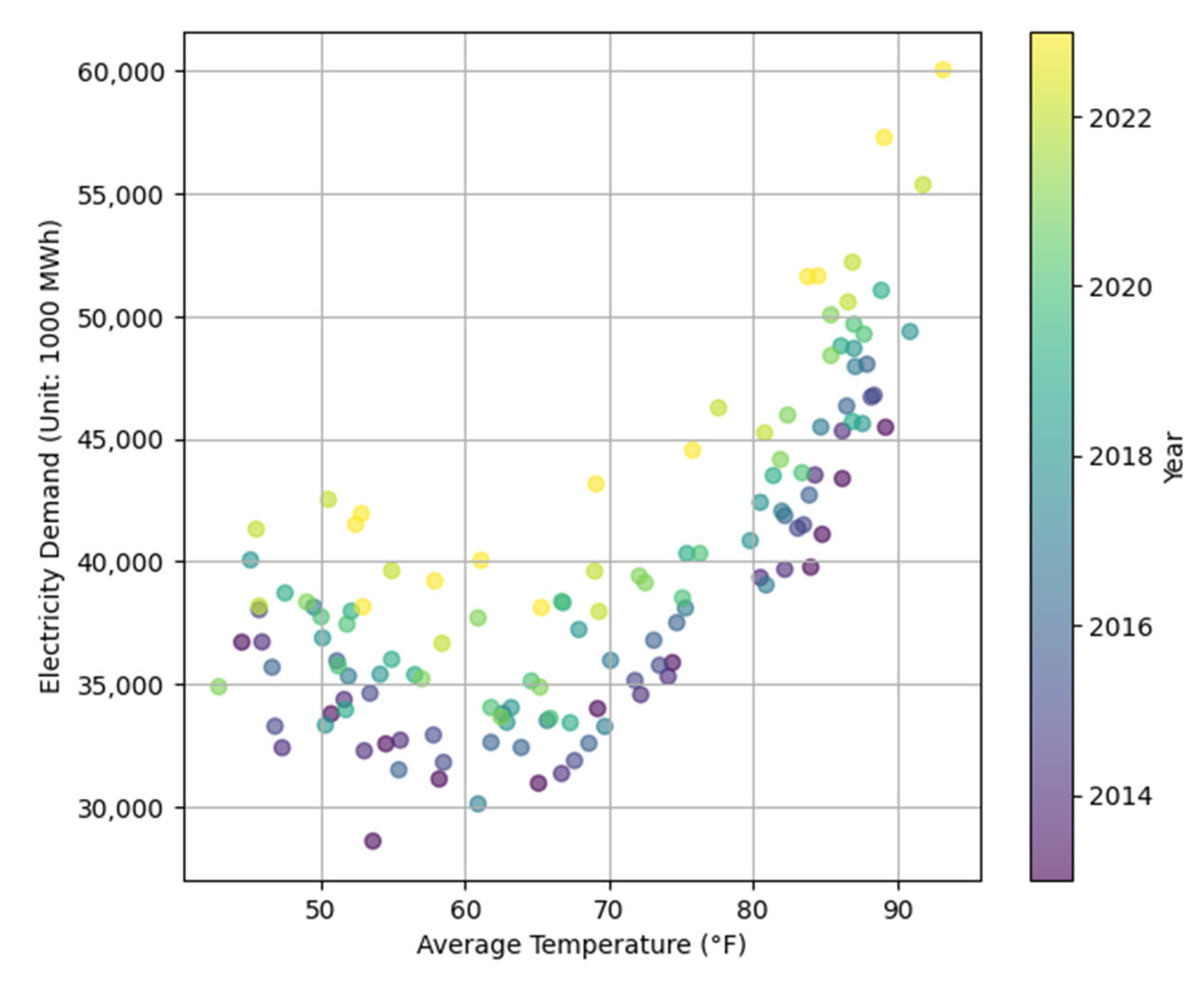
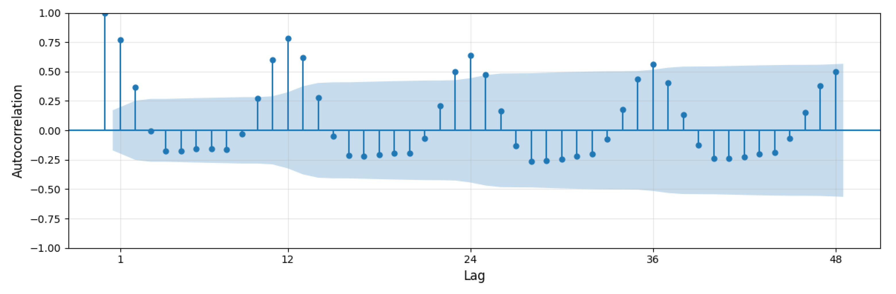
2. Data Analysis

To enhance the accuracy of electricity load forecasting, it is essential to first understand the characteristics of electricity demand in the Texas region from multiple perspectives. This section also explores various factors affecting the Texas grid to identify exogenous variables that influence its electricity demand. By analyzing these characteristics, we seek to provide meaningful insights that can improve the design of the forecasting model. Net electricity generation data for Texas were collected from the U.S. Energy Information Administration (EIA) via its public data portal (https://www.eia.gov/electricity/data/browser/#/topic/0?agg=1,0,2&fuel=g&geo=0000000002&sec=o3g&freq=M&start=200101&end=202505&ctype=linechart&ltype=pin&rtype=s&pin=&rse=0&maptype=0 accessed on 1 April 2025) and used to represent electricity demand. Figure 1 shows a time series plot (in 1000 MWh) of monthly electricity demand in Texas from 2013 to 2023.

As you can see from Figure 1, several key temporal characteristics of the time series are revealed. First, the demand exhibits a modest upward trend over the ten-year span. Notably, after 2020, the overall demand level seems to increase more markedly. Also, a strong seasonal pattern is observed, with electricity demand repeatedly peaking during the summer months as well as relatively small peaks during the winter months. Lastly, increasing volatility is observed in recent years (2021–2023), with greater amplitude observed in monthly demand variations. This trend may reflect growing complexity in the Texas electricity system, driven by factors such as weather anomalies, grid constraints, and rising electricity demand from non-traditional sources like AI-driven data centers. These characteristics address the need for forecasting models that can effectively accommodate an upward trend, seasonality, and increasing volatility.

To more clearly capture the seasonal characteristics of electricity demand in Texas, Figure 2 shows the monthly average electricity consumption for each calendar month from 2013 to 2023. As shown in the figure, electricity demand varies significantly throughout the year, confirming the presence of strong intra-annual seasonality. The highest average demand occurs during the summer months, i.e., July and August. This seasonal peak is largely attributable to increased use of air conditioning during hot summers. During the winter season, electricity demand tends to rise in January and December; however, the magnitude of demand in these months remains lower than that observed in June and September. This indicates that while heating needs may contribute to increased consumption during colder months, their impact is less pronounced than the cooling-driven spikes observed in the summer. The following figure shows the relationship between electricity demand and average temperature in a representative region of Texas.

Figure 3 displays a scatter plot illustrating the relationship between monthly electricity demand and average temperature in Texas. Each point represents a single month from 2013 to 2023, and the color gradient indicates the corresponding year, with darker tones representing earlier years and lighter tones representing more recent years. Temperature data are based on monthly averages from Dallas—the most populous city in Texas—and were obtained from the website of the National Weather Service (https://www.weather.gov/wrh/climate accessed on 1 April 2025). The plot reveals a distinct convex nonlinear relationship between average temperature and electricity demand. Specifically, electricity consumption tends to be relatively moderate in the mid-temperature range, while it increases at both ends of the temperature scale. This also suggests that when temperatures are either very high or very low, their effects on electricity demand become amplified. Given this amplification, it is worth considering the inclusion of a squared temperature term as an explanatory variable in the forecasting model.

Figure 4 presents the autocorrelation function (ACF) plot of monthly electricity demand in Texas, providing insights into the temporal dependence structure of the time series. As observed in the figure, electricity demand exhibits strong autocorrelation at lag 1 and significant spikes in autocorrelation are evident at 12-month intervals, suggesting the presence of annual seasonality in the data. These findings imply that past values—particularly those from the same month in the previous year—contain valuable predictive information. Therefore, incorporating lagged features is likely essential for improving the accuracy of monthly load forecasting models.

Thus far, we have confirmed typical characteristics of monthly electricity demand, including upward trends, seasonal fluctuations, autocorrelations, and their relationship with temperature. As a final component of this section, we turn our attention to the geo-economic context of Texas. As noted earlier, Texas has emerged as one of the most active regions for data center construction. In addition to digital infrastructure, the state continues to attract a diverse array of businesses, electrify oil and gas operations, and so on. These changes have collectively led to a sharp increase in industrial electricity demand [23]. The following figure presents a visualization that allows for indirect observation of the relationship between industrial activity and electricity demand.

To indirectly capture the intensity of industrial activity in Texas, this study first considers the number of weekday holidays in each month as a proxy indicator. Figure 5 presents the relationship between the number of weekday holidays in a given month (as defined by federal and Texas state holidays) and average electricity demand. As the number of weekday holidays increases, a general decline in electricity consumption is observed. This inverse relationship supports the hypothesis that reduced working days are associated with lower levels of industrial and commercial electricity usage. These results indicate that calendar-based variables can serve as meaningful proxies for industrial activity and need to be incorporated into the forecasting model.

3. Methodology

This study proposes a regression-based framework for forecasting monthly electricity demand in the Texas region. The predictive performance of such a model is heavily dependent on the selection and construction of input variables. As discussed in the previous section, Texas’s electricity demand exhibits distinct temporal patterns—such as trend, seasonality, and autocorrelation—as well as sensitivity to exogenous factors including temperature and industrial activity. Therefore, effectively translating these influences into well-structured input variables is essential for enhancing model accuracy. Although regression is a traditional forecasting approach, when properly designed with domain-specific variables, it can outperform more complex machine learning techniques. This section is organized as follows: Section 3.1 outlines the input variables used in the model, Section 3.2 introduces the proposed regression model, and Section 3.3 presents the forecasting procedure using the proposed model.

3.1. Input Variables

3.1.1. Trend

A common approach to capturing trend effects in time series forecasting models is to include a time index as an input variable. Since this study focuses on monthly data, the time index t is defined such that January 2013 (the beginning of the training period) corresponds to t = 1, and increases by one each month, reaching t = 132 in December 2023. Including this index as a variable in the model allows for the representation of linear trends in electricity demand.

However, as observed in Figure 1, electricity demand in Texas has exhibited an accelerating upward trend in recent years, particularly driven by the expansion of data centers and industrial activity. This pattern suggests that a nonlinear trend specification is more appropriate. To account for acceleration, we include a squared time index term (t²) as an input variable. By doing so, this study indirectly accounts for the accelerating electricity demand driven by data center expansion or industrial growth.

3.1.2. Autocorrelations

As identified in the ACF plot shown in Figure 4, monthly electricity demand in Texas exhibits strong temporal dependence, particularly with the immediately preceding month and the same month of the previous year. To reflect this autocorrelation structure, the forecasting model should include lagged demand variables as predictors. Let y_t denote the electricity demand at time t, which serves as the dependent variable in our model. To capture autocorrelative effects, the values of y_t−1 and y_t−12 would be considered as relevant input variables. However, in the context of monthly forecasting, incorporating the immediately preceding month’s demand (y_t−1) may not be feasible or appropriate, as future values are predicted multiple months ahead. As an alternative, this study adopts y_t−13, the electricity demand from the month prior to the same month last year, as a substitute variable. This lag still retains meaningful predictive power, as evidenced by its statistically significant autocorrelation in Figure 4.

3.1.3. Seasonality

Incorporating lagged demand from the same month of the previous year (i.e., y_t−12) reflects the autocorrelation, as mentioned earlier, but also partially captures seasonal effects. However, to explicitly represent seasonality, this study also includes a month indicator variable as an additional input feature. Let m_t denote the month corresponding to time t. There are generally two approaches to including this variable in a model. The first is to treat m_t as a categorical variable, where, for example, January 2013 would be encoded as “January” and December 2023 as “December.” While this approach accurately represents monthly seasonality, it requires the use of 11 dummy variables to encode 12 months, which increases model complexity and may lead to sparsity issues. Alternatively, the month variable can be treated as a numerical variable, where January is coded as 1, February as 2, …, and December as 12. Although this encoding assumes a linear ordering of months, empirical studies and practical applications often show that this simplification yields similar performance to categorical encoding.

This study proposes a new formulation of the month variable, to leverage the strengths of both approaches while mitigating their respective limitations. Specifically, instead of encoding months in calendar order (i.e., January = 1, …, December = 12), we assign numeric values to months based on their average electricity demand, as observed in train data. This approach retains the computational simplicity of a numeric variable, while embedding domain-relevant seasonal information directly into the feature. Figure 6 illustrates the average electricity demand for each calendar month from 2013 to 2023, sorted in ascending order.

In this study, we assign the modified month variable according to the ascending order of average monthly electricity demand, as shown in Figure 6. For example, February is assigned a value of 1, April is assigned 2, and August is assigned a value of 12. In summary, the modified month variable takes the values 7, 1, 3, 2, 8, 10, 11, 12, 9, 5, 4, and 6 for the month indices corresponding to January, February, …, December, respectively. This reordering embeds the demand intensity of each month into a single numeric variable, allowing the model to better capture seasonal variation while avoiding the dimensionality inflation associated with dummy encoding

3.1.4. Temperature

As observed in Figure 3, there exists a clear nonlinear relationship between electricity demand and temperature in Texas. To capture this effect, it is essential to include temperature variables in the model. However, a challenge arises from the geographical diversity of the state—temperature varies across different regions. The National Weather Service provides monthly average temperature data for major Texas regions, including Dallas, Houston, Austin, and San Antonio. To determine the most representative temperature input for the model, this study first computes the Pearson correlation coefficients between monthly electricity demand and the average temperatures of each city. In addition, we calculate the correlation between electricity demand and the average of the four cities’ temperatures, treating it as a potential aggregate indicator. The results are summarized in

Table 2. Correlation coefficient values between monthly electricity demand and average monthly temperature in different regions in Texas.

Cities	Dallas	Houston	Austin	San Antonio	Average
Correlation Coefficients	0.715	0.707	0.714	0.702	0.711

below.

As shown in Table 2, all four cities exhibit strong positive correlations between monthly electricity demand and average temperature. Among them, Dallas has the highest correlation coefficient, suggesting that temperature fluctuations in Dallas are most closely aligned with variations in statewide electricity demand. This may be attributed to Dallas being the most populous city in Texas and a central hub for data center development, both of which significantly influence total electricity usage. Based on these results, this study selected the average monthly temperature of Dallas as the representative temperature variable in the proposed forecasting model.

Additionally, to examine whether extremely high or low temperatures have an amplified effect on electricity demand, we computed the correlation between the squared term of Dallas’s average monthly temperature and electricity demand. The resulting correlation coefficient was 0.755, which is notably higher than the 0.715 obtained for the linear temperature term. This finding supports the hypothesis that nonlinear effects of temperature are significant and, thus, the squared temperature variable was also selected in the forecasting model.

3.1.5. Other Features

As the final case of input variables, this study includes a calendar-based feature introduced in the previous section: the number of weekday holidays. Let h_t represent the number of weekday holidays in the same month. This variable is intended to serve as proxies for industrial activity, which is a key driver of electricity demand. While it is theoretically possible to incorporate direct measures of industrial output or sector-specific electricity consumption, doing so poses several challenges—most notably, limited data availability and the impracticality of knowing future values for predictive purposes. In contrast, h_t is deterministic calendar attributes that can be easily known in advance for any future time point, making them especially suitable for forecasting tasks. By incorporating this variable, the proposed model can reflect the expected monthly variation in electricity demand driven by the operational intensity of industrial and commercial sectors.

3.2. Proposed Regression Model

Building upon the input features discussed in the previous subsection, this study proposes a multiple linear regression model to forecast monthly electricity demand in Texas. The model aims to capture both temporal and exogenous influences using a structured and interpretable set of input variables. The functional form of the proposed regression model, which regresses monthly electricity demand y_t, is expressed as

$$y_t = {\beta }_0 + {\beta }_1{t}^2 + {\beta }_2{y}_{t-12} + {\beta }_3{y}_{t-13} + {\beta }_4{m}_t + {\beta }_5{T}_t + {\beta }_6{T}_t^2 + {\beta }_7{h}_t+{\beta }_8(T_t\cdot m_t) + {ϵ}_t,$$

(1)

where

t is the time index representing the upward trend of the monthly electricity demand;

y_t−12 is the electricity demand from the same month in the previous year of the t-th month;

y_t−13 is the electricity demand from the month prior to the same month last year of the t-th month;

m_t is the modified month variable at the t-th month such that if the months of the t-th months are January, February, March, April, May, June, July, August, September, October, November, and December, then the m_t are 7, 1, 3, 2, 8, 10, 11, 12, 9, 5, 4, and 6, respectively;

T_t is the average monthly temperature in Dallas at the t-th month;

h_t is the number of weekday holidays at the t-th month;

β_i represents the coefficient of i-th term of the model, for i = 1, 2, …, 8;

and ϵ_t denotes the error term.

All terms from the first to the seventh in the proposed model (i.e., β₁t² to β₇h_t) directly correspond to the input variables introduced in Section 3.1, so it is not hard to understand. However, the final term, the interaction between average temperature and the modified month (β₈(T_t⋅m_t)), might need additional explanation. As shown in Figure 3, electricity demand increases not only at high temperatures but also at low temperatures, indicating a U-shaped relationship. To capture this effect, the model introduces an interaction term between temperature and the month. Consequently, this formulation offers interpretability, computational simplicity, and flexibility in capturing key structural patterns of the demand. The adjusted R² value of the proposed model is 0.966 when fitting the model on train data, which indicates that the proposed model has a sufficient goodness of fit. To assess the statistical significance of each term included in the model, the regression coefficients summary is presented below.

Table 3. Estimated coefficients and significance levels in the proposed model.

Variables	Coefficients	Standard Errors	t-Statistics	p-Values
Intercept	73,680	4868.246	15.135	<0.001
t2	0.3235	0.024	13.548	<0.001
yt−12	0.1672	0.065	2.587	0.011
yt−13	0.0038	0.029	0.131	0.896
mt	961.6119	279.012	3.446	0.001
Tt	−1683.94	142.579	−11.811	<0.001
$T_t^2$	14.2224	1.304	10.903	<0.001
ht	−104.056	145.193	−0.717	0.475
Tt⋅mt	−9.0074	4.744	−1.898	0.060

summarizes the estimated regression coefficients and associated statistical metrics for the proposed model. Several key findings emerge from this table regarding the contribution and statistical significance of individual predictors. The quadratic time trend variable t² shows a highly significant positive coefficient, confirming the presence of an accelerating upward trend in electricity demand over time. The lagged demand from the same month in the previous year is also statistically significant, indicating a strong seasonal autocorrelation effect. In contrast, the additional lag variable does not reach conventional levels of significance, suggesting its marginal predictive value may be limited when y_t−12 is already included in the model. The modified month variable designed to capture seasonality has a highly significant positive effect. This demonstrates that embedding seasonal intensity directly into the month encoding provides useful information for demand prediction. The temperature variable, both in its linear and squared forms, appears to be highly significant, indicating its critical role in forecasting monthly electricity demand in Texas. Its inclusion in the interaction term further reinforces its importance, suggesting that temperature is the most influential input variable in the proposed model. The calendar variable, h_t, does not show statistical significance; however, we retain this variable in the model to account for industrial activity. Overall, the regression results confirm that most of the proposed input variables contribute meaningfully to model performance, and the inclusion of nonlinear and interaction effects enhances the model’s ability to capture structural characteristics of electricity demand in Texas.

In this study, to empirically assess the contribution of the key variables, i.e., the squared time index, squared temperature, the modified month variable, and the interaction term between temperature and month, we conducted a comparative model evaluation. The goal is to determine how much these specially designed variables improve model fit compared to more conventional alternatives or models excluding these terms.

Table 4. Model fitness of the proposed and comparative regression models.

Models		Adj. R2
Proposed Model	yt = β0$+ {\beta }_1{t}^2 + {\beta }_2{y}_{t-12} + {\beta }_3{y}_{t-13} + {\beta }_4{m}_t + {\beta }_5{T}_t + {\beta }_6{T}_t^2$ + β7ht + β8(Tt⋅mt) + ϵt	0.966
Comparative Models	yt = β0$+ {\beta }_{1}t + {\beta }_2{y}_{t-12} + {\beta }_3{y}_{t-13} + {\beta }_4{m}_t + {\beta }_5{T}_t + {\beta }_6{T}_t^2$ + β7ht + β8(Tt⋅mt) + ϵt	0.959
	yt = β0 + β1t2 + β2yt−12 + β3yt−13 + β4mt + β5Tt + β6ht + β7(Tt⋅mt) + ϵt	0.933
	yt = β0$+ {\beta }_1{t}^2 + {\beta }_2{y}_{t-12} + {\beta }_3{y}_{t-13} + {\beta }_4{o}_t + {\beta }_5{T}_t + {\beta }_6{T}_t^2$dt + β7ht + β8(Tt⋅ot) + ϵt	0.959
	yt = β0$+ {\beta }_1{t}^2 + {\beta }_2{y}_{t-12} + {\beta }_3{y}_{t-13} + {\beta }_4{m}_t + {\beta }_5{T}_t + {\beta }_6{T}_t^2$dt + β7ht + ϵt	0.965

summarizes the adjusted R² values of the proposed regression model and four comparative models, each differing slightly in their specification of explanatory variables. The proposed model achieves the highest adjusted R², which indicates the strongest explanatory power among the tested specifications. The alternative models are designed to assess the contribution of individual components by selectively excluding or modifying certain variables. For instance, replacing the nonlinear time trend (t²) with a linear time trend (t) reduces the adjusted R² to 0.959. Omitting the squared temperature term ($T_t^2$) leads to the greatest decrease in the model fit, reducing the adjusted R² to 0.933. Models using the ordinary numerical month variable (o_t) instead of m_t or excluding the interaction term perform slightly worse than the proposed model. These results confirm that the inclusion of nonlinear and interaction terms, especially the squared temperature variable, meaningfully enhances the model’s explanatory capability.

Particularly, the modified month variable (m_t) is a new feature proposed in this study. To further justify its use over traditional monthly representations, we provide an additional comparative analysis with the conventional month variables in Appendix A.1. Additionally, Appendix A.2 presents a supplementary comparative experiment focusing on the interaction between the month variable and temperature. In this study, we use the interaction term to reflect that the effect of temperature on electricity demand may vary by season. However, conventional approaches typically use heating degree days (HDDs) and cooling degree days (CDDs) to capture this nonlinear response [24]. To validate the effectiveness of our approach, we compare it against a model utilizing HDD and CDD variables.

3.3. Forecasting Procedure with the Proposed Model

This subsection outlines the step-by-step procedure used to implement the proposed regression-based forecasting model. The forecasting process involves model training on historical data and subsequent application to generate out-of-sample predictions. In this study, we adopt a rolling forecasting approach, conducting separate 12-month-ahead forecasts for both 2023 and 2024. Accordingly, the following procedure is executed twice, once immediately before each forecast year. The detailed steps are as follows:

• Step 0. Specify the Forecasting and Training Periods
  • We first designate the forecasting period, and then set the training period as the time span from January 2013 up to the immediately preceding month of the forecasting year. Specifically, the training data consists of monthly observations from January 2013 to December 2022 when forecasting 2023, and from January 2013 to December 2023 when forecasting 2024, respectively.
• Step 1. Collect Data for the Training Period
  • For the training data, we gather all input variables and the dependent variable from the designated training period. In this study, for each month within the training period, we collect or calculate the following data: the electricity demand for that month, the electricity demand from 12 and 13 months prior, the average monthly temperature in Dallas, the time index, and the modified month variable.
• Step 2. Fit the Proposed Regression Model
  • Using the collected training data, we estimate the coefficients of the proposed multiple linear regression model. The fitted model provides a closed-form regression equation with estimated parameters.
• Step 3. Collect Data for the Forecasting Period
  • We collect the same set of input variables for the forecasting period. Since this study performs 12-month-ahead forecasting, all input variable data for the entire forecasting year must be gathered in advance.
• Step 4. Generate Forecasts Using the Regression Equation
  • The regression equation from Step 2 is applied to the input variable values collected in Step 3 to compute the forecasts for the forecasting period.
• Step 5. Evaluate Forecast Accuracy
  • The forecast values are compared with the actual values in the forecasting period, if available, to assess the accuracy of the model. Forecasting performance can be evaluated using well-known error metrics.

In this study, the above procedure is applied in a rolling manner to generate 12-month-ahead forecasts for both 2023 and 2024. Forecast accuracy is assessed for each forecasting year, and the results are presented in the next section. This includes comparative experiments with various benchmark models to validate the effectiveness of the proposed approach.

4. Computational Experiments

To evaluate the forecasting performance of the proposed regression model, a series of comparative experiments are conducted against several existing methods. The model is trained on monthly electricity demand data from 2013 up to the year preceding each forecast period. Following a rolling forecasting approach, we generate 12-month-ahead forecasts for both 2023 and 2024, resulting in two sets of out-of-sample predictions. Forecasts are then obtained for the 24 months of 2023 and 2024 using the forecasting procedure presented in Section 3.3, and the accuracy of these forecasts is assessed using three widely used metrics: Mean Absolute Error (MAE), Root Mean Square Error (RMSE), and Mean Absolute Percentage Error (MAPE). The mathematical definitions of the evaluation metrics are given as follows:

$$MAE={\sum }_{t=121}^n\left(\left|A_t-F_t\right|\right)/24$$

(2)

$$RMSE=\sqrt{{\sum }_{t=121}^n{\left(A_t-F_t\right)}^2/24}$$

(3)

$$MAPE=\left\{{\sum }_{t=121}^n\left({\displaystyle \frac{\left|A_t-F_t\right|}{A_t}}\right)/24\right\}\times 100\%,$$

(4)

where $A_t$ represents the actual value at the t-th month, $F_t$ denotes the forecasted value at the t-th month, n is 144, i.e., the month index of December 2024, in this study.

To objectively evaluate the performance of the proposed model, we compared it with a diverse set of well-known forecasting methods, all trained on the same dataset. The benchmark models consist of three univariate time series methods, three neural network-based models, and three machine learning algorithms. First, among the univariate statistical methods, we employed Holt–Winters, a representative exponential smoothing method capturing level, trend, and seasonal components [25]; SARIMA (Seasonal AutoRegressive Integrated Moving Average), a widely used time series model that incorporates autoregressive, differencing, and moving average terms, along with seasonal components [26]; and Prophet, a decomposable model developed by Meta that combines trend, seasonality, and holiday effects [27].

Second, for neural network-based models, we include Recurrent Neural Network (RNN), which models sequential dependencies through recurrent connections and is suitable for temporal data [28]; Long Short-Term Memory (LSTM), a more advanced architecture that mitigates the vanishing gradient problem in RNNs and is particularly effective at capturing long-term dependencies in time series data [29]; and a Transformer-based model designed for time series forecasting. This model adapts the Transformer architecture [30] by utilizing only the encoder component, incorporating multi-head self-attention and positional encoding, and tailoring the output layer for univariate time series prediction. Since neural network-based methods exhibit stochastic behavior, the forecast results may vary across runs. Thus, we performed each experiment three times with different random seeds and used the average of the three forecast results as the final forecast.

Third, widely used machine learning methods are tested: Random Forest, an ensemble of decision trees that improves prediction accuracy by reducing variance [31]; LightGBM, a gradient boosting framework known for its computational efficiency [32]; and XGBoost, another powerful boosting algorithm that incorporates regularization and is widely used in time series and structured data forecasting tasks [33]. All three machine learning methods were trained using the same set of input features, which include t, y_t−12, y_t−13, T_t, and h_t, as used in the proposed model and the ordinary numerical month variable (o_t). In contrast, the neural network-based models were trained as univariate models, using only past electricity demand values and basic date-related inputs. Major hyperparameter settings for these machine learnings as well as the above neural network-based models are summarized in the table in Appendix B. These benchmark models are chosen to reflect a wide methodological spectrum, ranging from traditional time series analysis to advanced deep learning and machine learning approaches. The results of the computational experiments are summarized in

Table 5. Forecasting results for 2023 and 2024 using the proposed and benchmark methods.

Methods			MAE	RMSE	MAPE
Proposed Model			998.9	1423.6	2.05%
Benchmarks	Univariate Models	Holt–Winters	1678.4	2201.3	3.57%
		SARIMA	1754.4	2229.5	3.75%
		Prophet	1733.8	2212.1	3.65%
	Neural Networks	RNN	2012.1	2605.1	4.30%
		LSTM	2704.6	3305.3	5.89%
		Transformer	2485.2	3076.9	5.29%
	Machine Learning	Random Forest	2224.5	2944.8	4.64%
		LightGBM	2662.0	3394.7	5.40%
		XGBoost	2544.7	3181.0	5.38%

.

Table 5 presents the forecasting performance of the proposed regression model compared with nine benchmark methods. The proposed model achieves the lowest error across all three metrics, clearly outperforming both traditional statistical models and more complex machine learning and neural network approaches. The proposed model is the only method that shows three-digit MAE results; moreover, it is the only method that shows around 2% MAPE. Among the benchmark models, the univariate approaches perform relatively well. This suggests that for monthly electricity demand forecasting in Texas, reasonably accurate results can be obtained by capturing typical time series features such as trend and seasonality. In the neural network category, RNN shows better performance than LSTM and Transformer. Among the machine learning models, Random Forest yields the best performance. Although these models are effective in general-purpose regression tasks, they lag behind the proposed model, which suggests that their forecasting accuracy is highly sensitive to how input variables are selected and manipulated. Overall, the proposed regression model delivers superior accuracy due to its carefully engineered input variables, such as the squared temperature variable and the modified month variable tailored for the Texas region. The relatively poor performance of neural network and machine learning methods may be attributed to the limited size of the training dataset, which is insufficient for these models to demonstrate their full potential.

Although a direct comparison with ERCOT’s official forecasts would also be informative, it is not feasible due to differences in forecasting horizons and temporal resolution. ERCOT produces short-term, mid-term, and long-term load forecasts with horizons ranging from hours to years and at resolutions such as 5-minute or hourly intervals, which are not aligned with the monthly forecasting framework adopted in this study. Nevertheless, the forecasting performance of the proposed model can be indirectly compared to that of prior monthly electricity load forecasting studies through MAPE values. While a direct comparison is not possible due to differences in forecasting regions, horizons, etc., the studies introduced in Section 1 reported MAPE values of 2.31% [7], 4.29% [8], 2.18% [9], 4.37% [10], and 3.78% [11]. When compared to the 2.05% MAPE achieved by the proposed model, this also supports the fact that our approach offers competitive forecasting accuracy.

To further demonstrate the robustness of the proposed model’s forecasting performance, we conducted a more detailed analysis of the forecasting errors. For each method, 24 absolute percentage errors (APEs) were calculated to obtain MAPEs. We summarized key descriptive statistics of these APEs in

Table 6. Mean, median, standard deviation, and maximums of APEs generated by the tested methods.

Methods	Mean (i.e., MAPE)	Median	Standard Deviation	Maximum
Proposed Model	2.05%	1.28%	1.96%	5.54%
Holt–Winters	3.57%	2.76%	2.77%	12.04%
SARIMA	3.75%	3.24%	2.63%	9.02%
Prophet	3.65%	3.20%	2.59%	9.55%
RNN	4.30%	4.31%	3.09%	12.89%
LSTM	5.89%	5.11%	4.10%	17.89%
Transformer	5.29%	4.73%	3.44%	13.35%
Random Forest	4.64%	4.03%	3.62%	12.15%
LightGBM	5.40%	4.82%	3.54%	15.62%
XGBoost	5.38%	4.38%	3.77%	12.56%

.

Table 6 presents the descriptive statistics of the APEs for each tested method, including the mean (i.e., MAPE), median, standard deviation, and maximums of APEs across the 24 forecasted months. The proposed regression-based model records the lowest MAPE of 2.05%. The median of APEs of the proposed model is 1.28%, substantially lower than those of the other methods. This suggests that the model consistently delivers accurate forecasts in most months. Furthermore, the standard deviation of APEs is only 1.96%, the lowest among all methods, indicating that the proposed model yields more stable, less variable errors over time. Additionally, the maximum is only 5.54%, which is substantially lower than those of all other benchmark models. This reinforces the model’s robustness in avoiding large forecasting failures, even during potentially volatile months. Overall, the combination of low average error, narrow error distribution, and small worst-case error emphasizes the robust and reliable performance of the proposed approach. Furthermore, to assess the statistical significance of the proposed model’s forecasting performance, we conducted paired t-tests between the 24 APEs generated by the proposed model and those from each benchmark model. The results of these statistical tests are summarized in

Table 7. Results of paired t-tests between proposed model and benchmarks.

	Holt–Winters	SARIMA	Prophet	RNN	LSTM	Transformer	Random Forest	LightGBM	XGBoost
p-values	0.043 *	0.021 *	0.017 *	0.007 †	0.001 †	0.001 †	<0.001 †	<0.001 †	<0.001 †

* Statistically significant at a significance level of 0.05. ^† Statistically significant at a significance level of 0.01.

.

Table 7 presents the p-values from paired t-tests conducted between the 24 APEs of the proposed model and those of each benchmark. All comparisons are statistically significant at a significance level of 0.05. These results provide strong statistical evidence that the proposed regression-based model consistently outperforms benchmarks. Thus, the robustness of the model’s predictive accuracy is supported not only by performance metrics such as MAPE but also by a statistical significance test. To gain a more detailed understanding of the forecasting outcomes, a comparison plot of the actual and predicted monthly electricity demand for the 24 months is provided below.

Figure 7 displays a comparison of the monthly electricity demand forecasts for both 2023 and 2024 generated by the proposed regression model, Holt–Winters, RNN, and Random Forest, alongside the actual observed values. For clarity, only one representative method from each benchmark category, namely Holt–Winters for univariate models, RNN for neural networks, and Random Forest for machine learning, was selected for comparison, based on their relatively superior performance among their respective groups. As shown in the figure, the proposed model (red solid line) closely follows the actual demand (black solid line) across both years. While all models capture the overall seasonal patterns and month-to-month variations, the proposed model demonstrates a consistently closer alignment with actual demand values, indicating its superior forecasting accuracy.

5. Conclusions

This study conducted a comprehensive investigation into the monthly electricity load forecasting problem in the Texas region, which critically requires accurate demand predictions in response to the rapid expansion of data centers and industrial activities. Through exploratory data analysis, we identified key characteristics of Texas electricity demand, including an accelerating upward trend, strong seasonality, increasing volatility, and correlations with temperature and industrial factors. To address these features, we developed a regression-based forecasting framework that incorporates a carefully engineered set of input variables, including nonlinear trends, seasonal patterns, lagged demand, linear and nonlinear temperature effects, and calendar-based proxies for industrial activity. In the proposed model, the squared time index variable, the modified month variable, and the squared temperature variable play key roles in enhancing forecasting performance of the model. The proposed model was validated against a diverse array of benchmark methods including Holt–Winters, SARIMA, Prophet, RNN, LSTM, Transformer, Random Forest, LightGBM, and XGBoost. It demonstrated superior performance, achieving an MAPE of 2.05%, which is considerably lower than that of all benchmarks.

Future research may extend this study in several important directions. First, while this study incorporated general exogenous factors such as temperature and calendar variables, further improvement may come from identifying region-specific external drivers that specifically impact electricity demand in Texas, such as data center deployment intensity, industrial electrification trends, and population or economic growth metrics in high-demand corridors. Second, although this study focused on forecasting a one-year horizon, future research may explore longer forecast horizons ranging from two to five years, which are particularly relevant for long-term capacity planning and investment decisions. Lastly, an ensemble approach that combines the strengths of neural networks or machine learning algorithms with statistical models could offer a promising direction. These hybrid methods could leverage the interpretability and stability of traditional techniques alongside the flexibility and nonlinearity-capturing power of data-driven models, potentially yielding even higher accuracy and robustness in mid- to long-term electricity demand forecasting.

References

- Wang, H.; Alattas, K.A.; Mohammadzadeh, A.; Sabzalian, M.H.; Aly, A.A.; Mosavi, A. Comprehensive Review of Load Forecasting with Emphasis on Intelligent Computing Approaches. Energy Rep. 2022, 8, 13189–13198. [Google Scholar] [CrossRef]
- Kuster, C.; Rezgui, Y.; Mourshed, M. Electrical Load Forecasting Models: A Critical Systematic Review. Sustain. Cities Soc. 2017, 35, 257–270. [Google Scholar] [CrossRef]
- IEA. Energy and AI. World Energy Outlook Special Report, International Energy Agency. 2025. Available online: https://www.iea.org/reports/energy-and-ai (accessed on 1 May 2025).
- Shehabi, A.; Smith, S.J.; Hubbard, A.; Newkirk, A.; Lei, N.; Siddik, M.A.B.; Holecek, B.; Koomey, J.; Masanet, E.; Sartor, D. 2024 United States Data Center Energy Usage Report; Lawrence Berkeley National Laboratory: Berkeley, CA, USA, 2024; LBNL-2001637. [Google Scholar]
- Bolner, A. 5 Reasons Why a Dallas Data Center Still Makes Good Sense. Stream Data Centers Excecutive Brief. 23 March 2021. Available online: https://www.streamdatacenters.com/articles/markets/why-dallas/ (accessed on 20 May 2025).
- Khuntia, S.R.; Rueda, J.L.; van der Meijden, M.A.M.M. Forecasting the Load of Electrical Power Systems in Mid- and Long-Term Horizons: A Review. IET Gener. Transm. Distrib. 2016, 10, 3971–3977. [Google Scholar] [CrossRef]
- Sharma, A.; Jain, S.K. A Novel Two-Stage Framework for Mid-Term Electric Load Forecasting. IEEE Trans. Ind. Inform. 2024, 20, 247–255. [Google Scholar] [CrossRef]
- Rubasinghe, O.; Zhang, X.; Chau, T.K.; Chow, Y.H.; Fernando, T.; Iu, H.H.-C. A Novel Sequence to Sequence Data Modelling Based CNN-LSTM Algorithm for Three Years Ahead Monthly Peak Load Forecasting. IEEE Trans. Power Syst. 2024, 39, 1932–1947. [Google Scholar] [CrossRef]
- Li, J.; Lei, Y.; Yang, S. Mid-Long Term Load Forecasting Model Based on Support Vector Machine Optimized by Improved Sparrow Search Algorithm. Energy Rep. 2022, 8, 491–497. [Google Scholar] [CrossRef]
- Dudek, G.; Pełka, P. Pattern Similarity-Based Machine Learning Methods for Mid-Term Load Forecasting: A Comparative Study. Appl. Soft Comput. 2021, 104, 107223. [Google Scholar] [CrossRef]
- Oreshkin, B.N.; Dudek, G.; Pełka, P.; Turkina, E. N-BEATS Neural Network for Mid-Term Electricity Load Forecasting. Appl. Energy 2021, 293, 116918. [Google Scholar] [CrossRef]
- Popik, T.; Humphreys, R. The 2021 Texas Blackouts: Causes, Consequences, and Cures. J. Crit. Infrastruct. Policy 2021, 2, 47–73. [Google Scholar] [CrossRef]
- Ali, M. Electricity Load Forecasting in Texas Using Neural Networks to Enhance the Power Grid Stability. Master’s Dissertation, Texas Tech University, Lubbock, TX, USA, 2024. [Google Scholar]
- Derner, R.; Butler, R.; Neff, A.; Ruthford, A. Reevaluating Texas Energy Market Forecasts in The Wake of Recent Extreme Weather Events. SMU Data Sci. Rev. 2024, 8, 8. [Google Scholar]
- Eysenbach, J.; Franklin, B.; Larsen, A.; Lindsey, J. Predicting Power Using Time Series Analysis of Power Generation and Consumption in Texas. SMU Data Sci. Rev. 2021, 5, 5. [Google Scholar]
- Hossain, R. Machine Learning Tools in the Predictive Analysis of ERCOT Load Demand Data. Master’s Dissertation, The University of Texas Rio Grande Valley, Edinburg, TX, USA, 2022. [Google Scholar]
- Mostafa, T.; Fouda, M.M.; Abdo, M.G. Short-Term Load Forecasting Employing Recurrent Neural Networks. In Proceedings of the 2024 International Conference on Smart Applications, Communications and Networking (SmartNets), Washington, DC, USA, 28–30 May 2024; pp. 1–6. [Google Scholar]
- Rice, R.; North, K.; Hansen, G.; Pearson, D.; Schaer, O.; Sherman, T.; Vassallo, D. Time-Series Forecasting Energy Loads: A Case Study in Texas. In Proceedings of the 2022 Systems and Information Engineering Design Symposium (SIEDS), Charlottesville, VA, USA, 28–29 April 2022; pp. 196–201. [Google Scholar]
- Ruthford, A.; Sadler, B. Modeling Electric Energy Generation in ERCOT during Extreme Weather Events and the Impact Renewable Energy Has on Grid Reliability. SMU Data Sci. Rev. 2021, 5, 6. [Google Scholar]
- Singh, G. Comparative Analysis of Machine Learning Models for ERCOT Short Term Load Forecasting. Master’s Dissertation, Virginia Tech, Blacksburg, VA, USA, 2025. [Google Scholar]
- Yang, J.; Tuo, M.; Lu, J.; Li, X. Analysis of Weather and Time Features in Machine Learning-Aided ERCOT Load Forecasting. In Proceedings of the 2024 IEEE Texas Power and Energy Conference (TPEC), College Station, TX, USA, 12–13 February 2024; pp. 1–6. [Google Scholar]
- NKF Research. Data Center Market Overview: Second Half 2019; Newmark Knight Frank: New York, NY, USA, 2019. [Google Scholar]
- LCG Consulting. 2025 ERCOT Electricity Market Outlook. August 2024. Available online: https://www.energyonline.com/reports/2025_ERCOT_Outlook.pdf (accessed on 5 June 2025).
- Skiles, M.J.; Rhodes, J.D.; Webber, M.E. Perspectives on Peak Demand: How Is ERCOT Peak Electric Load Evolving in the Context of Changing Weather and Heating Electrification? Electr. J. 2023, 36, 107254. [Google Scholar] [CrossRef]
- Winters, P.R. Forecasting Sales by Exponentially Weighted Moving Averages. Manag. Sci. 1960, 6, 324–342. [Google Scholar] [CrossRef]
- Box, G.E.P.; Jenkins, G.M.; Reinsel, G.C. Time Series Analysis Forecasting and Control, 4th ed.; John Wiley and Sons: Hoboken, NJ, USA, 2008. [Google Scholar]
- Taylor, S.J.; Letham, B. Forecasting at Scale. PeerJ, 2017; preprint. [Google Scholar] [CrossRef]
- Rumelhart, D.E.; Hinton, G.E.; Williams, R.J. Learning Representations by Back-Propagating Errors. Nature 1986, 323, 533–536. [Google Scholar] [CrossRef]
- Hochreiter, S.; Schmidhuber, J. Long Short-Term Memory. Neural Comput. 1997, 9, 1735–1780. [Google Scholar] [CrossRef] [PubMed]
- Vaswani, A.; Shazeer, N.; Parmar, N.; Uszkoreit, J.; Jones, L.; Gomez, A.N.; Kaiser, L.; Polosukhin, I. Attention Is All You Need. arXiv 2023, arXiv:1706.03762. [Google Scholar] [CrossRef] [PubMed]
- Breiman, L. Random Forests. Mach. Learn. 2001, 45, 5–32. [Google Scholar] [CrossRef]
- Ke, G.; Meng, Q.; Finley, T.; Wang, T.; Chen, W.; Ma, W.; Ye, Q.; Liu, T.-Y. LightGBM: A Highly Efficient Gradient Boosting Decision Tree. In Advances in Neural Information Processing Systems; Curran Associates, Inc.: Red Hook, NY, USA, 2017; Volume 30. [Google Scholar]
- Chen, T.; Guestrin, C. XGBoost: A Scalable Tree Boosting System. In Proceedings of the 22nd ACM SIGKDD International Conference on Knowledge Discovery and Data Mining, KDD’16, San Francisco, CA, USA, 13–17 August 2016; Association for Computing Machinery: New York, NY, USA, 2016; pp. 785–794. [Google Scholar]
- Schwarz, G. Estimating the Dimension of a Model. Ann. Stat. 1978, 6, 461–464. [Google Scholar] [CrossRef]