Article

Methods for Measuring and Computing the Reference Temperature in Newton’s Law of Cooling for External Flows

1
School of Aeronautics and Astronautics, Purdue University, West Lafayette, IN 47907, USA
2
Ames National Laboratory, U.S. Department of Energy, Ames, IA 50011, USA
3
National Energy Technology Laboratory, U.S. Department of Energy, Pittsburgh, PA 15236, USA
*
Author to whom correspondence should be addressed.
Energies 2025, 18(15), 4074; https://doi.org/10.3390/en18154074 (registering DOI)
Submission received: 29 June 2025 / Revised: 13 July 2025 / Accepted: 28 July 2025 / Published: 31 July 2025

Abstract

Newton’s law of cooling requires a reference temperature ( T r e f ) to define the heat-transfer coefficient ( h ). For external flows with multiple temperatures in the freestream, obtaining T r e f is a challenge. One widely used method, referred to as the adiabatic-wall (AW) method, obtains T r e f by requiring the surface of the solid exposed to convective heat transfer to be adiabatic. Another widely used method, referred to as the linear-extrapolation (LE) method, obtains T r e f by measuring/computing the heat flux ( q s ) on the solid surface at two different surface temperatures ( T s ) and then linearly extrapolating to q s = 0 . A third recently developed method, referred to as the state-space (SS) method, obtains T r e f by probing the temperature space between the highest and lowest in the flow to account for the effects of T s or q s on T r e f . This study examines the foundation and accuracy of these methods via a test problem involving film cooling of a flat plate where q s switches signs on the plate’s surface. Results obtained show that only the SS method could guarantee a unique and physically meaningful T r e f where T s = T r e f on a nonadiabatic surface q s = 0 . The AW and LE methods both assume T r e f to be independent of T s , which the SS method shows to be incorrect. Though this study also showed the adiabatic-wall temperature, T A W , to be a good approximation of T r e f (<10% relative error), huge errors can occur in h about the solid surface where | T s T A W | is near zero because where T s = T A W , q s 0 .

1. Introduction

Convective heat transfer, q s , at any location on a solid surface, such as the one shown in Figure 1, is typically characterized by the heat-transfer coefficient, h , defined by Newton’s law of cooling [1]:
q s = h ( T s T r e f )
In the above equation, T s is the temperature on the surface at the location of q s , and T r e f is the reference temperature corresponding to that location. T r e f represents the effective temperature in the fluid that drives the heat transfer either to or from the solid surface. Based on Equation (1), q s should equal zero where T s = T r e f .
For external flows, the adiabatic-wall temperature, T A W (also known as the recovery temperature), has traditionally been used as the T r e f [2,3,4]. The adiabatic-wall temperature is the temperature distribution on the solid’s surface where q s = 0 at all locations on the surface. Thus, when computational fluid dynamics (CFD) is used to obtain T A W , the adiabatic-wall boundary condition is imposed on all solid surfaces [3,4]. Similarly, experimental studies that seek to measure T A W have used insulators as solids to approximate an adiabatic wall [2,5]. When T A W is used as T r e f in Equation (1) on a non-adiabatic wall, the h obtained is denoted as h A W . The method that uses the adiabatic-wall temperature as T r e f is referred to as the adiabatic-wall (AW) method. With the AW method, T r e f is assumed to be independent of the T s and the corresponding q s on the non-adiabatic wall of the problem studied since neither T s or q s was used to compute T A W .
Since an adiabatic wall is difficult to produce in the laboratory, many studies obtain T r e f by measuring T s and q s on the non-adiabatic wall of the problem studied at two different thermal conditions, namely, ( T s 1 , q s 2 ) and ( T s 1 , q s 2 ) —and then linearly extrapolating to q s = 0   [6,7,8,9,10,11] to obtain the reference temperature; i.e.,
T s 1 T r e f , L E T s 1 T s 2 = q s 1 0 q s 1 q s 2       or       q s 1 q s 2 T s 1 T s 2 = q s 1 T s 1 T r e f , L E = q s 2 T s 2 T r e f , L E = h L E
The T r e f and h obtained by this method, referred to as the linear-extrapolation (LE) method, are denoted as T r e f , L E and h L E and are given by
T r e f , L E = ( q s , 2 T s 1 q s , 1 T s 2 ) / ( T s , 2 T s , 1 )
h L E = ( q s , 2 q s , 1 ) / ( T s , 2 T s , 1 )
Thus, the LE method assumes T r e f and h to depend only on the ratio of ( q s , 2 T s 1 q s , 1 T s 2 ) to ( T s i T s j ) and ( q s i q s j ) to ( T s i T s j ), respectively, and independent of the actual temperature or heat flux on the non-adiabatic wall of the problem studied. Basically, any pair of ( T s ,   q s ) could be used. Since there are uncertainties in experimental measurements, more than one pair of ( T s ,   q s ) is measured, and a straight line based on linear least-squares fit is used to obtain T r e f , L E and h L E .
Unlike the AW method, the challenge in implementing the LE method affects both computational and experimental methods. This is because it is unclear how the thermal condition on the solid surface should be changed to produce two pairs of ( T s ,   q s ) needed to obtain T r e f , L E and h L E and not change the actual problem being studied since the actual problem studied only has one set of T s and corresponding q s distribution, not two or more. Furthermore, the assumption that h is independent of   T s and   q s , which forms the basis of the LE method, is not supported by past studies. References [12,13,14,15,16,17,18,19] show h to have dependence on T s when there are appreciable density and/or transport property variations in the boundary layer, which on temperature. For example, Fitt et al. [18] suggested a correction to h involving the ratio of T A W to T s . Others use ratios of the viscosity at T A W to T s [1].
Moffat and co-workers [19,20,21,22,23], Hacker & Eaton [24], and He [25] examined heat flux on surfaces of non-adiabatic walls with arbitrary temperature distributions by using discrete, inverse, and continuous Green’s functions. In their studies, they showed upstream heat transfer to strongly affect downstream heat transfer, which implies T r e f to depend on T s and the corresponding q s .
Since conduction heat transfer in solids is orders of magnitude slower than convective heat transfer in gases, implementation of AW and LE methods can be time-consuming for heat-transfer problems that are steady. Thus, transient methods are often used to speed up the experimental procedure. With transient methods, T r e f and h in Equation (1) are obtained by using the exact solution of the one-dimensional, unsteady conduction in a semi-infinite solid that is initially at a uniform temperature of T i = T s ( t = 0 ) and at time t = 0 is suddenly exposed to a convective environment characterized by T r e f and h . That exact solution is given by [26,27]
T s ( t ) T i T r e f T i = 1 exp h 2 α   t k s 2 erfc h α t k s
where k s and α are the thermal conductivity and the thermal diffusivity of the solid, and they are constants. With Equation (5), computing or measuring the temperature on the solid surface, T s ( t ) , at two instances of time, t 1 and t 2 , yields two equations to obtain the two unknowns: T r e f and h . Since T s at any time t could be used, this method also assumes T r e f and h are independent of the actual T s and   q s on the non-adiabatic wall of the problem studied. Though many have used this method (see, e.g., Refs. [28,29,30,31,32,33,34,35,36,37,38]) and efforts have been made to correct and assess errors created by the assumption of one-dimensional heat transfer [39,40,41], Sathyanarayanan & Shih [42] showed that this method could create huge errors if the nature of the flow changes significantly in time once the thermal boundary layer grows from the initially uniform temperature in the solid and fluid. Thus, they do not recommend this method unless the T r e f and h obtained approach an asymptotic value with time, which they found to be not the case, in general.
Peck et al. [43] examined the assumptions invoked by the AW and LE methods to obtain T r e f and h . They proposed the following set of criteria that T r e f and h should satisfy based on Newton’s law of cooling given by Equation (1):
  • T r e f should equal T s where q s = 0 and vice versa (referred to as Requirement A). If this requirement is not satisfied at any location on the solid’s surface (i.e., T s T r e f = 0 but q s 0 ), then h = q s / ( T s T r e f ) will be undefined at those locations.
  • h should be continuous across T s T r e f = 0 (referred to as Requirement B). For Requirement B to be met, the limit of h = q s / ( T s T r e f ) must approach the same value as T s approaches T r e f from higher or lower temperatures. Note that Requirements A and B are connected because if Requirement A is satisfied, then Requirement B is satisfied and vice versa.
  • The method for measuring or computing T r e f and h should yield a unique T r e f and a unique h at each location on the cooled or heated surface (referred to as Requirement C).
Peck et al. [43] also developed a method that could meet those criteria. Thus, their method enables an examination of the AW and the LE methods in their ability to meet requirements A, B, and C and on the errors incurred.
The objective of this study is twofold. The first is to examine the foundation of the method to obtain T r e f and h developed by Peck et al. [43]. The second is to further examine the assumptions invoked by the AW and LE methods and the errors incurred in the measured or computed T r e f and h by those two methods.
The objectives of this study were addressed by using CFD based on steady RANS. Though RANS has challenges in modeling turbulence, Newton’s law of cooling is applicable to both laminar and turbulent flows, making Requirements A, B, and C applicable regardless of the type of flow in question. Thus, turbulence is not the source of the challenge in meeting those requirements and the accuracy of the turbulence model used does not affect the issues this study seeks to address. To ensure consistency in the examination, all methods for obtaining T r e f and h were evaluated by using the same turbulence model.
The remainder of this paper is organized as follows. First, the problem studied to examine T r e f and h is described. Next, the governing equations, the boundary conditions, and the numerical method used, along with the grid-sensitivity study, are given. Afterwards, the results of this study are presented.

2. Problem Description

Film cooling of a flat plate was selected to address the objectives of this study for two reasons. The first is because film cooling is widely used to cool combustors, vanes, blades, and end walls in gas turbines, as well as nozzles in rockets [44]. Thus, film cooling is a relevant engineering problem to study. The second is because regions of the film-cooled plate are cooled with q s > 0 , while other regions are heated with q s < 0 so that there are locations on the plate’s surface where q s = 0 , which allows Requirements A and B to be assessed.
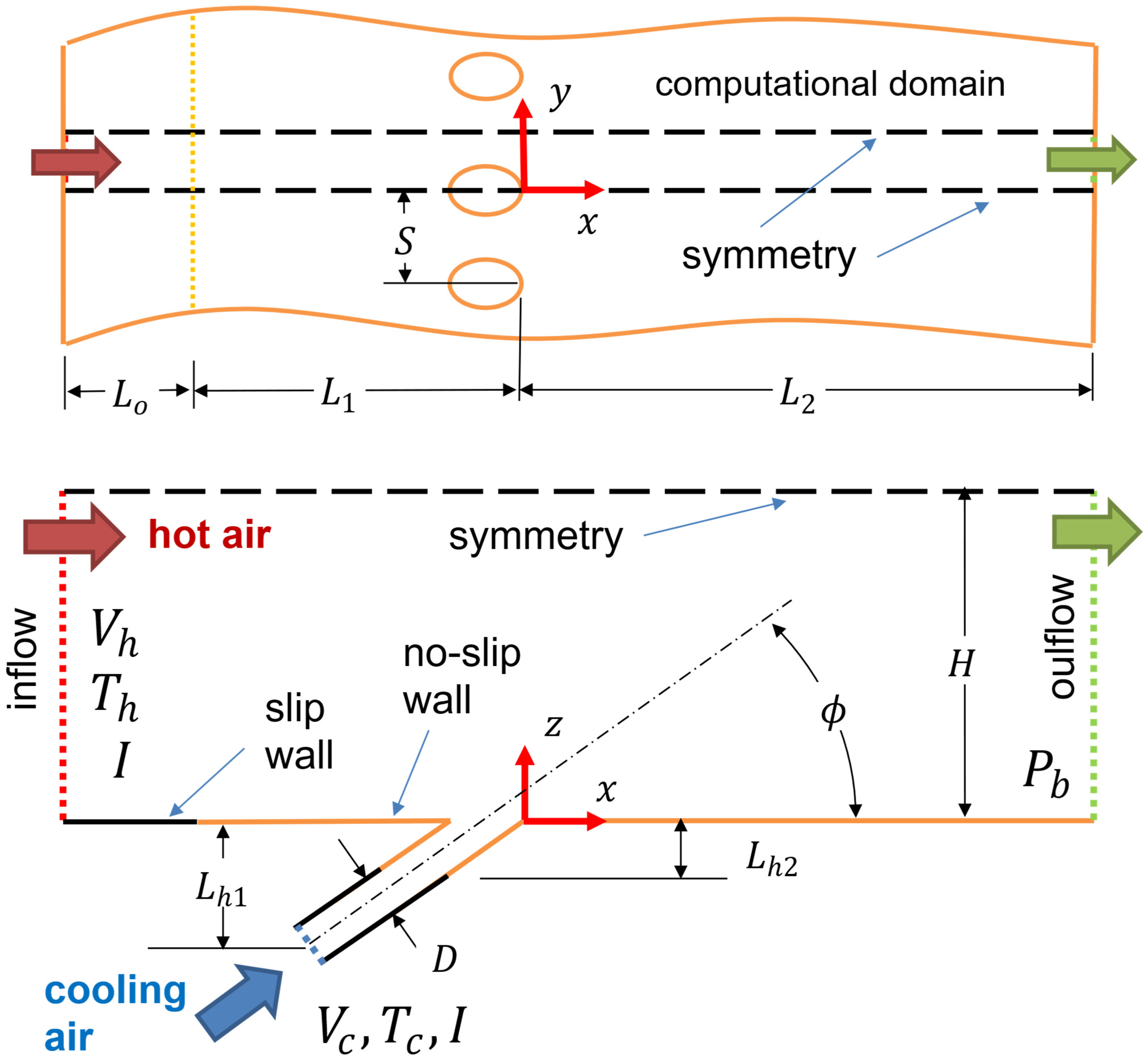
The film-cooled flat plate studied is shown in Figure 2. All dimensions are given in terms of D, the diameter of the film-cooling hole (D = 1 mm). The plate being cooled has a length of L 1 + L 2 , where L 1 = 19.1 D and L 2 = 30 D . The one row of film-cooling holes in the plate is located at x = 0 , which is L 1 downstream of the plate’s leading edge. All holes are oriented at ϕ = 35 degrees with respect to the plate, spaced S = 3 D apart, with a length of L h 1 = L 3 / s i n ( ϕ ) = 6 D .
The plate with the one row of film-cooling holes is exposed to hot air that flows over it and is cooled by cooling air issuing through the holes to insulate the plate from the hot air. The hot air that approaches the plate has a uniform temperature of T h = 1800   K and a uniform velocity of V h = 24.5   m / s in the x-direction at x = ( L 0 + L 1 ) . At the inlet of the film-cooling hole, the cooling air enters with uniform temperature of T c = 1125   K and uniform velocity of V c = 7.65   m / s along the hole’s axis. Both the hot and cooling air have a uniform turbulence intensity of I = 0.2 % and a ratio of turbulent-to-laminar viscosity of μ t / μ = 10 at locations where they enter the flow domain (see Figure 2). The static pressure at x = L 2 is P b = 25 atms. These conditions give rise to density, velocity, blowing, and momentum ratios of 1.6, 0.31, 0.50, and 0.16, respectively.
All surfaces on the plate and in the film-cooling hole are no-slip except for a section of the film-cooling hole below z = L 4 with L 4 = 2 D , where free-slip was imposed. The surface between x = ( L 0 + L 1 ) and x = L 1 at y = 0 , where the hot air approaches the leading edge of the plate was also modeled as free-slip. The thermal condition imposed on all free-slip surfaces was adiabatic. The thermal condition imposed on the no-slip walls was either adiabatic ( q s = 0 ) or isothermal ( T s ) . Nine different values of T s between 1112   K and 1814   K were examined. Note that T s = 1112   K is less than T c so that q s < 0 everwhere on the plate’s surface, and that T s = 1814   K is greater than T h so that q s > 0 everywhere on the plate’s surface. For T s between T c and T h , there are regions on the film-cooled surface where q s < 0 , q s > 0 , and q s = 0 . The nine T s examined, summarized in Table 1, are organized into five groups. The reason for the grouping is explained in the Results Section.
The problem just described and shown in Figure 2 is symmetric about planes at y = 0 , y = S / 2 , and z = H with H = 27 D , where H is much greater than the boundary-layer thickness and penetration of the film-cooling jet into the hot air. The computational domain employed in the CFD analysis is the one bounded by these symmetry planes, the inflow and outflow boundaries at x = ( L o + L 1 ) and x = L 2 , the inlet of the cooling hole, and all solid surfaces.

3. Problem Formulation and Numerical Method of Solution

The film-cooling problem described in the previous section was modeled by Reynolds-averaged Navier–Stokes (RANS)—namely, the time-averaged continuity, Navier–Stokes, and energy equations—where only steady-state solutions were sought [45]. Though the flow is compressible because of the huge temperature differences among T c , T h , and T s , both the compressible and the incompressible versions of the RANS equations were utilized to understand the effects of fluid properties on the flow and heat transfer, as well as the coupling and decoupling among the RANS equations. In both cases, the hot and cooling air were modeled as dry.
For the compressible formulation, the hot and cooling air were taken to be thermally perfect with temperature-dependent properties for dynamic viscosity, thermal conductivity, and constant-pressure specific-heat capacity. The temperature dependence of these properties was implemented as polynomials of degrees 3, 4, and 5, respectively, constructed from data of air between 200   K and 2000   K from [46].
For the incompressible formulation, the density ( ρ ) of the hot and cooling air was constant at ρ = P b / R T h , where R is the gas constant of air. All transport ( μ and k ) and thermodynamic ( C p ) properties were also constants, with μ and k evaluated at T h , and C p computed from the Prandtl number ( P r = μ C p / k ). On the Prandtl number, both the laminar and turbulent Prandtl numbers were set to unity (i.e., P r = P r t = 1 ) so that the thermal and the momentum diffusivities are the same. Since all transport properties were constants, the continuity and Navier–Stokes equations were decoupled from the energy equation in the solution procedure. Once velocity and the pressure gradients were obtained from the continuity and momentum equations, they were used to obtain temperature from the thermal energy equation.
For both the incompressible and compressible formulations, the effects of turbulence were modeled by the two-equation realizable k ε model [47] in the fully turbulent region and by the one-equation model of Chen & Patel [48,49] in the near-wall region (i.e., wall functions were not used). Again, it is noted that though turbulence modeling in RANS is a challenge, the questions this study seeks to address apply to both laminar and turbulent flows. Thus, turbulence is not the source of the challenge in obtaining T r e f and h . To ensure consistency when comparing methods for obtaining T r e f and h , the same turbulence model was used throughout this study.
Solutions to the Reynolds-averaged equations and the turbulence models were obtained by using Version 2021 R2 of Ansys® Fluent [50]. All inviscid terms were approximated by second-order upwind differences, and all diffusion terms by second-order central differences. Though only steady-state solutions were of interest, the segregated method was not used. The fully coupled pressure-based algorithm with Rhie–Chow distance-based flux interpolation [51] was used instead because it converged faster. The coupled algorithm enabled faster convergence because with a cooling-air to hot-air density ratio of 1.6, the flow is highly compressible so that the continuity and momentum equations are strongly coupled to the energy equation. In all cases, computations were continued until the residuals plateaued to ensure convergence to the steady state had been reached. At convergence, the normalized residuals were less than 10 5 for the discretized continuity and ε equations and less than 10 10 for all other discretized governing equations.

4. Grid Sensitivity Study

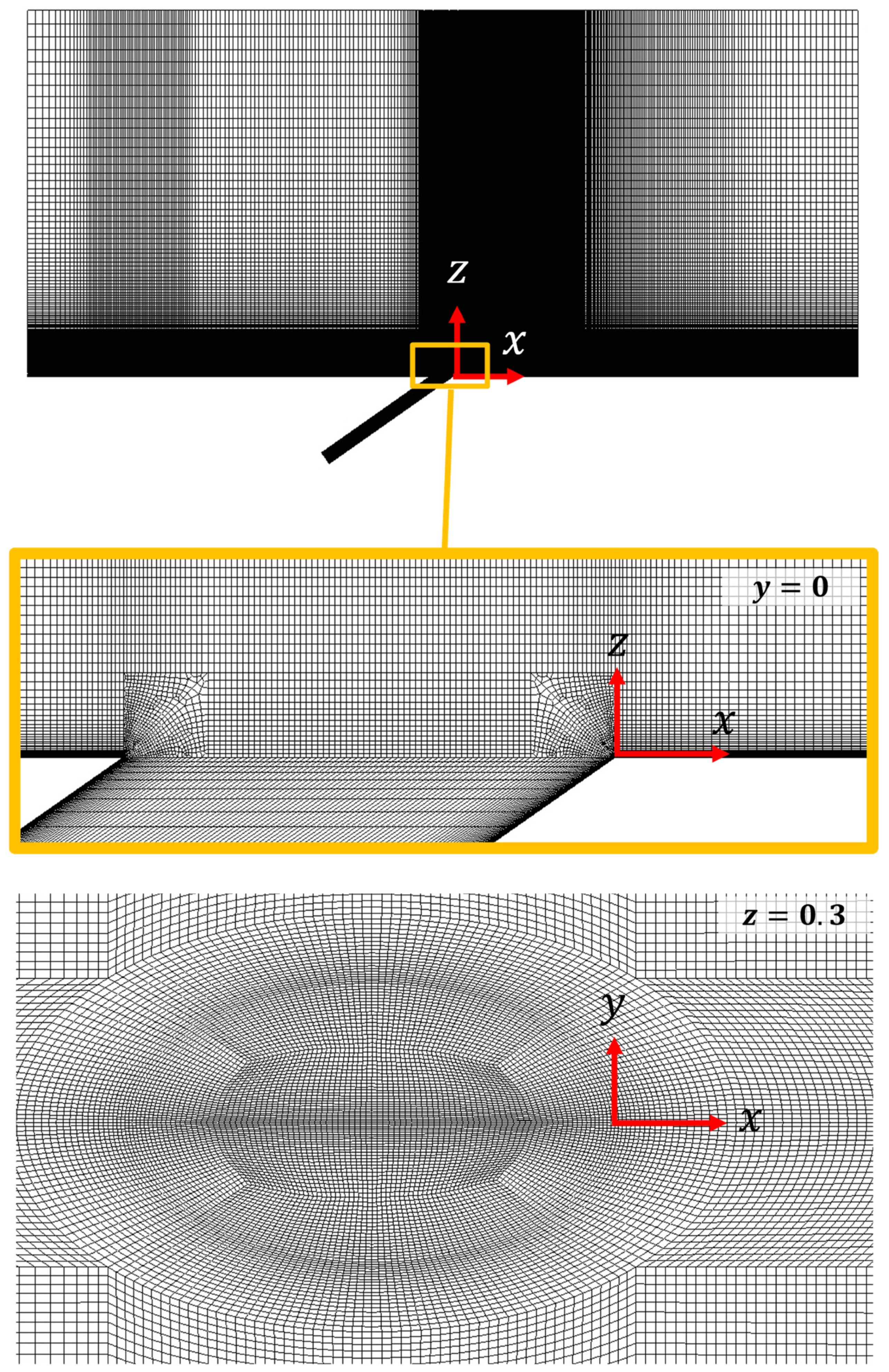
The baseline grid employed in this study is shown in Figure 3. It is mostly structured except for a small region that is unstructured. The unstructured grid smoothly connects the structured wrap-around grid about all solid surfaces, the structured grid in the film-cooling hole (H-H in the middle and O-H about the hole), and the structured grid above the plate (H-H). This grid system was selected to ensure all grid lines intersect the plate’s surface orthogonally so that q s = 0 can be accurately imposed if the wall is adiabatic, and q s can be accurately computed if the wall is isothermal. Grid points were clustered to resolve the boundary-layer flow above the plate, the flow in the film-cooling hole, the boundary-layer/cooling-jet interactions, and the locations on the film-cooled surface where T s T r e f = 0 and where q s = 0 .
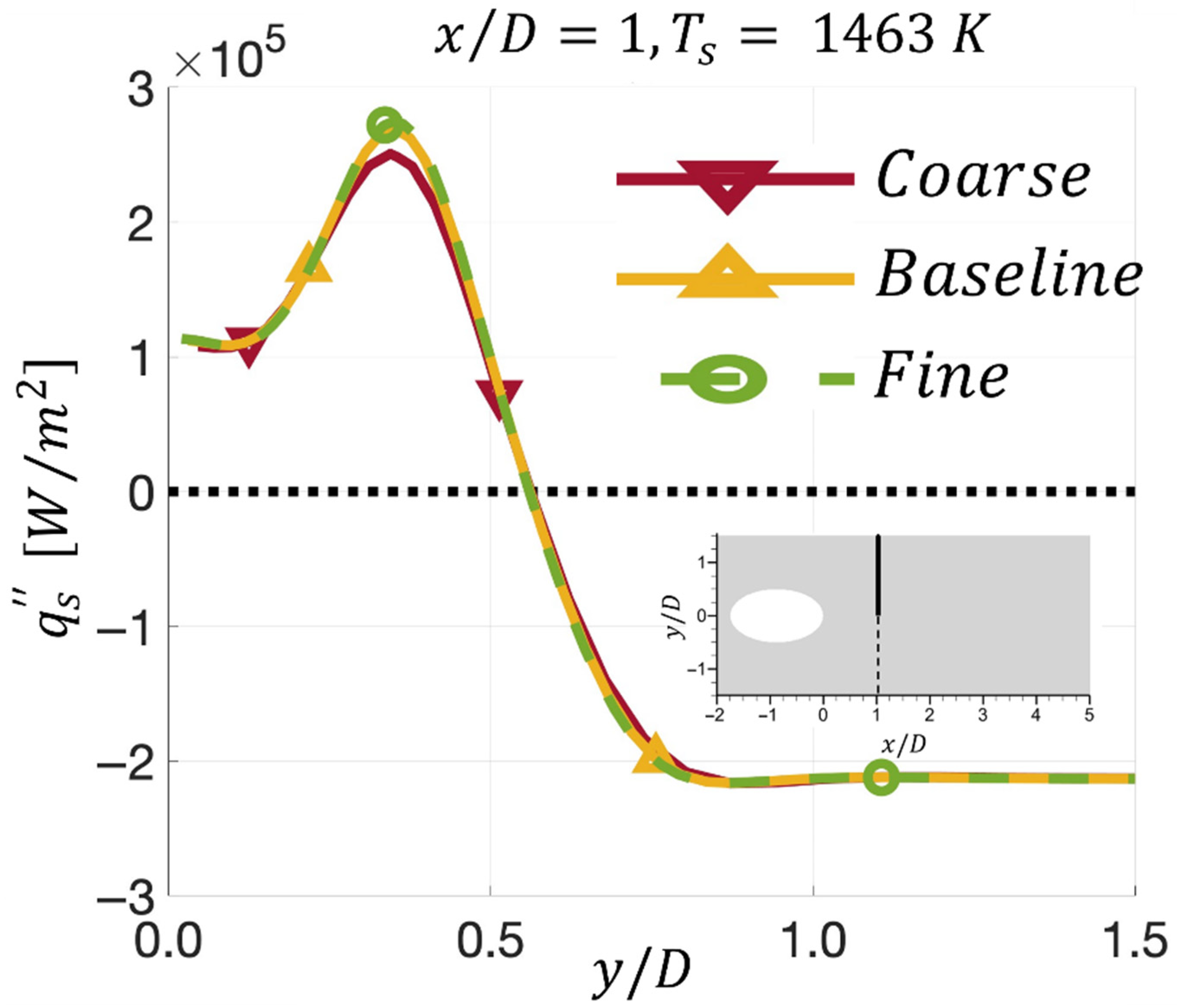
To ensure that the number of grid points used is sufficient to resolve the relevant features of the flow, a grid-sensitivity study was performed for a case with adiabatic walls to examine T A W and a case with isothermal walls ( T s = 1463   K , which gives rise to a temperature ratio of θ s = ( T h T s ) / ( T h T c ) = 0.5 ) to examine q s . The three grids used were as follows (Table 2): “coarse” with 1.72 million cells, “baseline” with 5.70 million cells, and “fine” with 20.3 million cells. For all three grids, y+ is less than unity for all cells next to solid surfaces. Also, the first three cells next to all solid surfaces have the same grid spacing normal to the surface.
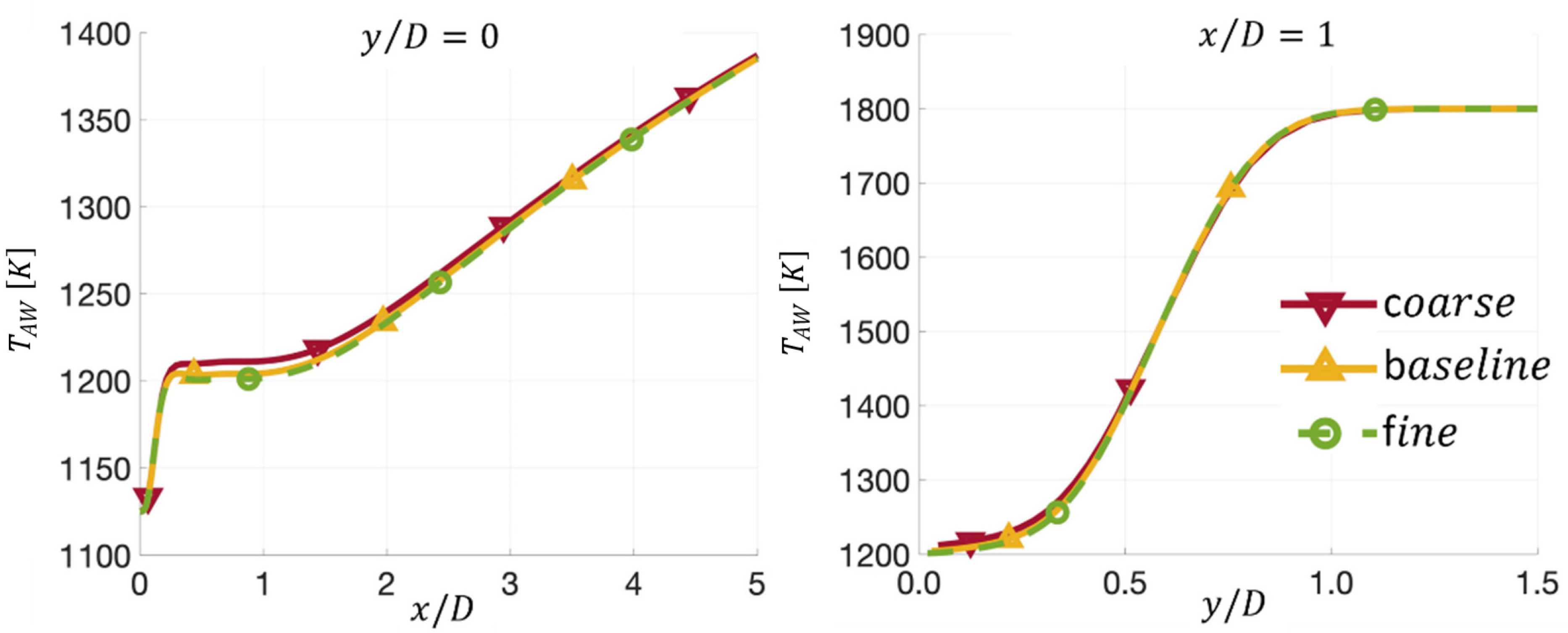
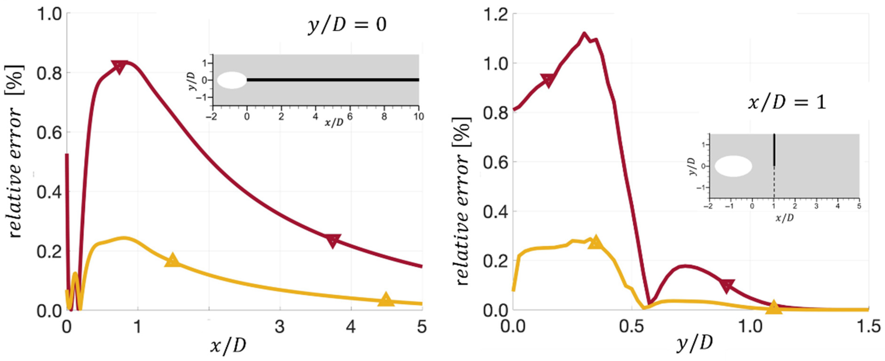
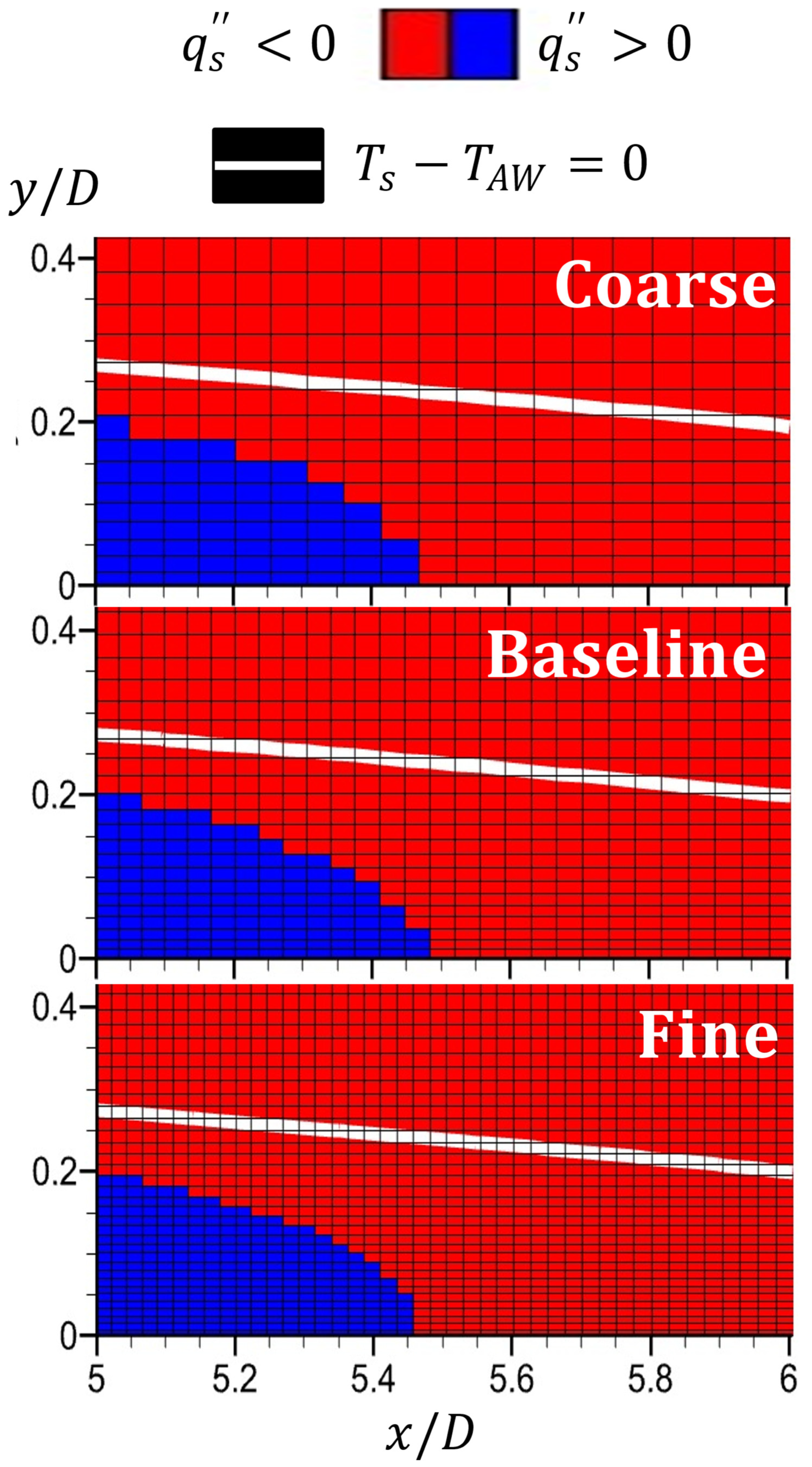
The results of the grid-sensitivity study are shown in Figure 4, Figure 5 and Figure 6. Figure 4 shows T A W obtained by using the coarse, baseline, and fine grids along x / D at y / D = 0 and y / D at x / D = 1 . From this figure, it can be seen that T A W obtained on the baseline grid is nearly the same as that obtained on the fine grid. The maximum relative difference is less than 0.3%. Figure 5 shows q s obtained on the three grids along y / D at x / D = 1 . From this figure, the solutions obtained on the baseline and fine grids are nearly identical. The largest absolute differences occur at y / D = 0.0 and y / D = 0.4 , and the corresponding relative differences are less than 0.2%. Figure 6 shows the locations on the film-cooled surface where T s T A W = 0 (white line) and where q s = 0 (the interface where RED and BLUE meet). From this figure, the baseline grid can be seen to be adequate in resolving those locations. Based on the aforementioned information, the baseline grid was used to generate all solutions presented in the Results Section.

5. Results

The results obtained to address the objectives of this study are presented in this section. First, T r e f and h obtained by the AW and LE methods are examined and assessed according to the requirements outlined by Peck et al. [43], namely Requirements A ( q s = 0 where T r e f T s = 0 ), B (continuity of h across T s T r e f = 0 ), and C (uniqueness). Next, the foundation of the SS method for obtaining T r e f and h is examined. This method is then used to assess the accuracy of T r e f and h obtained by using the AW and LE methods. In the subsections that follow, all results presented were obtained by using the compressible formulation—unless mentioned otherwise.

5.1. T r e f   a n d   h Obtained by the Adiabatic-Wall (AW) Method

To examine the AW method, one simulation was performed with an adiabatic-wall boundary condition (BC) imposed on all solid surfaces to obtain T A W , and four simulations were performed with isothermal-wall BC to obtain h A W = q s / ( T s T A W ) . The wall temperatures used for the isothermal-wall simulations are given by Set 1 in Table 1.
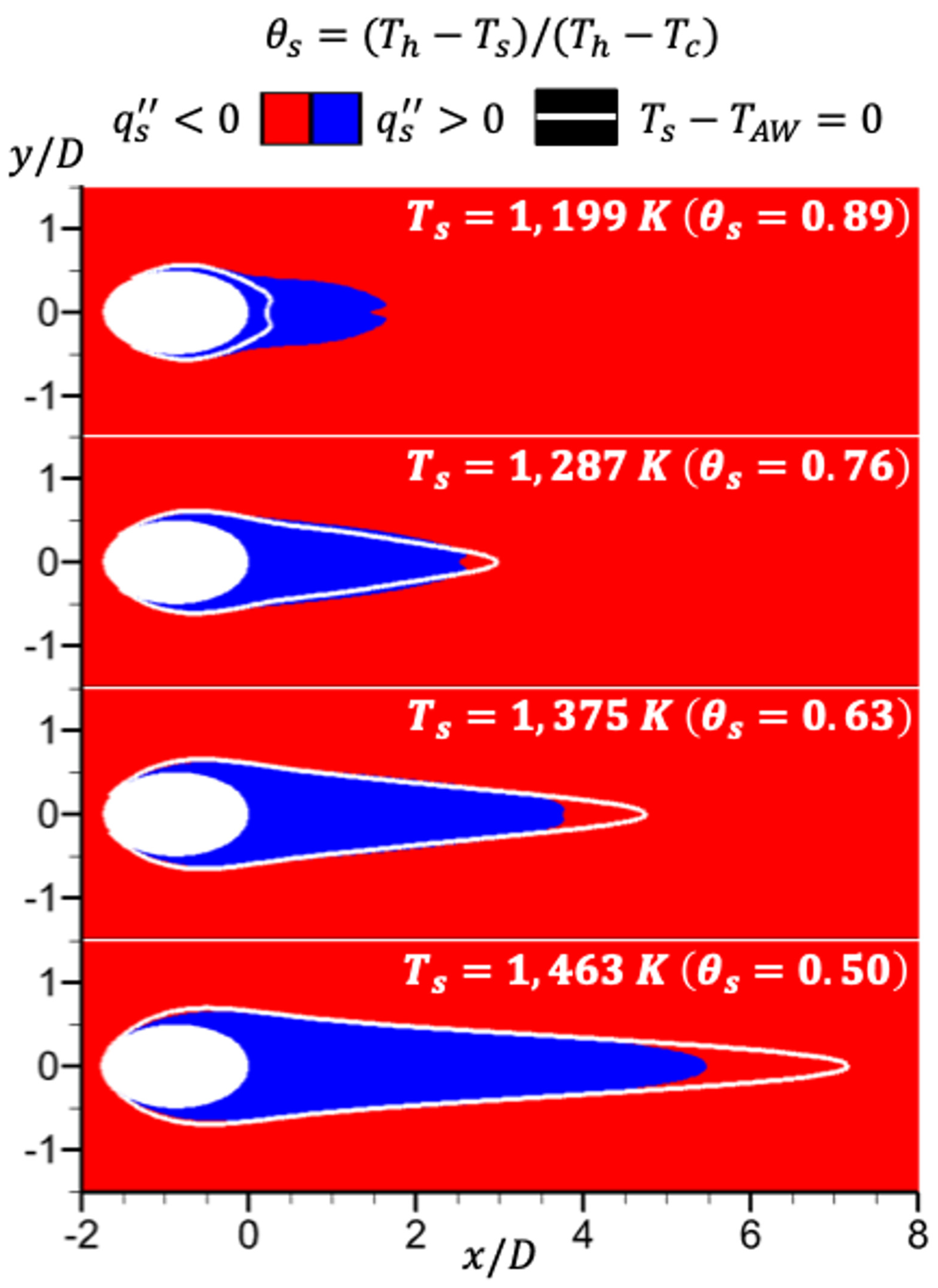
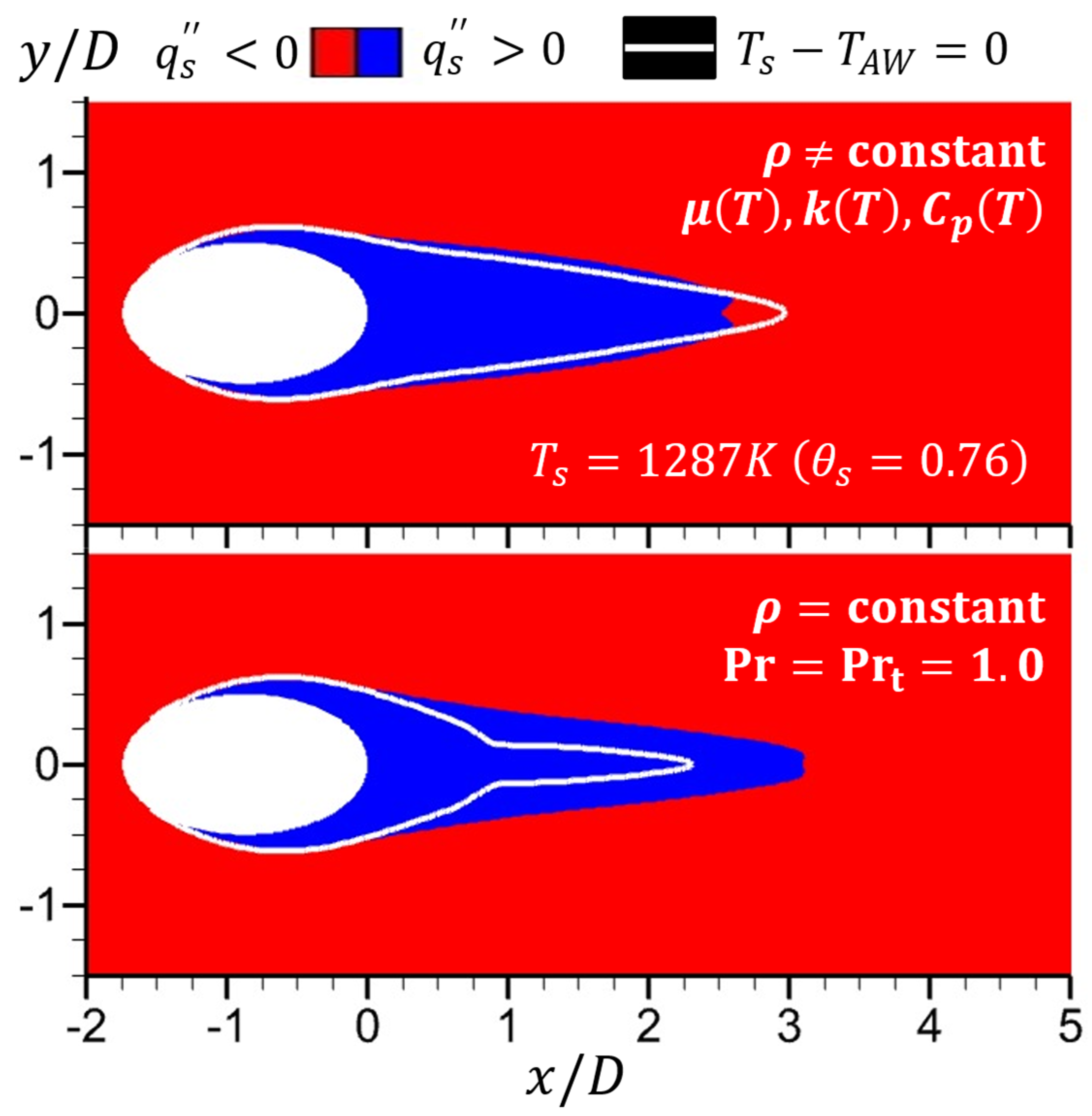
Since there is only one temperature distribution on an adiabatic wall for a given flow condition, T r e f = T A W is unique and satisfies Requirement C. To assess Requirement A, the locations where q s = 0 and where T s T A W = 0 need to be determined, and they are shown in Figure 7. In this figure, the white lines are where T s T A W = 0 , and the interface that separates the blue and red regions is where q s = 0 . From this figure, it can be seen that the line where T s T A W = 0 and the line where q s = 0 do not coincide for any of the T s values evaluated. Thus, T A W does not meet Requirement A. Also, h A W = q s / T s T A W approaches ± , where T s T A W = 0 , but q s 0 . Thus, the AW method also does not meet Requirement B.
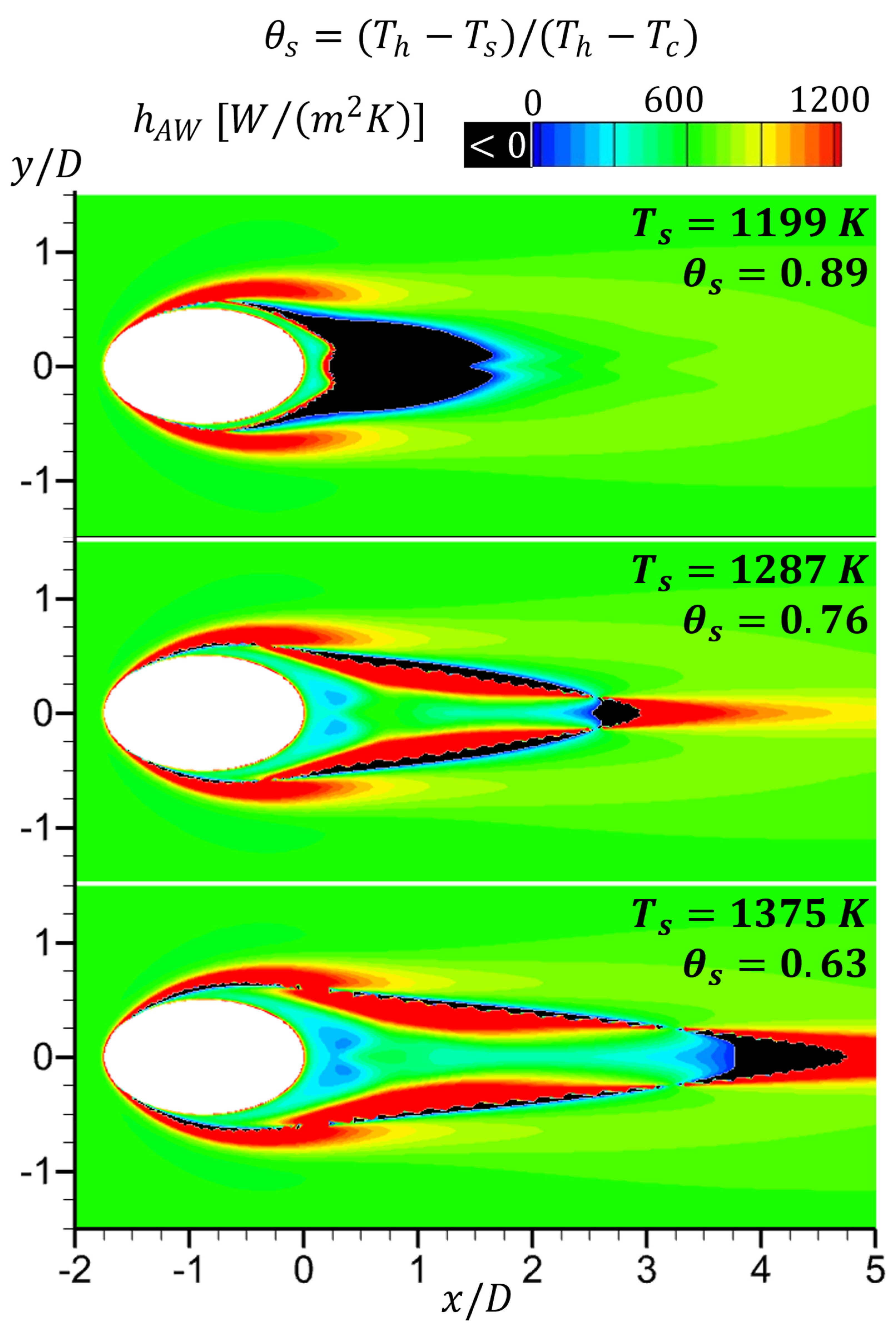
Figure 8 shows h A W obtained with three different wall surface temperatures: T s = 1199   K , 1287   K , and 1375   K . From this figure, h A W can be seen to depend on the value of T s . Also, since q s 0 where T s T A W = 0 ,   h A W can be negative on a significant portion of the surface (see region marked in black). A negative h A W implies that heat is flowing from a colder temperature to a hotter temperature, which is not physical as it violates the second law of thermodynamics. Thus, not only does T A W violate Requirements A and B, it could produce values of h that are nonphysical if q s can switch signs on the non-adiabatic surface.
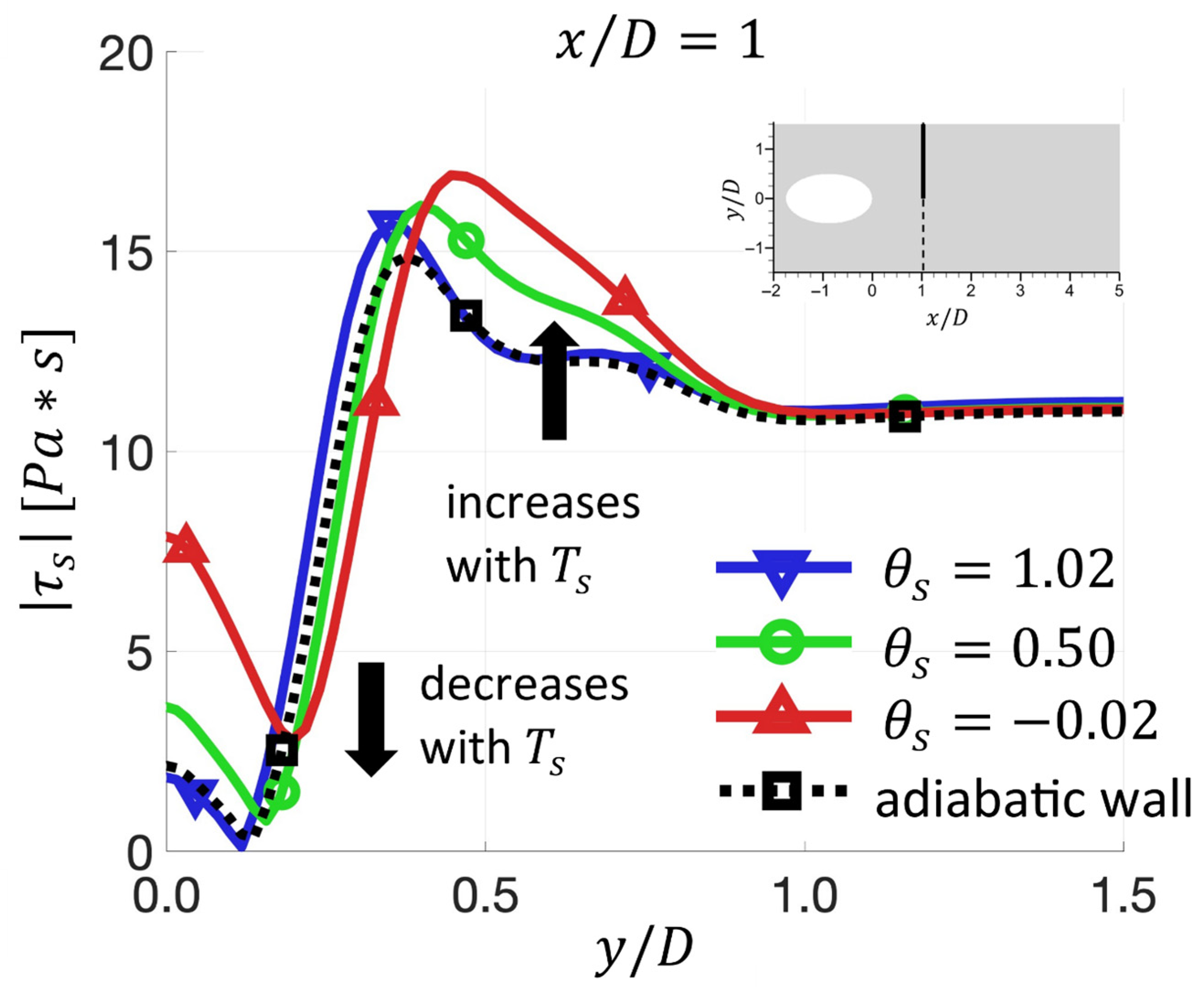
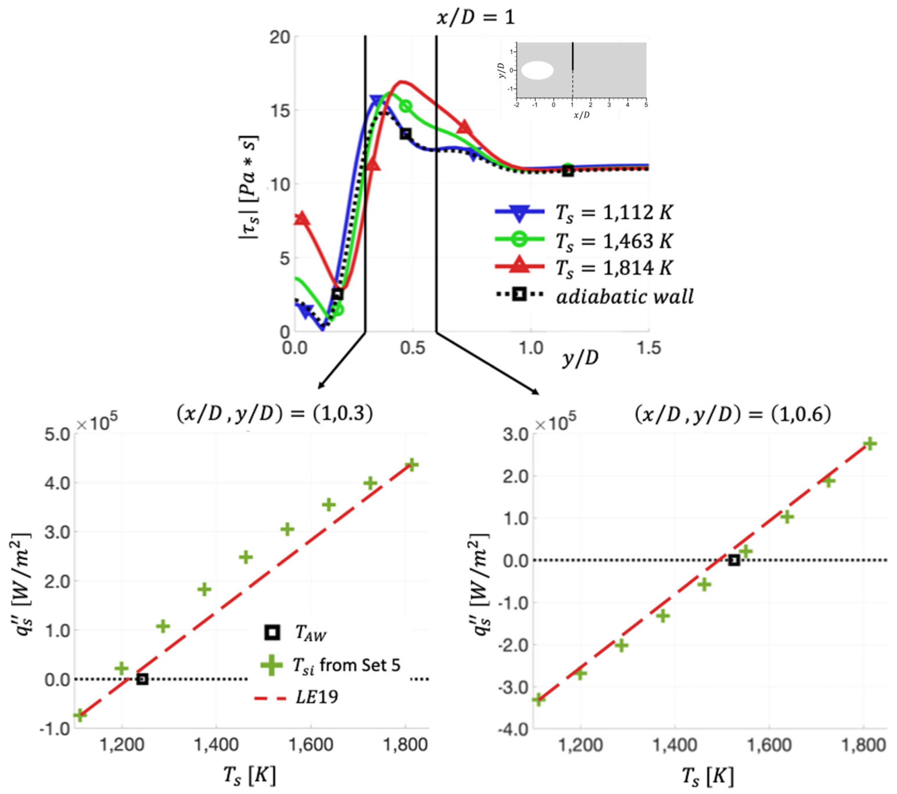
The AW method provides incorrect T r e f and h because an adiabatic wall and a non-adiabatic wall (such as an isothermal wall) produce different temperature distributions about the surface exposed to hot-air and cooling-air flows—even though the density and blowing ratios along with T h , T c , and the geometry are identical. Figure 9 shows the magnitude of the shear stress τ s on an adiabatic wall and on an isothermal wall with three different temperatures ( T s = 1112   K < T c ,   T s = 1463   K , and T s = 1814   K > T h ) along y / D at x / D = 1 . From this figure, the distribution of τ s can be seen to be a strong function of T s or q s , especially in the region where the cooling air and the hot air interact. Thus, T s or q s strongly affects the nature of the flow and hence the heat transfer, and T A W obtained on an adiabatic wall could not capture these physics.
Though the locations where q s = 0 and T s T A W = 0 do not match, they are not too far apart from each other, as shown in Figure 7. Thus, it is of interest to see if they will match if (1) the flow is incompressible with constant viscosity so the thermal-energy equation can be decoupled from the continuity and the Navier–Stokes equations and (2) the laminar and turbulent Prandtl numbers are equal to unity so that the thermal and momentum diffusivities are the same. Though these are clearly incorrect assumptions for this flow, they were invoked to examine the effects of density and diffusivities on where q s = 0 and where T s T A W = 0 . Thus, two simulations were performed with these assumptions, one with the adiabatic wall to obtain T A W and another with the isothermal wall at T s = 1467   K   θ s = 0.5 to obtain h A W . The results obtained, given in Figure 10, show where q s = 0 and where T s T A W = 0 still do not coincide—even though the flow fields for the adiabatic and isothermal walls are now identical. This shows that it is upstream surface heat transfer that determines the location where q s = 0 . This also shows that upstream surface heat transfer must be accounted for by any method used to determine T r e f .
With the role of heat transfer on T r e f recognized, the trend where q s = 0 and where T s T A W = 0 , as shown in Figure 7, can be explained. As T s on the surface is increased, more heat transfer is needed to heat the cooling air from T c to T s so where q s = 0 and where T s T A W shift further and further downstream of the film-cooling hole along x / D at y / D = 0 . The mismatch between where q s = 0 and T s T A W = 0 along x / D at y / D = 0 also increases with T s because with the isothermal wall, where T s > T c , the cooling air is heated by both the hot air and the wall, whereas with the adiabatic wall, the cooling air is only heated by the hot air. The exception is the case with T s = 1199   K , where q s = 0 is located downstream of where T s T A W = 0 . This is because with T s only slightly higher than T c but much lower than T h , hot air above the isothermal wall is cooled by the wall, so heat transfer to the cooling air from the wall and from the hot air is lower than the heat transfer to the cooling air from the hot air when the wall is adiabatic. To summarize, locations where q s = 0 on an isothermal wall depend on upstream heat transfer from the wall and from the hot air, whereas the locations where T s T A W = 0 do not account for the heat transfer from the wall.

5.2. T r e f   a n d   h Obtained by the Linear-Extrapolation (LE) Method

The LE method given by Equations (2)–(4) is again assessed by using the three requirements from Ref. [43]. Though only one pair of ( T s ,   q s ) is needed to determine T r e f , L E and h L E , five q s were generated by using the five T s values from Set 2 in Table 1 (i.e., T s 1 , T s 3 , T s 5 , T s 7 , T s 9 ). From ( T s i ,   q s i ) with i = 1 ,   3 ,   5 ,   7 , and 9 , three pairs of ( T s i ,   q s i ) were constructed—denoted as L E i j = L E 15 ,   L E 37 , and L E 59 —to obtain T r e f , L E i j and h L E i j .
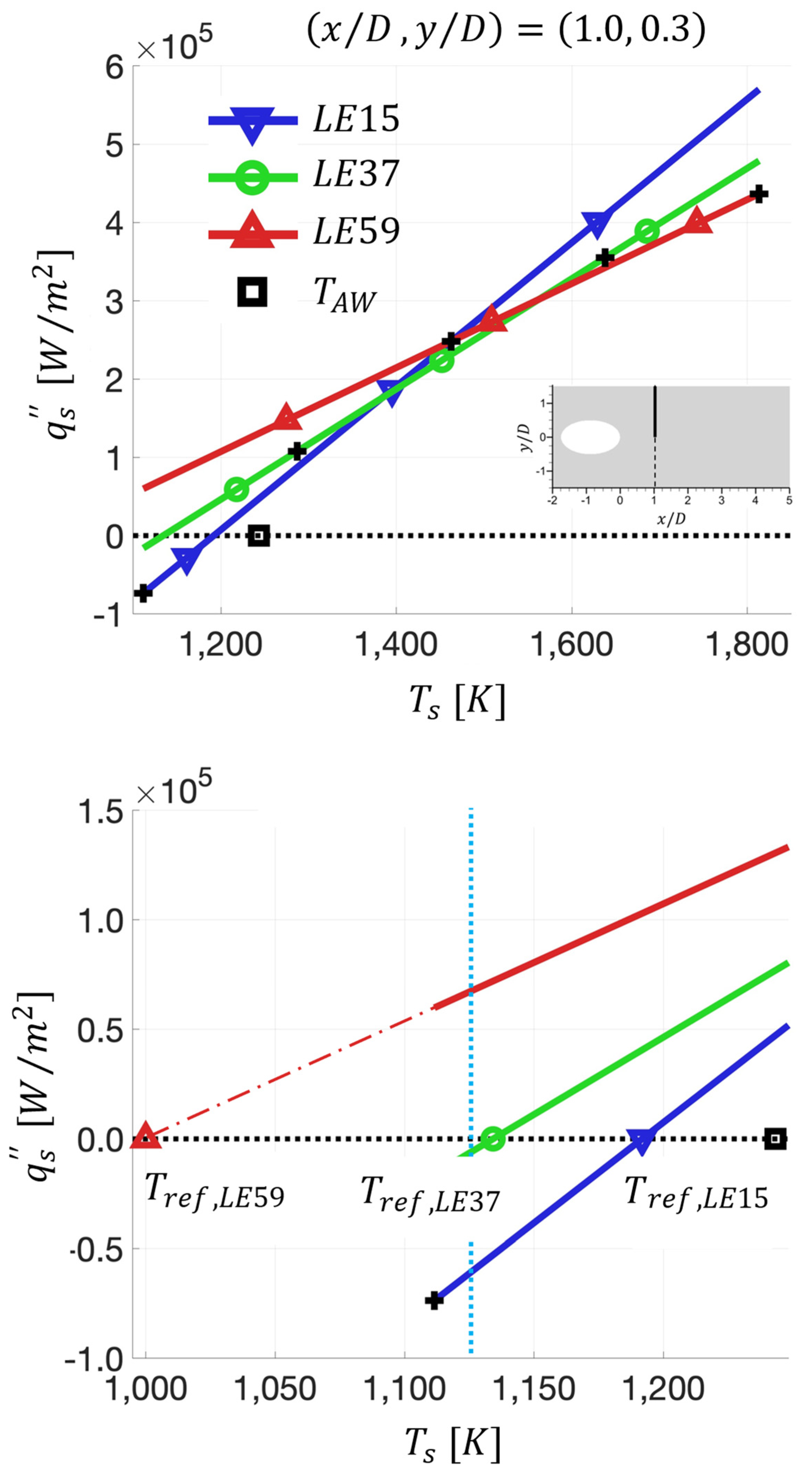
Figure 11 shows q s as a function of T s at x / D , y / D = 1.0 ,   0.3 , obtained by using L E 15 ,   L E 37 , and L E 59 , which can be seen to be three straight lines—each with a different slope, h L E i j = ( q s i q s j ) / ( T s i T s j ) and intercept T r e f , L E i j = ( q s i T s j q s j T s i ) / ( T s i T s j ) . By not obtaining a unique line, the LE method does not satisfy Requirement C. However, since Equation (2) obtains T r e f , L E by finding the temperature that makes q s = 0 , locations where T s T r e f , L E = 0 and q s = 0 do coincide. Thus, Requirement A is satisfied. Also, since the slope of the straight line constructed by a pair of ( T s i ,   q s i ) is h L E , and it is continuous across q s = 0 as shown in Figure 11, Requirement B is satisfied. Though T r e f , L E and h L E obtained by the LE method satisfy Requirements A and B, the T r e f , L E obtained can be nonphysical. This can be seen in Figure 11, where T r e f , L E 59 is less than T c = 1125   K , and this violates the second law of thermodynamics. Also, the locations where q s = 0 predicted by the LE method will not in general match the location where q s is truly zero for the nonadiabatic-wall problem studied.
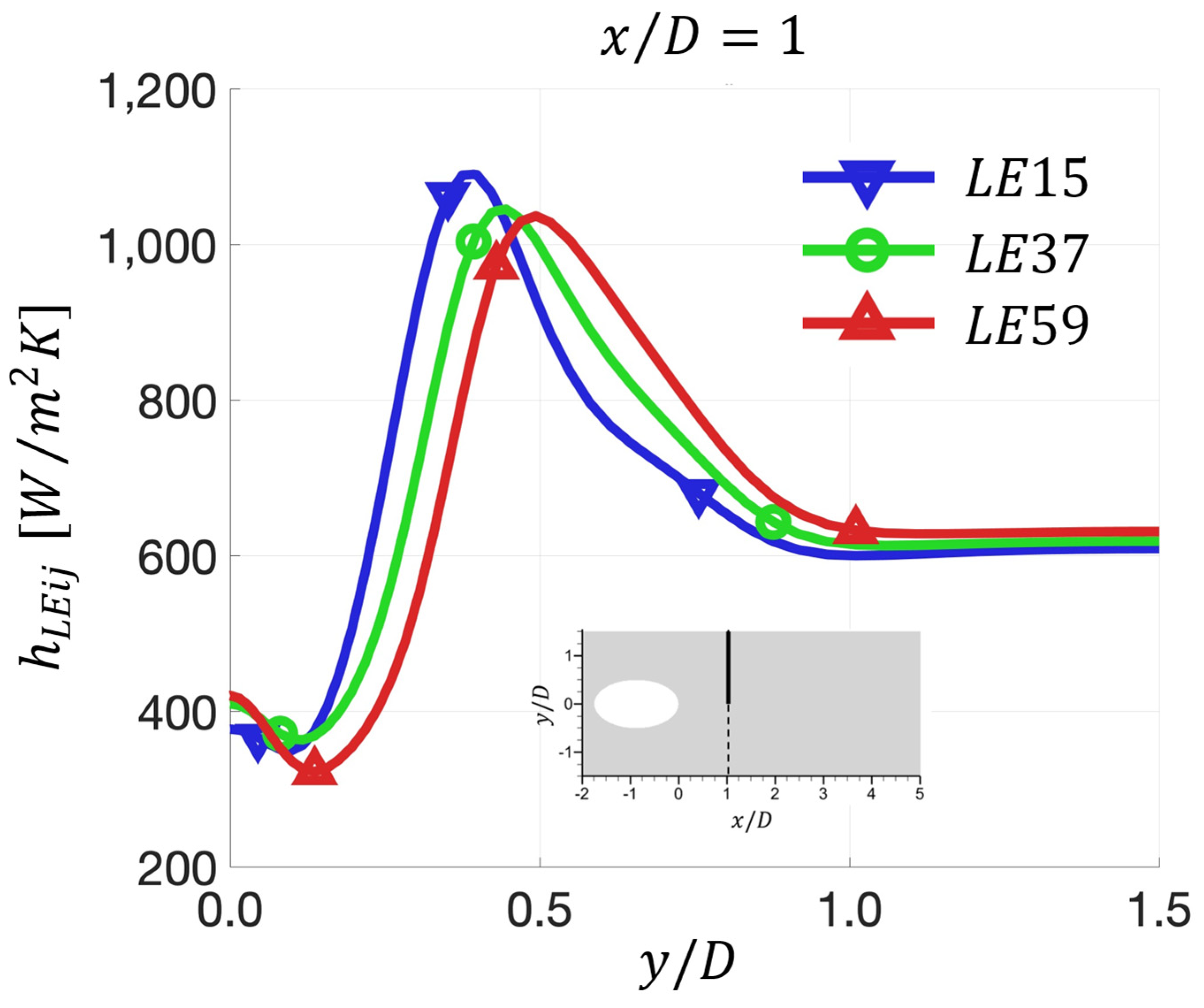
Figure 12 shows h L E i j obtained by the three pairs of T s , q s along y / D at x / D = 1 to be a function of T s . Thus, the assumption invoked by the LE method, given by Equation (2), is incorrect; namely, T r e f and h do not just depend on the ratio of ( q s , 2 T s 1 q s , 1 T s 2 ) or ( q s i q s j ) to ( T s i T s j ), they also depend on T s .
Since linearity was invoked in Equation (2), this begs the question: Could the dependence of h L E i j on T s be captured by a nonlinear correction, such as a temperature ratio raised to a power of n as proposed in Refs. [1,18]?
T s / T r e f n
However, inspection of Figure 13 shows the slope, which equals h E L , to increase as T s increases at some locations and to decrease as T s increases at other locations—indicating the presence of maximums and minimums. This trend closely follows the magnitude of the wall shear stress shown in Figure 9 (also repeated in Figure 13) and is due to heat transfer on the film-cooled surface, changing the flow field near the surface. Thus, a function such as Equation (6), which has the same value of “ n ” for the entire surface, does not work. There may even be locations where h does not follow a power law relationship with T s / T r e f , such as Equation (6), suggested by Figure 12 at x / D = 1 and y / D 0.45 where h L E 37 is greater than both h L E 15 and h L E 59 .

5.3. T r e f   a n d   h Obtained by the State-Space (SS) Method

Before presenting results obtained by the method developed by Peck et al. [43], this study seeks to establish the foundation of their method, which was not presented in Ref. [43]. To do so, consider the film-cooling problem depicted in Figure 2 with the isothermal wall at any temperature T s . For a given flow condition with hot-air flow at T h and cooling-air flow at T c , there is a unique distribution of heat flux q s ( x , y ) that corresponds to T s . Since q s ( x , y ) and T s are related by Newton’s law of cooling, there is a correspondingly unique distribution of either h ( x , y ) or T r e f ( x ,   y ) for this problem (i.e., once h is known, T r e f is known and vice versa). In this study, T r e f ( x ,   y ) is sought, and h is obtained from Equation (1) once T r e f ( x ,   y ) is obtained.
To examine the effect of T s on T r e f ( x , y ) , consider how q s ( x , y ) changes when T s is changed by the following equation:
d q s = d q s d T s d T s
Since q s and T s are related by Newton’s law of cooling given by Equation (1), Equation (7) becomes
d q s = d q s d T s d T s = d h T s T r e f d q s = d q s d T s d T s = T s T r e f ( x , y ) d h d T s + h ( 1 d T r e f d T s ) d T s
Thus,
d q s d T s = T s T r e f ( x , y ) d h d T s + h ( 1 d T r e f d T s ) = F ( T s , x ,   y )
Without loss of generality, suppose
T s = T s ψ = a ψ + b
where a and b are constants with unit K; ψ is dimensionless; and each value of ψ represents a different isothermal wall T s from T c to T h . Integrating Equation (7) with Equations (8) and (9) yields
q s x , y , ψ = T r e f x , y T s F T s ( ψ ) ,   x , y d T s     = ψ T r e f ψ F ( ψ , x ,   y ) d T s d ψ   d ψ = ψ T r e f ψ a F ( ψ , x ,   y )   d ψ
where
q s x , y , ψ T r e f = 0
The ψ that makes q s equal to zero at ( x , y ) , denoted as ψ T r e f , yields the reference temperature; i.e., T r e f = T s ( ψ T r e f ) at x , y . Thus, T r e f ( x ,   y ) obtained by Equation (10) and h ( x , y ) obtained by Equation (1) satisfy Requirements A and B. Since T s ( ψ ) given by Equation (9) is a monotonic function, and the flow and heat transfer on the film-cooled plate is single-valued and continuous, F ( ψ , x ,   y ) is single-valued and continuous so that the T r e f ( x , y ) and the h ( x , y ) obtained are unique, which satisfies Requirement C.
When Equation (10) is integrated over the entire surface of the film-cooled plate, the upstream heat transfer and how T s affect the flow and heat transfer are accounted for. In this study, the method of Peck et al. [43] is referred to as the state-space (SS) method. This is because the “integrated” Equation (10) examines the entire state space of isothermal surface temperatures T s ( ψ ) from T c to T h at all location x ,   y on the surface. The T r e f and h obtained by this method are denoted as T r e f , S S and h S S . Note that the subscript “ A W ” was not used to differentiate “reference temperature” from “adiabatic or recovery temperature”.
For the film-cooling problem studied, the state-space method obtains T r e f , S S and h S S —computationally or experimentally—in the following six steps:
1.
The first step is to discretize ψ in Equation (9) to produce N isothermal-wall temperature states, denoted as T s i = T s ( ψ i ) , where i = 1 ,   2 ,   , N . The T s i states chosen must include one temperature lower than the lowest temperature in the flow field (i.e., T c ) and one temperature higher than the highest temperature in the flow field (i.e., T h ) to ensure that the entire state space is accounted for. In this study, Equation (9) was discretized as follows:
T s i = T s ψ i = a ψ i + b
ψ i = i ,   i = 1 ,   2 ,   ,   N
where a = 87.80   K , b = 1023.75   K , and N = 9 . Note that T s 1 = T ψ 1 = 1024   K , which is lower than T c , and T s 9 = T ψ 9 = 1814   K , which is higher than T h . Equation (11) with i = 1 ,   2 ,   ,   9 includes all T s values given in Table 1.
2.
The second step is to compute or measure q s i at every point on the surface of the film-cooled plate with isothermal wall temperature T s i , denoted as q s i x , y . Repeat for i = 1 ,   2 ,   , N . If there are uncertainties in the measurements, then multiple measurements should be made for each T s i , and the averaged q s i and T s i should be used in subsequent steps.
3.
The third step is to perform a transfinite interpolation of [ T s i , q s i ( x , y ) ] at i = 1 , 2 , , N , generated in Step 2, to construct a function G T ψ , q s x , y = 0 . In this study, cubic spline interpolation was used with the third derivative at T ( ψ 1 ) and T ( ψ N ) set to the third derivative at adjacent points, corresponding to the “Not-a-Knot” end condition [52].
4.
The fourth step is to use a root-finding routine for the function, G T ψ , q s x , y = 0 , to find the ψ at every point on the surface that makes q s x , y = 0 . The ψ that makes q s = 0 at x , y is denoted as ψ T r e f .
5.
The fifth step is to assign the temperature obtained in Step 4, namely, T s ψ at ( x , y ) , as T r e f , S S ( x , y ) .
6.
The sixth step is to calculate h S S at every point on the film-cooled surface by using Equation (1). At all locations where T s T r e f , S S 0 , h S S ( x , y ) = q s ( x , y ) / [ T s T r e f , S S x , y ] . At locations where T s T r e f , S S = 0 and q s = 0 , apply L’Hospital’s Rule so that h S S = q s / T s .
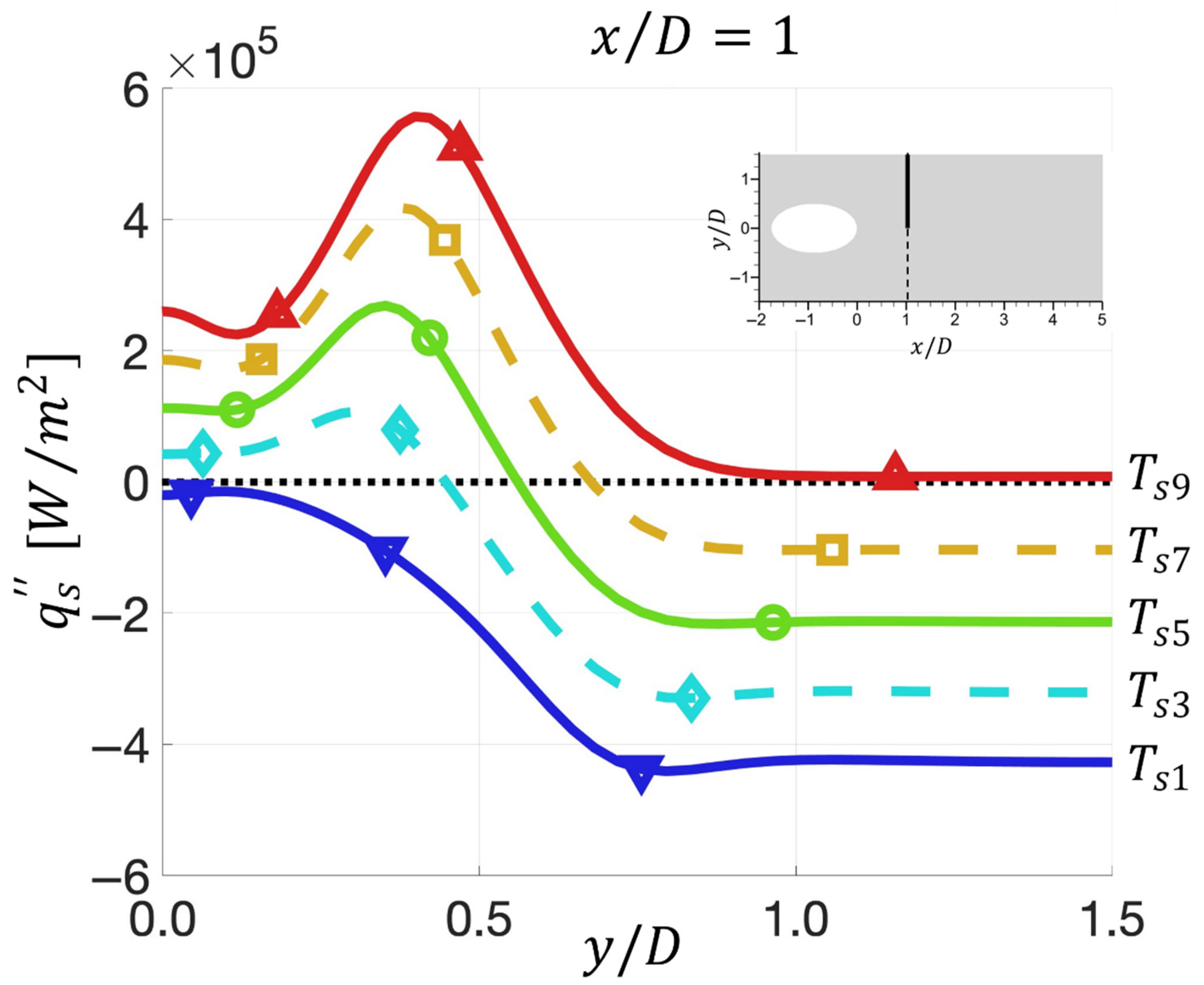
Figure 14 shows the interpolated q s x , y as a function of y / D at x / D = 1 for five T s i = T ( ψ i ) values given in Set 4 of Table 1. From this figure, the location y of T r e f , S S x = D , y = T s i could be found, and it is where T s i = T ( ψ i ) intersects with q s = 0 . With the function G T ψ ,   q s x , y = 0 constructed by transfinite interpolation in Step 3, T r e f , S S x , y can be found at every point on the surface. From Figure 14, it can be seen that T r e f , S S = T h at y / D > 1 , where the surface was not film cooled. At y / D < 1 , where the film-cooling flow and hot-air flow interact, T r e f increases from near T c at y / D = 0 to T h as y / D increases.
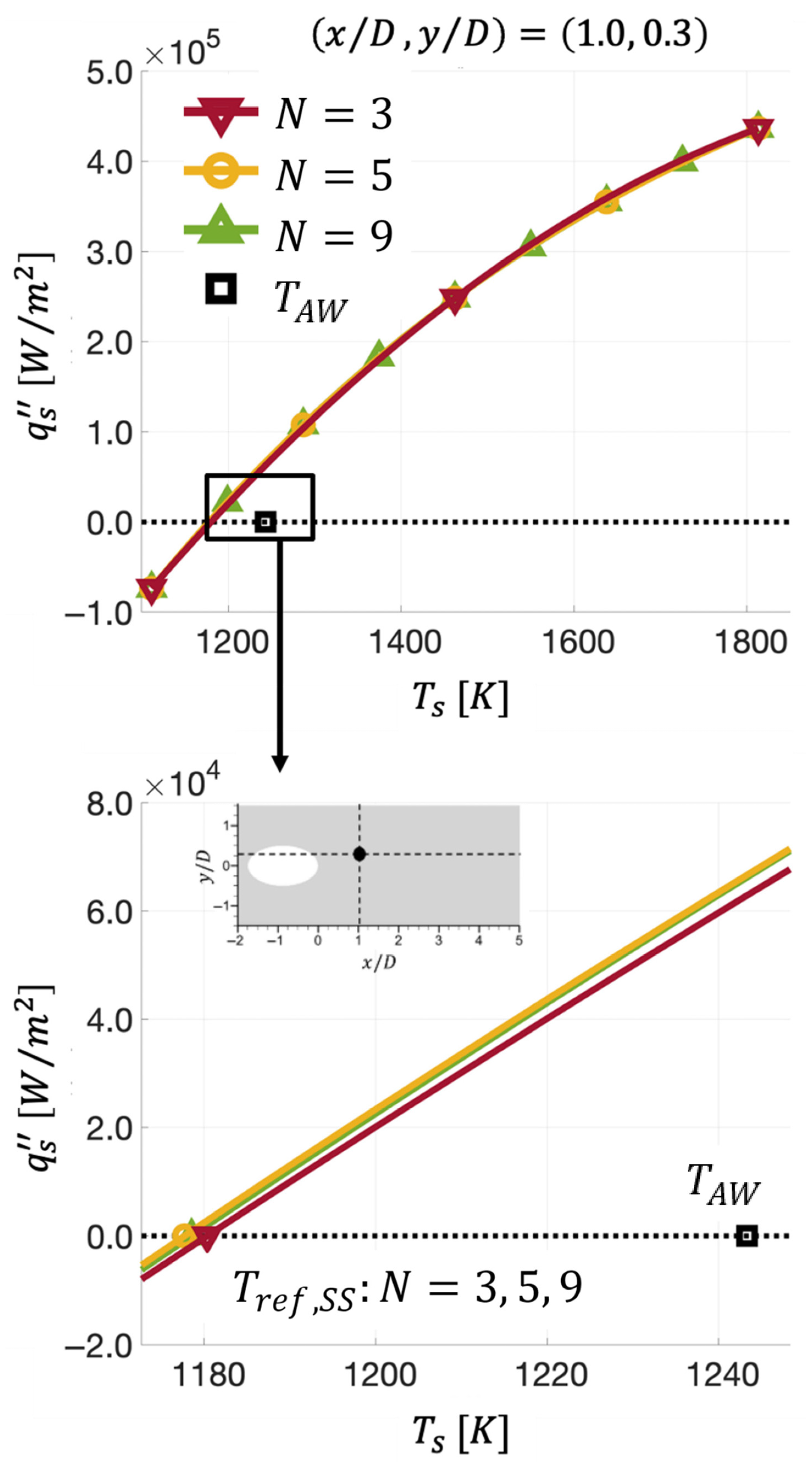
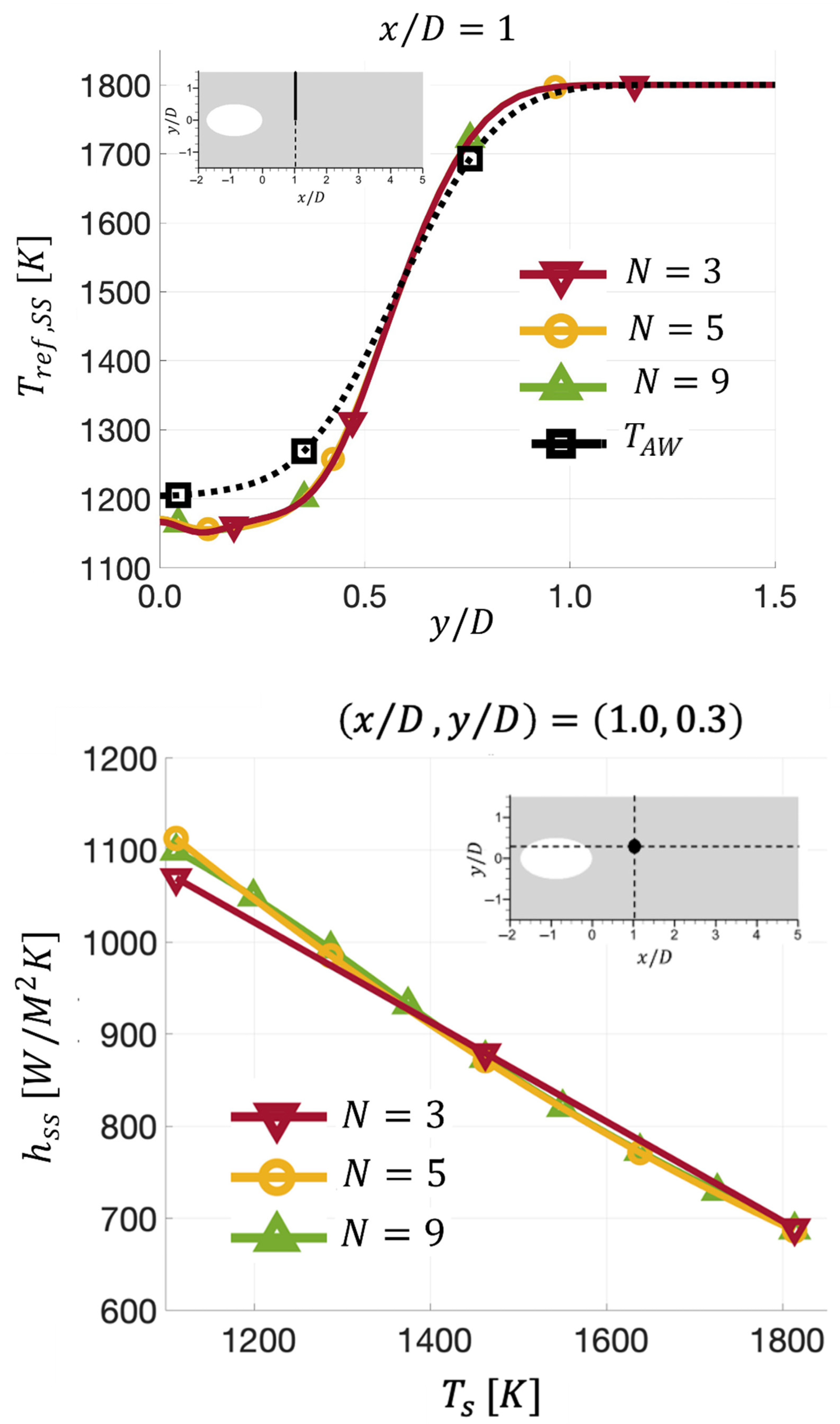
Peck et al. [43] showed that the accuracy and efficiency of the SS method depends on the size of N (i.e., the number of T s i states examined). To assess accuracy, this study examined N = 3 ,   5 , and 9 equally spaced states that correspond to Set 3 ( T s 1 ,   T s 5 ,   T s 9 ), Set 4 ( T s 1 ,   T s 3 , T s 5 ,   T S 7 ,   T s 9 ), and Set 5 ( T s 1 , T s 2 ,   T s 3 , T S 4 ,   T s 5 ,   T s 6 ,   T S 7 ,   T s 8 ,   T s 9 ) in Table 1, where T s i is given by Equation (9). Figure 15 shows q s ( x , y ) as a function of T s ( ψ ) and N at x , y = D ,   0.3 D from Step 3 of the SS method, and Figure 16 shows T r e f , S S ( x , y ) and h s s ( x , y ) as a function of y / D at x / D = 1 and N from Steps 4 and 5 of the SS method. From these two figures, q s ( x , y ) , T r e f , S S ( x , y ) , and h S S ( x , y ) obtained with N = 5 and 9 are nearly identical. With N = 3 , the maximum error in T r e f , S S ( x , y ) relative to N = 9 is less than 1%. Thus, N = 3 should be adequate in obtaining T r e f , S S ( x , y ) , albeit N = 5 as suggested by Peck et al. [43] would yield an even more accurate h S S ( x , y ) , that meets requirements A, B, and C.
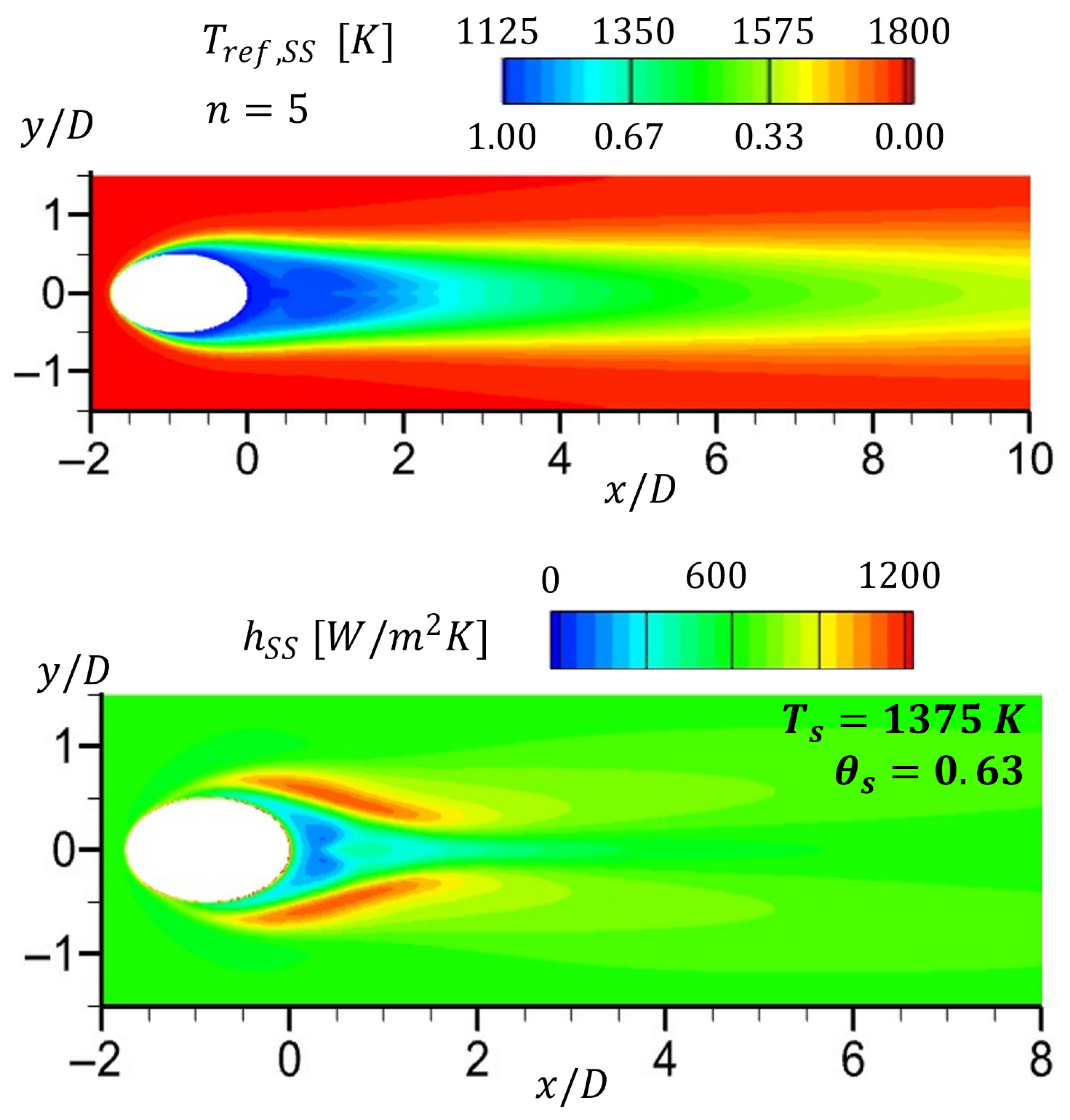
Figure 17 shows T r e f , S S ( x , y ) obtained on the film-cooled surface with a transfinite interpolation base on N = 5 and the h s s ( x , y ) obtained with T s = 1375 K by using Equation (1). Note that T s = 1375 K was not a temperature used to construct G T ψ ,   q s x , y = 0 in Step 3 of the SS method. From this figure, it can be seen that h s s ( x , y ) is always positive. Thus, where T s = T r e f , S S , q s = 0 and vice versa. Here, it is important to note that setting T s ( x , y ) = T r e f , S S ( x , y ) everywhere on the film-cooled surface does not produce q s = 0 everywhere because T r e f , S S ( x , y ) T A W ( x , y ) . Thus, the T r e f that satisfies Newton’s law of cooling is not the adiabatic or the recovery temperature as commonly assumed and used—albeit they may be similar in distribution and magnitude. Both the AW method and the LE method obtain T r e f by disregarding the effects of T s , whereas the SS method obtains T r e f by examining the entire state space of T s between the lowest and highest temperature in the flow field.

5.4. Errors in T r e f   a n d   h Obtained by the AW and LE Methods

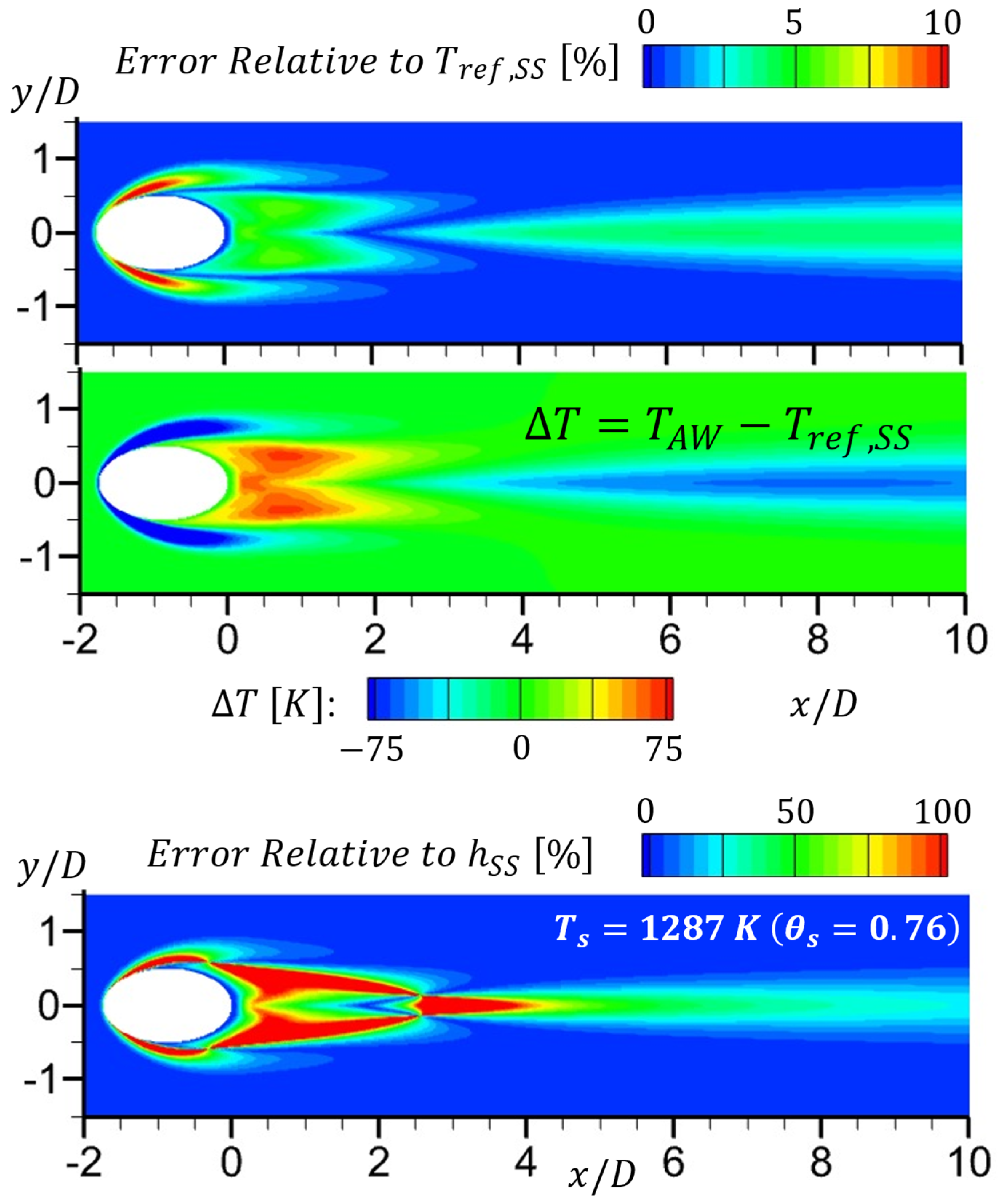
Since the SS method produces a unique T r e f , S S ( x , y ) which ensures that T s T r e f , S S ( x , y ) = 0 , q s ( x , y ) = 0 and a unique h S S (x,y) that is continuous across T s T r e f , S S ( x , y ) = 0 , it can be used to assess errors produced by the AW and LE methods for the film-cooled problem depicted in Figure 2 with an isothermal wall. Figure 18 shows the relative and absolute error in T A W obtained by the AW method with respect to T r e f , S S obtained with N = 5 . Figure 18 also shows the error in h A W relative to h s s with the isothermal temperature on the film-cooled surface set at T s = 1287 K. From this figure, the relative error in T A W can be seen to be less than 10% with the absolute error in temperature up to 75 K. The relative errors in h A W , however, are substantially higher, between 10 % and 70 % , for a significant region about where T s T A W = 0 . At locations where T s T A W = 0 , the error is infinite because h A W = ± . Thus, though the relative error in T A W may be acceptable, the huge errors in h A W should be unacceptable. Results obtained show the size of the region with large errors in h A W to increases as T s increases. This is because the gradient of T A W about where T s T A W = 0 is less steep if T s is closer to T h than T c so that there is larger region where | T s T A W | < ϵ with ϵ being a small number.
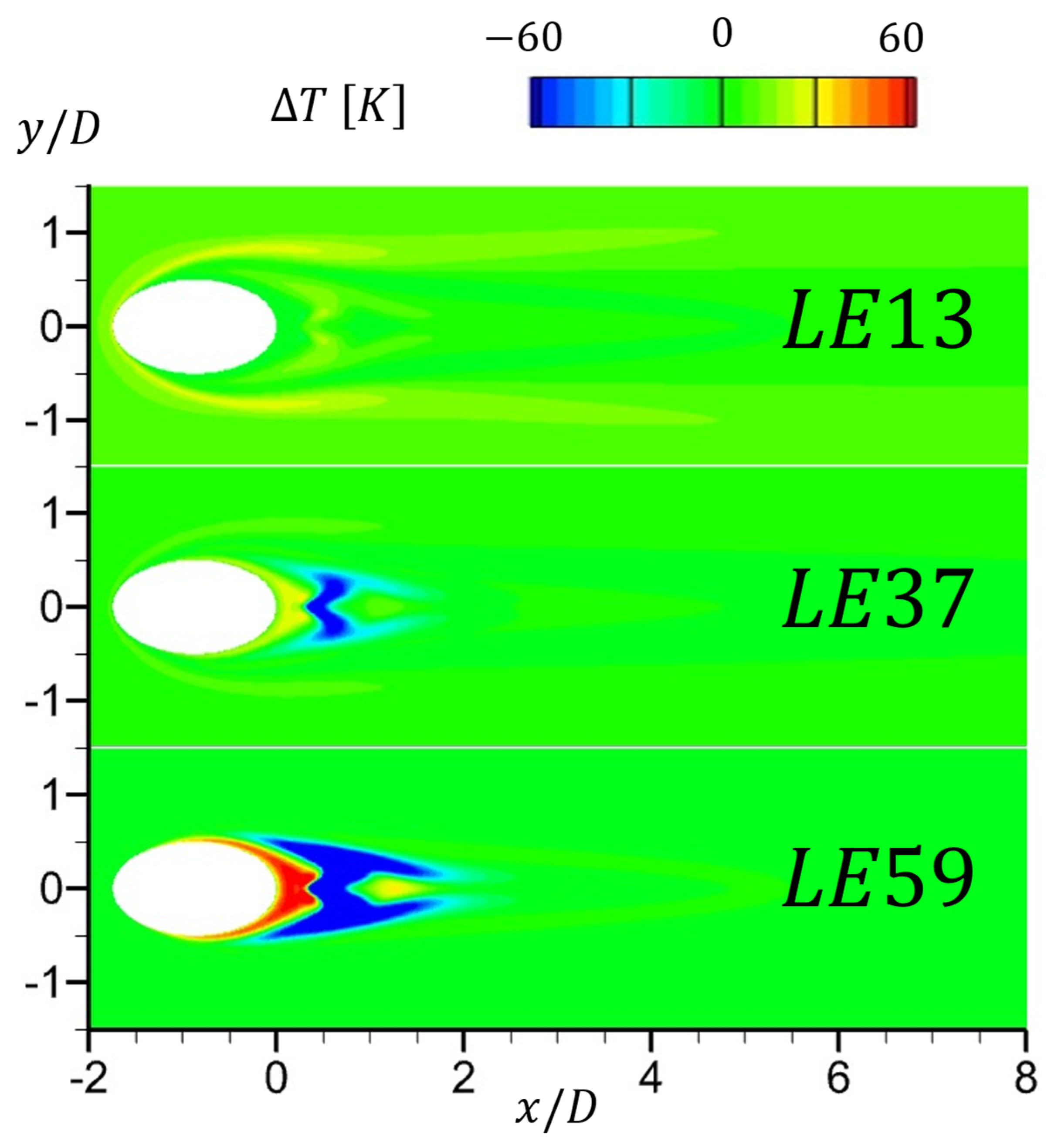
Figure 19 shows the absolute errors in T r e f , L E i j obtained by the LE method with L E i j = L E 13 , L E 37 , and L E 59 relative to T r e f , S S obtained with N = 5 . From this figure, it can be seen that L E i j used in the extrapolation strongly affects T r e f , L E i j . The absolute errors are greatest near the cooling hole because that is where the cooling air first interacts with T s . Thus, errors are minimized if the L E i j used is closer to T c such as L E 13 . However, L E 13 produces the highest absolute error in the region where cooling air interacts with hot air and T s . As shown in Figure 11, if a “wrong” pair of L E i j was chosen such as L E 59 , one could obtain a nonphysical value of T r e f , L E i j   . Thus, choosing appropriate pairs of L E i j is critical for the LE method. Such guidelines have not been developed.
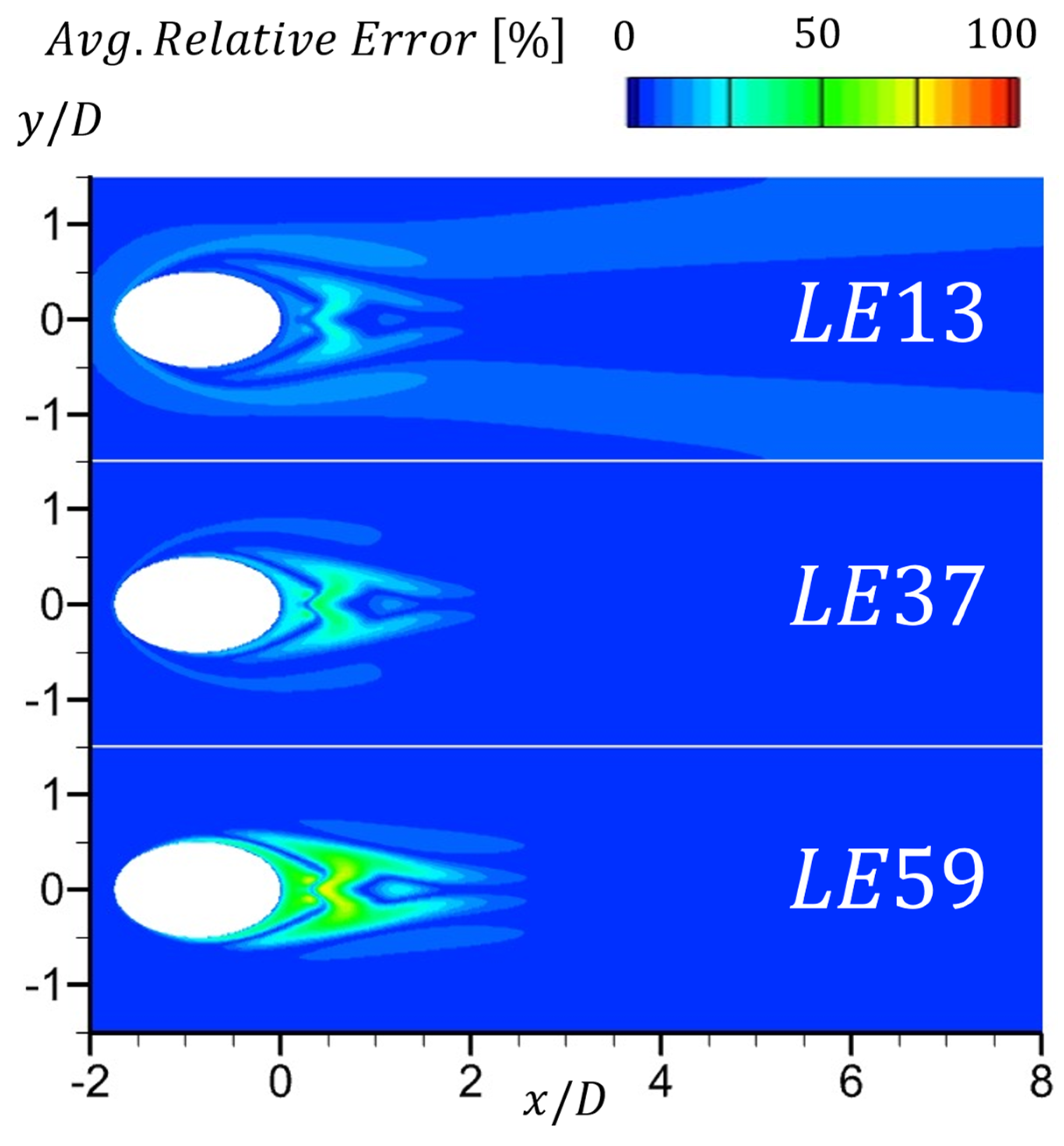
Since the LE method obtains h by assuming that it is independent of T s and the SS method obtains h by accounting for the effects of T s , the error in h L E i j ( x , y ) with respect to h S S ( x , y ) depends on which T s value is used for comparison. For the film-cooled problem shown in Figure 2, T s could be as low as T c to as high as T h . Thus, an “average” relative error in h L E i j measured with respect to h S S ( x , y ,   T s ) is defined as follows:
E h L E i j a v e r a g e = 1 T h T c T c T h E h L E i j d T s = 1 T h T c T c T h h L E i j h S S h S S d T s
Figure 20 shows the average relative error in h L E i j obtained with L E i j = L E 13 , L E 37 , and L E 59 . Similarly to T r e f , L E i j , the errors in h L E i j about the film-cooling hole could be reduced by choosing L E i j pairs that are closer to T c than T h , but the relative error could still be as high as 20 to 40% over a significant portion of the film-cooled surface.

6. Conclusions

This study examined the foundation and the accuracy of three methods for obtaining the reference temperature, T r e f , and the heat-transfer coefficient, h , in Newton’s law of cooling for external flows by using a film-cooling problem where the surface heat transfer, q s , could switch signs: the adiabatic-wall (AW) method, the linear-extrapolation (LE) method, and the state-space (SS) method. This study showed the AW method, which assumes the temperature on an adiabatic wall to be the reference temperature (i.e., T r e f = T A W ), where T s T A W = 0 on the surface, q s does not, in general, equal to zero, so the heat transfer coefficient ( h = h A W ) is infinite where T s = T A W . Though the relative error in T A W may be acceptable (<10%), the relative error in h A W is significant (10–70%) over a substantial portion of the film-cooled surface where T s T A W 0 . For the LE method, which assumes h to depend only the ratio of q s to T s T r e f , L E and independent of T s , the slope of a pair of ( q s ,   T s ) yields h = h L E i j and extrapolation to q s = 0 yields T r e f = T r e f , L E i j . The h L E i j and T r e f , L E i j obtained are not unique with values that depend strongly on the pairs of ( q s ,   T s ) used for extrapolation. The error in T r e f , L E i j and h L E i j can be minimized if the pair of T s , q s used are close to the actual T r e f . However, this is challenging since T r e f could vary from the lowest ( T c ) to the highest ( T h ) temperatures on the film-cooled surface. The state-space method, developed by Peck et al. [43], was the only method that could obtain T r e f = T r e f , S S and h = h S S that are unique, continuous, and meet the requirement where T s T r e f , S S = 0 , q s = 0 . The SS method shows T r e f in Newton’s law of cooling to depend on T s and the corresponding q s of the non-adiabatic wall studied and that using the adiabatic wall or the recovery temperature as T r e f is incorrect. At this point, it is important to emphasize that the errors associated with the AW and LE methods are significant only for convective heat-transfer problems where q s can switch signs, such as in film cooling. This is because the largest errors in h occur about where T S T r e f 0 . For problems where the AW and LE methods provide reasonable T r e f , the SS method can be used to provide error bounds on the computed and measured T r e f and h .

Author Contributions

Conceptualization, T.I.-P.S.; methodology, J.P. and T.I.-P.S.; software, J.P.; validation, J.P.; formal analysis, J.P. and T.I.-P.S.; investigation, J.P. and T.I.-P.S.; resources, K.M.B. and J.M.C.; data curation, J.P.; writing—original draft preparation, T.I.-P.S. and J.P.; writing—review and editing, T.I.-P.S., J.P., K.M.B. and J.M.C.; visualization, J.P.; supervision, T.I.-P.S.; project administration, K.M.B. and T.I.-P.S.; funding acquisition, J.M.C. All authors have read and agreed to the published version of the manuscript.

Funding

This research was funded by the US Department of Energy-Office of Fossil Energy, Advanced Turbines Program under contract no. DE-AC02-07CH11358 through the Ames Laboratory agreement no. 26110-AMES-CMI. The authors are grateful for this support.

Data Availability Statement

The original contributions presented in this study are included in the article. Further inquiries can be directed to the corresponding author.

Conflicts of Interest

The authors declare no conflict of interest.

Nomenclature

C p specific heat at constant pressure
D diameter of film-cooling hole
E i j T s i ,   q s i and T s j ,   q s j pair used in the LE method
H height of computational domain
h heat-transfer coefficient
k thermal conductivity
L i dimensions of the film-cooled flat plate in Figure 2
P static pressure
P r , P r t laminar, turbulent Prandtl number
q s heat flux on surface exposed to convection
S spacing between film-cooling holes
T ,   T c ,   T h temperature, T of cooling air, T of hot air
T A W adiabatic wall temperature
T r e f reference temperature in Newton’s law of cooling
T s temperature on surface exposed to convection
x ,   y ,   z coordinate axes
θ non-dimensional T s : θ = ( T h T s ) / ( T h T c )
μ laminar viscosity
τ shear stress
ϕ film-cooling hole angle with respect to flat plate
ψ variable used to span the state space of T s

References

  1. Kays, W.M.; Crawford, M.E. Convective Heat and Mass Transfer, 2nd ed.; McGraw-Hill: New York, NY, USA, 1980. [Google Scholar]
  2. Goldstein, R.J. Film Cooling. Adv. Heat Transf. 1971, 7, 321–379. [Google Scholar]
  3. Lin, Y.L.; Shih, T. I-P. Film Cooling of a Semi-Cylindrical Leading Edge with Injection through Rows of Compound-Angled Holes. ASME J. Heat Transf. 2001, 123, 645–654. [Google Scholar] [CrossRef]
  4. Nastasi, R.; Rosafio, N.; Salvadori, S.; Misul, D.A. Evaluation of Film Cooling Adiabatic Effectiveness and Net Heat Flux Reduction on a Flat Plate Using Scale-Adaptive Simulation and Stress-Blended Eddy Simuylation Approaches. Energies 2024, 17, 2782. [Google Scholar] [CrossRef]
  5. Ethridge, M.I.; Cutbirth, J.M.; Bogard, D.G. Scaling of Performance for Varying Density Ratio Coolants on an Airfoil with Strong Curvature and Pressure Gradient Effects. ASME J. Turbomach. 2001, 123, 231–237. [Google Scholar] [CrossRef]
  6. Gritsch, M.; Baldauf, S.; Martiny, M.; Schulz, A.; Wittig, S. The Superposition Approach to Local Heat Transfer Coefficient in High Density Ratio Film Cooling Flows; ASME 99-GT-168; ASME: New York, NY, USA, 1999. [Google Scholar]
  7. Popp, O.; Smith, D.E.; Bubb, J.V.; Grabowski, H.C., III; Diller, T.E.; Schetz, J.A.; Ng, T.E. Investigation of Heat Transfer in a Film Cooled Transonic Turbine Cascade, Part I: Steady Heat Transfer; ASME Paper 2000-GT-199; ASME: New York, NY, USA, 2000. [Google Scholar]
  8. Dittmar, J.; Schulz, A.; Wittig, S. Adiabatic Effectiveness and Heat Transfer Coefficient of Shaped Film Cooling Holes on a Scaled Guide Vane Pressure Side Model. Int. J. Rotating Mach. 2004, 10, 345–354. [Google Scholar] [CrossRef]
  9. Pinilla, V.; Solano, J.P.; Paniagua, G.; Anthony, R.J. Adiabatic Wall Temperature Evaluation in a High Speed Turbine. ASME J. Heat Transf. 2012, 134, 091601. [Google Scholar] [CrossRef]
  10. Sousa, J.; Villafane, L.; Paniagua, G. Thermal Analysis and Modelling of Surface Heat Exchangers Operating in the Transonic Regime. Energy 2014, 64, 961–969. [Google Scholar] [CrossRef]
  11. Baldauf, S.; Schulz, S.; Wittig, S. High-Resolution Measurements of Local Heat Transfer Coefficients From Discrete Hole Film Cooling. J. Turbomach. 2001, 123, 749–757. [Google Scholar] [CrossRef]
  12. Eckert, E. Survey on Heat Transfer at High Speeds; WADC Tech Report; Wright Air Development Center, Air Research and Development Command, United States Air Force: Washington, DC, USA, 1954. [Google Scholar]
  13. Sommer, S.C.; Short, B.J. Free-Flight Measurements of Turbulent-Boundary-Layer Skin Friction in the Presence of Severe Aerodynamic Heating at Mach Numbers from 2.8 to 7.0; NACA Technical Note 3391; NACA: Hampton, VA, USA, 1955. [Google Scholar]
  14. van Driest, E.R. The Problem of Aerodynamic Heating. Aeronaut. Eng. Rev. 1956, 15, 26–41. [Google Scholar]
  15. Coles, D.E. The Turbulent Boundary Layer in a Compressible Fluid. Phys. Fluids 1962, 7, 1403–1423. [Google Scholar] [CrossRef]
  16. Higgins, K. Comparison of Engineering Correlations for Predicting Heat Transfer in Zero-Pressure-Gradient Compressible Boundary Layers with CFD and Experimental Data; DSTO Defence Science and Technology Organization: Victoria, OC, Canada, 2008. [Google Scholar]
  17. Neal, L.; Bertram, M.H. Turbulent-Skin-Friction and Heat-Transfer Charts Adapted from the Spalding and Chi Method; NASA-TN-D-3969; NASA: Washington, DC, USA, 1967. [Google Scholar]
  18. Fitt, A.D.; Forth, C.J.P.; Robertson, B.A.; Jones, T.V. Temperature ratio effects in compressible turbulent boundary layers. Int. J. Heat Mass Transf. 1986, 29, 159–164. [Google Scholar] [CrossRef]
  19. Moffat, R.A. What’s New in Convective Heat Transfer. Int. J. Heat Fluid Flow 1998, 19, 90–101. [Google Scholar] [CrossRef]
  20. Arvizu, D.; Moffat, R.J. Use of Superposition in Calculating Cooling Requirements for Circuit Cards Containing Arrays of Electronic Components; Stanford University: Stanford, CA, USA, 1983. [Google Scholar]
  21. Ortega, A.; Moffat, R.J. Heat Transfer from an Array of Simulated Electronic Components: Experimental Results for Free Convection with and without a Shrouding Wall. ASME Heat Transf. Electron. Equip. 1985, 48, 5–15. [Google Scholar]
  22. Anderson, A.; Moffat, R.J. The Adiabatic Heat Transfer Coefficient and the Superposition Kernel Function: Part I—Data for Arrays of Flatpacks for Different Flow Conditions. J. Electron. Packag. 1992, 11, 14–21. [Google Scholar] [CrossRef]
  23. Anderson, A.; Moffat, R.J. The Adiabatic Heat Transfer Coefficient and the Superposition Kernel Function: Part II—Modelling Flatpack Data as a Function of Turbulence. J. Electron. Packag. 1992, 114, 22–28. [Google Scholar] [CrossRef]
  24. Hacker, J.M.; Eaton, J.K. Measurements of Heat Transfer in a Separated and Reattaching Flow with Spatially Varying Thermal Boundary Conditions. Int. J. Heat Fluid Flow 1997, 18, 131–141. [Google Scholar] [CrossRef]
  25. He, L. Spectral Heat Transfer Coefficient for Thermal Design Analysis—Part 1: Augmenting the Cooling Law for Non-Isothermal Wall. ASME J. Turbomach. 2025, 147, 061001. [Google Scholar] [CrossRef]
  26. Incropera, F.P.; DeWitt, D.P. Fundamentals of Heat and Mass Transfer, 5th ed.; John Wiley and Sons: Hoboken, NJ, USA, 2002. [Google Scholar]
  27. Beck, J.V.; St Claire, C.R.; Blackwell, B. Inverse Heat Conduction; John Wiley and Sons: Hoboken, NJ, USA, 2008. [Google Scholar]
  28. Eckert, E.R.; Goldstein, R.J. Measurements in Heat Transfer, 2nd ed.; Hemispshere: Washington, DC, USA, 1976. [Google Scholar]
  29. Han, J.-C.; Dutta, S.; Ekkad, S. Gas Turbine Heat Transfer and Cooling Technology; Taylor and Francis: New York, NY, USA, 2000. [Google Scholar]
  30. Shih, T.I.-P.; Yang, V. (Eds.) Turbine Aerodyanamics, Heat Transfer, Materials, and Mechanics; Progress in Astronautics and Aeronautics; AIAA: Reston, VA, USA, 2014. [Google Scholar]
  31. Ligrani, P.M.; Camci, C. Adiabatic Film Cooling Effectiveness from Heat Transfer Measurements in Compressible, Variable Property Flow. J. Heat Transf. 1985, 107, 313–320. [Google Scholar] [CrossRef]
  32. Camci, C.; Kim, K.; Hippensteele, S.A. A New Hue Capturing Technique for the Quantitative Interpretation of Liquid Crystal Images Used in Convective Heat Transfer Studies. J. Turbomach. 1992, 114, 765–775. [Google Scholar] [CrossRef]
  33. Chyu, M.K.; Ding, H.; Downs, J.P.; Soechting, F.O. Determination of Local Heat Transfer Coefficient Based on Bulk Mean Temperature Using a Transient Liquid Crystal Technique. J. Exp. Therm. Fluid Sci. 1998, 18, 142–149. [Google Scholar] [CrossRef]
  34. Lin, M.; Wang, T. A Transient Liquid Crystal Method Using a 3-D Inverse Transient Conduction Scheme. Int. J. Heat Mass Transf. 2002, 45, 3491–3501. [Google Scholar] [CrossRef]
  35. Owen, J.M.; Newton, P.J.; Lock, G.D. Transient Heat Transfer Measurements Using Thermochromic Liquid Crystal. Part 2: Experimental Uncertainties. Int. J. Heat Fluid Flow 2003, 24, 23–28. [Google Scholar] [CrossRef]
  36. Kassab, A.J.; Divo, E.; Kapat, J.S.; Chyu, M.K. Retrieval of Multi-Dimensional Heat Transfer Coefficient Distributions Using an Inverse-BEM-Based Regularized Algorithm: Numerical and Experimental Examples. Eng. Anal. 2005, 29, 150–160. [Google Scholar]
  37. Bons, J. Transient Method for Convective Heat Transfer Measurement with Lateral Conduction—Part 1: Application to a Deposit-Roughened Gas Turbine Surface. J. Heat Transf. 2009, 131, 011301. [Google Scholar] [CrossRef]
  38. Bons, J.; Fletcher, D.; Borchert, B. Transient Method for Convective Heat Transfer Measurement with Lateral Conduction—Part II: Application to an Isolated Spherical Roughness Element. J. Heat Transf. 2009, 131, 011302. [Google Scholar] [CrossRef]
  39. Nishida, S.; Murata, A.; Saito, H.; Iwamoto, K. Compensation of Three-Dimensional Heat Conduction Inside Wall in Heat Transfer Measurement of Dimpled Surface by Using Transient Technique. J. Enhanc. Heat Transf. 2012, 19, 331–341. [Google Scholar] [CrossRef]
  40. Shih, T.I.-P.; Ramachandran, S.G.; Ames, R.; Dennis, R.A. CFD Conjugate Analysis of Transient Measurements of the Heat-Transfer Coefficient in a Duct with Pin Fins. In Proceedings of the 50th AIAA Aerospace Sciences Meeting including the New Horizons Forum and Aerospace Expo-sition, Nashville, TN, USA, 9–12 January 2012. [Google Scholar]
  41. Shih, T.I-P.; Gomatam-Ramachandran, S.; Chyu, M.K. Time Accurate CFD Conjugate Analysis of Transient Measurements of the Heat-Transfer Coefficient in a Channel with Pin Fins. J. Propuls. Power Res. 2013, 2, 10–19. [Google Scholar] [CrossRef]
  42. Sathyanarayanan, S.K.; Shih, T.I-P. Time-Accurate Conjugate Analysis of Transient Measurements of Heat-Transfer Coefficients. AIAA J. Thermophys. Heat Transf. 2017, 31, 527–537. [Google Scholar] [CrossRef]
  43. Peck, J.; Liu, J.; Bryden, K.M.; Shih, T.I.-P. Method for Measuring and Computing the Adiabatic Wall Temperature; ASME Paper GT2020-14169; ASME: London, UK, 2020. [Google Scholar]
  44. Umana, E.M.; Yang, X. Review of Film Cooling Techniques for Aerospace Vehicles. Energies 2025, 18, 3085. [Google Scholar] [CrossRef]
  45. Kuo, K.K. Principles of Combustion; Wiley: New York, NY, USA, 1986. [Google Scholar]
  46. Bergman, T.L.; Lavine, A.S.; Incropera, F.P.; Dewitt, D.P. Fundamentals of Heat & Mass Transfer, 7th ed.; Wiley: Hoboken, NJ, USA, 2011. [Google Scholar]
  47. Shih, T.-H.; Liou, W.; Shabbir, A.; Zhu, J. A New k ϵ Eddy Viscosity Model for High Reynolds Number Turbulent Flow—Model Development and Validation. Comput. Fluids 1995, 24, 227–238. [Google Scholar] [CrossRef]
  48. Chen, H.C.; Patel, V.C. Near-Wall Turbulence Modles for Complex Flows Including Separation. AIAA J. 1988, 26, 641–648. [Google Scholar] [CrossRef]
  49. Wolfshtein, M. The Velocity and Temperature Distribution in One-Dimensional Flow with Turbulence Augmentation and Pressure Gradient. Int. J. Heat Mass Transf. 1969, 12, 301–318. [Google Scholar] [CrossRef]
  50. ANSYS Inc. Ansys® Academic Research Fluent, Release 2021 R2; Help System, Fluent Theory Guide; ANSYS Inc.: Canonsburg, PA, USA, 2021. [Google Scholar]
  51. Rhie, C.M.; Chow, W.L. Numerical Study of Turbulent Flow Past and Airfoild with Trailing Edge Separation. AIAA J. 1983, 21, 1525–1532. [Google Scholar] [CrossRef]
  52. Uri, M.A.; Grief, C. Chapter 11—Piecewise Polynomial Interpolation. In A First Course in Numerical Computing; Estep, D., Ed.; Society for Industrial and Applied Mathematics: Philadelphia, PA, USA, 2011; pp. 311–359. [Google Scholar]
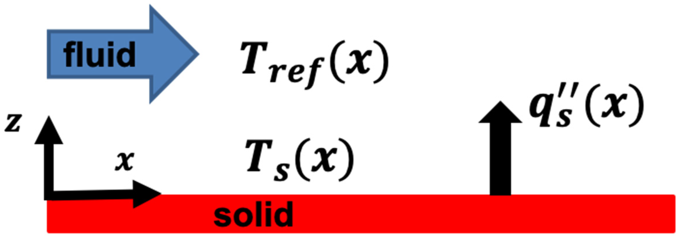
Figure 1. Convective heat transfer over a flat plate.
Energies 18 04074 g001
Figure 2. Schematic of the film-cooling problem studied.
Energies 18 04074 g002
Figure 3. Baseline grid used.
Energies 18 04074 g003
Figure 4. T A W as a function of grid resolution, and error in T A W relative to T A W obtained on the fine grid.
Energies 18 04074 g004aEnergies 18 04074 g004b
Figure 5. q s as a function of grid resolution.
Energies 18 04074 g005
Figure 6. Locations where q s = 0 and where T s T A W = 0 on the film-cooled surface for the three grids used.
Energies 18 04074 g006
Figure 7. Locations where q s = 0 and where T s T A W = 0 on the film-cooled surface as a function of T s .
Energies 18 04074 g007
Figure 8. h A W on the film-cooled surface obtained by the BC method.
Energies 18 04074 g008
Figure 9. Magnitude of shear stress τ s on the film-cooled surface obtained on an adiabatic wall and isothermal wall at x , y = ( D , y ) .
Energies 18 04074 g009
Figure 10. Locations where q s = 0 and where T s T A W = 0 obtained by compressible and incompressible flow formulations at the same T s .
Energies 18 04074 g010
Figure 11. T r e f , L E i j obtained by extrapolating different pairs of ( T s i , q s i ) and ( T s j , q s j ) to q s = 0 with L E i j = L E 15 , L E 37 , and L E 59 .
Energies 18 04074 g011
Figure 12. h L E i j obtained by extrapolating different pairs of ( T s i , q s i ) and ( T s j , q s j ) denoted as L E i j as a function of x , y = ( D , y ) .
Energies 18 04074 g012
Figure 13. q s i as a function of T s i at x , y = D , 0.3 D and at x , y = D , 0.6 D .
Energies 18 04074 g013
Figure 14. q s x , y obtained by using T s ψ i from Set 4 in Table 1.
Energies 18 04074 g014
Figure 15. q s ( x , y ) as a function of T s ( ψ ) and n at x , y = D , 0.3 D obtained in Step 3 of the SS method.
Energies 18 04074 g015
Figure 16. T r e f ( x , y ) and h S S ( x , y ) as a function of N obtained in Steps 4, 5, and 6 of the SS method.
Energies 18 04074 g016
Figure 17. T r e f , S S ( x , y ) obtained with N = 5 and h s s ( x , y ) obtained with T s = 1375 K, a temperature not used to construct G T ψ ,   q s x , y = 0 in Step 3 of the SS method.
Energies 18 04074 g017
Figure 18. Top: Relative and absolute error in T A W ( x , y ) measured with respect to T r e f , S S ( x , y ) obtained with N = 5 . Bottom: Relative error in h A W ( x , y ) measured with respect to h S S ( x , y ) with T S = 1287   K on the film-cooled surface.
Energies 18 04074 g018
Figure 19. Absolute error in T r e f , L E i j with respect to T r e f , S S as a function of different pairs of T s i ,   q s i used.
Energies 18 04074 g019
Figure 20. The average relative error in h L E i j with respect to h S S on the film-cooled surface.
Energies 18 04074 g020
Table 1. Temperatures imposed on isothermal walls.
Set Number T s K
1: AW method ( i = 2 , 3 , 4 , 5 ) 1199, 1287, 1375, 1463
2: LE method ( i = 1 , 3 , 5 , 7 , 9 ) 1112, 1287, 1463, 1638, 1814
3: SS method ( i = 1 , 3 , 9 ) 1112, 1463, 1814
4: SS method ( i = 1 , 3 , 5 , 7 , 9 ) 1112, 1287, 1463, 1638, 1814
5: SS method ( i = 1 , 2 , , 9 ) 1112, 1199, 1287, 1375, 1463, 1550, 1638, 1726, 1814
Table 2. Grids used.
GridTotal No. of Cells (Million)No. of Grid Points on Hole Circumference
coarse1.72112
baseline5.70172
fine20.3264
Disclaimer/Publisher’s Note: The statements, opinions and data contained in all publications are solely those of the individual author(s) and contributor(s) and not of MDPI and/or the editor(s). MDPI and/or the editor(s) disclaim responsibility for any injury to people or property resulting from any ideas, methods, instructions or products referred to in the content.