Abstract
Transpiration cooling that utilizes the phase change of a liquid coolant is recognized as an effective thermal protection technique for extreme environments. However, the introduction of phase change within the porous structure brings about challenges, such as vapor blockage, pressure fluctuations, and temperature inversion, which critically influence system reliability. This study conducts numerical analyses of coupled processes of heat transfer, flow, and phase change in transpiration cooling using a Two-Phase Mixture Model. The simulation incorporates a Local Thermal Non-Equilibrium approach to capture the distinct temperature fields of the solid and fluid phases, enabling accurate prediction of the thermal response within two-phase and single-phase regions. The results reveal that under low heat flux, dominant capillary action suppresses dry-out and expands the two-phase region. Conversely, high heat flux causes vaporization to overwhelm the capillary supply, forming a superheated vapor layer and constricting the two-phase zone. The analysis also explains a paradoxical pressure drop, where an initial increase in flow rate reduces pressure loss by suppressing the high-viscosity vapor phase. Furthermore, a local temperature inversion, where the fluid becomes hotter than the solid matrix, is identified and attributed to vapor counterflow and its subsequent condensation.
1. Introduction
Recent advances in aerospace technology have significantly improved the aerodynamic stability and propulsion performance of hypersonic vehicles, enabling sustained flight at increasingly higher Mach numbers. Nevertheless, to meet the growing thrust requirements associated with these high-speed applications, combustion chambers are required to operate under increasingly severe thermal and pressure conditions. Furthermore, vehicle surfaces are subjected to intense aerodynamic heating due to strong shock waves and viscous dissipation, which result from high-speed flow interactions [1]. In particular, for air-breathing hypersonic vehicles operating at Mach 10, combustor temperature can reach around 3889 K, far surpassing the melting points of current structural materials [2,3]. Therefore, effective and advanced cooling mechanisms are paramount for enabling sustained hypersonic flight.
Among active cooling methodologies, transpiration cooling is consistently recognized as the most thermally efficient approach [4]. The superior cooling efficiency of transpiration cooling is attributed to two synergistic heat transfer mechanisms operating in the porous structure. The first mechanism is manifested in the injection of the coolant into the porous medium. High specific surface area of the solid matrix results in an effective heat exchange with the injected coolants. Simultaneously, the uniform flow distribution maintained within the fine pore channels prevents the formation of hot spots by alleviating local temperature gradients. The secondary mechanism is realized by the thermal barrier effect formed on the surface by the coolant after passing through the porous medium. This continuous coolant layer changes the local temperature and velocity of the boundary layer near the wall, reducing the incoming heat flux. Due to these advantages, transpiration cooling is extensively investigated as a thermal protection technology for diverse aerospace applications, including the combustion chambers of liquid rocket engines [5,6], turbine blades [7,8], and the leading edges of hypersonic vehicles [9,10,11].
The utilization of latent heat from a liquid coolant’s phase change enables a substantial leap in the thermal performance of transpiration cooling. Van foreest et al. [11] performed arc-heated wind tunnel experiments to compare the cooling efficiency of liquid water and nitrogen gas as coolants in transpiration cooling. The results showed that using liquid water at a flow rate of 0.2 g/s reduced the model surface temperature from more than 2000 K to less than 500 K, whereas a fivefold increase in the mass flow rate of nitrogen gas could only reduce the surface temperature to about 1500 K.
Despite these improvements in cooling performance, the onset of phase change within the porous structure introduces inherent challenges, primarily due to the generation of vapor, which has a much higher specific volume than its liquid phase. Under high heat flux conditions, liquid-phase coolant within a confined porous channel rapidly changes to vapor-phase coolant, and the resulting rapid volume expansion impedes a stable coolant supply. Huang et al. [12] experimentally investigated the effects of injection ratio and particle diameter on liquid water transpiration cooling, identifying the vapor-blockage effect as a critical limiting factor. They demonstrated that while reducing particle size from 600 to 200 μm improved cooling, a further reduction to 90 μm dramatically decreased cooling efficiency and increased pressure drop due to vapor-blockage effect. Luan et al. [13] experimentally investigated the instability of liquid transpiration cooling, revealing that under certain conditions, the system enters a periodically fluctuating state instead of reaching a steady state. They attributed this oscillatory behavior, characterized by temperature and pressure variations, to the complex interplay between capillary forces and the severe phase-change process within the pores.
The key limitation of these experiments is the inability to see inside the porous material. These uncertainties about internal flow and phase changes pose obstacles to the design of reliable systems for practical use. Therefore, theoretical and numerical approaches that can overcome these experimental limitations and quantitatively characterize the phase change, and heat transfer mechanisms are required to ensure reliability and maximize the performance of liquid transpiration cooling systems. Mathematical modeling of phase change in porous media is typically approached through Separated Phase Models (SPMs) [14,15,16] and Two-Phase Mixture Models (TPMMs) [17,18,19,20]. While SPMs accurately describe multiphase flow by solving distinct sets of conservation equations for each phase, this approach is computationally expensive as it necessitates complex interface tracking and the solution of coupled nonlinear equations. To overcome these limitations, the TPMM proposed by Wang and Beckerman [17] has been modified and developed in various forms in recent years. In contrast to SPMs, TPMMs treat the liquid and gas as a single continuous fluid with averaged properties, such as mixture density, pressure, and velocity. This approach allows the three sets of conservation equations used in SPMs to be reformulated into a single, unified mathematical expression. Wang [18] proposed a new enthalpy formulation to eliminate the tendency of non-monotonic variation of mixture enthalpy in conventional TPMMs to simulate boiling. Hu et al. [19] conducted a numerical study to investigate flow boiling phenomena in porous media. Their model, based on the TPMM, introduced the concept of kinetic enthalpy to handle nonlinear advection terms and ensure numerical stability. However, they did not account for LTNE (local thermal non-equilibrium) characteristics in their analysis.
Furthermore, Shi and Wang [20] proposed a Local Thermal Non-Equilibrium and Two-Phase Mixture Model (LTNE–TPMM) that considers the heat exchange between solid and fluid in the pores. Based on the modified model, they analyzed the effects of coolant mass flow rate, heat flux, thermal conductivity, porosity, particle diameter, and saturation pressure on the distribution of temperature and liquid saturation. The fundamental contrast between the Local Thermal Equilibrium (LTE) and Local Thermal Non-Equilibrium (LTNE) assumptions for modeling phase change was systematically investigated by Ray and Alomar [21]. Their numerical study concluded that the widely used LTE model is fundamentally flawed for this application, as it produces unrealistically high wall temperatures and fails to capture the expansion of the superheated vapor region. They demonstrated that the more complex LTNE model, which accounts for separate solid-phase conduction and internal heat exchange, is essential for obtaining physically realistic predictions. Marafie and Vafai [22] conducted an analytical study of forced convection flow through channels filled with porous media using the Darcy–Forchheimer–Brinkman model coupled with a two-equation model that accounts for local thermal non-equilibrium. Their analysis systematically incorporated the effects of key dimensionless parameters such as the Biot number, thermal conductivity ratio, Darcy number, and inertia parameter. They found that as the disparity in thermal conductivity between the solid and fluid phases increases, and as the solid phase becomes more thermally dominant, the prediction error associated with the single-equation model increases significantly.
While several studies have addressed specific aspects of phase change and heat transfer in porous structures, there remains a need for comprehensive analyses that elucidate the fundamental physical mechanisms and systematically explore the effects of key variables such as coolant flow rate and heat flux. In this study, a numerical model based on the LTNE–TPMM framework is developed to investigate the phase-change phenomena, as well as the corresponding pressure drop and temperature characteristics, in transpiration cooling. Numerical convergence is enhanced by applying a smoothing technique using the kinetic enthalpy concept, which mitigates the occurrence of unphysical jumps in the fluid energy equation. To validate the new model, single-phase experiments were conducted using in-house fabricated specimens, and further comparative analysis with published results allowed extension of the model’s applicability to multiphase regimes. With the validated model, the interrelationships among phase-change location, thickness, temperature field, and pressure drop were systematically examined for two representative heat flux cases across a range of coolant mass flux conditions. The analysis results showed a unique negative pressure gradient in which pressure decreased as flow rate increased due to high flow resistance caused by the vapor phase during the phase-change process. In addition, a detailed discussion of the velocity and temperature fields at the phase-change interface was conducted, highlighting the temperature inversion phenomenon and offering new insights into the underlying heat and flow mechanisms.
2. Mathematical Model and Numerical Methodologies
2.1. Modified LTNE–TPMM
The mathematical description of the two-phase flow and heat transfer within the porous medium is based on the Two-Phase Mixture Model (TPMM) framework, originally proposed by Wang and Beckermann [17]. In its foundational form, the model consists of conservation equations for mass, momentum, and energy. The conservation of mass for the two-phase mixture is given by
The momentum conservation of the mixture, which describes the relationship between pressure drop and fluid momentum in porous media, is governed by Darcy’s law. In its complete form, including the gravitational body force, the momentum equation is given as
However, in the present study, the gravity term is omitted from the momentum equation. This simplification is reasonable as the influence of gravity is negligible compared to the dominant Darcy viscous resistance. To support this quantitatively, an order-of-magnitude analysis was conducted. For representative flow conditions in this study, the Darcy resistance term is on the order of 105 N/m3, whereas the gravity term is only on the order of 103 N/m3. This result was further validated by a numerical sensitivity analysis for the case where the fluid in the porous medium is a fully saturated liquid. The results showed that the inclusion of gravity increased the total pressure drop from 4108.41 Pa to 4183.74 Pa, corresponding to a change of only 1.8%. Therefore, the simplified momentum equation used in this study is given as
In its original formulation, the TPMM often employs the Local Thermal Equilibrium (LTE) assumption for energy conservation. This approach simplifies the thermal analysis by using a single energy equation, which presumes a unified temperature field for the solid, liquid, and vapor phases. This single energy equation is typically expressed as
In this LTE formulation, keff represents a volume-averaged effective thermal conductivity of the saturated porous medium, and T is a single, unified temperature shared by the solid matrix, the liquid water, and its vapor, and Q is the energy source term.
However, the LTE approach has two fundamental limitations in situations where it is exposed to high heat fluxes, as investigated in this study. Firstly, the LTE model’s single effective thermal conductivity is inaccurate, as it is derived by averaging the properties of solids and fluids. The thermal conductivity of the gas phase is many orders of magnitude lower than the thermal conductivity of the liquid and solid phases. Averaging these vastly different values can physically overestimate the heat transfer in vapor-dominated regions and incorrectly predict the temperature field. Second, in the two-phase region, the LTE assumption is physically untenable. During the vaporization, the fluid must be constant at its saturation temperature, while the solid porous matrix undergoes temperature changes due to external heat fluxes. The LTE model, by enforcing a single temperature for both phases, is fundamentally incapable of representing this temperature difference.
To address this critical deficiency, the present study adopts the Local Thermal Non-Equilibrium (LTNE) approach, building upon the model developed by Shi and Wang [19]. The single energy equation of the LTE model is replaced by two separate energy conservation equations for the solid and the fluid. This LTNE approach allows each phase to have its own temperature field, thereby capturing the temperature difference that drives the boiling process. To achieve this, the model’s single effective thermal conductivity (keff) is split into distinct conductivities for the solid (ks, eff) and the fluid (kf, eff). Furthermore, the heat exchange between the superheated solid wall and the saturated fluid is no longer a generic source term but is explicitly modeled by an interfacial heat transfer term (qsf). This term directly couples the two energy equations, acting as a heat sink for the solid phase and a corresponding heat source for the fluid phase. Consequently, the energy conservation equation for fluid and solid in the steady-state LTNE–TPMM can be expressed by modifying Equation (3):
Equation (4) consists of four terms—the advection term on the left side of the equal sign, and three terms on the right side representing energy diffusion by heat conduction, energy diffusion by capillary-induced mass flux, and the solid–fluid volumetric heat source, respectively. The separation of advection and capillary diffusion terms is necessary because the original advection term, , implicitly combines two distinct physical effects: energy transport by bulk fluid mixture motion and energy transport due to relative motion between individual phases. By reformulating this complex term in terms of fluid mixture enthalpy, Equation (4) explicitly distinguishes these two mechanisms, preserving the essential physics of two-phase energy transport.
The use of traditional mixture enthalpy as the primary variable in the energy equation suffers from numerical stiffness during phase change. A small increment in enthalpy within the two-phase region can induce a near-vertical drop in density and discontinuous jumps in other properties. In addition, the advection coefficient also includes a denominator term that is nonlinear for fluids in phase change, driven by changes in physical properties and saturation [19,23,24]. As a consequence, steep nonlinear changes in thermal properties occur at the phase boundaries, leading to severe oscillations in residuals and an increase in the number of iterations required for convergence. To resolve these fundamental issues, this study employs a kinetic enthalpy formulation, originally introduced by Wang and Beckermann [17], as shown in Equation (6):
The main advantage of this reformulation is that it provides a continuous and physically stable property profile. For example, density becomes a monotonic and smooth function of enthalpy, changing gradually instead of with a sharp decrease. By ensuring that the property slope remains finite, the formulation effectively linearizes the system’s response to phase changes. In addition, by keeping the coefficient of the advection term of the energy equation as the mass flux (ρu), the computational process of the numerical model can be stabilized [23,24].
Effective diffusion coefficient is defined based on two distinct conditions: in the single-phase regions and in the two-phase region. This leads to the following formulation:
The constitutive relations used in Equations (1), (2), (4), (5), and (6) are described in detail in Appendix A. The thermodynamic properties of the coolant (liquid and vapor) and solid matrix are listed in Table 1 and Table 2, respectively. According to the constitutive relationship shown in Table A1 and the definition of kinetic enthalpy, the relative mobility and liquid saturation are calculated as follows:

Table 1.
Thermodynamic properties of the coolant used in numerical simulations.
Table 2.
Physical properties of the porous structure used in numerical simulations.
2.2. Boundary Conditions
The boundary conditions of the numerical analysis model are applied to the hot side and the cold side of the porous plate. Assuming that the heat flux applied to the hot side of the porous plate is completely absorbed by the solid matrix according to Su et al. [9], the boundary conditions are defined as follows:
The boundary conditions for the cold side of the porous plate are defined as follows by energy conservation, considering the coolant reservoir and convection at the bottom of the porous plate:
where and are the convective heat transfer coefficient at the cold side and the coolant injection temperature, respectively.
2.3. Physical Model
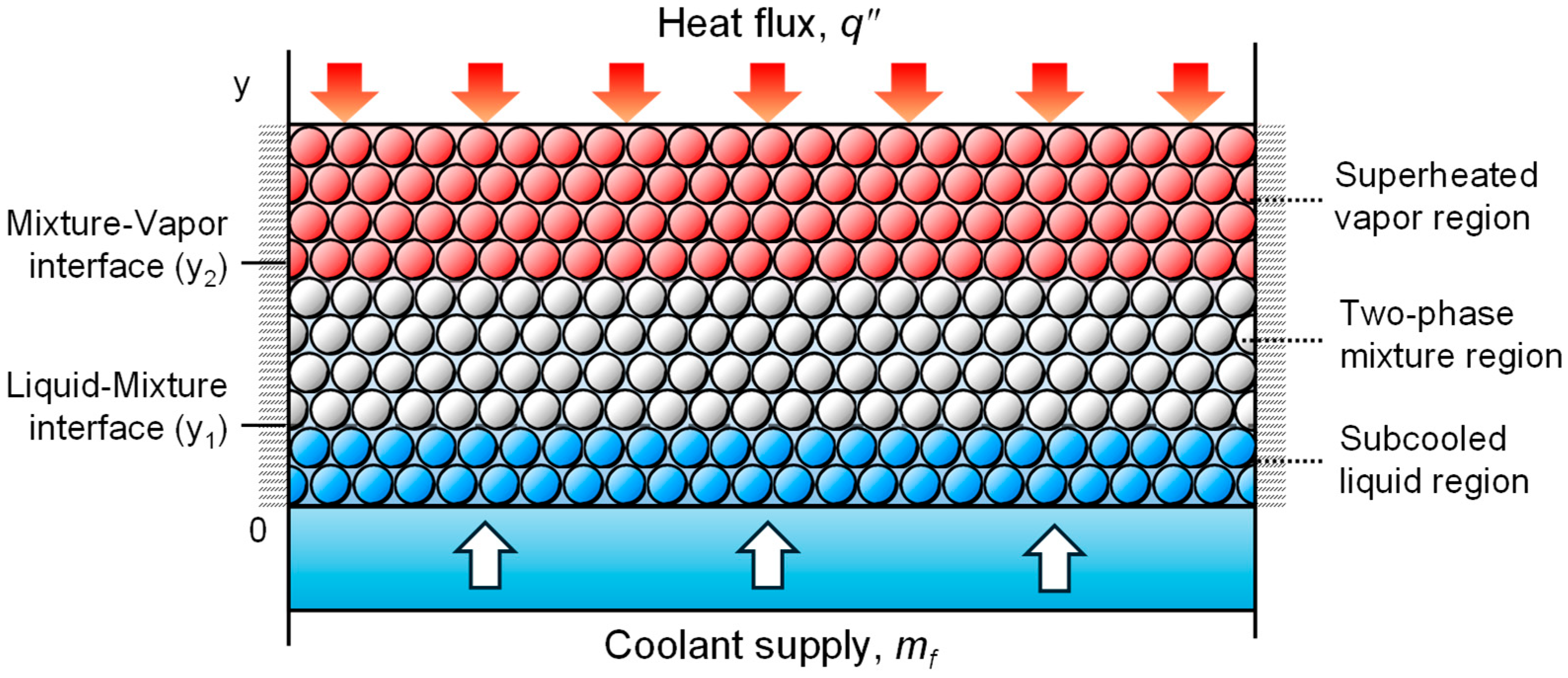
Figure 1 illustrates the physical model employed for the numerical analysis of transpiration cooling in this study. Heat flux is uniformly applied to a region with a diameter of 60 mm (D) through a cylindrical porous plate with a thickness of 8 mm (L). The numerical domain consists of a two-dimensional representative cross-section of the porous plate, assuming macroscopically uniform flow and thermal fields. Wall boundary conditions are applied to the sides of the domain. The plate is composed of Hastelloy X, an Ni-based superalloy known for its high-temperature strength and excellent oxidation resistance. To thermally protect the porous structure, DI water at 300 K is injected at a constant mass flux in a direction opposite to the applied heat flux. The water inside the pores absorbs heat and is vaporized, resulting in three distinct regions inside the porous structure: a subcooled liquid region, a two-phase mixture region, and a superheated vapor region. Depending on the applied heat flux and coolant mass flux, the location of the interface where the phase change occurs is shifted, while the boundary between the liquid and mixture region is denoted as y1, and the boundary between the mixture and vapor region is denoted as y2.

Figure 1.
Schematic diagram of physical model of transpiration cooling with liquid coolant phase change.
2.4. Computational Process
The numerical simulations were performed using the commercial software ANSYS Fluent 2022 R1, which is based on the Finite Volume Method (FVM). To implement the physics of phase-change transpiration cooling, the governing equations and constitutive relations were integrated into the solver through User-Defined Functions (UDFs). The continuity and momentum equations within the porous domain were solved using Fluent’s built-in porous media model, while the energy conservation equations for both the solid and fluid phases were implemented as User-Defined Scalar (UDS) transport equations. Considering the low mass flow rate and small characteristic length that are characteristic of transpiration cooling, the Reynolds number is sufficiently low, making it reasonable to use the laminar flow model. The SIMPLE algorithm was employed for pressure–velocity coupling. For spatial discretization, a second-order upwind scheme was applied to the momentum and energy equations to ensure high accuracy, while the PRESTO! scheme was used for the pressure term.
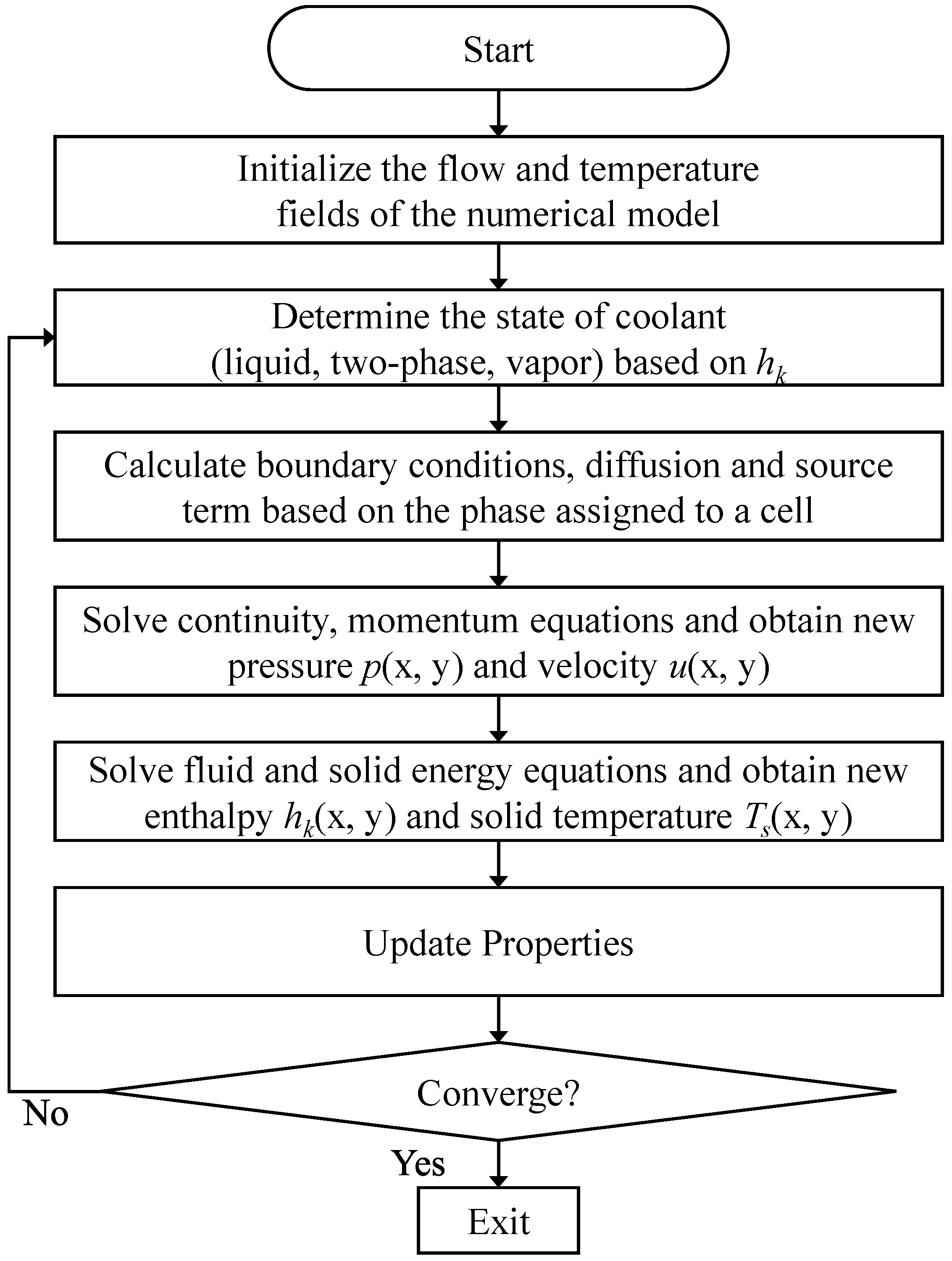
Figure 2 illustrates the iterative computational procedure employed in this study. Initially, to ensure a stable startup, the entire computational domain was initialized with the velocity profile from the inlet boundary and a uniform reference temperature of 300 K. Within each iteration, the state of the coolant (liquid, two-phase, or vapor) is first determined for each cell based on the local enthalpy and pressure. Subsequently, all relevant mixture properties, source terms, and constitutive relations are updated to User-Defined Memory (UDM) according to the determined phase. The continuity and momentum equations are then solved to obtain new pressure and velocity fields, followed by the solution of the fluid and solid energy equations to yield updated kinetic enthalpy and solid temperature values. This entire iterative process is repeated until the convergence criteria are met. The convergence criteria were set to 10−6 for continuity and momentum, and 10−8 for energy.

Figure 2.
Flowchart of numerical simulation procedure.
3. Results and Discussion
3.1. Grid Independence Test
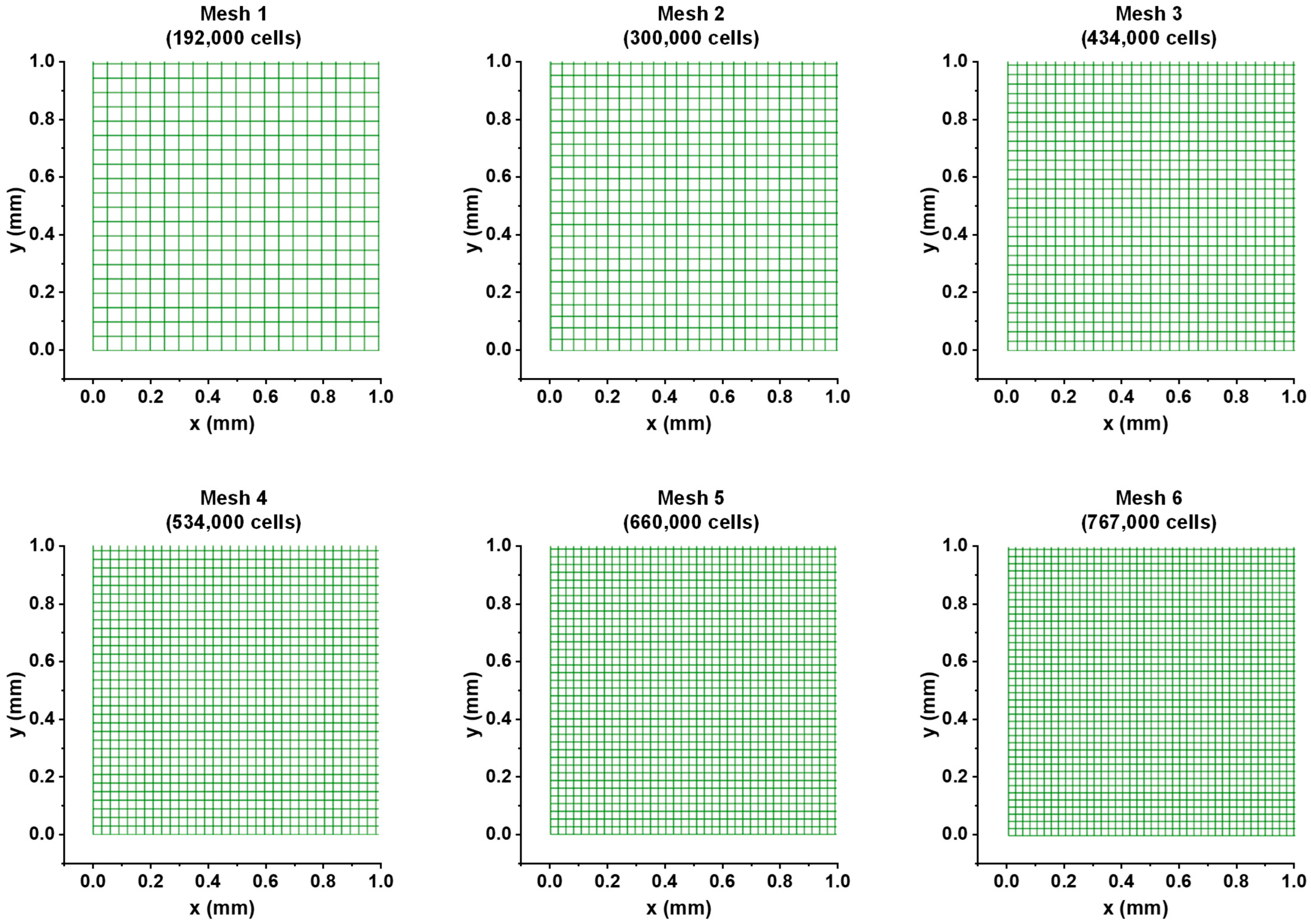
Since the numerical model consists of a simple rectangular domain, a structured computational grid is generated using ICEM CFD for the simulation. Figure 3 shows enlarged views of 1 mm × 1 mm regions for each mesh used in the grid independence test. Although the advection term of the fluid energy equation was smoothed, large temperature gradients and abrupt property changes still occurred near phase-change interfaces, necessitating a high-resolution mesh to accurately capture these sharp variations and ensure the fidelity of simulation results.
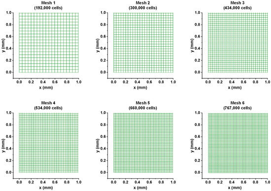
Figure 3.
The enlarged views of the six meshes used for the grid independence test in this numerical study.
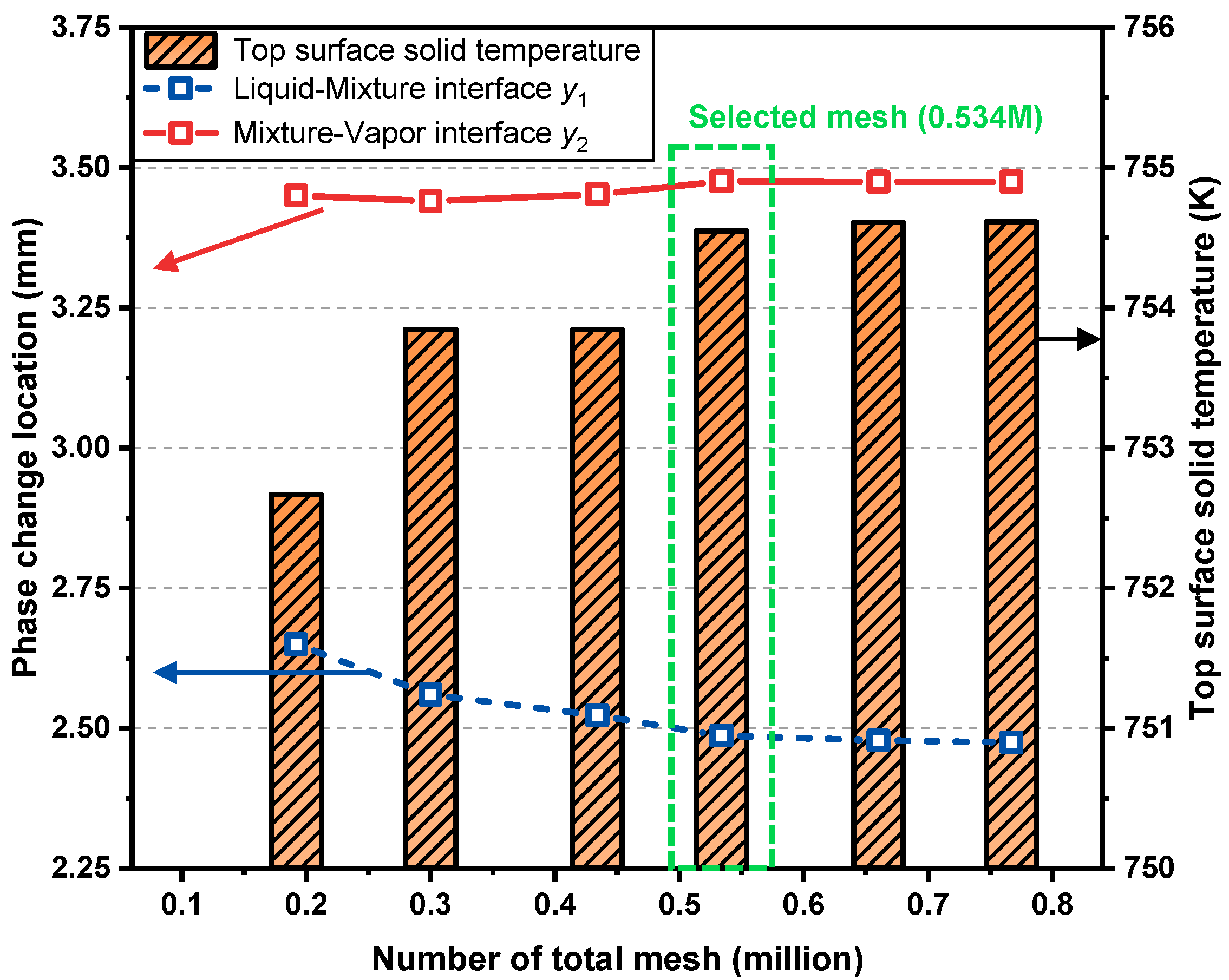
To determine an optimal grid that balances solution accuracy with computational cost, a grid independence study was conducted on six different mesh configurations. In this study, the structured grid is refined by adjusting the element size to 50, 40, 35, 30, 27.5, and 25 μm, which incrementally increased the total cell count from 0.192 million to 0.767 million. The convergence of the solid temperature on the hot-side surface and the positions of the phase-change interfaces are then analyzed. Figure 4 illustrates the grid independence study. An appreciable difference of approximately 6.0% in the thickness of the phase-change region is observed when refining the mesh from 0.434 million to 0.534 million cells. However, further refinement to 0.66 million cells yields a substantially small change of just 0.78% for the same parameter, with the solid temperature varying by only 0.1 K. Consequently, a mesh with 0.534 million cells was selected for the present study.
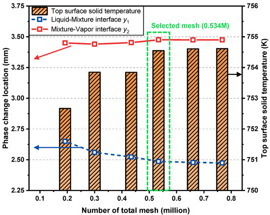
Figure 4.
Comparison of the top surface fluid temperature and phase-change location obtained by six different meshes.
3.2. Numerical Model Validation
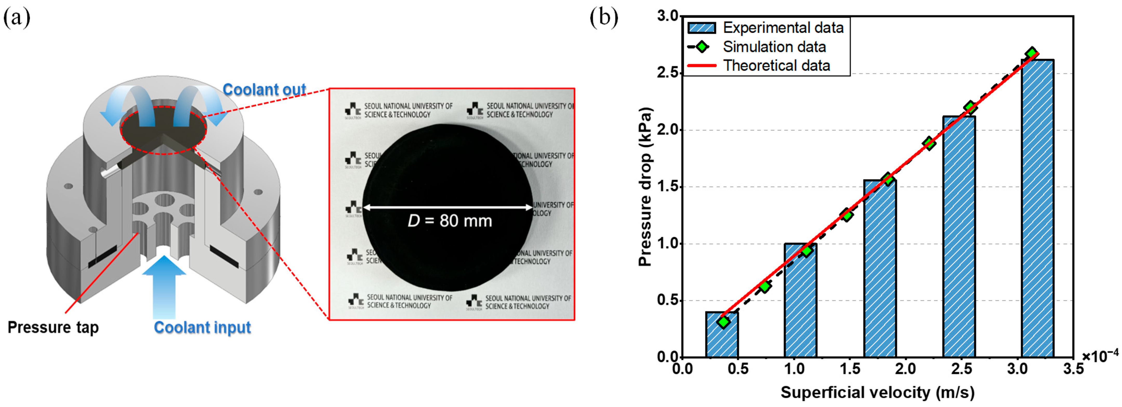
The permeability of the porous specimen is quantified using an experimental setup [25] that allows the measurement of the pressure difference across the top and bottom of the specimen at different flow ranges, as shown in Figure 5a. The test apparatus clamps the specimen with a 10 mm distance from its outer perimeter to the inside, exposing a central discharge area equivalent to a 60 mm diameter. DI water maintained at a constant temperature of 300 K using a chiller (HTRC, JEIO TECH, Daejeon, Republic of Korea) is injected through a plenum inlet located 70 mm above the bottom of the specimen. A two-head piston pump (Intelligent SS, FLOM, Tokyo, Japan) is used to inject water into the specimen over a range of superficial velocities, while a pressure sensor (PSH, SENSYS, Ansan-Si, Republic of Korea) is installed to measure the pressure drop of water across the specimen.
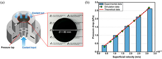
Figure 5.
(a) Schematic diagram of experimental setup. (b) Comparison of numerical results with experimental and theoretical data.
Figure 5b shows the experimentally measured pressure drop over a range of superficial velocities of injected water, along with the theoretical predictions from Darcy’s law and the pressure results from numerical simulations. As shown in Figure 5b, the measured pressure drop has an almost linear relationship with the superficial velocity, which is characteristic of the Darcy flow regime. The permeability of the specimen was extracted by fitting the data to the Darcy equation. The numerical model, employing identical geometry and boundary conditions as the experiment, showed excellent agreement with both experimental and theoretical values. The maximum pointwise deviation between simulation and experimental results was only 90 Pa, and the overall average relative error was 6.7%, thereby validating its predictive capability.
Furthermore, to verify the reliability of the present numerical model in the phase-change region, its results were compared with those from previous studies by Shi and Wang [20] and Chen et al. [26]. The validation case is based on a porous matrix with a thickness of 0.01 m, a porosity of 0.3, and a mean particle diameter of 20 μm. A constant heat flux of 1.0 MW/m2 is applied to the upper side, while coolant with a mass flux of 0.5 kg/m2⋅s is injected from the lower side. Figure 6 compares the fluid temperature distribution along the flow direction predicted by the current model against the results from the aforementioned literature. The comparison demonstrates that the results of the present model are in excellent agreement with the overall temperature trends of the previous studies. The largest relative error was observed at the interface between the liquid and mixture regions. At this location, the present model shows relative errors of 9.4% and 2.74% compared to the results of Shi and Wang [20] and Chen et al. [26], respectively. Overall, despite these localized deviations, the agreement is considered excellent, thus confirming the validity of the present numerical model.
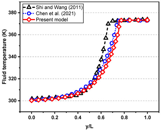
Figure 6.
Comparison of temperature distributions along the flow direction between the present model and the results from previous studies [20,26].
3.3. Flow Regimes and Liquid Saturation Field
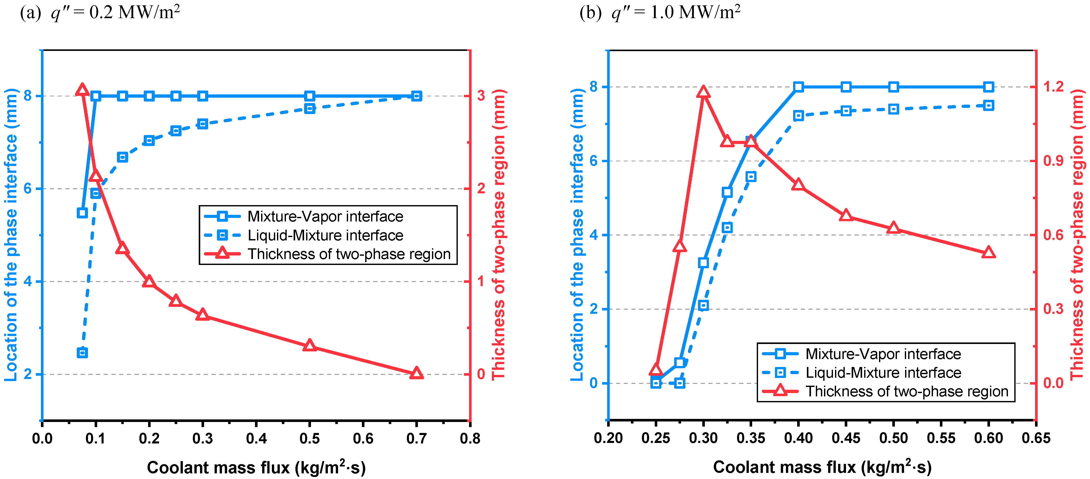
Figure 7 quantitatively illustrates the evolution of the phase-change regime within the porous structure by depicting the locations of the liquid–mixture (y1) and mixture–vapor (y2) interfaces, along with the resulting thickness of the two-phase region, under varying coolant mass flow rates and two distinct heat flux conditions. Generally, a transition from an all-liquid regime occurs as the coolant injection rate is reduced, leading to the local onset of phase change and the formation of a two-phase layer. While this layer’s position and thickness initially remain relatively stable, they undergo a dramatic transformation once the flow rate drops below a critical threshold, a behavior that is highly dependent on the applied heat flux. Under low heat flux conditions (q″ = 0.2 MW/m2), as detailed in Figure 7a, the phase change initiates at a comparatively low flow rate (<0.70 kg/m2⋅s), marked by the penetration of the liquid–mixture interface (y1) from the hot side into the structure. A notable characteristic in this regime is the effective suppression of complete vaporization. Even as the flow rate is greatly decreased down to 0.10 kg/m2·s, the mixture–vapor interface (y2) remains fixed to the hot surface. This results in the progressive expansion of the two-phase region’s thickness. This phenomenon can be interpreted because of the lower thermal load. The heat conducted into the solid matrix is insufficient to vaporize the entire volume of coolant being supplied by capillary action, allowing a substantial portion to remain in a two-phase state. In contrast, under high heat flux conditions (q″ = 1.0 MW/m2), Figure 7b reveals a markedly different behavior. Here, a superheated vapor region begins to form at the hot surface at a much higher flow rate threshold (<0.40 kg/m2⋅s), indicating a greater demand for coolant to manage the intense thermal load. Concurrently, the two-phase region is observed to be relatively narrower compared to the low heat flux case. This constriction suggests a shift in the dominant heat transfer mechanisms. At higher thermal loads, the aggressive incoming heat flux promotes rapid and complete vaporization, where convective and conductive heat transfer dominate over the capillary-driven liquid supply, thus limiting the spatial extent of the two-phase zone.
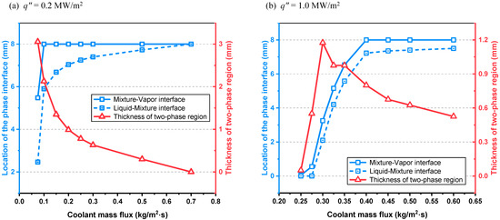
Figure 7.
The variations in location of the phase-change interfaces and thickness of the two-phase region at different coolant mass fluxes under (a) q″ = 0.2 MW/m2 and (b) q″ = 1.0 MW/m2.
3.4. Pressure Drop Characteristics
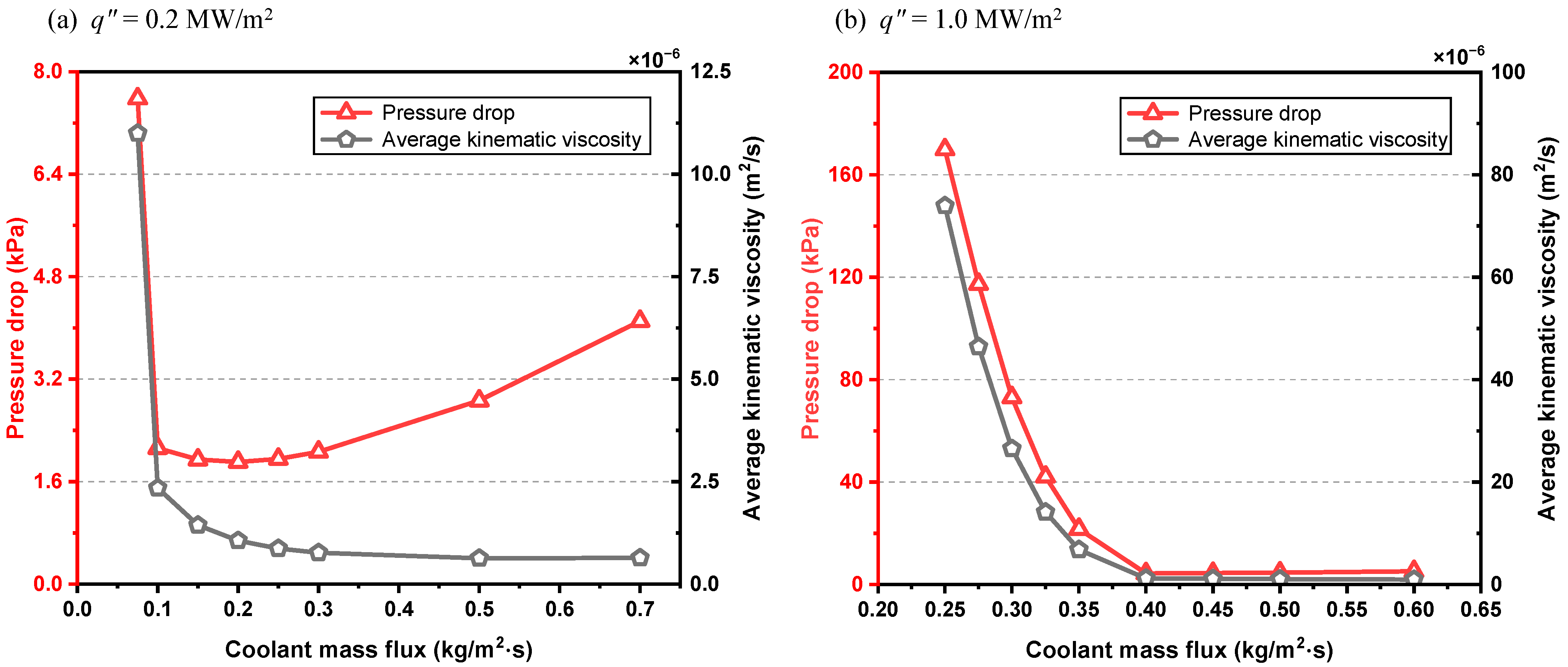
Figure 8 presents the total pressure drop across the porous plate and the corresponding average kinematic viscosity of the coolant as a function of the coolant mass flux. The results reveal a clear transition point where the behavior of both variables changes sharply, and this transition is fundamentally governed by the underlying phase distribution within the porous medium, as shown in Figure 7.
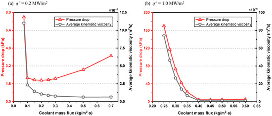
Figure 8.
The variations in pressure drop and average kinematic viscosity at different coolant mass fluxes under (a) q″ = 0.2 MW/m2 and (b) q″ = 1.0 MW/m2.
Before the transition point at low flow rates, both the pressure drop and the average kinematic viscosity decrease markedly with increasing mass flow rate. This behavior is due to the phase distribution caused by vaporization of the fluid in the porous material. As the coolant flow rate increases, vapor generation is suppressed, which in turn significantly reduces the vapor fraction within the mixture. Since the kinematic viscosity of vapor is much higher than that of liquid, this reduction in vapor content results in a substantial decrease in the overall average kinematic viscosity. According to Darcy’s law (Equation (2b)), the pressure drop is proportional to both mass flux and kinematic viscosity. However, in this region, the rapid decrease in average kinematic viscosity due to decreasing vapor fraction outweighs the effect of increasing mass flow rate. As a result, the system exhibits a counterintuitive negative pressure gradient phenomenon, where the pressure drop decreases as the flow rate increases.
This negative pressure slope is characteristic of the so-called Ledinegg instability, which can arise in systems undergoing phase change in porous media and microchannels [27]. The Ledinegg instability is typically associated with an N-shaped relationship in the pressure drop versus mass flow rate curve; when the system operating point falls within the negatively sloped region, it becomes susceptible to sudden flow and pressure instabilities. Therefore, the identification of a negative slope in this analysis is significant in identifying the physical basis of the unexpected pressure characteristic. Furthermore, it highlights the potential dangers of instability that can threaten the safe and reliable operation of phase-change cooling systems.
Conversely, in the region after the transition point at higher flow rates, the system is predominantly filled with the liquid phase. Here, the average kinematic viscosity becomes nearly constant and lower, as shown in Figure 8. Consequently, the influence of kinematic viscosity becomes secondary, and the pressure drop reverts to a more intuitive behavior, increasing almost linearly with the mass flux. However, this regime is inefficient as it requires a large coolant supply while simultaneously generating higher pressure drops, which could negatively impact the coolant delivery system.
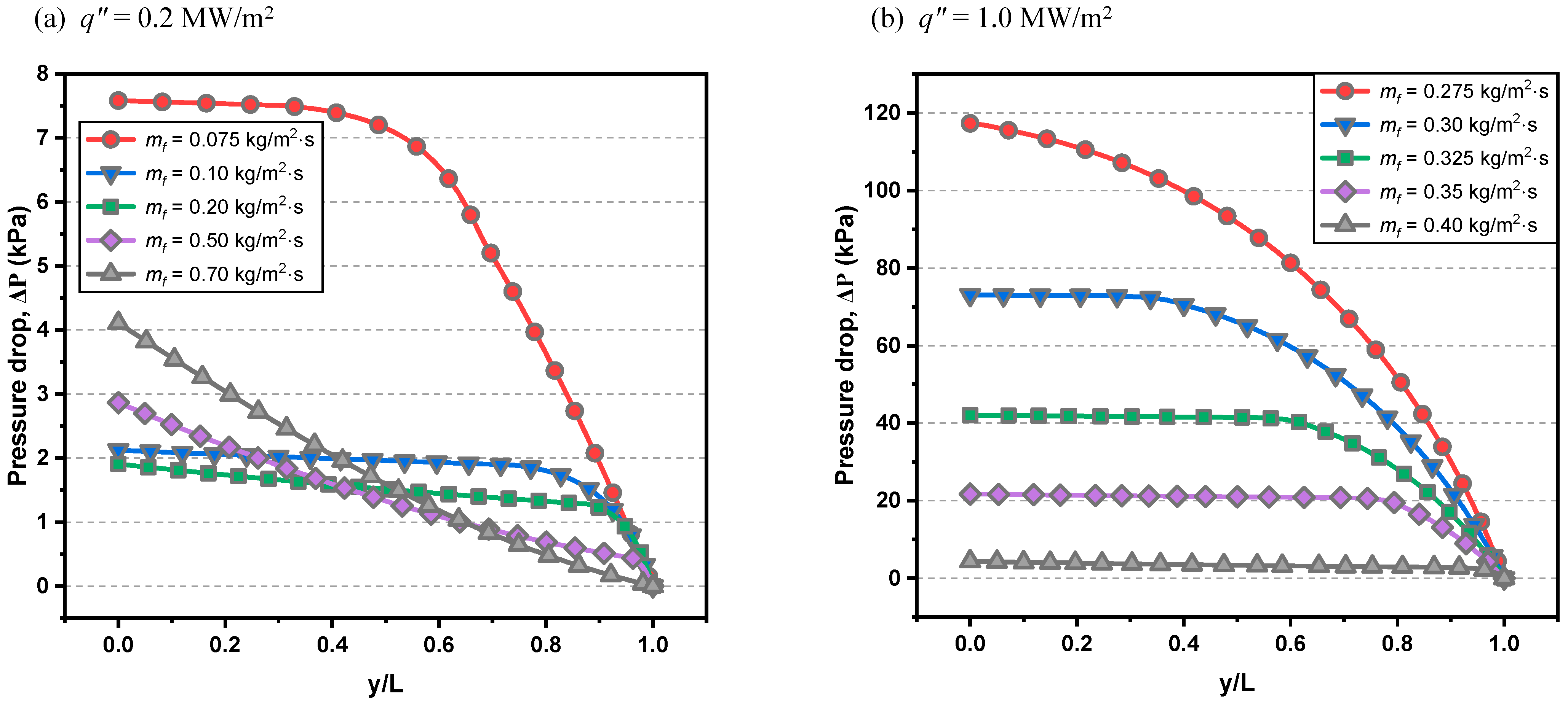
To further elucidate these macroscopic trends, Figure 9 presents the local pressure distribution along the flow direction for representative flow rates. In most cases, the pressure gradient is initially moderate within the single-phase liquid region near the inlet. Downstream, as phase change occurs, the formation of vapor with high kinematic viscosity and two-phase mixture leads to a steep increase in the local pressure gradient, which explains the overall pressure drop behavior observed in Figure 8. This effect is particularly pronounced at lower flow rates, where higher fluid temperatures at the outlet result in higher local vapor viscosity, further steepening the pressure gradient in that region. A final notable feature is observed in the pressure distributions for the highest flow rates of 0.50 and 0.70 kg/m2·s. These cases exhibit a steeper initial pressure gradient compared to some lower flow rate cases. This contrasting result is attributed to the temperature-dependent kinematic viscosity of the liquid water. The high coolant flow rate effectively suppresses the temperature at the inlet, and according to the properties of water, this lower temperature increases its kinematic viscosity. As Darcy’s law dictates that pressure drop is proportional to both viscosity and mass flux, this elevated viscosity of the cold liquid becomes the dominant factor responsible for the steeper initial pressure gradient observed in the all-liquid zone.
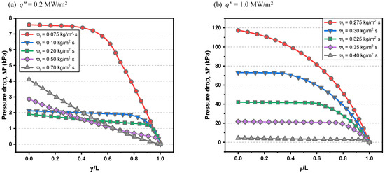
Figure 9.
Pressure distributions along flow direction at different coolant mass fluxes under (a) q″ = 0.2 MW/m2 and (b) q″ = 1.0 MW/m2.
3.5. Analysis of Temperature Field and Local Thermal Non-Equilibrium Characteristics
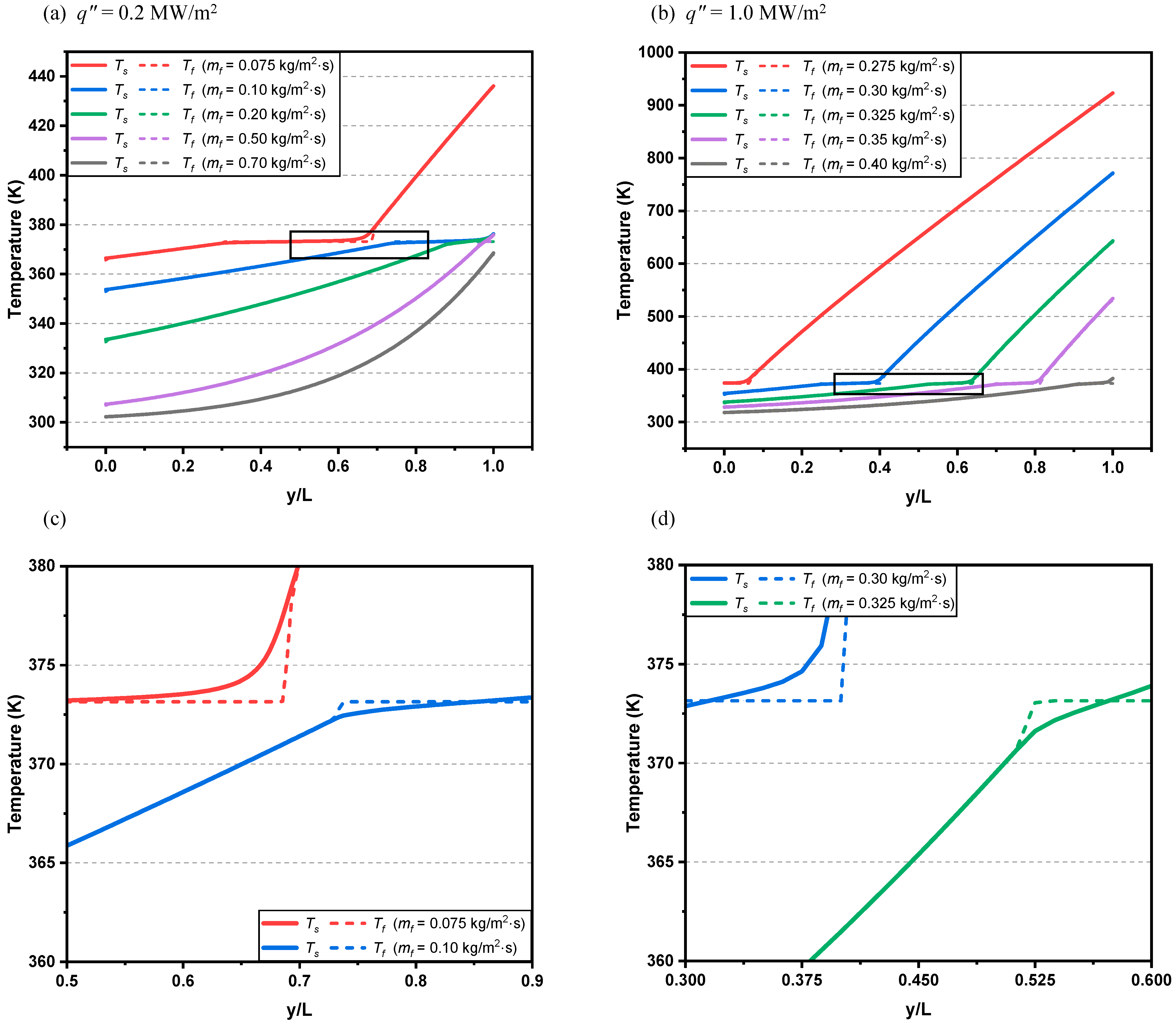
Figure 10 presents the temperature distributions for both the solid matrix and the fluid along the flow direction for various coolant mass flow rates under heat flux conditions of q″ = 0.2 MW/m2 and q″ = 1.0 MW/m2. The temperature distributions are characterized by three distinct regions, consistent with the liquid saturation analysis—a superheated vapor region near the hot surface, a two-phase region where the fluid remains at its saturation temperature, and a single-phase liquid region near the coolant inlet. A key observation is that the temperature gradient within the vapor region is much steeper than in the liquid region. This phenomenon is mainly due to the difference in thermal conductivity. The liquid phase has a much higher thermal conductivity than the vapor phase, so a steeper temperature gradient is required to transfer heat from the vapor region for the same heat flow rate. In addition, as the coolant flow rate increases, the superheated vapor region compresses. The shorter length of this vapor region, combined with its lower thermal conductivity, results in a steeper temperature gradient in this small area.
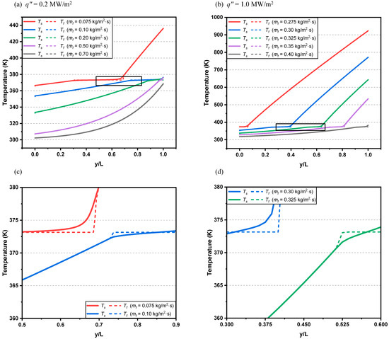
Figure 10.
Temperature distributions along flow direction at different coolant mass fluxes under (a) q″ = 0.2 MW/m2 and (b) q″ = 1.0 MW/m2. The corresponding panels (c,d) present detailed views of the local temperature profiles within the phase-change region.
A primary feature highlighted by these temperature distributions is the pronounced Local Thermal Non-Equilibrium (LTNE) phenomenon. While the solid and fluid phases are in approximate thermal equilibrium in the single-phase regions, a remarkable temperature difference between them emerges as soon as phase change begins. This is because the fluid temperature remains pinned at the saturation point due to boiling heat transfer, while the solid matrix continues to absorb the incoming heat, causing its temperature to rise. Furthermore, the influence of the coolant injection rate is evident in the liquid region’s temperature distributions. As the mass flow rate increases, advective transport becomes more dominant, resulting in a more pronounced exponential-like rise in the liquid temperature from the inlet (300 K) to the saturation point (373.15 K). This exponential profile signifies that the high-velocity coolant effectively carries its low temperature deep into the porous structures, suppressing temperature rise until it approaches the phase-change boundary. While this concentrates the cooling effect near the inlet, it also creates a sharp thermal gradient at the interface.
A comparison between a representative low heat flux case (q″ = 0.2 MW/m2, mf = 0.075 kg/m2·s) and a high heat flux case (q″ = 1.0 MW/m2, mf = 0.30 kg/m2·s) reveals the unexpected effect of the thermal load on the overall temperature distribution. In the low heat flux case, the two-phase region is observed to be significantly wider. This occurs because the lower thermal energy input is insufficient to cause immediate and complete vaporization of the coolant supplied by capillary action. Instead, the phase change happens gradually and is distributed over a larger volume within the porous structures. This large two-phase region results in a temperature distribution characterized by relatively low temperatures on the hot surface but much higher temperatures on the cold side. Such a distribution indicates that slow, distributed vaporization allows more thermal energy to bypass the phase-change zone and conduct through the solid matrix toward the inlet. Conversely, the high heat flux case can be understood through the concept of a thermal shield. In this case, the intense thermal load causes rapid local vaporization very close to the hot surface. This phase-change process acts as an effective thermal barrier, by consuming most of the incoming heat energy for its latent heat requirement, right at the surface where the heat arrives. Since the thermal energy is so effectively consumed at this front line, very little residual heat is left to penetrate deeper into the solid matrix via conduction. Therefore, even though the hot surface itself is under extreme thermal attack, the structure’s colder, downstream regions are better protected from heat penetration, resulting in a lower temperature at the coolant inlet side compared to the low heat flux case.
Finally, a notable and unusual phenomenon is observed in the magnified temperature distributions of Figure 10c,d. Near the liquid–mixture interface, the solid matrix temperature (Ts) unexpectedly drops below the surrounding fluid temperature (Tf). This temperature inversion is attributed to the reverse flow of hot vapor from the downstream region, a complex phenomenon driven by the interplay of capillary action and phase change within the pores. The theoretical basis for this vapor counterflow can be understood from the governing equations of the two-phase mixture model. From the definition of capillary pressure and mixture fluid pressure, the individual pressure gradients for liquid and vapor phases are defined as follows:
By substituting these pressure gradients into the phase momentum equations and applying Darcy’s law, the individual mass fluxes for the liquid and vapor phases can be derived, as shown in Equations (17) and (18):
Equation (18) shows that the net vapor mass flux is determined by the interaction of two competing transport mechanisms. One is a forward convection term driven by a bulk mixture flow, and the other is a reverse capillary diffusion term driven by a saturation gradient. Near the liquid–mixture interface, a sharp saturation gradient produces a large diffusion flux, overwhelming the forward convection locally, resulting in a net negative value of the vapor mass flux. This negative flux mathematically confirms the existence of vapor counterflow.
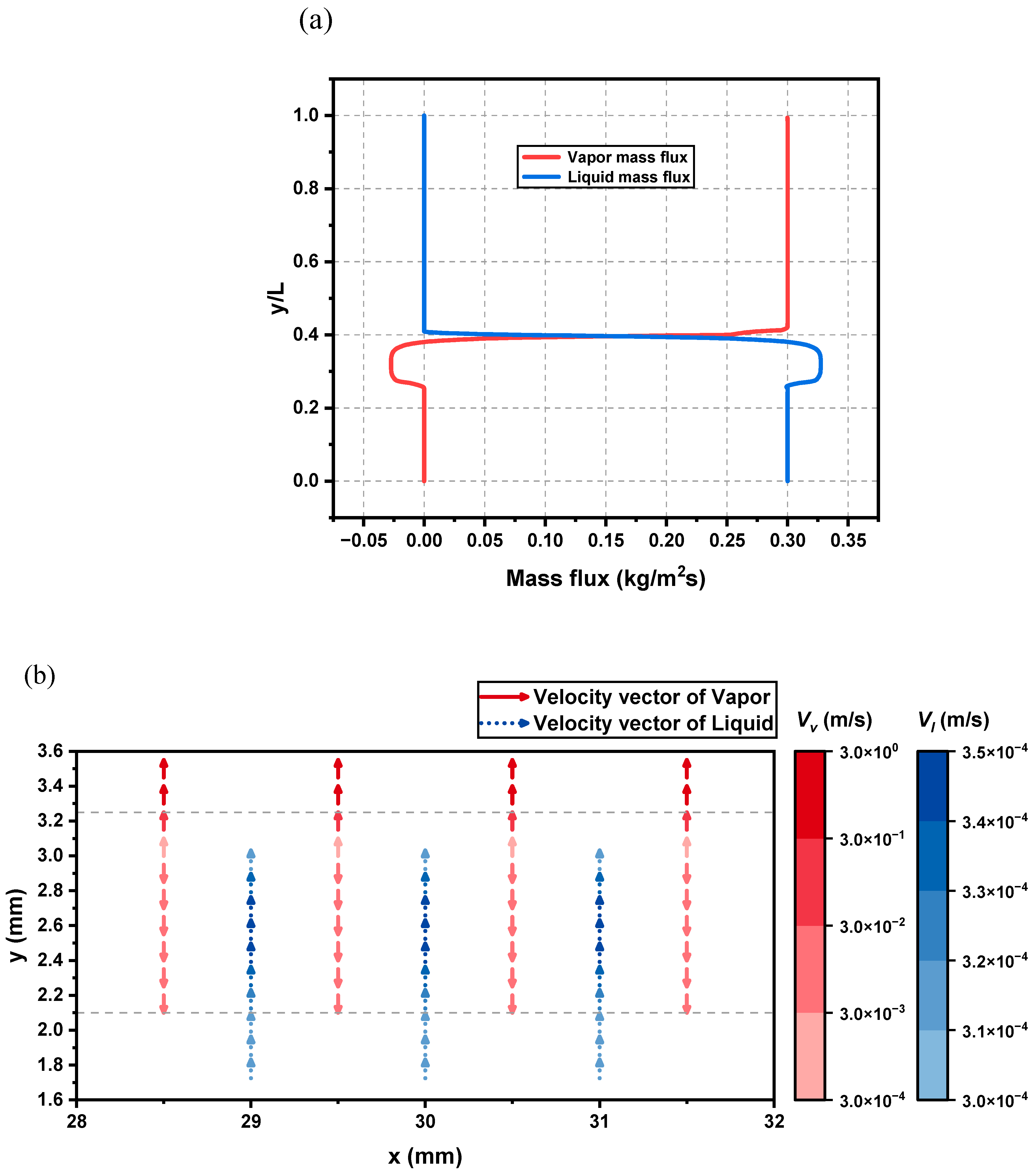
Figure 11 clearly demonstrates this counterflow by illustrating the mass flux and velocity profiles for both the liquid and vapor phases under conditions of a heat flux of 1.0 MW/m2 and coolant mass flux of 0.30 kg/m2·s. This backward movement of vapor directly impacts the liquid flow due to the principle of mass conservation. The total mass flow rate at any point must remain constant. Therefore, to compensate for the backward-flowing vapor, the forward-flowing liquid mass flux must increase in that same region, a trend that is also clearly visible in the graph. Figure 11b demonstrates this through the velocity vector field, showing the region of vapor counterflow in the downstream region. This counterflow is explained as a direct cause of the temperature inversion observed through two main physical processes. Firstly, the counterflow of vapor has high-enthalpy energy, pushing the phase-change layer at the saturation temperature downstream into the liquid-only region. This causes the fluid phase to locally heat up to saturation temperature. Secondly, condensation occurs when this hot vapor continues to flow back and mix with the supercooled liquid. This condensation releases latent heat directly into the surrounding liquid, further increasing the local fluid temperature. Meanwhile, a solid matrix in these regions is efficiently cooled by a main flow of cold liquid. As a result, a local region is created where the fluid heated by the displaced saturated line and condensation becomes paradoxically hotter than the surrounding solid matrix.

Figure 11.
(a) Individual mass flux distributions of liquid and vapor along flow direction distributions along flow direction under q″ = 1.0 MW/m2 and mf = 0.30 kg/m2·s. (b) Individual velocity vector distribution of liquid and vapor in the phase change region under q″ = 1.0 MW/m2 and mf = 0.30 kg/m2·s.
4. Conclusions
This study presents a comprehensive numerical investigation of transpiration cooling in porous structures, focusing on the complex interactions between heat transfer and phase-change phenomena associated with liquid coolant phase change. By employing a two-phase mixture model with a local thermal non-equilibrium (LTNE) approach, this study systematically analyzes the various physically coupled phenomena of temperature distribution, pressure drop, and phase change as a function of changes in key operating parameters, such as heat flux and coolant mass flow rate. The conclusions of this study are summarized as follows:
- The phase-change regime in a porous structure results from the interaction of capillary liquid replenishment and vaporization driven by heat flux. Under low heat flux conditions (q″ = 0.2 MW/m2), the mechanism whereby the capillary liquid supply rate exceeds the vaporization rate suppresses complete dry-out, even as the flow rate decreases to 0.10 kg/m2⋅s, resulting in a progressive expansion of the two-phase region. In contrast, under high heat flux conditions (q″ = 1.0 MW/m2), the evaporation rate from the intense thermal load surpasses the physical limit of the capillary supply, causing the formation of a superheated vapor layer at a higher flow rate threshold of 0.40 kg/m2⋅s and a constriction of the two-phase region.
- The pressure drop behavior in the porous medium is determined by the relative dominance between the flow rate and the fluid kinematic viscosity, which are two key factors constituting Darcy’s law. At low flow rates, increased flow suppresses evaporation, reducing high-viscosity vapor phases and decreasing the average kinematic viscosity, which paradoxically reduces total pressure drop despite higher flow rates. Beyond a transition point where single-phase liquid dominates, the kinematic viscosity becomes constant, allowing flow rate effects to dominate. Consequently, the system returns to typical Darcy flow behavior, with pressure drop increasing monotonically with flow rate.
- A temperature inversion phenomenon in which the local solid matrix temperature is lower than the ambient fluid temperature was observed at the liquid–mixture interface where phase change occurs. The direct physical cause for this is the counterflow of vapor from downstream against the primary flow direction. This vapor counterflow acts as a direct mechanism for inducing a local fluid temperature higher than the solid temperature through two main physical processes: first, when convection of high-enthalpy vapor moves the saturation boundary to the cooler liquid region downstream; second, when the vapor is mixed with the supercooled liquid and condenses, latent heat is released, further increasing the local fluid temperature. As a result, this reverse heat transfer process results in a paradoxical state in which the local fluid becomes hotter than the adjacent solid matrix, and the solid remains effectively cooled by the main flow.
Author Contributions
Conceptualization, T.Y.K.; methodology, T.Y.K.; validation, J.B. and J.S.; formal analysis, J.B. and J.S.; data curation, J.B. and J.S.; writing—original draft preparation, J.B.; writing—review and editing, T.Y.K.; supervision, T.Y.K.; funding acquisition, T.Y.K. All authors have read and agreed to the published version of the manuscript.
Funding
This research was supported by the Korea Research Institute for defense Technology planning and advancement (KRIT), grant funded by the Korean government (DAPA (Defense Acquisition Program Administration)) (No. KRIT-CT-22-030, Reusable Unmanned Space Vehicle Research Center, 2025). Also, this research was supported by the Technology Innovation Program (RS-2024-00486922, Development of a Thermoelectric Device-Based Smart Heat Dissipation Module for Semiconductor Test Modules) funded By the Ministry of Trade Industry & Energy (MOTIE, Republic of Korea).
Data Availability Statement
Data will be made available on request.
Conflicts of Interest
The authors declare no conflicts of interest.
Abbreviations
The following abbreviations and nomenclature are used in this manuscript:
| SPM | Separated Phase Model |
| TPMM | Two-Phase Mixture Model |
| LTE | Local Thermal Equilibrium |
| LTNE | Local Thermal Non-Equilibrium |
| FVM | Finite Volume Method |
| UDFs | User-Defined Functions |
| UDS | User-Defined Scalar |
| UDM | User-Defined Memory |
| Nomenclature | |
| cp | Specific heat (J/kg⋅K) |
| cs, f | Constant in Rohsenow correlation |
| dp | Average particle diameter (m) |
| h | Specific enthalpy (J/kg) |
| hfg | Latent heat of vaporization (J/kg) |
| K | Absolute permeability (m2) |
| k | Thermal conductivity (W/m⋅K) |
| krl, krv | Relative permeabilities of liquid and vapor |
| L | Thickness of porous plate (m) |
| mf | Coolant mass flux (kg/m2⋅s) |
| P | Pressure (Pa) |
| Pr | Prandtl number |
| q″ | Heat flux (W/m2) |
| Re | Reynolds number |
| s | Liquid saturation |
| T | Temperature (K) |
| Velocity vector (m/s) | |
| Greek symbols | |
| ε | Porosity |
| ν | Kinematic viscosity (m2/s) |
| μ | Dynamic viscosity (kg/m·s) |
| ρ | Density (kg/m3) |
| λ | Relative mobility |
| σ | Interfacial tension (N/m) |
| γh | Advection coefficient |
| Γ | Effective diffusion coefficient (kg/m·s) |
| Subscripts | |
| f | Fluid |
| s | Solid |
| l | Liquid |
| v | Vapor |
| sat | Saturated |
| c | Capillary |
| eff | Effective |
| sf | Solid–fluid |
| boil | Boiling |
Appendix A
Appendix A.1. Constitutive Relationships in LTNE–TPMM
Table A1.
Constitutive relationships in LTNE–TPMM [9,17,20].
References
- Cerminara, A.; Deiterding, R.; Sandham, N.D. Transpiration cooling using porous material for hypersonic applications. In Convective Heat Transfer in Porous Media; CRC Press: Boca Raton, FL, USA, 2019; pp. 263–286. [Google Scholar]
- Mi, Q.; Yi, S.; Gang, D.; Lu, X.; Liu, X. Research progress of transpiration cooling for aircraft thermal protection. Appl. Therm. Eng. 2024, 236, 121360. [Google Scholar] [CrossRef]
- Jackson, T.A.; Eklund, D.R.; Fink, A.J. High speed propulsion: Performance advantage of advanced material. J. Mater. Sci. 2004, 39, 5905–5913. [Google Scholar] [CrossRef]
- Laganelli, A. A comparison between film cooling and transpiration cooling systems in high speed flow. In Proceedings of the 8th Aerospace Sciences Metting, West Germany, 19–21 January 1970. [Google Scholar] [CrossRef]
- Landis, J.; Bowman, W. Numerical study of a transpiration cooled rocket nozzle. In Proceedings of the 32nd Joint Propulsion Conference and Exhibit, Lake Buena Vista, FL, USA, 1–3 July 1996. [Google Scholar] [CrossRef]
- Herbertz, A.; Ortelt, M.; Müller, I.; Hald, H. Transpiration cooled ceramic thrust chamber applicability for high-thrust rocket engines. In Proceedings of the 48th AIAA/ASME/SAE/ASEE Joint Propulsion Conference & Exhibit, Atlanta, GA, USA, 30 July–1 August 2012; p. 3990. [Google Scholar] [CrossRef]
- Arai, M.; Suidzu, T. Porous ceramic coating for transpiration cooling of gas turbine blade. J. Therm. Spray Technol. 2013, 22, 690–698. [Google Scholar] [CrossRef]
- Polezhaev, J. The transpiration cooling for blades of high temperatures gas turbine. Energy Convers. Manag. 1997, 38, 1123–1133. [Google Scholar] [CrossRef]
- Su, H.; Wang, J.; He, F.; Chen, L.; Ai, B. Numerical investigation on transpiration cooling with coolant phase change under hypersonic conditions. Int. J. Heat Mass Transf. 2019, 129, 480–490. [Google Scholar] [CrossRef]
- Zhao, L.; Wang, J.; Ma, J.; Lin, J.; Peng, J.; Qu, D.; Chen, L. An experimental investigation on transpiration cooling under supersonic condition using a nose cone model. Int. J. Therm. Sci. 2014, 84, 207–213. [Google Scholar] [CrossRef]
- van Foreest, A.; Sippel, M.; Gülhan, A.; Esser, B.; Ambrosius, B.A.C.; Sudmeijer, K. Transpiration cooling using liquid water. J. Thermophys. Heat Transf. 2009, 23, 693–702. [Google Scholar] [CrossRef]
- Huang, G.; Zhu, Y.; Liao, Z.; Ouyang, X.L.; Jiang, P.X. Experimental investigation of transpiration cooling with phase change for sintered porous plates. Int. J. Heat Mass Transf. 2017, 114, 1201–1213. [Google Scholar] [CrossRef]
- Luan, Y.; He, F.; Wang, J.; Wu, Y.; Zhu, G. An experimental investigation on instability of transpiration cooling with phase change. Int. J. Therm. Sci. 2020, 156, 106498. [Google Scholar] [CrossRef]
- Xin, C.; Rao, Z.; You, X.; Song, Z.; Han, D. Numerical investigation of vapor–liquid heat and mass transfer in porous media. Energy Convers. Manag. 2014, 78, 1–7. [Google Scholar] [CrossRef]
- He, F.; Wang, J.; Xu, L.; Wang, X. Modeling and simulation of transpiration cooling with phase change. Appl. Therm. Eng. 2013, 58, 173–180. [Google Scholar] [CrossRef]
- He, F.; Wang, J. Numerical investigation on critical heat flux and coolant volume required for transpiration cooling with phase change. Energy Convers. Manag. 2014, 80, 591–597. [Google Scholar] [CrossRef]
- Wang, C.-Y.; Beckermann, C. A two-phase mixture model of liquid-gas flow and heat transfer in capillary porous media—I. Formulation. Int. J. Heat Mass Transf. 1993, 36, 2747–2758. [Google Scholar] [CrossRef]
- Wang, C.Y. A fixed-grid numerical algorithm for two-phase flow and heat transfer in porous media. Numer. Heat Transf. 1997, 32, 85–105. [Google Scholar] [CrossRef]
- Hu, H.; Jiang, P.; Ouyang, X.; Zhao, C.; Xu, R. A modified energy equation model for flow boiling in porous media and its application to transpiration cooling at low pressures with transient effect. Int. J. Heat Mass Transf. 2020, 158, 119745. [Google Scholar] [CrossRef]
- Shi, J.X.; Wang, J.H. A numerical investigation of transpiration cooling with liquid coolant phase change. Transp. Porous Media 2011, 87, 703–716. [Google Scholar] [CrossRef]
- Alomar, O.R.; Mendes, M.A.; Trimis, D.; Ray, S. Numerical simulation of complete liquid–vapour phase change process inside porous media: A comparison between local thermal equilibrium and non-equilibrium models. Int. J. Therm. Sci. 2017, 112, 222–241. [Google Scholar] [CrossRef]
- Marafie, A.; Vafai, K. Analysis of non-Darcian effects on temperature differentials in porous media. Int. J. Heat Mass Transf. 2001, 44, 4401–4411. [Google Scholar] [CrossRef]
- Jin, K.; Zhao, J.; Yao, G.; Wen, D. A modified local thermal non-equilibrium model of transient phase-change transpiration cooling for hypersonic thermal protection. Adv. Aerodyn. 2024, 6, 12. [Google Scholar] [CrossRef]
- Liu, T.; Su, H.; Chen, Z.; He, F.; Wang, J. Numerical investigation on the transient transport and heat transfer characteristics of transpiration cooling with liquid phase change during coolant adjustment. Appl. Therm. Eng. 2022, 209, 118277. [Google Scholar] [CrossRef]
- Shin, J.; Bae, J.; Kim, S.J.; Kim, T.Y. Flow regimes and flow instability of transpiration cooling. Int. J. Heat Mass Transf. 2025; in press. [Google Scholar] [CrossRef]
- Chen, Y.; Du, S.; Li, D.; Gao, Y.; He, Y.L. Numerical investigation of transient phase-change transpiration cooling based on variable properties of coolant. Appl. Therm. Eng. 2021, 184, 116204. [Google Scholar] [CrossRef]
- Zhang, T.; Tong, T.; Chang, J.Y.; Peles, Y.; Prasher, R.; Jensen, M.K.; Wen, J.T.; Phelan, P. Ledinegg instability in microchannels. Int. J. Heat Mass Transf. 2009, 52, 5661–5674. [Google Scholar] [CrossRef]

Disclaimer/Publisher’s Note: The statements, opinions and data contained in all publications are solely those of the individual author(s) and contributor(s) and not of MDPI and/or the editor(s). MDPI and/or the editor(s) disclaim responsibility for any injury to people or property resulting from any ideas, methods, instructions or products referred to in the content. |
© 2025 by the authors. Licensee MDPI, Basel, Switzerland. This article is an open access article distributed under the terms and conditions of the Creative Commons Attribution (CC BY) license (https://creativecommons.org/licenses/by/4.0/).