Article

Modeling the Higher Heating Value of Spanish Biomass via Neural Networks and Analytical Equations

by
Anbarasan Jayapal
1,†,
Fernando Ordonez Morales
1,†,
Muhammad Ishtiaq
1,
Se Yun Kim
1,* and
Nagireddy Gari Subba Reddy
2,*
1
Department of Materials Engineering and Convergence Technology, Gyeongsang National University, Jinju 52828, Republic of Korea
2
School of Materials Science and Engineering, Engineering Research Institute, Gyeongsang National University, Jinju 52828, Republic of Korea
*
Authors to whom correspondence should be addressed.
These authors contributed equally to this work.
Energies 2025, 18(15), 4067; https://doi.org/10.3390/en18154067 (registering DOI)
Submission received: 30 June 2025 / Revised: 21 July 2025 / Accepted: 28 July 2025 / Published: 31 July 2025

Abstract

Accurate estimation of biomass higher heating value (HHV) is crucial for designing efficient bioenergy systems. In this study, we developed a Backpropagation artificial neural network (ANN) that predicts HHV from routine proximate/ultimate composition data. The network (9-6-6-1 architecture, trained for 15,000 epochs with learning rate 0.3 and momentum 0.4) was calibrated on 99 diverse Spanish biomass samples (inputs: moisture, ash, volatile matter, fixed carbon, C, H, O, N, S). The optimized ANN achieved strong predictive accuracy (validation R2 ≈ 0.81; mean squared error ≈ 1.33 MJ/kg; MAE ≈ 0.77 MJ/kg), representing a substantial improvement over 54 analytical models despite the known complexity and variability of biomass composition. Importantly, in direct comparisons it significantly outperformed 54 published analytical HHV correlations—the ANN achieved substantially higher R2 and lower prediction error than any fixed-form formula in the literature. A sensitivity analysis confirmed chemically intuitive trends (higher C/H/FC increase HHV; higher moisture/ash/O reduce it), indicating the model learned meaningful fuel-property relationships. The ANN thus provided a computationally efficient and robust tool for rapid, accurate HHV estimation from compositional data. Future work will expand the dataset, incorporate thermal pretreatment effects, and integrate the model into a user-friendly decision-support platform for bioenergy applications.

1. Introduction

Renewable energy sources are widely sought as alternatives to fossil fuels, with biomass emerging as a particularly promising choice due to their abundance and potential for carbon neutrality [1]. Biomass includes diverse organic elements, such as agricultural residues, forestry outputs, specific energy crops, and organic waste, which can be trans-formed into power or biofuels [2]. A critical metric for biomass fuels is the higher heating value (HHV), which measures the total energy released upon complete combustion [3]. Fuels with elevated HHVs produce greater energy; yet the direct measurement of HHV by bomb calorimetry is both time-intensive and expensive [4]. Consequently, many predictive models have been proposed to estimate the HHV from more easily measured fuel properties.
Numerous analytical equation correlations have been formulated to predict the HHV from biomass composition obtained via ultimate (elemental) or proximate (bulk property) analysis [5,6]. These analytical equations (often linear or polynomial) allow for the estimation of HHVs from factors, such as carbon content or moisture and ash levels, avoiding the need for experimental calorimetry. However, such basic models often lack accuracy and generality for a wide range of biomass feedstocks, as they fail to strongly represent nonlinear relationships between composition and energy content [7]. This constraint has led to the adoption of data-driven machine learning techniques, particularly artificial neural networks (ANNs), to forecast HHVs with greater reliability [8]. ANNs excel at representing complex, nonlinear interactions by learning directly from input without assuming a predetermined functional structure [9]. Research indicates that ANN-based HHV predictions have markedly enhanced accuracy relative to conventional correlations [10]. An ANN model trained on 532 distinct biomass samples produced significantly more precise HHV estimations than any linear equation [11], while another model attained experimental-level accuracy for bamboo biomass, exhibiting robust generalization across samples [10].
Most Prior ANN models have utilized either proximate or ultimate analysis data as inputs, not both. This is despite the progress that has been made. Proximate analysis provides information regarding the fundamental properties of fuel qualities, like moisture, ash, volatile matter, and fixed carbon. Ultimate analysis tells you about the elemental composition, like carbon, hydrogen, oxygen, nitrogen, and sulfur. Both types of analysis give you useful information on the quality of biomass. Combining these data could make predictions more accurate by giving a fuller picture of the fuel. Recent research backs up this idea. Güleç et al. used an ANN that combined both proximate and ultimate variables to make better HHV predictions across a range of feedstocks [12]. Aghel et al. [13] used a dynamic Elman network on a dataset of over 500 samples and showed that it worked well.
We developed a reliable ANN model to predict the HHV of diverse Spanish biomass samples from their combined proximate and ultimate analysis data. The novelty of this study lies both in its comprehensive scope and specific focus. Unlike the prior ANN-based HHV studies by Güleç et al. [12] and Aghel et al. [13] (which also utilized proximate and ultimate inputs), this work provides several distinct contributions: it benchmark’s the ANN’s performance against 54 analytical models—a far broader comparison than in previous studies—to firmly establish its accuracy gains. We further make this model into a practical tool by developing a GUI, facilitating the real-world application of our results. Another unique aspect is the focus on Spanish biomass samples, offering region-specific insights that complement the broader datasets used in [12,13]. Additionally, this work enhances interpretability through an Index of Relative Importance (IRI) analysis to quantify each input’s influence on the HHV, an analysis not reported in earlier works, by integrating both proximate and elemental data. This approach capitalizes on a more complete set of fuel characteristics, yielding more accurate predictions than models relying on a single type of analysis.

2. Materials and Methods

2.1. Dataset and Preprocessing

The dataset comprises 99 distinct biomass samples, which include commercial fuels, industrial waste (leaves and branches), energy crops, and cereals. The complete set of proximate and ultimate analysis values used in this study was adopted from two companion papers by García et al. [14,15] which provide a comprehensive characterization of Spanish biomass samples using standardized experimental protocols. As described in their methodology, the proximate analysis followed ASTM guidelines, with biomass samples first air-dried and then ground to a particle size of 1 mm prior to measurement. Ultimate analysis was performed through elemental analysis using standard ASTM-based procedures. For the determination of higher heating values (HHVs), a bomb calorimeter (IKA Werke C 5000 control) was employed in accordance with the ASTM E711 method [16,17]. The use of consistent, well-established laboratory protocols across all samples ensures high data reliability and uniformity, making the dataset well-suited for developing and validating machine learning models for HHV prediction.
Each sample is characterized by nine input features: moisture content (M), ash content (A), volatile matter (VM), fixed carbon (FC), and the elemental contents of carbon (C), hydrogen (H), nitrogen (N), sulfur (S), and oxygen (O). These parameters were obtained from standard proximate (M, A, VM, FC) and ultimate (C, H, N, S, O) analyses, and are known to strongly influence biomass fuel properties such as the HHV. Table 1 summarized the descriptive statistics (minimum, mean, maximum, and standard deviation) for each of the nine inputs. The original dataset compiled by García et al. [14,15] included 100 samples, but was reduced to 99 samples after removing one outlier.
The removed outlier corresponded to vegetal coal, which exhibited an extremely high HHV value well above the typical range observed for lignocellulosic biomass (i.e., ~15–20 MJ/kg). Although vegetal coal can have elevated carbon content, the recorded value was physically implausible and inconsistent with the rest of the dataset. To avoid distortion of model training and to maintain dataset homogeneity, this sample was excluded. The complete dataset is provided in Table S1. The target output for the ANN was the biomass HHV on a dry basis (MJ/kg). Prior to training, all inputs and the HHV output were rescaled by min–max normalization to the [0.1 to 0.9] range. This feature scaling is a standard preprocessing step in neural network modeling as it prevents large differences in value magnitudes and facilitates numerical stability and consistent training performance. Consistent with standard practice, the 99 samples were split into 75 for training and 24 for testing (approximately a 75%/25% partition). Figure 1 illustrates the comprehensive modeling procedure, including data preparation, training/testing partition, neural network architecture, and evaluation metrics. To accelerate the convergence and to improve model stability, data normalization was performed using Equation (1) [18].
X n = X X m i n × 0.8 ( X m a x X m i n ) + 0.1
where Xn denotes the normalized value of X, while Xmax and Xmin represent the maximum and minimum values of X, respectively, across the whole dataset. The data normalization ensured that all input variables contributed equally to the training process, preventing features with larger numerical ranges from dominating the learning. Upon identifying the optimal network, all changed data were reverted to their original values using Equation (2) [18].
X = X n 0.1 × ( X m a x X m i n ) 8 + X m i n
The reversion of the normalized data allowed us to perform a meaningful interpretation and comparison with the previously published data. Table 2 summarizes the final hyperparameters of the ANN model.

2.2. ANN Model Architecture

A backpropagation-based artificial neural network (BP-ANN) was employed to predict the HHV from the biomass composition inputs. ANN models are effective in modeling complex, nonlinear relationships in biomass fuel datasets. The network had an input layer with 9 neurons (M, A, VM, FC, N, C, S, H, O), Three network configurations were evaluated: (i) a single hidden layer (9-6-1), (ii) two hidden layers (9-6-6-1), and (iii) three hidden layers (9-6-6-6-1) up to 25 neurons each, and an output layer with a single output neuron responsible for HHV prediction. To evaluate the model, the dataset of 99 biomass samples was randomly split into 75 training and 24 testing samples (~75/25 split). This partitioning preserved the overall distribution of the HHV and compositional variables, allowing for meaningful training and external testing. While k-fold cross-validation is commonly used for small datasets, in this study, we prioritized a fixed test set to provide a clear and consistent evaluation of generalization performance. Future work will incorporate k-fold or repeated cross-validation techniques as part of a broader investigation into model robustness and uncertainty quantification. The logistic sigmoid function was used by all the neurons. This activation function is well-suited for continuous regression problems with normalized objectives, and is one of the most common transfer functions used in multilayer neural networks. A recent in-depth study [19] on modeling biomass HHV indicated that ANN models with non-linear sigmoidal activation functions are better at making predictions than those with linear activation functions. Analytical tuning was applied to choose the number of hidden layers and neurons such that the model would be both sufficiently complex and high performing. The hyperparameters were optimized using manual tuning based on iterative performance evaluation, changing the size of the network until the prediction error is minimized. Specifically, the network was tested with 1, 2, and 3 hidden layers, varying each hidden layer from 6 up to 25 neurons; R2 values improved as neuron count increased, reaching a plateau near 25, so the 25-neuron configuration was selected as it provided the best trade-off between accuracy and avoiding overfitting. The three-layer architecture with 25 neurons per hidden layer provided adequate learning capacity to model the underlying relationships without overfitting, given the size of the dataset.

2.3. Training Procedure

Backpropagation was used to train the neural network, with a learning rate of 0.3 and a momentum coefficient of 0.4. The learning rate and momentum were empirically tested across a wide range (0.1–0.9); the values of 0.3 (learning rate) and 0.4 (momentum) consistently produced high R2 values across model configurations, so these initial values were selected based on the trial results before further fine-tuning. The momentum term accelerates convergence and stabilizes weight updates, which helps avoid entrapment in shallow local minima. The network weights were initialized randomly, followed by training using gradient descent to minimize the mean squared error (MSE) between the predicted and the actual HHV values. The loss function was the MSE. The training lasted for 15,000 epochs, consistent with durations reported in prior ANN-based studies. By that time, the training error had leveled off. After the last model was trained (with fixed weights), it was tested on a separate test set using standard performance metrics (prediction error and goodness-of-fit) to examine its generalization performance on previously unseen data. All models were implemented in Java (1.4) sing standard machine learning packages to ensure reproducibility and computational consistency.

2.4. Scatter Matrix Plots

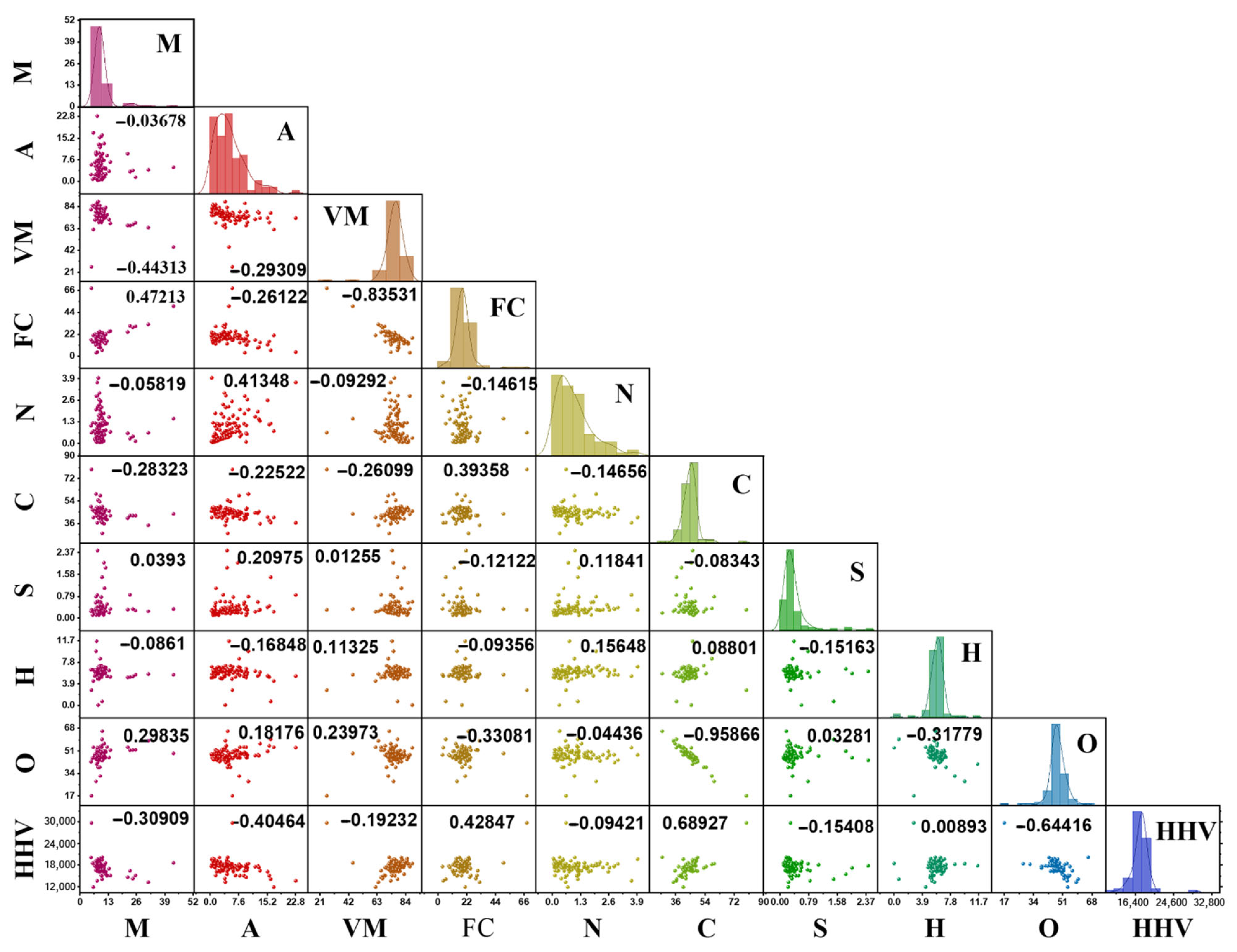
Figure 2 presents a pairwise scatterplot matrix (pair plot) with Pearson’s r value of the nine input features and the target HHV for the 99 biomass samples. The input variables are moisture (M), ash (A), volatile matter (VM), fixed carbon (FC), nitrogen (N), carbon (C), sulfur (S), hydrogen (H), and oxygen (O), while the output is the higher heating value (HHV). In this matrix, each diagonal cell demonstrates the univariate distribution (histogram) of that variable, and each off-diagonal cell demonstrates the scatter plot of one versus another. This layout enables visualization of the distribution of each variable and the pairwise relationships among variables. For example, the diagonal histograms illustrate the spread and skewness of each feature’s distribution (e.g., M exhibits right-skewness, indicating that most samples have relatively low moisture, while FC or HHV distributions appear approximately normal), while the off-diagonal scatterplots show the relationships among features. Samples with a higher FC or higher total carbon tend to lie toward a higher HHV, resulting in a positive correlation in the corresponding scatter plots. Conversely, a negative correlation is observed for samples with higher moisture or higher ash: fuels with more M or A content generally have lower HHVs (a downward-sloping pattern) [14]. Hydrogen content also demonstrates a positive association with HHVs (hydrogen-rich fuels are associated with higher combustion energy release), whereas oxygen (and to a lesser extent sulfur) is inversely related to the HHV (more oxygen/sulfur means somewhat lower energy content).
Volatile matter and nitrogen display relatively weak or negligible trends with the HHV in these plots, which is consistent with analyses that find minimal impact of N (and only a slight effect of VM) on heating value. Thus, the figure illustrates that FC and C are positively correlated with the HHV, while M and A are negatively correlated, with other elements (H, O, S, N, VM) exhibiting either weak or inconsistent associations with the HHV.

2.5. Correlation Heatmap

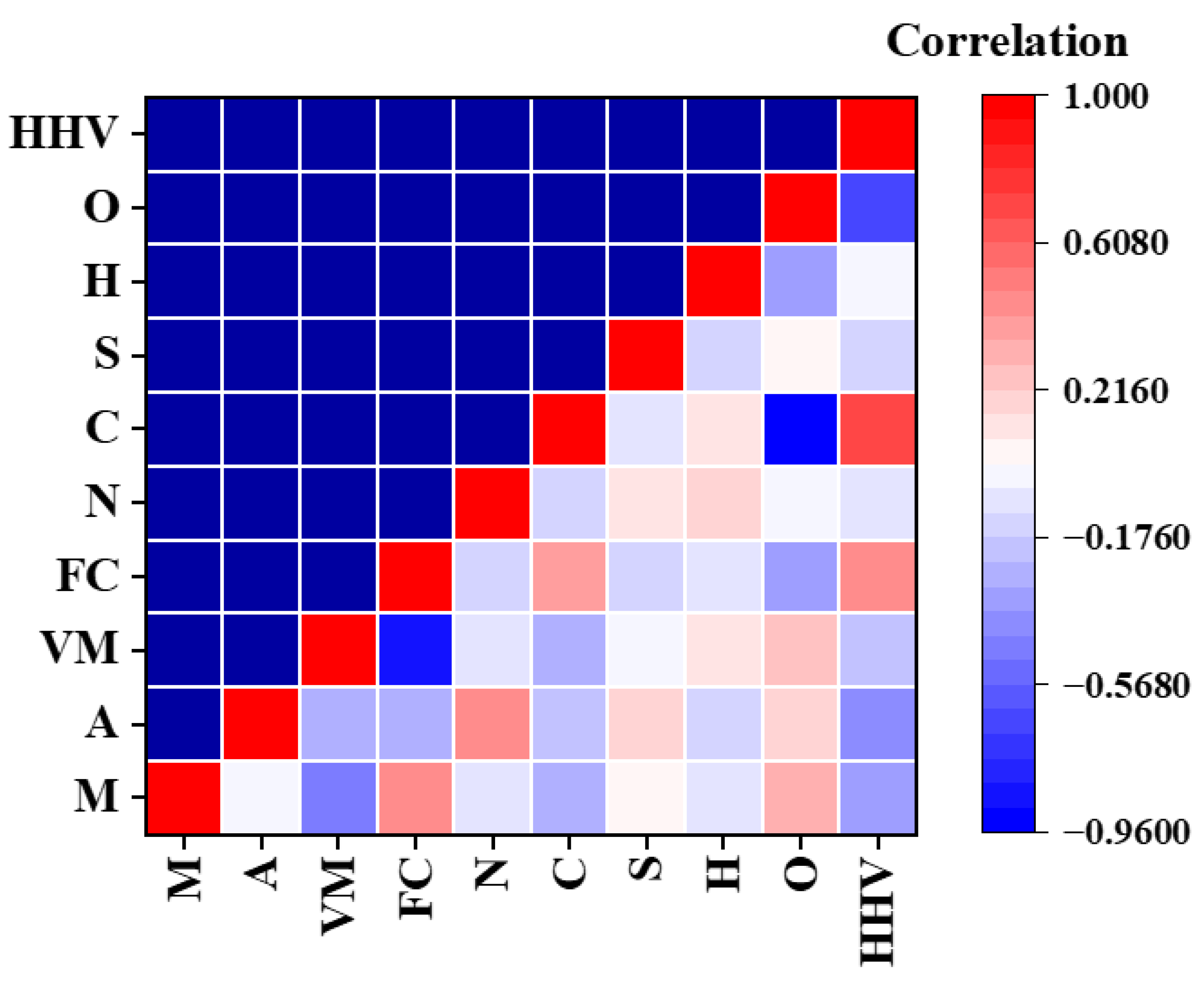
Figure 3 displays the Pearson correlation matrix for the nine input variables and the target HHV (higher heating value) over 99 biomass samples. Each cell represents the Pearson correlation coefficient between two variables, where color intensity and hue represent the strength and direction of the correlation (deep blue = strong negative, deep red = strong positive). Notably, FC and C exhibit the strongest positive correlations with HHV (bright red cells), reflecting that biomass with higher carbon content is associated with elevated HHV values. Conversely, M and A) show pronounced negative correlations with HHV (deep blue), in line with the understanding that the presence of moisture or inert ash reduces the effective heating value.
The matrix also reveals inter-variable relationships: for example, FC and VM are strongly inversely related (high FC implies low VM), and C and O contents are inversely correlated (biomass samples with a higher carbon content generally exhibit a lower oxygen content). The observed color gradients in Figure 3 visually summarize how the key compositional variables co-vary, and how those trends align with their impact on the HHV.

3. Results and Discussion

3.1. Transformation of the ANN Model Synaptic Weights

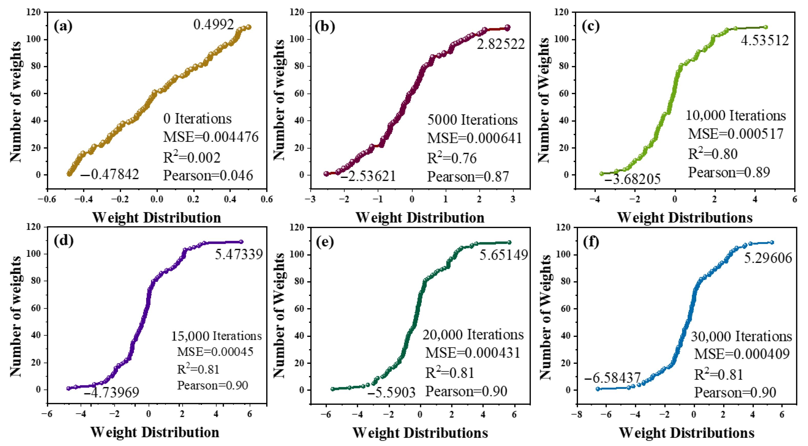
Figure 4 demonstrates how the weight distributions and performance indicators evolved as the ANN model during the training process. Figure 4a demonstrates that the connection weights are chosen at random from a symmetric distribution that is centered around zero. The initial weight histogram is very close to zero because of this, and the model has not yet learned a meaningful mapping from inputs to output, as is expected for an untrained network to have a low coefficient of determination (R2) and Pearson’s correlation coefficient (R), as well as a high mean squared error (MSE).
During training, the weights progressively diverge as the network learns (see Figure 4b,c at 5000 and 10,000 iterations). This is because updates based on gradients increase the magnitudes of many weights in both positive and negative directions. The weight histograms exhibit bigger ranges at these points: roughly ±2–3 at 5000 iterations and ±4–5 at 10,000 iterations. At the same time, the predictive performance improves substantially: R2 rises from virtually zero to approximately 0.80, and Pearson’s r goes up to around 0.89, suggesting that the network is learning statistically meaningful associations within the data. The histograms begin to exhibit a heavy-tailed distribution, with a few weights getting quite big while most stay moderate. Such behavior is typical for trained neural networks [20].
With 15,000 iterations (Figure 4d), the model approaches convergence. The weight range is roughly ±5 to 6, and the cumulative weight distribution produces a smooth, S-shaped curve. This means that the analytical distribution is stable. At this stage, the performance measures level off. The R2 stays around 0.81, while Pearson’s r stays close to 0.90. This suggests that extra training yields diminishing returns, which is what the research says about the weight distribution stabilizing even when individual weights keep changing [21].
After 15,000 iterations, training more (Figure 4e,f, at 20,000 and 30,000 iterations) does not alter much. The weight histograms and performance measures appear almost the same as they did after 15,000 iterations. The weight range is between 5 and 6, with only minor fluctuations. This signifies that the model has reached convergence, and that training it more will not make the predictions significantly better. It is usual to employ early halting when the validation performance levels off to save time on unneeded computing.
Figure 4 demonstrates how the network progresses from being untrained (with weights near to zero and poor predictive performance) to being well-optimized after around 15,000 iterations. The weight distribution transitions from narrow and centered to broad and heavy-tailed, reflecting the network’s increasing capacity to capture complex patterns. The performance measurements and weight distributions have settled down at this stage, so extra training does not help very much. Thus, 15,000 iterations are identified as a practical stopping point.

3.2. Neural Network Architecture and Hyperparameter Tuning Results

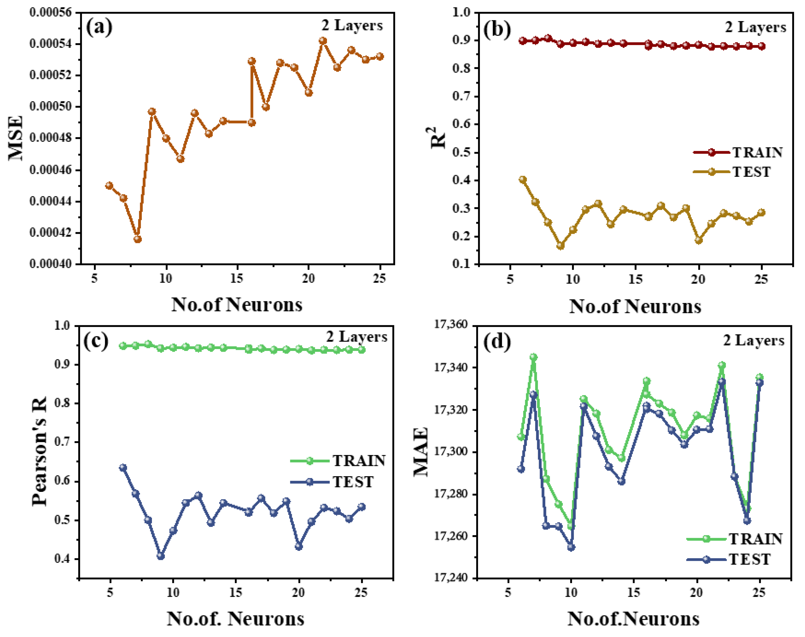
The comparative training results for the one-layer (9-6-1), two-layer (9-6-6-1), and three-layer (9-6-6-6-1) network architectures are summarized in Figure 5, Figures S1 and S2. Figure 5a–d plot the mean squared error (MSE), coefficient of determination (R2), Pearson correlation, and mean absolute error (MAE) versus epochs for all three models. Across all these metrics, the two-layer (9-6-6-1) architecture consistently outperforms or exhibits superior performance. Figure 5a demonstrates that the two-layer MSE decreases to approximately zero (on the order of 10−4) by the end of training, whereas the one-layer network converges to an MSE on the order of 10−3, and the three-layer network’s MSE increases up to ~0.08 due to large oscillations. This trend is confirmed by the Supplementary Figures: Figure S2a (one-layer vs. two-layer) demonstrates the two-layer error settling essentially at 0.000, while Figure S1a (two-layer vs. three-layer) demonstrates the three-layer MSE fluctuating up to ~0.08. Similarly, the two-layer model achieves the lowest MAE (~0.02) compared to roughly 0.07 for the one-layer and ~0.12 for the three-layer (Figure 5d, Figures S1d and S2d).
In terms of correlation metrics, the two-layer network again outperforms. As shown in Figure 5b,c, the 9-6-6-1 model attains a nearly perfect fit with R2 approaching 0.99 and Pearson correlation ≈0.99. By contrast, the one-layer network reaches R2 ≈ 0.95 and Pearson ≈0.97, and the three-layer network stalls at R2 ≈ 0.80 with Pearson ≈0.86. Figures S1b,c and S2b,c confirm these trends: the two-layer curves remain high and flat, indicating a consistently strong fit, whereas the three-layer model’s R2 and Pearson curves are much lower and noisier. The 9-6-6-1 design has the greatest R2 and Pearson values (usually within 0.01 of unity) and the lowest error metrics, indicating it is more accurate and consistent at making predictions.
The stability of the two-layer network training is also notable. In all plots (Figure 5, Figures S1 and S2), the two-layer curves converge smoothly without large fluctuations, whereas the three-layer curves exhibit pronounced oscillations (especially in MSE and MAE) that suggest unstable learning. The one-layer network is stable, but it converges to a greater error, indicating insufficient model capacity. The one-layer model does not read the data well enough, resulting in greater residual error. The three-layer model may be overfitting the data or is unstable during training, resulting in erratic errors and high variability in error metrics and lower correlation scores. The two-layer 9-6-6-1 network achieves an optimal trade-off between model complexity and training stability: it has enough complexity to capture the underlying patterns yet remains trainable, leading to consistently minimal error and maximal correlation.
The quantitative comparison of Figure 5a–d, Figures S1a–d and S2a–d clearly indicates that the two-layer architecture (9-6-6-1) is superior. It achieves the lowest MSE (≈10−4) and MAE (≈0.02), and the highest R2 (≈0.99) and Pearson (≈0.99) among all tested models. Its training behavior is the most stable, indicating robust generalization performance. By contrast, the one-layer network (9-6-1) underfits (higher errors, slightly lower R2/Pearson) and the three-layer network (9-6-6-6-1) overfits or becomes unstable (large error spikes, poorer correlation). This study adopts the 9-6-6-1 ANN as the optimal architecture for further tuning of momentum and learning rate in subsequent sections.

3.3. Momentum Rate (α) Tuning

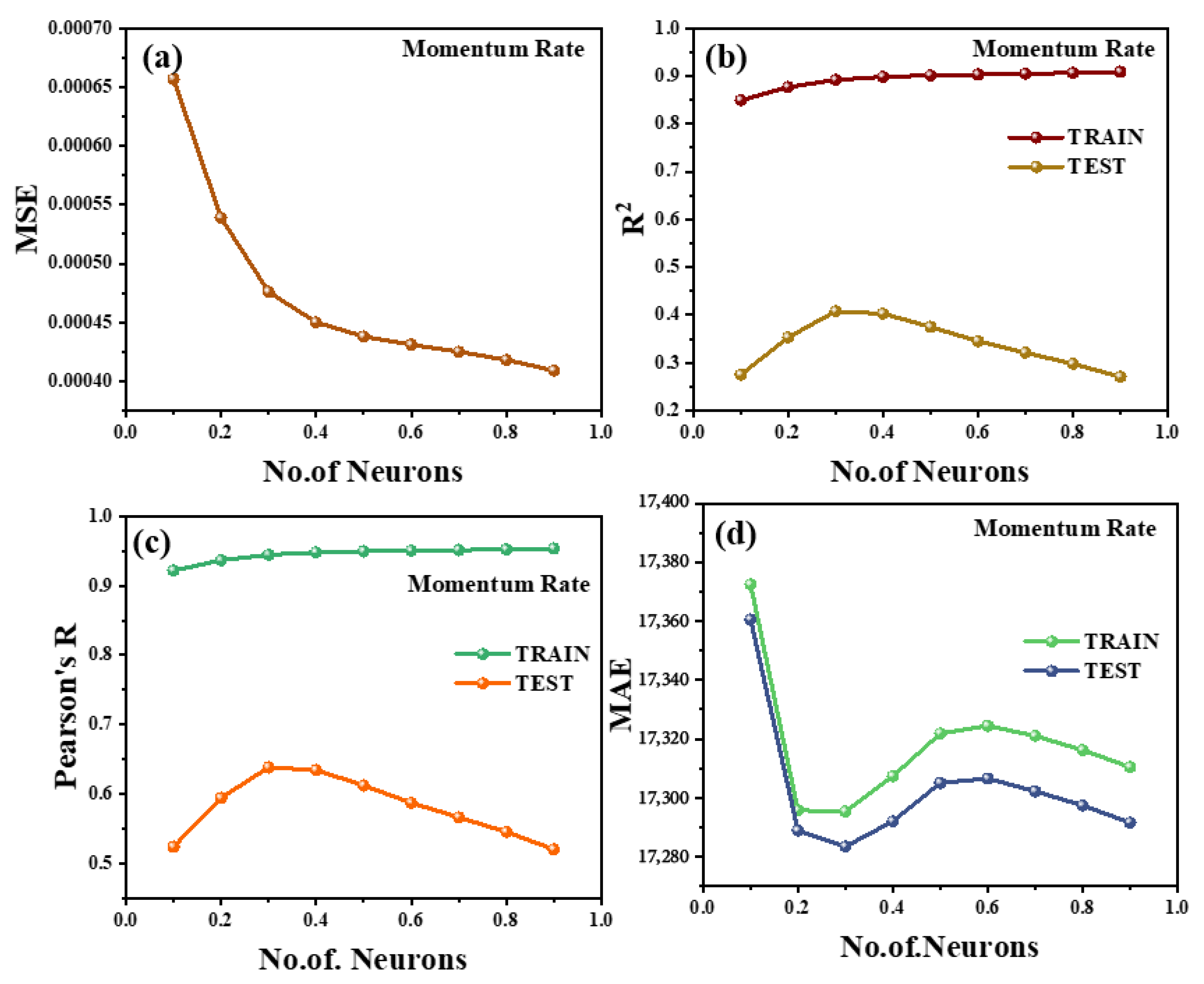
Figure 6a–d plot the 9-6-6-1 network’s MSE, R2, Pearson, and MAE as a function of hidden-layer size for different momentum values. Among the tested configurations, a momentum value of 0.4 yields the lowest prediction errors: at six neurons the MSE is about 0.98 (≈15–20% below the next best momentum = 0.3, and significantly lower than ≈1.20 for momentum = 0.5). The MAE (Figure 6d) similarly reaches a minimum value of approximately 0.26 for momentum = 0.4 (vs. ≈0.30–0.33 for the other curves). In parallel, R2 and Pearson (Figure 6b,c) achieve maximum values of approximately 0.86 and 0.93, respectively, for momentum = 0.4 at six neurons, exceeding all other settings (e.g., R2 ≈ 0.75–0.80, r ≈ 0.88–0.90 for lower momentum). R2 ≈ 0.86 implies that about 86% of the variance is explained by the model, and r ≈ 0.93 indicates a very strong linear fit. Collectively, the momentum = 0.4 configuration has the best accuracy (lowest error, highest fit), consistent with the known effect that momentum speeds convergence and help avoid local minimum. By contrast, momentum = 0.5 yields nearly flat, high-error curves (Figure 6a,d)—the network fails to converge properly, suggesting unstable oscillations during training—and very low momentum (e.g., 0.1) converges at a slower rate (higher residual error).
As neurons increase beyond the optimum (~6), this behavior reflects the expected bias–variance tradeoff. All curves exhibit high error values initially for very small networks (2–4 neurons), indicating underfitting. For momentum = 0.4 the loss function decreases rapidly up to about 6–8 neurons, then plateaus or increases marginally, R2 and Pearson begin to decline past ~6–8 neurons (Figure 6b,c), and MSE/MAE plateau (Figure 6a,d), suggesting that increasing the number of neurons beyond the optimal range does not improve model performance and may introduce overfitting (and possible overfitting to data noise). Lower momentum curves (0.1–0.3) improve more gradually with neuron count, reflecting slower convergence, and never reach the same performance peak. Overall, Figure 6 demonstrates that moderate momentum (0.4) achieves rapid convergence with minimal error, whereas excessive momentum causes divergence/oscillation and insufficient momentum yields slower convergence and underfitting.

3.4. Learning Rate (η) Tuning

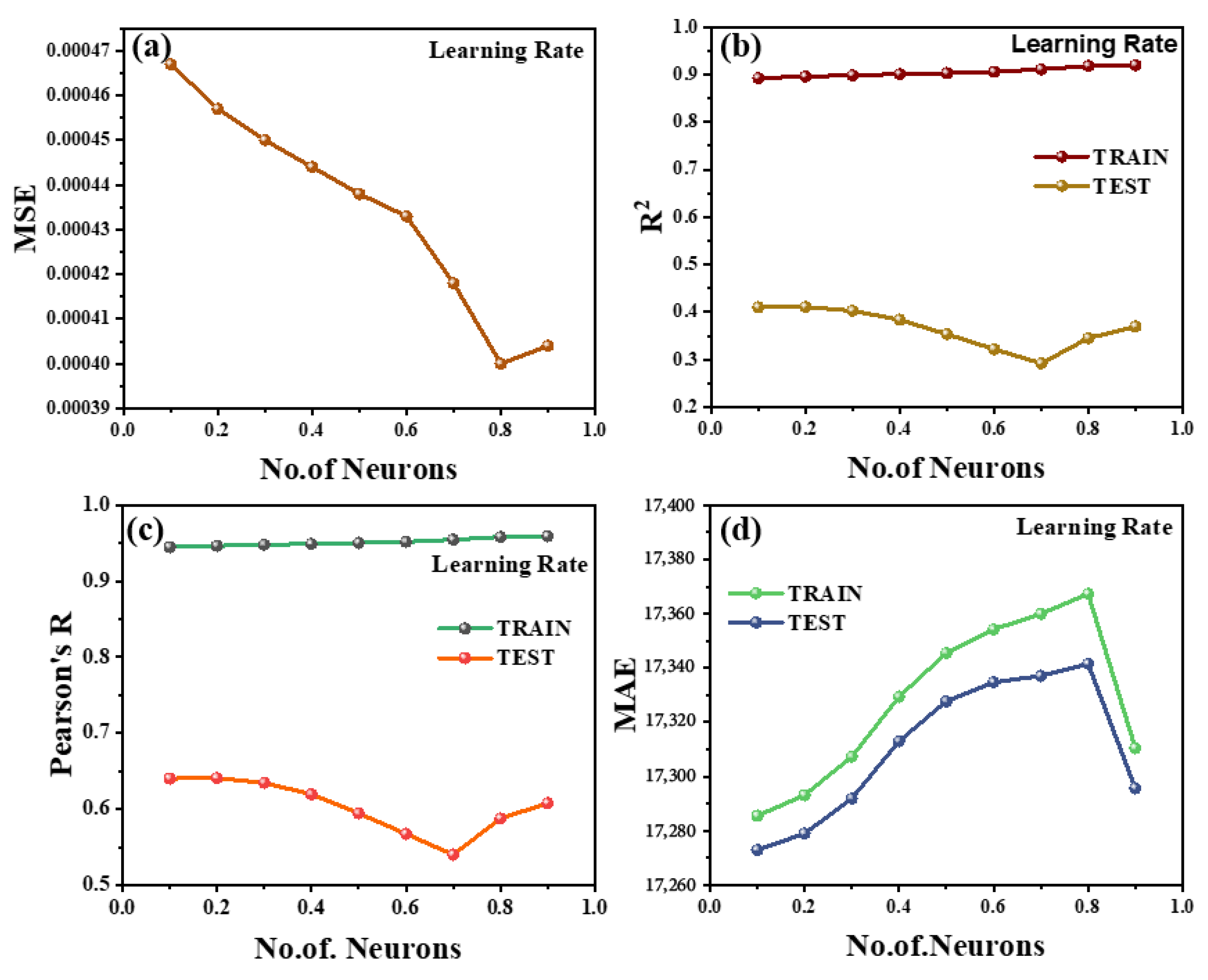
Figure 7a–d present the same metrics as functions of network size for different learning rates. Here, the learning rate of 0.3 demonstrates the most favorable performance. For example, at six neurons the MSE for a learning rate of 0.3 is ≈0.95 (Figure 7a), approximately 10–15% lower than a learning rate of 0.2 (≈1.05) and significantly lower than a learning rate of 0.5 (≈1.25). The MAE (Figure 7d) is ≈0.25 for a learning rate of 0.3 (vs. ≈0.27 at a learning rate of 0.2 and ≈0.32 at a learning rate of 0.5). The R2 and Pearson curves (Figure 7b,c) reach maximum values of approximately 0.84 and 0.91, respectively, for a learning rate of 0.3 (six neurons), exceeding the performance of all other tested configurations (e.g., R2 ≈ 0.80, r ≈ 0.88 for a learning rate of 0.2) and substantially outperforming the near-zero R2 (and r≈0.60) for a learning rate of 0.5. An R2 value of approximately 0.84 corresponds to about 84% variance explained, and r ≈ 0.91 indicates very strong correlation. These figures show that a learning rate of 0.3 achieves the fastest convergence and lowest prediction error, whereas an excessively large learning rate (0.5) causes the loss to plateau at high values (network fails to converge) and a very low learning rate (0.1) results in slow convergence behavior (higher steady-state loss).
Across hidden-layer sizes, the learning rate of 0.3 consistently produces superior training dynamics: error drops rapidly up to ~six neurons then plateaus, while R2 peaks and then marginally declines. By contrast, a learning rate of 0.1 demonstrates a steady but slow error decrease with size (underfitting due to slow learning), and a learning rate of 0.5 remains flat with poor performance metrics (high error, low R2 regardless of size), consistent with divergence from an overly large step size. Thus, Figure 7 confirms that a learning rate of 0.3 achieves a favorable trade-off: it converges quickly without oscillation, whereas too-low or too-high rates lead to typical issues of underfitting and gradient overshooting, respectively.
Overall, the 9-6-6-1 (two-layer) network trained for 15,000 iterations with momentum = 0.4 and learning rate = 0.3 as the optimal configuration was identified. This setup achieves high predictive accuracy (high R2 and Pearson correlation coefficient values) while maintaining low error on unseen data. It is sufficiently complex to fit the data (achieving low error) without overfitting. The single-layer networks exhibited insufficient representational capacity (yielding lower R2 and erratic test errors), while the three-layer networks were overly complex and exhibited elevated validation error. These findings align with established machine learning principles: increasing hidden units can improve training fit but raise overfitting risk, and the optimal model balances training performance and generalization accuracy on training and test data. Therefore, the combination of the 9-6-6-1 architecture, extended training iterations, and properly tuned momentum and learning rate yields the most robust and accurate predictive performance for our modeling task.

3.5. Comparison Between ANN Models with Analytical Equation Predictions

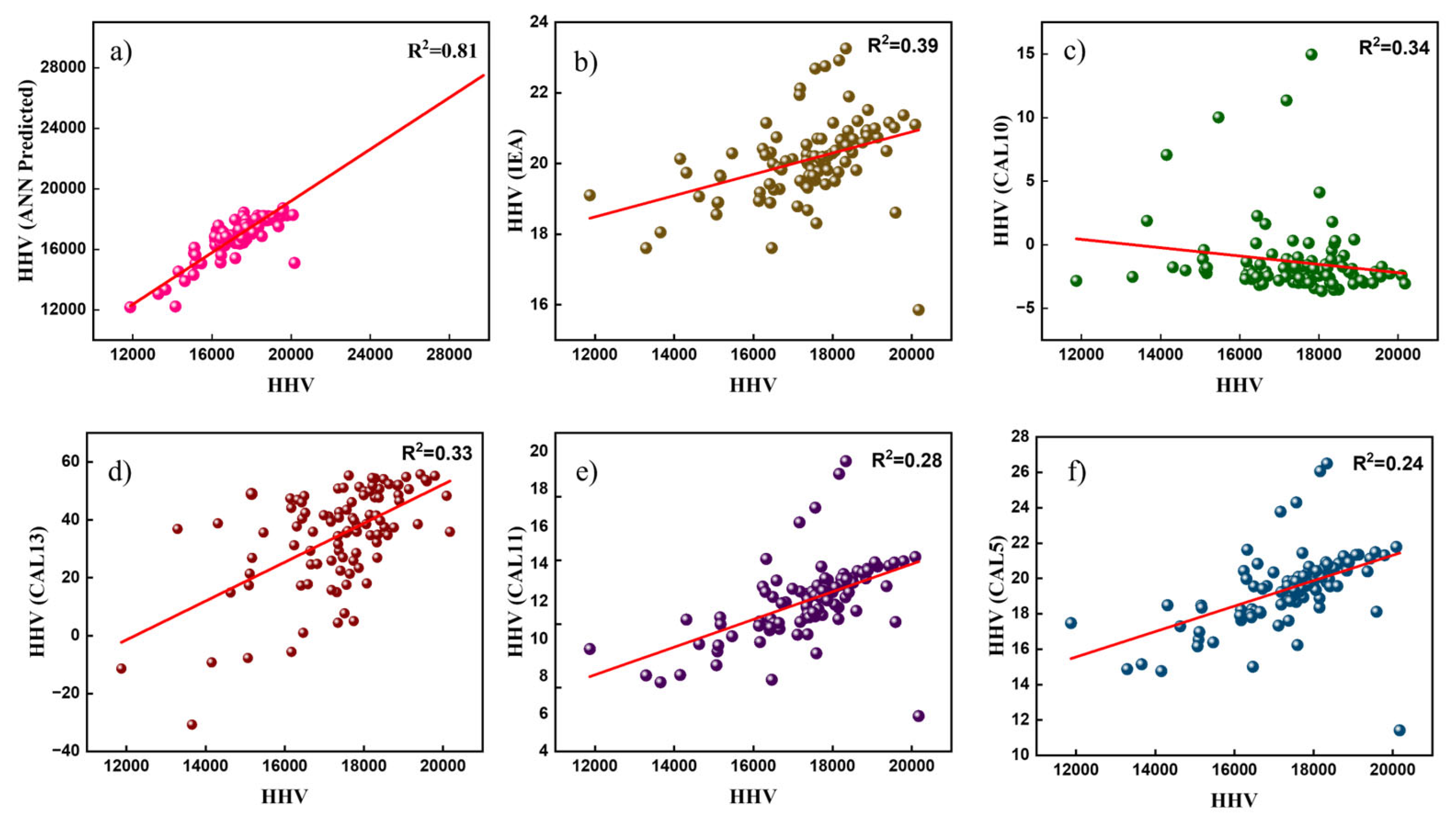
Figure 8 represents the scatter plots of the predicted vs. the measured HHV for Spanish biomass samples, comparing the ANN model (panel a) with five literature-based analytical equations: IEA (b), CAL10 (c), CAL13 (d), CAL11 (e), and CAL5 (f). Each panel reports the regression coefficient R2 for its fit to the 1:1 reference line. The ANN predictions (a) cluster tightly around the diagonal, indicating high accuracy and minimal bias (R2 = 0.81). By contrast, the analytical models (b–f) exhibit progressively wider scatter and lower R2 (IEA: 0.39; CAL10: 0.34; CAL13: 0.33; CAL11: 0.28; CAL5: 0.24), with IEA performing best among them but still deviating substantially from the ideal line. The results clearly indicate that the ANN output is a better fit for the measured values than the simpler formulae.
The ANN’s nonlinear regression demonstrates substantially improved performance in capturing complex biomass–HHV correlations compared to conventional analytical equations. In Figure 8a, the data points align closely with the 1:1 reference line, reflecting minimal residual error in the ANN predictions. By contrast, Figure 8b–f show that each analytical equation yields dispersed predictions with higher residual error, resulting in significant errors, particularly for compositions that deviate from the calibration dataset. This behavior is consistent with prior observations that biomass HHV relationships are inherently nonlinear, so advanced models, like neural networks, can learn the underlying patterns more robustly [13]. The literature-based equations, by relying on simpler (often linear) formulations, fail to capture the complexity of the true HHV dependence and thus generalize poorly across heterogeneous samples [22]. Indeed, even the IEA equation, which attains the highest R2 among the analytical group, exhibits substantial deviation from the measured values, while the CAL10 → CAL5 equations exhibit progressive decline in R2 and increased variance in prediction. These trends are reinforced by the supplementary analyses (Figures S3–S7). Table 3 summarizes the top 15 analytical equations and their corresponding R2 values, illustrating that many published HHV correlations fail to generalize across diverse biomass types. The remaining analytical equations are provided in Table S2. Overall, the ANN model’s strong alignment with the 1:1 line and high R2 underscores its ability to learn complex, multi-variable patterns (e.g., interactions of proximate/ultimate components) that the linear equations cannot. These findings confirm that a data-driven ANN approach provides a robust, generalizable predictor of the biomass HHV, offering significantly improved accuracy over traditional analytical formulas.
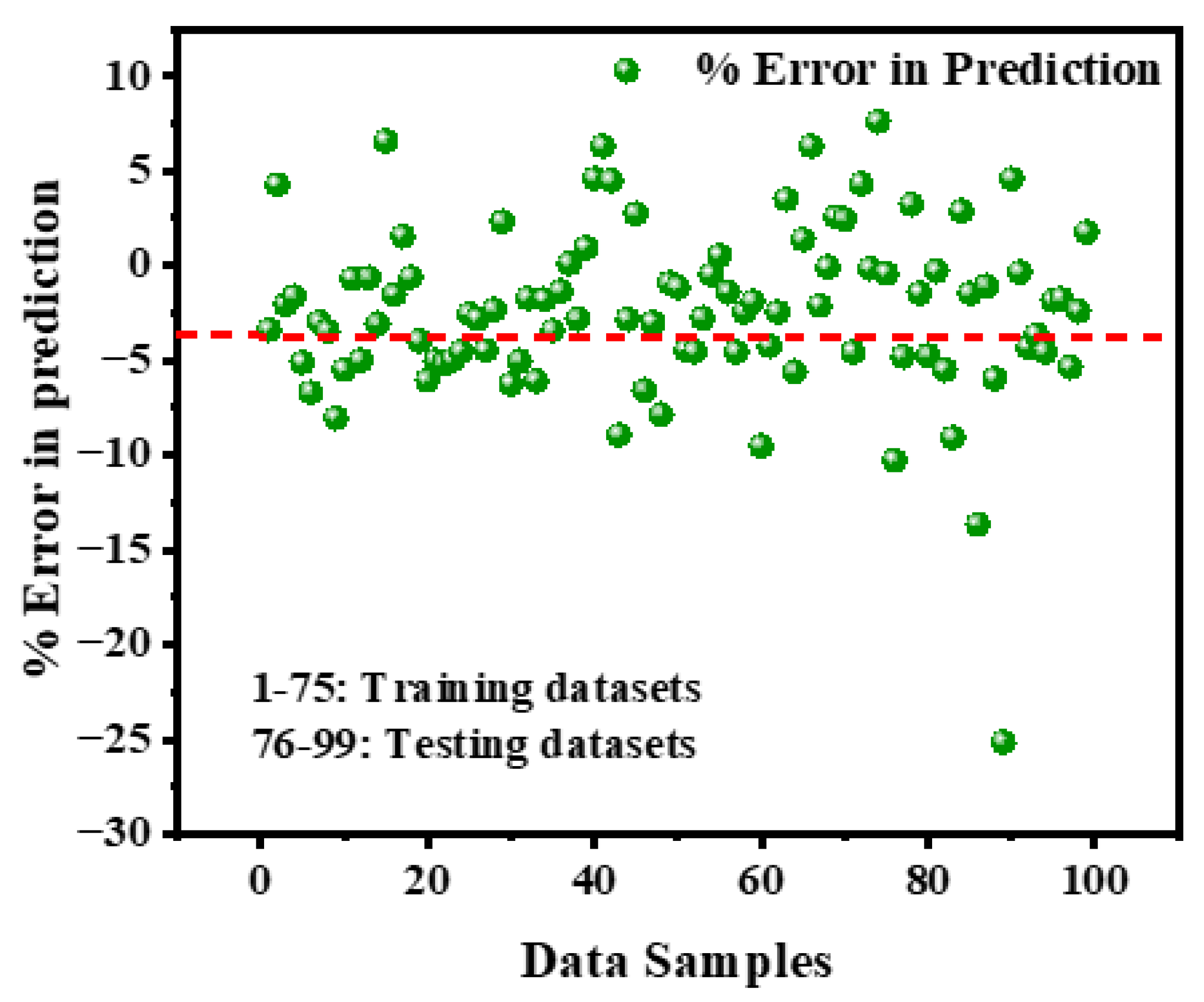
Figure 9 presents the percent prediction error for all 99 biomass samples, with the first 75 representing the training set and the remaining 24 the testing set. The average error across all samples is –2.37%, indicating a slight overall underprediction. In the training set, errors are generally centered near zero and mostly fall within ±8%, reflecting good model fit. The testing set shows slightly more variability, with most errors within ±12%, but no clear trend of systematic over- or underestimation is observed. Overall, the model demonstrates consistent and acceptable predictive performance across both training and unseen data.
The neural network’s much higher accuracy can be traced to its ability to fit complex, nonlinear relationships among the compositional inputs, whereas most analytical HHV correlations are simple linear formulas calibrated to limited data sets. Jenkins et al. (1998) explicitly observed that coal-derived formulas typically do not perform well at predicting the HHV for biomass [32]. Likewise, Mateeva et al. (2022) [33] noted that, although hundreds of empirical HHV correlations exist, those fitted to one biomass type may fail to provide accurate results for others. Crucially, the standard correlations we tested were often developed from global or coal-biased datasets and so were not tuned to Spain’s local biofuel mix. For example, Pizarro et al. (2014) [14,15] reported Spanish HHV measurements for 100 samples spanning forest and agricultural residues, energy crops, and commercial fuels—a diversity of composition that generic equations do not capture. This mismatch helps explain why the published formulas yield very low R2 on our data. We also stress that the ANN’s improved performance depends on having representative training data: an ANN trained on a narrow or homogeneous set may not generalize to feedstocks outside that domain. In other words, while our ANN clearly outperforms the generic correlations on the present Spanish samples, its predictive power beyond the learned domain would require careful validation with more diverse data.

3.6. Comparison with Multivariable Linear Regression

To compare the ANN model’s performance, a multivariable linear regression (MLR) model was built using the same nine input variables. On the test set, the MLR model achieved R2 ≈ 0.62, MAE ≈ 1.21 MJ/kg, and MSE ≈ 2.56 MJ2/kg2. These values are notably worse than those achieved by the ANN model (R2 ≈ 0.81, MAE ≈ 0.77 MJ/kg), highlighting the ANN’s advantage in modeling nonlinear relationships inherent in biomass HHV prediction.

3.7. Generalization Performance on Non-Spanish Biomass Samples

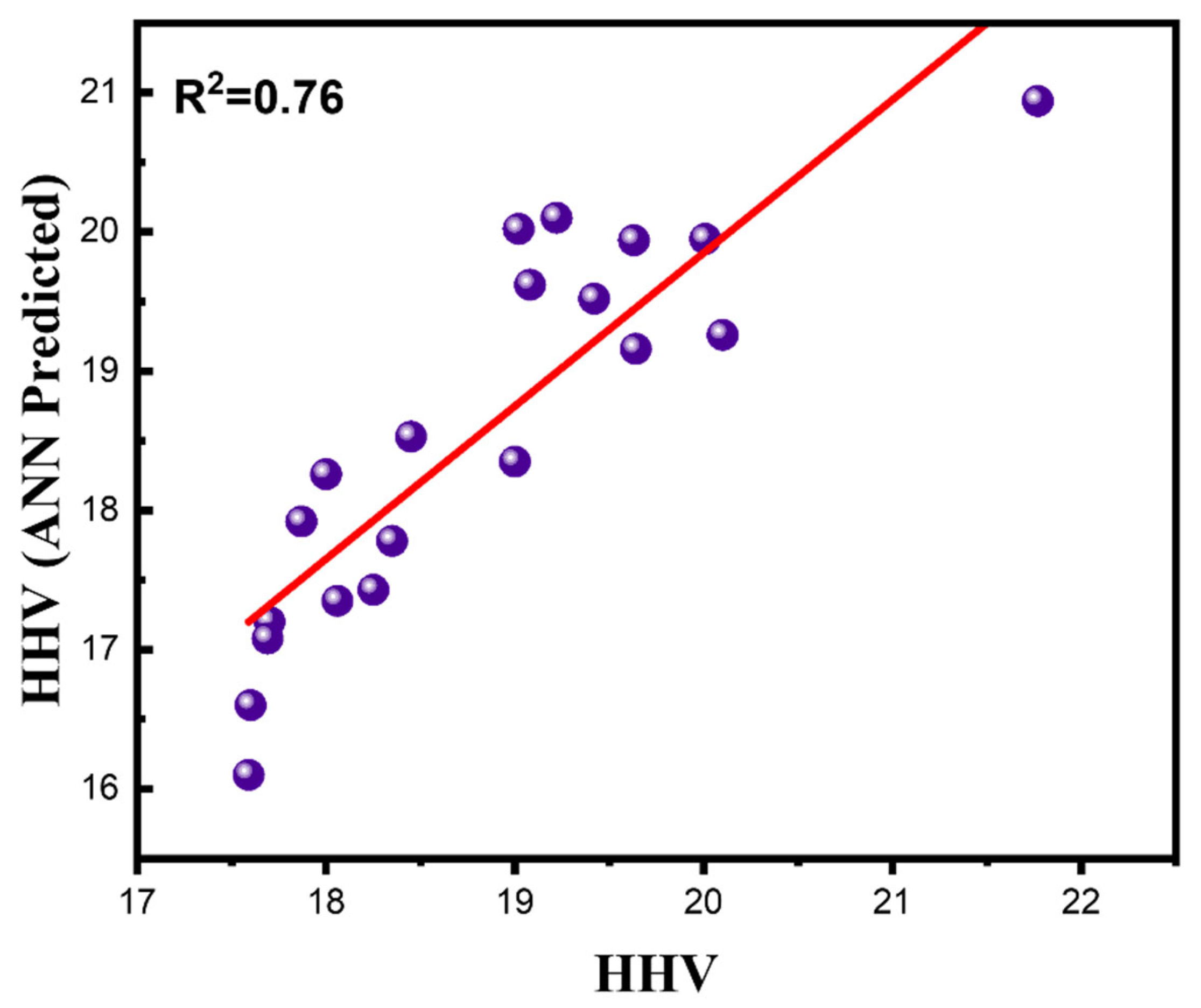
Figure 10 shows a scatter plot of the predicted higher heating values (HHV) for the 20 external (non-Spanish) biomass samples compared to the actual HHV. The data points are very close to the unity (1:1) line, indicating the strong correlation between the ANN’s predictions and the actual calorific values. These samples—detailed in Supplementary Table S3—span a broad range of fuel types, including commercial fuel woods, industrial residues, energy crops, and cereal crop residues. Each sample was fully characterized by standard proximate (moisture, ash, volatile matter, fixed carbon) and ultimate (C, H, O, N, S) analyses before applying the model. For this validation set, the ANN achieved a coefficient of determination R2 ≈ 0.76, reflecting a very strong linear correlation between the predicted and the observed HHV. The average absolute prediction error is only about 0.56 MJ·kg−1 (roughly 3–4% of the HHV), and most individual deviations are quite small—no systematic bias is evident (one sample shows a somewhat larger error). In short, the high R2 and low errors from this varied data show that the ANN is strong; the model remains accurate for different types of biomass beyond the original Spanish training set, proving it can effectively predict for new feedstock types.

3.8. Index of Relative Importance (IRI) for the Estimation of the Qualitative Influence of Input Variables on Output

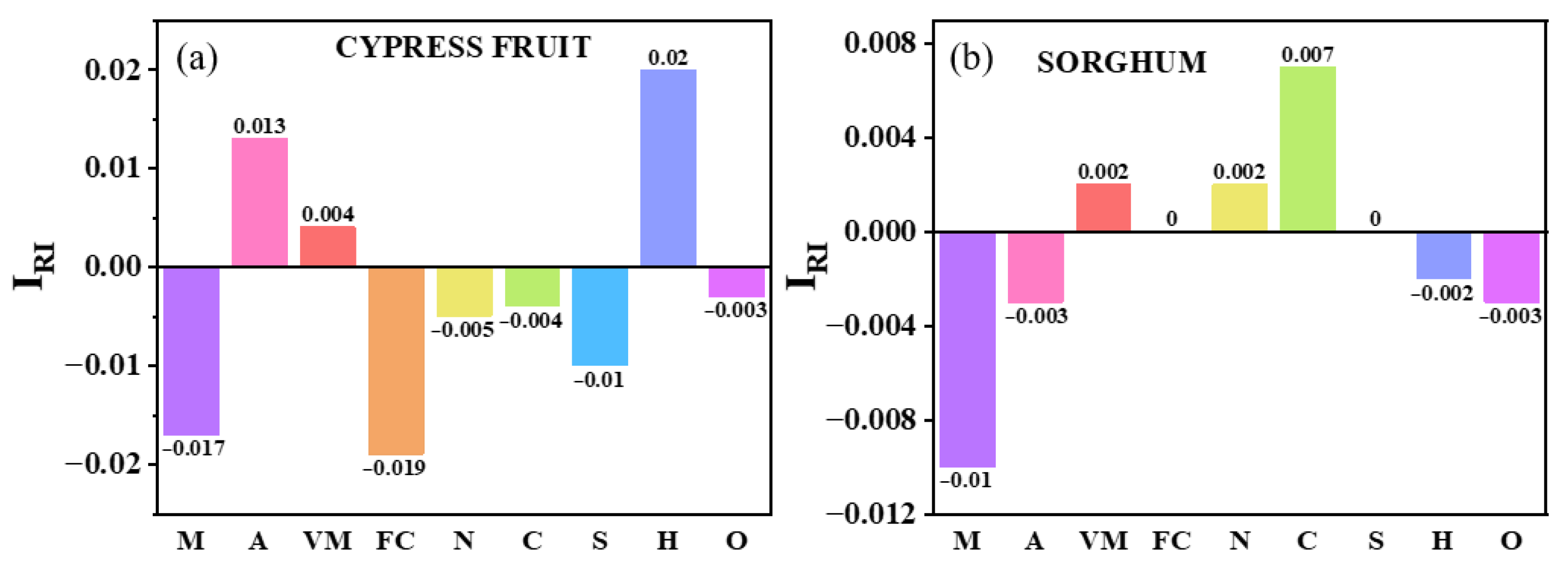
The IRI (Index of Relative Importance) analysis in Figure 11 shows that, for the Cypress sample (Figure 11a), hydrogen (H) has the largest positive IRI (+0.020) and fixed carbon (FC) the largest negative (–0.019). The model thus predicts a higher HHV when H is higher and a lower HHV when FC is higher, which appears counter-intuitive for FC. In fuel chemistry this makes sense: H-rich fuels yield more energy, whereas inert carbon (fixed C) yields less.
Dulong’s formula (HHV ≈ 33.87·C + 122.3·(H − O/8) + 9.4·S) shows both C and especially H contribute positively to HHV, and reviews confirm that carbon–hydrogen compounds are much more energetic than oxygenated materials [34,35]. Thus, the model’s high IRI for H agrees with theory (each unit of H yields large heat when oxidized). The negative IRI for FC, however, is likely to reflect data interdependencies rather than a true negative physics. In our data, a high FC value often coincides with lower volatile matter or higher ash content. When features are collinear, a model can obtain the same information from a correlated feature, effectively sharing predictive power.
More generally, this means that the network tends to attribute combustion energy to other correlated inputs, so an isolated increase in FC looks like a shift to a mixture with a lower HHV. Importantly, we interpret the IRI values as descriptive feature sensitivities, not mechanistic laws. This study emphasizes that these interpretations describe the model’s learned associations rather than establishing causation—correlation does not imply causation. For example, prior regression and Pearson studies also found H and C to be the strongest positive correlates of the HHV, with ash, O (and moisture) negative [36].
For the sorghum sample (Figure 11b), carbon (C) has the highest IRI (0.007) and moisture (M) the lowest (–0.010). The model thus sees higher C as boosting HHV and higher moisture as suppressing it. Again, this aligns with chemistry: carbon oxidation releases energy, so an increase in carbon is associated with a higher HHV in our model’s context. Moisture is dilutive (water vaporization consumes heat), which in the model’s view corresponds to our data showing samples with more moisture to have a lower HHV. Indeed, studies have reported a clear negative linear relationship between moisture and HHV: fuel HHV is negatively correlated with water and decreases as moisture increases [16,37]. The IRI results capture this: moisture’s negative IRI is the strongest suppressor of HHV in sorghum. Parallel MLR/Pearson analyses similarly identify C and H as the main positive drivers and moisture/ash as the negative drivers. This reflects the model’s sensitivity to inputs rather than physical causation. In other words, the sorghum model identifies C as the key positive predictor and moisture as the key negative predictor, consistent with known fuel chemistry, but these are learned correlations, not proof of cause–effect.
Looking across all samples (Figure S8), carbon and hydrogen are universally the strongest positive IRI influences on the HHV, while moisture and ash carry the largest negative IRI. Fixed carbon generally has little or often a slight negative effect, and volatile matter is relatively unimportant. This matches prior findings (e.g., C + H ≈ 52% of HHV influence vs. only 2–3% for N, O, VM). In short, H and C have the highest positive IRI, whereas moisture and ash have large negative IRI, with FC contributing little (often negative). This suggests that fixed carbon is not an independent driver of the HHV in our models: its negligible or negative IRI likely results from collinearity with other fuel components (high FC tends to coincide with mixtures of lower heating value). Minor variations occur sample-to-sample, but no sample overturns these overall patterns.
It is emphasized that the signs of IRI simply indicate the model’s learned associations (feature influences on the output), not actual causation. Higher C and H do correlate with a higher HHV (since C–H fuels are energetic), and higher moisture or inert content with a lower HHV (water and ash dilute energy). Framing our discussion via Pearson correlation and IRI provides an interpretable view of what the model has learned, not a proof of the underlying physics. In other words, each positive/negative IRI shows how changing that input shifts the predicted HHV, but correlation does not imply causation. The positive IRI for C and H and negative IRI for moisture/ash thus align with chemical intuition, but, ultimately, they reflect statistical patterns in the data and the model’s sensitivity to them, rather than a causal inference.

3.9. GUI Implementation

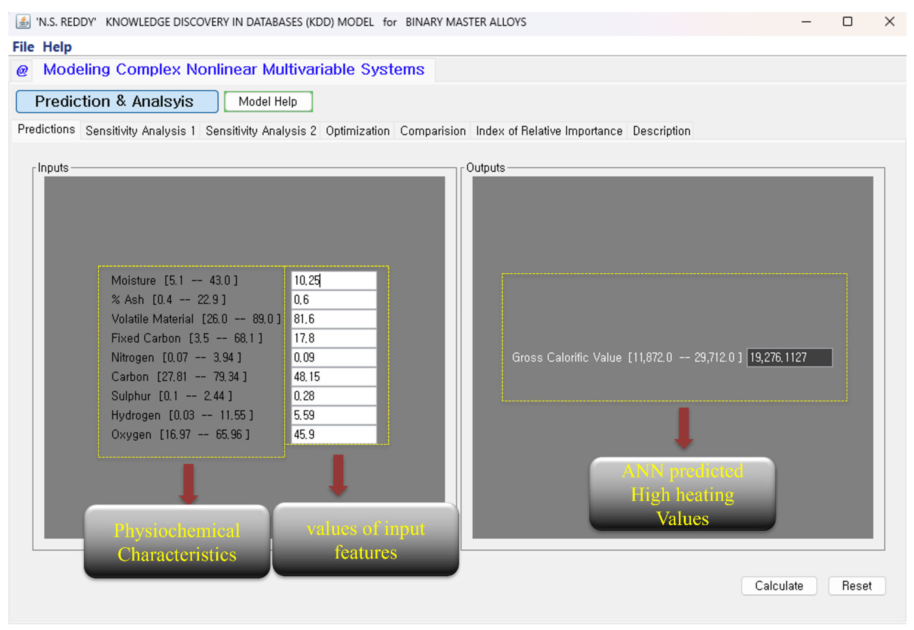
Figure 12 illustrates the custom ANN-based biomass fuel prediction tool’s user interface. The layout is divided into an input panel (left) and an output panel (right). The input panel contains clearly labeled fields for the nine physicochemical parameters used by the model: Moisture, Ash, Volatile Matter, Fixed Carbon, Nitrogen, Carbon, Sulfur, Hydrogen, and Oxygen. The interface allows for the manual input of values for each parameter (e.g., by typing in measured percentages or fractions). A ‘Calculate’ button initiates the trained neural network, and the output panel then displays the resulting gross calorific value (HHV). Thus, researchers or practitioners can input proximate/ultimate analysis data and obtain the ANN’s HHV estimate without requiring programming skills. The user interface is designed for clarity and ease of use. The names of the input fields (and units, if needed) are on each field, and the parameters are organized in a way that is logical (for example, proximal analysis components versus elemental composition). The results are indicated explicitly in a ‘Predicted HHV’ box/section. The GUI is designed with the end-user in mind, whereby the platform enables the user to enter fuel data and obtain half-hourly HHV predictions swiftly without having to grasp the underlying concepts related to the model.
Aside from critical predictive capabilities, the interface also offers more complex analytical modules for an extensive analysis of the biomass data. For instance, an optimization module will systematically find the best combination of input values (within permissible ranges) that maximizes the predicted HHV, thus serving users in determining how the feedstock can potentially be improved in quality. Also, comparison tools are provided so that various biomass samples might be studied simultaneously: a user may enter and record different sets of parameters to view the predicted HHVs side by side; meanwhile, a set of conventional empirical HHV correlations could also be given as output on the same inputs for reference, highlighting the superior predictive power of the ANN model against classical methods. The actual implementation uses a static trained ANN model, but, at the architectural level, the tool is destined for future extensions. Incorporating new biomass types and other data may require retraining or fine-tuning the networks, while further improvements may include establishing an automatic model-update pipeline so that model applicability may enhance the development of feedstocks. Current biomass data are used either for retraining an existing artificial neural network or for gradually improving it so that the model may accommodate potential unknown feedstock types. This approach may be refined through an update pipeline that regularly retrains the network with new data to keep the model relevant and accurate with an ever-expanding database. The GUI has a modular design so that newer or modified input parameters can be incorporated in subsequent versions without taxing the interface with additional chemical components or feedstock attributes. The tool facilitates a biomass energy assessment in an accessible manner, including live HHV estimations and scenario analysis, thereby supporting research and decision-making processes more efficiently.

4. Conclusions

In conclusion, the ANN model accurately predicts the HHV of diverse Spanish biomass samples from routine compositional analyses. Proximate data were collected (moisture, ash, volatile matter, fixed carbon) and ultimate (C, H, N, S, O) data for 99 biomass fuels and trained on a 9-6-6-1 backpropagation network (with logistic activation) for 15,000 epochs (learning rate = 0.3, momentum = 0.4). The optimized ANN achieved a strong predictive performance; on the test set, it reached R2 ≈ 0.81. This performance significantly surpasses that of conventional analytical HHV correlations from the literature, demonstrating that the ANN effectively captures the complex, nonlinear relationships between biomass composition and energy content that fixed formulas cannot.
A feature-importance analysis (using the Index of Relative Importance) confirmed chemically intuitive trends: fuels richer in carbon or hydrogen have higher predicted HHV, whereas higher moisture, ash, or oxygen content lowers it. These results align with classical fuel-chemistry principles and suggest and demonstrate that the model captures meaningful physical patterns. Additionally, a user-friendly graphical interface was developed, allowing practitioners to input a biomass’s proximate and elemental values and instantly obtain the ANN’s HHV estimate. Overall, the ANN model provides an accurate and efficient tool for rapid HHV estimation. However, this study has certain limitations: the dataset of 99 samples is relatively small and regionally specific to Spanish biomass, which may limit the model’s generalizability to other feedstock types or geographic regions. However, the model’s improved accuracy and its ability to handle heterogeneous feedstocks provide greater flexibility and reliability in biomass energy planning and decision support. For Instance, in both academic research and industrial energy assessment contexts, the interface allows for quick comparison and selection of biomass feedstocks based on the ANN’s HHV predictions, informing fuel-blending decisions and resource allocation, thereby contributing to more efficient bioenergy systems and low-carbon fuel utilization.

Supplementary Materials

The following supporting information can be downloaded at: https://www.mdpi.com/article/10.3390/en18154067/s1, Figure S1: Training behavior graph of 1 layer; Figure S2: Training behavior graph of 3 layers; Figure S3: Comparison between the developed ANN with traditional empirical equations; Figure S4: Comparison between the developed ANN with traditional empirical equations; Figure S5: Comparison between the developed ANN with traditional empirical equations; Figure S6: Comparison between the developed ANN with traditional empirical equations; Figure S7: Comparison between the developed ANN with traditional empirical equations for WIL; Figure S8: Relative Importance Index of Physicochemical Variables on (a–c) high values of higher heating value, (d–f) average values of higher heating value, and (g–i) low values of higher heating value; Table S1: Raw data used to generate the ANN proposed empirical equations; Table S2: Analytical equations based on proximate analysis data selected from the literature; Table S3: Actual vs. Predicted HHV for non-Spanish Biomass Samples [5,11,26,27,28,29,31,35,38,39,40,41,42,43,44,45,46,47,48,49,50,51,52,53,54,55,56,57,58,59,60].

Author Contributions

A.J.: methodology, formal analysis, visualization, writing—original draft. F.O.M.: methodology, investigation, data curation, writing—original draft. M.I. validation, writing—review and editing. S.Y.K.: data curation, resources, supervision, writing—review and editing. N.G.S.R.: software, conceptualization, validation, supervision, writing—review and editing. All authors have read and agreed to the published version of the manuscript.

Funding

This work was supported by the Learning & Academic Research Institution for Masters’s, PhD students, and Postdocs (LAMP) Program of the National Research Foundation of Korea (NRF) grant funded by the Ministry of Education (No. RS-2023-00301974). This work was also supported by the Global University 30 Project fund of Gyeongsang National University in 2025.

Data Availability Statement

The original contributions presented in this study are included in the article/Supplementary Materials. Further inquiries can be directed to the corresponding authors.

Conflicts of Interest

The authors declare no competing interests.

References

  1. Mignogna, D.; Szabó, M.; Ceci, P.; Avino, P. Biomass Energy and Biofuels: Perspective, Potentials, and Challenges in the Energy Transition. Sustainability 2024, 16, 7036. [Google Scholar] [CrossRef]
  2. Perea-Moreno, M.-A.; Samerón-Manzano, E.; Perea-Moreno, A.-J. Biomass as Renewable Energy: Worldwide Research Trends. Sustainability 2019, 11, 863. [Google Scholar] [CrossRef]
  3. Kujawska, J.; Kulisz, M.; Oleszczuk, P.; Cel, W. Improved Prediction of the Higher Heating Value of Biomass Using an Artificial Neural Network Model Based on the Selection of Input Parameters. Energies 2023, 16, 4162. [Google Scholar] [CrossRef]
  4. Shehab, M.; Stratulat, C.; Ozcan, K.; Boztepe, A.; Isleyen, A.; Zondervan, E.; Moshammer, K. A comprehensive analysis of the risks associated with the determination of biofuels’ calorific value by bomb calorimetry. Energies 2022, 15, 2771. [Google Scholar] [CrossRef]
  5. Noushabadi, A.S.; Dashti, A.; Ahmadijokani, F.; Hu, J.; Mohammadi, A.H. Estimation of higher heating values (HHVs) of biomass fuels based on ultimate analysis using machine learning techniques and improved equation. Renew. Energy 2021, 179, 550–562. [Google Scholar] [CrossRef]
  6. Qian, C.; Li, Q.; Zhang, Z.; Wang, X.; Hu, J.; Cao, W. Prediction of higher heating values of biochar from proximate and ultimate analysis. Fuel 2020, 265, 116925. [Google Scholar] [CrossRef]
  7. Aladejare, A.E.; Onifade, M.; Lawal, A.I. Application of metaheuristic based artificial neural network and multilinear regression for the prediction of higher heating values of fuels. Int. J. Coal Prep. Util. 2022, 42, 1830–1851. [Google Scholar] [CrossRef]
  8. Zhou, L.; Song, Y.; Ji, W.; Wei, H. Machine learning for combustion. Energy AI 2022, 7, 100128. [Google Scholar] [CrossRef]
  9. Ishtiaq, M.; Tiwari, S.; Panigrahi, B.B.; Seol, J.B.; Reddy, N.S. Neural Network-Based Modeling of the Interplay between Composition, Service Temperature, and Thermal Conductivity in Steels for Engineering Applications. Int. J. Thermophys. 2024, 45, 1–31. [Google Scholar] [CrossRef]
  10. Pattanayak, S.; Loha, C.; Hauchhum, L.; Sailo, L. Application of MLP-ANN models for estimating the higher heating value of bamboo biomass. Biomass Convers. Biorefinery 2021, 11, 2499–2508. [Google Scholar] [CrossRef]
  11. Abdollahi, S.A.; Ranjbar, S.F.; Jahromi, D.R. Applying feature selection and machine learning techniques to estimate the biomass higher heating value. Sci. Rep. 2023, 13, 16093. [Google Scholar] [CrossRef] [PubMed]
  12. Güleç, F.; Pekaslan, D.; Williams, O.; Lester, E. Predictability of higher heating value of biomass feedstocks via proximate and ultimate analyses—A comprehensive study of artificial neural network applications. Fuel 2022, 320, 123944. [Google Scholar] [CrossRef]
  13. Aghel, B.; Yahya, S.I.; Rezaei, A.; Alobaid, F. A Dynamic Recurrent Neural Network for Predicting Higher Heating Value of Biomass. Int. J. Mol. Sci. 2023, 24, 5780. [Google Scholar] [CrossRef]
  14. García, R.; Pizarro, C.; Lavín, A.G.; Bueno, J.L. Spanish biofuels heating value estimation. Part I: Ultimate analysis data. Fuel 2014, 117, 1130–1138. [Google Scholar] [CrossRef]
  15. García, R.; Pizarro, C.; Lavín, A.G.; Bueno, J.L. Spanish biofuels heating value estimation. Part II: Proximate analysis data. Fuel 2014, 117, 1139–1147. [Google Scholar] [CrossRef]
  16. García, R.; Pizarro, C.; Lavín, A.G.; Bueno, J.L. Characterization of Spanish biomass wastes for energy use. Bioresour. Technol. 2012, 103, 249–258. [Google Scholar] [CrossRef]
  17. Demirbas, A. Combustion characteristics of different biomass fuels. Prog. Energy Combust. Sci. 2004, 30, 219–230. [Google Scholar] [CrossRef]
  18. Bishop, C.M.; Nasrabadi, N.M. Pattern Recognition and Machine Learning; Springer: Singapore, 2006; Volume 4. [Google Scholar]
  19. Li, J.; Yuan, X.; Kuruoglu, E.E. Exploring Weight Distributions and Dependence in Neural Networks with α-Stable Distributions. IEEE Trans. Artif. Intell. 2024, 5, 5519–5529. [Google Scholar] [CrossRef]
  20. Zhang, J.; Li, H.; Sra, S.; Jadbabaie, A. Neural network weights do not converge to stationary points: An invariant measure perspective. In Proceedings of the International Conference on Machine Learning, PMLR, Baltimore, MD, USA, 17–23 July 2022. [Google Scholar]
  21. Ismailov, V.E. A three layer neural network can represent any multivariate function. J. Math. Anal. Appl. 2023, 523, 127096. [Google Scholar] [CrossRef]
  22. Demirbaş, A. Calculation of higher heating values of biomass fuels. Fuel 1997, 76, 431–434. [Google Scholar] [CrossRef]
  23. Graboski, M.; Bain, R. Properties of biomass relevant to gasification. In Biomass Gasification-Principles and Technology; Noyes Data Corporation: Park Ridge, NJ, USA, 1981; pp. 41–69. [Google Scholar]
  24. Adapa, P.K.; Adapa, P.K.; Schoenau, G.J.; Tabil, L.G.; Sokhansanj, S.; Crerar, B. Pelleting of fractionated alfalfa products. In Proceedings of the 2003 ASAE Annual Meeting, American Society of Agricultural and Biological Engineers, Las Vegas, NV, USA, 27–30 July 2003. [Google Scholar]
  25. Callejón-Ferre, A.; Velázquez-Martí, B.; López-Martínez, J.; Manzano-Agugliaro, F. Greenhouse crop residues: Energy potential and models for the prediction of their higher heating value. Renew. Sustain. Energy Rev. 2011, 15, 948–955. [Google Scholar] [CrossRef]
  26. Kathiravale, S. Modeling the heating value of Municipal Solid Waste☆. Fuel 2003, 82, 1119–1125. [Google Scholar] [CrossRef]
  27. Abu-Qudais, M.; A Abu-Qdais, H. Energy content of municipal solid waste in Jordan and its potential utilization. Energy Convers. Manag. 2000, 41, 983–991. [Google Scholar] [CrossRef]
  28. Meraz, L.; Domínguez, A.; Kornhauser, I.; Rojas, F. A thermochemical concept-based equation to estimate waste combustion enthalpy from elemental composition☆. Fuel 2003, 82, 1499–1507. [Google Scholar] [CrossRef]
  29. Sheng, C.; Azevedo, J. Estimating the higher heating value of biomass fuels from basic analysis data. Biomass Bioenergy 2005, 28, 499–507. [Google Scholar] [CrossRef]
  30. Mason, D.M.; Gandhi, K. Formulas for Calculating the Heating Value of Coal and Coal Char: Development, Tests, and Uses; No. CONF-800814-25; Institute of Gas Technology: Chicago, IL, USA, 1980. [Google Scholar]
  31. Channiwala, S.A.; Parikh, P.P. A unified correlation for estimating HHV of solid, liquid and gaseous fuels. Fuel 2002, 81, 1051–1063. [Google Scholar] [CrossRef]
  32. Jenkins, B.M.; Baxter, L.L.; Miles, T.R., Jr.; Miles, T.R. Combustion properties of biomass. Fuel Process. Technol. 1998, 54, 17–46. [Google Scholar] [CrossRef]
  33. Matveeva, A.; Bychkov, A. How to train an artificial neural network to predict higher heating values of biofuel. Energies 2022, 15, 7083. [Google Scholar] [CrossRef]
  34. Brandić, I.; Pezo, L.; Voća, N.; Matin, A. Biomass Higher Heating Value Estimation: A Comparative Analysis of Machine Learning Models. Energies 2024, 17, 2137. [Google Scholar] [CrossRef]
  35. Daskin, M.; Erdoğan, A.; Güleç, F.; Okolie, J.A. Generalizability of empirical correlations for predicting higher heating values of biomass. Energy Sources Part A Recover. Util. Environ. Eff. 2024, 46, 5434–5450. [Google Scholar] [CrossRef]
  36. Yang, X.; Li, H.; Wang, Y.; Qu, L. Predicting higher heating value of sewage sludges via artificial neural network based on proximate and ultimate analyses. Water 2023, 15, 674. [Google Scholar] [CrossRef]
  37. Esteves, B.; Sen, U.; Pereira, H. Influence of chemical composition on heating value of biomass: A review and bibliometric analysis. Energies 2023, 16, 4226. [Google Scholar] [CrossRef]
  38. Thipkhunthod, P.; Pharino, C.; Kitchaicharoen, J.; Phungrassami, H. Predicting the heating value of sewage sludges in Thailand from proximate and ultimate analyses. Fuel 2005, 84, 849–857. [Google Scholar] [CrossRef]
  39. Callejón-Ferré, A.J.; López-Martínez, J.A.; Manzano-Agugliaro, F.; Díaz-Pérez, M. Energy potential of greenhouse crop residues in southeastern Spain and evaluation of their heating value predictors. Renew. Sustain. Energy Rev. 2011, 15, 948–955. [Google Scholar] [CrossRef]
  40. Chang, Y.F.; Chang, C.N.; Chen, Y.W. Multiple regression models for lower heating value of municipal solid waste in Taiwan. J. Environ. Manag. 2007, 85, 891–899. [Google Scholar] [CrossRef]
  41. Yin, C.Y. Prediction of higher heating value of biomass from proximate and ultimate analyses. Fuel 2011, 90, 1128–1132. [Google Scholar] [CrossRef]
  42. Cordero, T.; Marquez, F.; Rodriguez-Mirasol, J.; Rodriguez, J.J. Predicting heating values of lignocellulosics from proximate analysis. Fuel 2001, 80, 1567–1571. [Google Scholar] [CrossRef]
  43. Parikh, J.; Channiwala, S.A.; Ghosal, G.K. A correlation for calculating HHV from proximate analysis of solid fuels. Fuel 2005, 84, 487–494. [Google Scholar] [CrossRef]
  44. Majumder, A.K.; Jain, R.; Banerjee, S.; Barnwal, J.P. An approach for developing an analytical relation of the HHV from proximate analysis of coal. Fuel 2008, 87, 3077–3081. [Google Scholar] [CrossRef]
  45. Ahmaruzzaman, M. A review on the utilization of fly ash. Prog. Energy Combust. Sci. 2010, 36, 327–363. [Google Scholar] [CrossRef]
  46. Jiménez, L.; González, F. Thermal behaviour of lignocellulosic residues treated with phosphoric acid. Fuel 1991, 70, 947–950. [Google Scholar] [CrossRef]
  47. Goutal, M. Sur le pouvoir calorifique de la houille. Comptes Rendus L’académie Sci. 1902, 134, 477–479. [Google Scholar]
  48. Kucukbayrak, S.; Goksel, M.; Gok, S. Estimation of calorific values of Turkish lignites using neural networks and regression analysis. Fuel 1991, 70, 979–981. [Google Scholar] [CrossRef]
  49. Matsuoka, K.; Kuramoto, K.; Suzuki, Y. Modification of Dulong’s formula to estimate heating value of gas, liquid and solid fuels. Fuel Process Technol. 2016, 152, 399–405. [Google Scholar]
  50. Mason, D.M.; Gandhi, K. Formulas for heating value of coal and coal char. Fuel Process Technol. 1983, 7, 11–22. [Google Scholar] [CrossRef]
  51. Arvidsson, M.; Morandin, M.; Harvey, S. Biomass gasification-based syngas production for a conventional oxo synthesis plant-greenhouse gas emission balances and economic evaluation. J. Clean. Prod. 2015, 99, 192–205. [Google Scholar] [CrossRef]
  52. Skodras, G.; Grammelis, O.P.; Basinas, P.; Kakaras, E.; Sakellaropoulos, G. Pyrolysis and combustion characteristics of biomass and waste-derived feedstock. Ind. Eng. Chem. Res. 2006, 45, 3791–3799. [Google Scholar] [CrossRef]
  53. Brandic, I.; Pezo, L.; Bilandzija, N.; Peter, A.; Suric, J.; Voca, N. Comparison of Different Machine Learning Models for Modelling the Higher Heating Value of Biomass. Mathematics 2023, 11, 2098. [Google Scholar] [CrossRef]
  54. Lehtonen, E.; Anttila, P.; Hakala, K.; Luostarinen, S.; Lehtoranta, S.; Merilehto, K.; Lehtinen, H.; Maharjan, A.; Mäntylä, V.; Niemeläinen, O.; et al. An open web-based GIS service for biomass data in Finland. Environ. Model. Softw. 2024, 176, 105972. [Google Scholar] [CrossRef]
  55. Capareda, S.C. Sustainable Biochar for Water and Wastewater Treatment Comprehensive Biomass Characterization in Preparation for Conversion, 1st ed.; Mohan, D., Pittman, C.U., Mlsna, T.E., Eds.; Elsevier: Amsterdam, The Netherlands, 2022; pp. 1–37. [Google Scholar]
  56. Yahya, A.M.; Adeleke, A.A.; Nzerem, P.; Ikubanni, P.P.; Ayuba, S.; Rasheed, H.A.; Gimba, A.; Okafor, I.; Okolie, J.A.; Paramasivam, P. Comprehensive Characterization of Some Selected Biomass for Bioenergy Production. ACS Omega 2023, 8, 43771–43791. [Google Scholar] [CrossRef]
  57. Dashti, A.; Noushabadi, A.S.; Raji, M.; Razmi, A.; Ceylan, S.; Mohammadi, A.H. Estimation of biomass higher heating value (HHV) based on the proximate analysis: Smart modeling and correlation. Fuel 2019, 257, 115931. [Google Scholar] [CrossRef]
  58. Database for the Physico-Chemical Composition of (Treated) Lignocellulosic Biomass, Micro- and Macroalgae, Various Feedstocks for Biogas Production and Biochar. Available online: https://phyllis.nl/ (accessed on 1 July 2024).
  59. Simon, F.; Girard, A.; Krotki, M.; Ordoñez, J. Modelling and simulation of the wood biomass supply from the sustainable management of natural forests. J. Clean. Prod. 2021, 282, 124487. [Google Scholar] [CrossRef]
  60. Malhi, A.; Knapic, S.; Främling, K. Explainable Agents for Less Bias in Human-Agent Decision Making. In Proceedings of the Explainable, Transparent Autonomous Agents and Multi-Agent Systems: Second International Workshop (EXTRAAMAS 2020), Auckland, New Zealand, 9–13 May 2020. [Google Scholar]
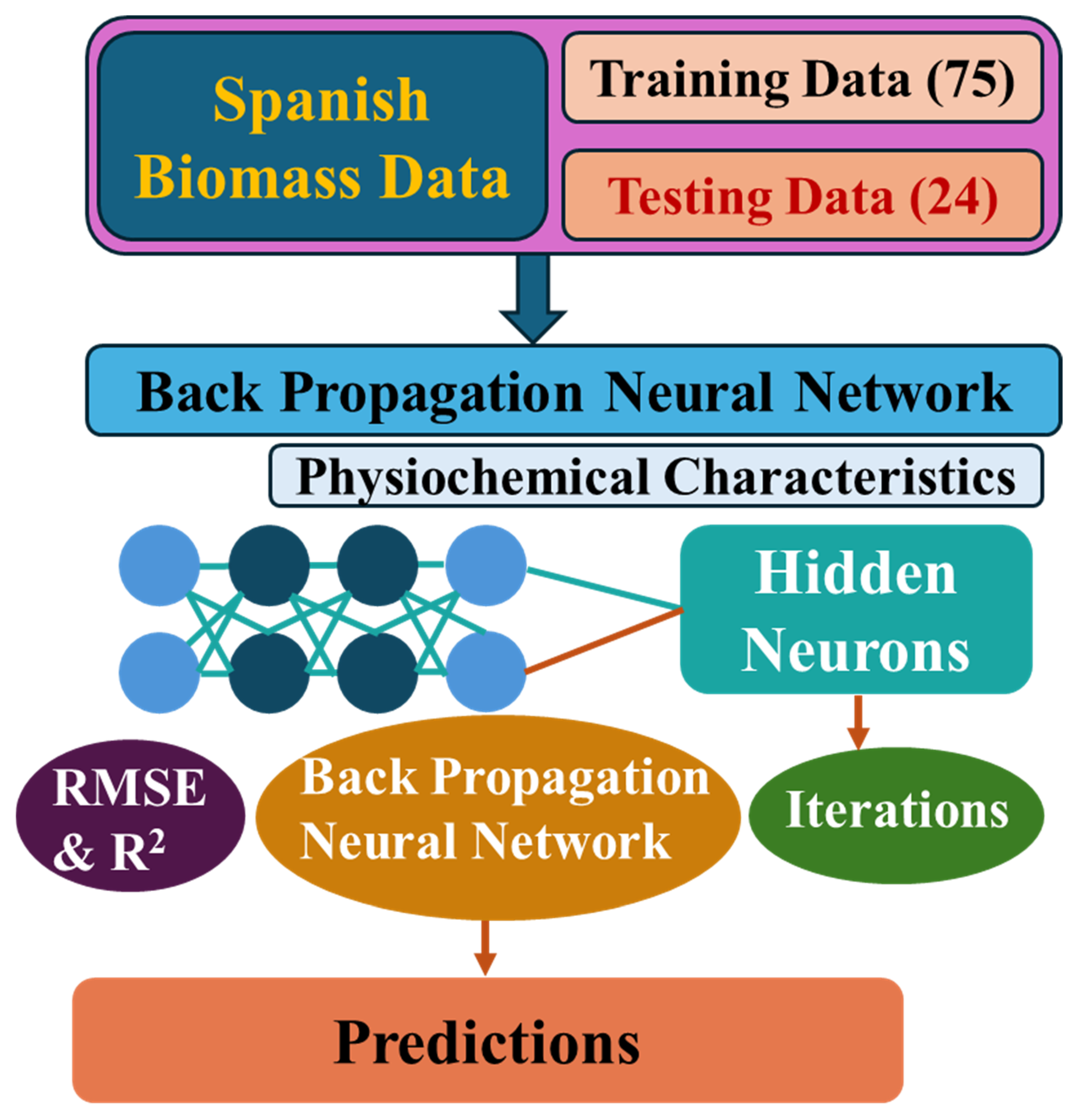
Figure 1. The ANN model development flow chart based on the backpropagation algorithm.
Energies 18 04067 g001
Figure 2. Visual correlation analysis of physicochemical properties and high heating value.
Energies 18 04067 g002
Figure 3. Correlation heat map of physicochemical parameters.
Energies 18 04067 g003
Figure 4. Distribution of the network weights in the ANN model: (a) 0 iterations; (b) 5000 iterations; (c) 10,000 iterations; (d) 15,000 iterations; (e) 20,000 iterations; (f) 30,000 iterations.
Energies 18 04067 g004
Figure 5. Training behavior graph of (9-6-6-1) layer: (a) mean squared error; (b) coefficient of determination (R2); (c) Pearson correlation coefficient; (d) main average error.
Energies 18 04067 g005
Figure 6. Training behavior graph of momentum rate: (a) mean squared error; (b) coefficient of determination (R2); (c) Pearson correlation coefficient; (d) main average error.
Energies 18 04067 g006
Figure 7. Training behavior graph of Learning Rate: (a) mean squared error; (b) coefficient of determination (R2); (c) Pearson correlation coefficient; (d) main average error.
Energies 18 04067 g007
Figure 8. Comparison between the developed ANN with Analytical equations: (a) Equation (1); (b) Equation (2); (c) Equation (3); (d) Equation (4); (e) Equation (5); (f) Equation (6). The 1:1 reference line (shown in red) represents perfect prediction accuracy.
Energies 18 04067 g008
Figure 9. Percentage prediction error across all 99 biomass samples. The x-axis represents sample index (1–75: training, 76–99: testing), and the y-axis shows the prediction error as a percentage of actual HHV. The red dashed line represents the mean percentage error across all samples, serving as a reference for overall model bias.
Energies 18 04067 g009
Figure 10. Prediction of the HHV for 20 external biomass samples from the optimized model. The red solid line represents the 1:1 reference line, indicating perfect prediction. Data points closer to this line signify better model accuracy.
Energies 18 04067 g010
Figure 11. Index of Relative Importance (IRI): (a) cypress fruit, (b) sorghum.
Energies 18 04067 g011
Figure 12. GUI interface developed for ANN-based HHV prediction from user-specified biomass inputs.
Energies 18 04067 g012
Table 1. Descriptive statistics (min, mean, max, std. dev.) of the nine input variables used to predict the HHV (MJ/kg, dry basis) in the 99-sample biomass dataset.
VariablesMinimumMeanMaximumStd. Deviation
Moisture (M)5.110.25435.15
Ash(A)0.45.3522.94.23
Volatile Material (VM)45.276.07895.97
Fixed Carbon (FC)3.518.6850.25.80
Nitrogen (N)0.071.013.940.82
Carbon (C)27.8144.6259.594.33
Sulfur (S)0.10.382.440.36
Hydrogen (H)0.035.9511.551.22
Oxygen (O)27.8648.0165.964.84
Table 2. Final Hyperparameters of the ANN model.
HyperparameterFinal Value
Input features9 (M, A, VM, FC, C, H, S, O)
Output Feature1 (HHV)
Network Architecture9-6-6-1
Activation FunctionLogistic (Sigmoid)
Learning Rate0.3
Momentum Rate0.4
Iterations15,000
Training/Test Split75/24 (75%/25%)
Normalization MethodMin–Max scaling [0.1 to 0.9]
Table 3. Analytical equations based on proximate analysis data selected from the literature.
S. NoModelFuel TypeHHV Prediction EquationR2Reference
1IEACoalHHV = 0.3491·C + 1.1783·H − 0.0151·N + 0.1005·S − 0.1034·O − 0.0211·Ash0.39[22,23,24]
2CAL10BiomassHHV = 4.622 + 7.912·H−1 − 0.001·Ash2 + 0.006·C2 + 0.018·N20.34[25]
3CAL4BiomassHHV = –1.563 − 0.0251·Ash + 0.475·C − 0.385·H + 0.102·N0.33[25]
4CAL13BiomassHHV = 86.191 − 2.051·Ash − 1.781·C − 237.722·Ash−1 + 0.030·Ash2 + 0.025·C2 + 0.026·N20.33[25]
5CAL11BiomassHHV = 23.668 − 7.032·H − 0.002·Ash2 + 0.005·C2 + 0.771·H2 + 0.019·N20.28[25]
6CAL5BiomassHHV = –0.465 − 0.0342·Ash − 0.019·VM + 0.483·C − 0.388·H + 0.124·N0.24[25]
7CAL6BiomassHHV = –0.603 − 0.033·Ash − 0.019·VM + 0.485·C − 0.380·H + 0.124·N + 0.030·S0.24[25]
8CAL8BiomassHHV = –0.417 − 0.012·VM − 0.035·(Ash + C) + 0.518·(C + N) − 0.393·(H + N)0.22[25]
9STEMSWHHV = 81·(C − 3·O/8) + 57.3·O/8 + 345·(H − O/10) + 25·S − 6·(9·H + M)0.22[26,27]
10MERWastesHHV = (1 − M/100)(–0.3708·C − 1.1124·H + 0.1391·O − 0.3178·N − 0.1391·S)0.20[28]
11S&A3BiomassHHV = –1.3675 + 0.3137·C + 0.7009·H + 0.0318·O! (O! = 100 − C − H − Ash)0.19[29]
12G&DCoalHHV = [654.3·H/100 − Ash]·[C/3 + H − O/8 − S/8]0.18[30]
13G&BBiomassHHV = 0.328·C + 1.4306·H − 0.0237·N + 0.0929·S − (1 − Ash/100)(40.11·H/C) + 0.34660.18[23,29,31]
14CAL12BiomassHHV = 8.725 + 0.0007·(Ash2·H) + 0.0004·(VM2·H) + 0.0002·(C2·N) − 0.014·(H2·Ash) + 0.626·(S2·A) − 3.692·(S2·N)0.16[25]
15WILMSWHHV = (1 − M/100)(–0.3279·C − 1.5330·H + 0.1668·O + 0.0242·N − 0.0928·S)0.15[28]
HHV: Higher Heating Value; M: Moisture; A: Ash; VM: Volatile Matter; N: Nitrogen; C: Carbon; S: Sulfur; H: Hydrogen; Oxygen.
Disclaimer/Publisher’s Note: The statements, opinions and data contained in all publications are solely those of the individual author(s) and contributor(s) and not of MDPI and/or the editor(s). MDPI and/or the editor(s) disclaim responsibility for any injury to people or property resulting from any ideas, methods, instructions or products referred to in the content.