

Model-Free Cooperative Control for Volt-Var Optimization in Power Distribution Systems


Abstract
1. Introduction
2. ANN That Models Voltage and Power Relationship
2.1. Structure of the Neural Network
2.2. Training of the Neural Network
2.3. Inputs and Outputs for Training the Neural Network
2.4. Trained Neural Network
3. Model-Free Cooperative Control
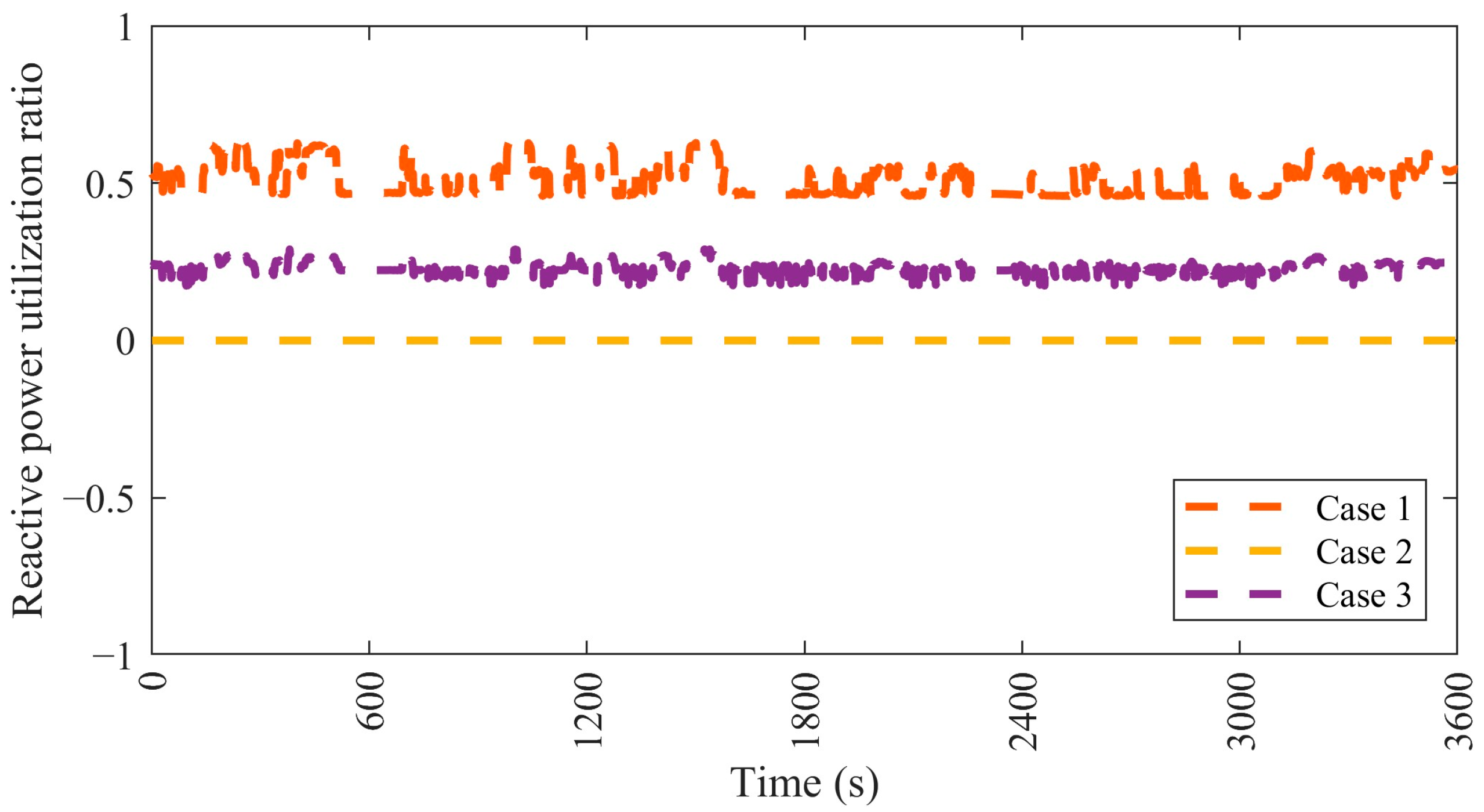
3.1. Reactive Power Utilization Ratio ()
3.2. Objective Function
- is the per unit voltage at DG node ;
- is the per unit voltage at non-DG node ;
- is the weight associated with voltage deviation minimization at DG nodes;
- is the weight associated with voltage deviation minimization at non-DG nodes;
- is the weight associated with minimizing the generation/consumption level of the reactive power;
- is the total number of DGs;
- is the total number of non-DG nodes.
3.3. Inputs and Outputs for the ANN
3.4. Communication Topology
3.5. Gradient Components
3.6. Gradient Gain
3.7. Updating Reactive Power Utilization Ratio Based on Consensus Algorithm
4. Results and Discussions
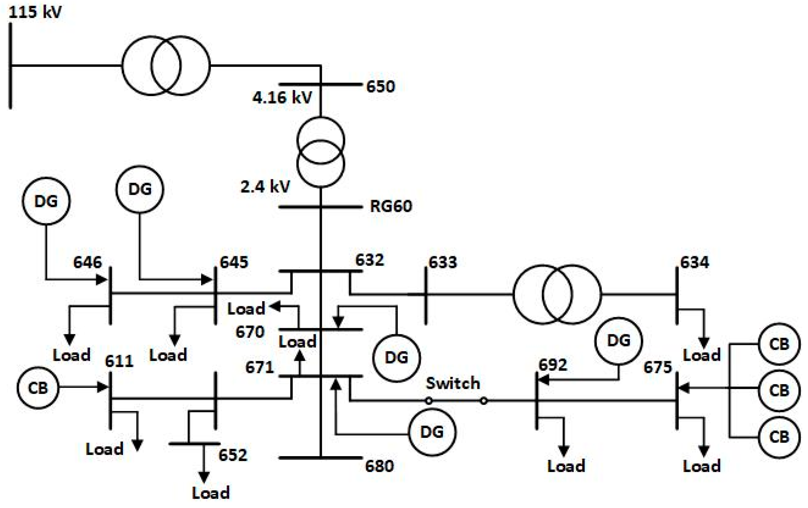
4.1. Power Distribution Network
4.2. Inputs and Outputs for the Neural Networks for the Modified IEEE 13-Bus System
4.3. Model-Free Cooperative Control
4.4. Comparative Analysis of Model-Based and Model-Free Cooperative Control
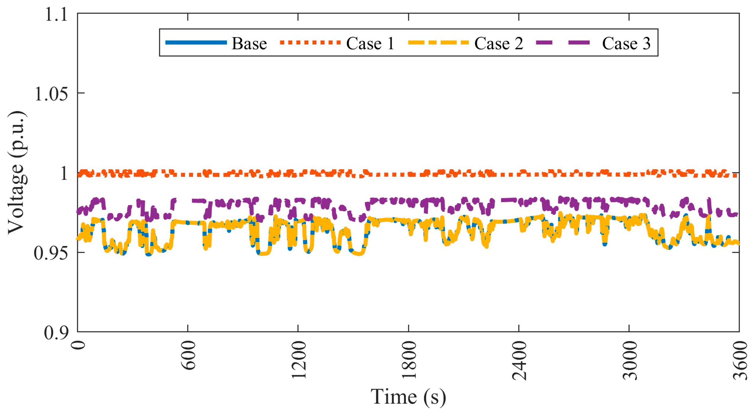
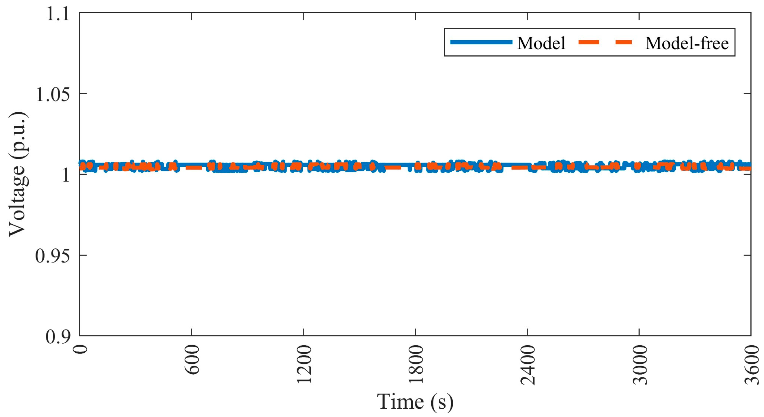
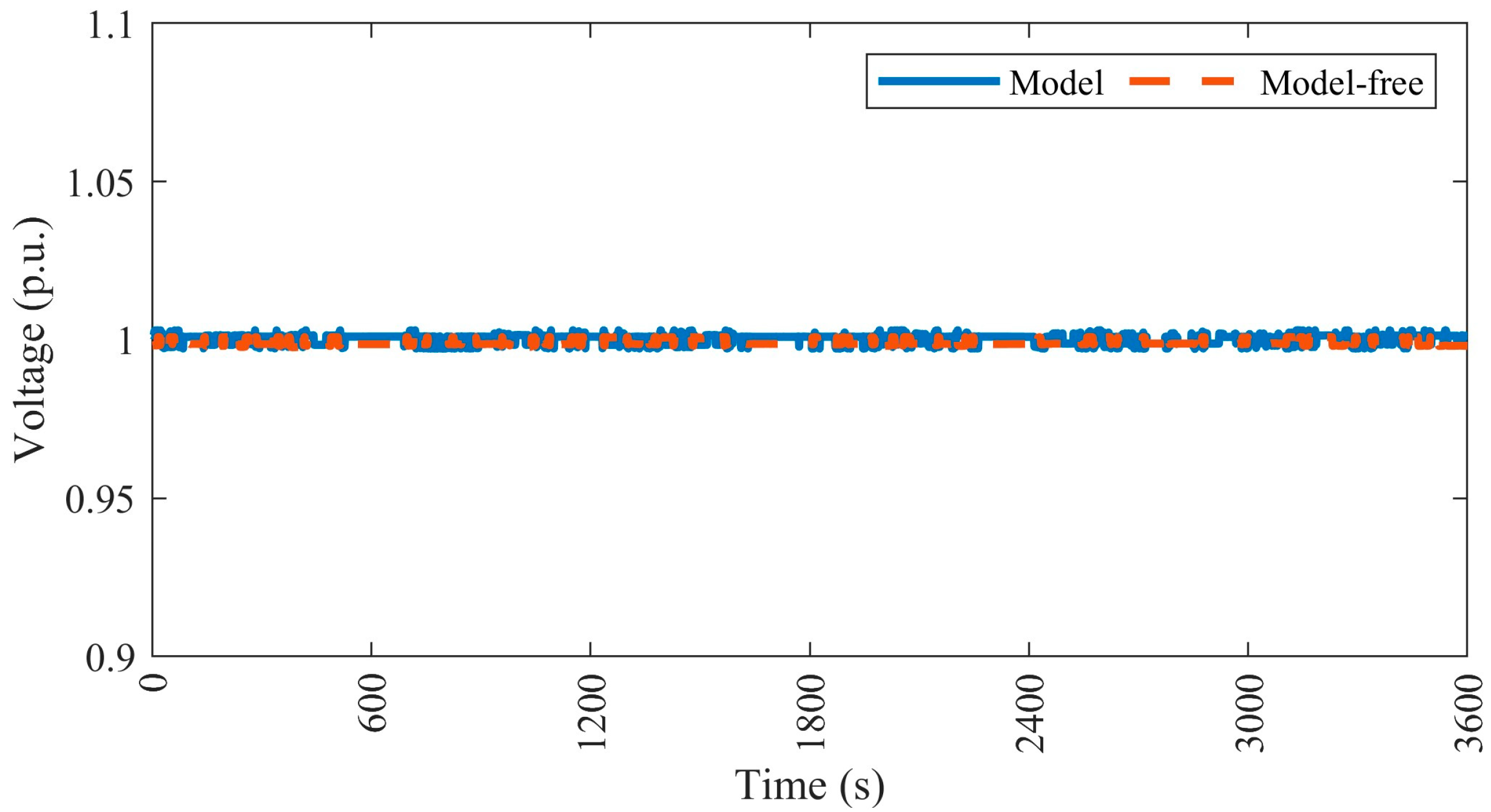
4.4.1. Case 1—Minimizing the Voltage Deviation
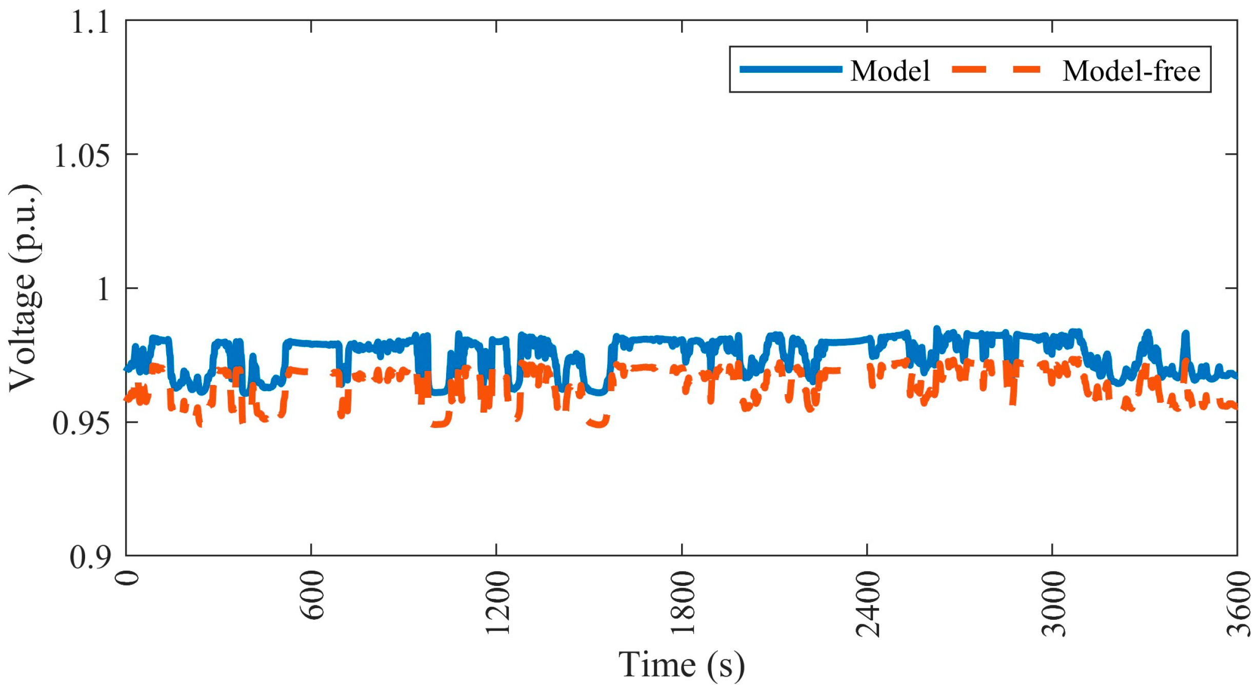
4.4.2. Case 2—Minimizing the Generation/Consumption of Reactive Power at DG Nodes
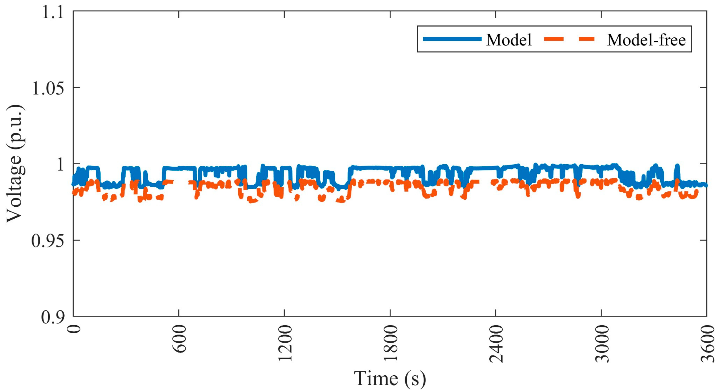
4.4.3. Case 3—Reducing Both the Reactive Power at DG Nodes and Voltage Deviation at DG and Non-DG Nodes
5. Conclusions
Author Contributions
Funding
Data Availability Statement
Conflicts of Interest
References
- Tunçel, S.; Gözel, T. The robust curve-fitting based method for coordinated voltage regulation with distributed generator and OLTC in distribution network. Alex. Eng. J. 2023, 75, 243–259. [Google Scholar] [CrossRef]
- Li, J.; Huo, Q.; Yin, J.; Liu, Q.; Sun, L.; Wei, T. Study on coordinated voltage regulation strategy of flexible on-load tap changer and distributed generator. Energy Rep. 2022, 8, 601–609. [Google Scholar] [CrossRef]
- Kabir, F.; Yu, N.; Gao, Y.; Wang, W. Deep reinforcement learning-based two-timescale Volt-VAR control with degradation-aware smart inverters in power distribution systems. Appl. Energy 2023, 335, 120629. [Google Scholar] [CrossRef]
- Hu, J.; Ye, C.; Ding, Y.; Tang, J.; Liu, S. A distributed MPC to exploit reactive power V2G for real-time voltage regulation in distribution networks. IEEE Trans. Smart Grid 2022, 13, 576–588. [Google Scholar] [CrossRef]
- Haghi, H.V.; Qu, Z. A Kernel-based predictive model of EV capacity for distributed voltage control and demand response. IEEE Trans. Smart Grid 2018, 9, 3180–3190. [Google Scholar] [CrossRef]
- Shang, C.; Fu, L.; Bao, X.; Xiao, H.; Xu, X.; Hu, Q. Dynamic joint optimization of power generation and voyage scheduling in ship power system based on deep reinforcement learning. Electr. Power Syst. Res. 2024, 229, 110165. [Google Scholar] [CrossRef]
- Xiong, M.; Yang, X.; Zhang, Y.; Wu, H.; Lin, Y.; Wang, G. Reactive power optimization in active distribution systems with soft open points based on deep reinforcement learning. Int. J. Electr. Power Energy Syst. 2024, 155, 109601. [Google Scholar] [CrossRef]
- Yadav, G.; Liao, Y.; Jewell, N.; Ionel, D.M. Cooperative control for mitigation of voltage fluctuations in power distribution systems. In Proceedings of the 2023 North American Power Symposium, NAPS 2023, Asheville, NC, USA, 15–17 October 2023. [Google Scholar] [CrossRef]
- Yadav, G.; Liao, Y.; Jewell, N.; Ionel, D.M. Dual-layer voltage and var control for power distribution systems. In Proceedings of the IEEE Power and Energy Society General Meeting, Seattle, WA, USA, 21–25 July 2024. [Google Scholar] [CrossRef]
- Maknouninejad, A.; Qu, Z. Realizing unified microgrid voltage profile and loss minimization: A cooperative distributed optimization and control approach. IEEE Trans. Smart Grid 2014, 5, 1621–1630. [Google Scholar] [CrossRef]
- Zhang, Y.; Wang, J.; Li, Z. Interval state estimation with uncertainty of distributed generation and line parameters in unbalanced distribution systems. IEEE Trans. Power Syst. 2020, 35, 762–772. [Google Scholar] [CrossRef]
- Cavus, M. Advancing power systems with renewable energy and intelligent technologies: A comprehensive review on grid transformation and integration. Electronics 2025, 14, 1159. [Google Scholar] [CrossRef]
- Qiu, W.; Yadav, A.; You, S.; Dong, J.; Kuruganti, T.; Liu, Y.; Yin, H. Neural networks-based inverter control: Modeling and adaptive optimization for smart distribution networks. IEEE Trans. Sustain. Energy 2024, 15, 1039–1049. [Google Scholar] [CrossRef]
- Guo, L.; Liu, Z.; Wang, Z.; Li, X.; Liu, Y.; Zhang, Y. Model-free optimal volt-var control of wind farm based on data-driven lift-dimension linear power flow. CSEE J. Power Energy Syst. 2025, 11, 91–101. [Google Scholar] [CrossRef]
- Li, S.; Wu, W.; Xu, J.; Dong, J.; Wang, F.; Yuan, Q. Zeroth-order feedback optimization for inverter-based volt-var control in wind farm. In Proceedings of the 2024 9th International Conference on Power and Renewable Energy, ICPRE 2024, Guangzhou, China, 20–23 September 2024; pp. 1384–1389. [Google Scholar] [CrossRef]
- Ren, H.; Jha, R.R.; Dubey, A.; Schulz, N.N. Extremum-seeking adaptive-droop for model-free and localized volt-var optimization. IEEE Trans. Power Syst. 2022, 37, 179–190. [Google Scholar] [CrossRef]
- Bagheri, P.; Xu, W. Model-free volt-var control based on measurement data analytics. IEEE Trans. Power Syst. 2019, 34, 1471–1482. [Google Scholar] [CrossRef]
- Hong, L.; Wu, M.; Wang, Y.; Shahidehpour, M.; Chen, Z.; Yan, Z. MADRL-based DSO-Customer coordinated bi-level volt/var optimization method for power distribution networks. IEEE Trans. Sustain. Energy 2024, 15, 1834–1846. [Google Scholar] [CrossRef]
- Zhang, Y.; Wang, X.; Wang, J.; Zhang, Y. Deep reinforcement learning based volt-var optimization in smart distribution systems. IEEE Trans. Smart Grid 2021, 12, 361–371. [Google Scholar] [CrossRef]
- Liu, H.; Wu, W.; Wang, Y. Bi-level off-policy reinforcement learning for two-timescale volt/var control in active distribution networks. IEEE Trans. Power Syst. 2023, 38, 385–395. [Google Scholar] [CrossRef]
- Glover, D.; Dubey, A. Centralized coordination of DER smart inverters using deep reinforcement learning. In Proceedings of the 2023 IEEE Industry Applications Society Annual Meeting, IAS 2023, Nashville, TN, USA, 29 October–2 November 2023. [Google Scholar] [CrossRef]
- Hua, D.; Peng, F.; Liu, S.; Lin, Q.; Fan, J.; Li, Q. Coordinated volt/var control in distribution networks considering demand response via safe deep reinforcement learning. Energies 2025, 18, 333. [Google Scholar] [CrossRef]
- Cao, D.; Zhao, J.; Hu, W.; Yu, N.; Ding, F.; Huang, Q.; Chen, Z. Deep reinforcement learning enabled physical-model-free two-timescale voltage control method for active distribution systems. IEEE Trans. Smart Grid 2022, 13, 149–165. [Google Scholar] [CrossRef]
- Li, S.; Wu, W.; Lin, Y. Robust data-driven and fully distributed volt/var control for active distribution networks with multiple virtual power plants. IEEE Trans. Smart Grid 2022, 13, 2627–2638. [Google Scholar] [CrossRef]
- Jeon, S.; Nguyen, H.T.; Choi, D.H. Safety-integrated online deep reinforcement learning for mobile energy storage system scheduling and volt/var control in power distribution networks. IEEE Access 2023, 11, 34440–34455. [Google Scholar] [CrossRef]
- Hernández-Gómez, O.M.; Vieira, J.P.A.; Tabora, J.M.; Sales e Silva, L.E. Mitigating voltage drop and excessive step-voltage regulator tap operation in distribution networks due to electric vehicle fast charging. Energies 2024, 17, 4378. [Google Scholar] [CrossRef]
- Nguyen, H.T.; Choi, D.H. Three-stage inverter-based peak shaving and volt-var control in active distribution networks using online safe deep reinforcement learning. IEEE Trans. Smart Grid 2022, 13, 3266–3277. [Google Scholar] [CrossRef]
- Wang, C.; Li, C.; Li, Y.; Liu, J.; Ling, F.; Liu, Q. A reinforcement learning based voltage regulation strategy for active distribution networks. In Proceedings of the 2023 2nd Asian Conference on Frontiers of Power and Energy, ACFPE 2023, Chengdu, China, 20–22 October 2023; pp. 433–437. [Google Scholar] [CrossRef]
- Zeng, Y.; Jiang, S.; Konstantinou, G.; Pou, J.; Zou, G.; Zhang, X. Multi-objective controller design for grid-following converters with easy transfer reinforcement learning. IEEE Trans. Power Electron. 2025, 40, 6566–6577. [Google Scholar] [CrossRef]
- Zeng, Y.; Xiao, Z.; Liu, Q.; Liang, G.; Rodriguez, E.; Zou, G.; Zhang, X.; Pou, J. Physics-informed deep transfer reinforcement learning method for the input-series output-parallel dual active bridge-based auxiliary power modules in electrical aircraft. IEEE Trans. Transp. Electrif. 2025, 11, 6629–6639. [Google Scholar] [CrossRef]
- Villarraga, D. AdaGrad—Cornell University Computational Optimization Open Textbook—Optimization Wiki. Available online: https://optimization.cbe.cornell.edu/index.php?title=AdaGrad (accessed on 17 November 2024).
- Ren, W.; Beard, R.W.; Atkins, E.M. Information consensus in multivehicle cooperative control. IEEE Xplore 2007, 27, 71–82. [Google Scholar]
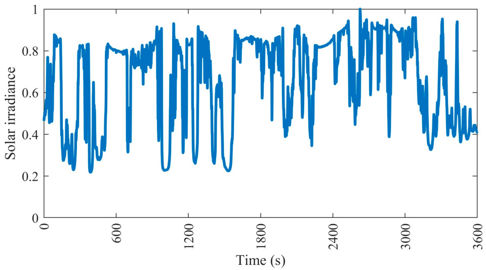
- Sengupta, M.; Andreas, A. Oahu Solar Measurement Grid (1-Year Archive): 1-Second Solar Irradiance; Oahu, Hawaii (Data). NREL Report No. DA-5500-56506. Available online: https://midcdmz.nrel.gov/apps/sitehome.pl?site=OAHUGRID (accessed on 18 May 2025).


| Phase | Buses | |
|---|---|---|
| DG Buses | Non-DG Buses | |
| A | 670, 671, 692 | 634, 652, 675 |
| B | 645, 670, 671 | 634, 646, 675 |
| C | 646, 670, 671 | 611, 634, 675, 692 |
| Case | Weights | Objective | ||
|---|---|---|---|---|
| 1 | 1 | 1 | 0 | Minimizes the voltage deviation |
| 2 | 0 | 0 | 1 | Minimizes the generation and consumption of reactive power |
| 3 | 1 | 1 | 0.1 | Reduce both voltage deviation and reactive power generation and consumption |
Disclaimer/Publisher’s Note: The statements, opinions and data contained in all publications are solely those of the individual author(s) and contributor(s) and not of MDPI and/or the editor(s). MDPI and/or the editor(s) disclaim responsibility for any injury to people or property resulting from any ideas, methods, instructions or products referred to in the content. |
© 2025 by the authors. Licensee MDPI, Basel, Switzerland. This article is an open access article distributed under the terms and conditions of the Creative Commons Attribution (CC BY) license (https://creativecommons.org/licenses/by/4.0/).
Share and Cite
Yadav, G.; Liao, Y.; Cramer, A.M. Model-Free Cooperative Control for Volt-Var Optimization in Power Distribution Systems. Energies 2025, 18, 4061. https://doi.org/10.3390/en18154061
Yadav G, Liao Y, Cramer AM. Model-Free Cooperative Control for Volt-Var Optimization in Power Distribution Systems. Energies. 2025; 18(15):4061. https://doi.org/10.3390/en18154061
Chicago/Turabian StyleYadav, Gaurav, Yuan Liao, and Aaron M. Cramer. 2025. "Model-Free Cooperative Control for Volt-Var Optimization in Power Distribution Systems" Energies 18, no. 15: 4061. https://doi.org/10.3390/en18154061
APA StyleYadav, G., Liao, Y., & Cramer, A. M. (2025). Model-Free Cooperative Control for Volt-Var Optimization in Power Distribution Systems. Energies, 18(15), 4061. https://doi.org/10.3390/en18154061