Electricity Load Forecasting Method Based on the GRA-FEDformer Algorithm

Abstract

In recent years, Transformer-based methods have shown full potential in power load forecasting problems. However, their computational cost is high, while it is difficult to capture the global characteristics of the time series. When the forecasting time length is long, the overall shift of the forecasting trend often occurs. Therefore, this paper proposes a gray relation analysis–frequency-enhanced decomposition transformer (GRA-FEDformer) method for forecasting power loads in power systems. Firstly, considering the impact of different weather factors on power loads, the correlation between various factors and power loads was analyzed using the GRA method to screen out the high-correlation factors as model inputs. Secondly, a frequency decomposition method for long short-time-scale components was utilized. Its combination with the transformer-based model can give the deep learning model an ability to simultaneously capture the fluctuating behavior of the short time scale and the overall trend of changes in the long time scale in power loads. The experimental results show that the proposed method had better forecasting performance than the other methods for a one-year dataset in a region of Morocco. In particular, the advantages of the proposed method were more obvious in the forecasting task with a longer forecasting length.

1. Introduction

With the booming social and economic development, and the continuous rise of power demand, accurately forecasting power loads has become a central challenge in the management and operation of modern power systems [1,2]. Power load forecasting is pivotal for the strategic planning, efficient dispatch and market operation of power systems. To date, numerous studies have employed statistical learning or machine learning techniques to perform power load forecasting, with significant results [3,4,5,6]. However, when faced with the complex task of load data forecasting, long-term dependencies are often embedded between historical observations and future forecasting results, which is a difficult challenge to be effectively modeled by traditional methods.

Fortunately, with the continuous development of deep learning technology, deep learning models based on recurrent neural network (RNN) architecture provide new ideas to solve this challenge. In particular, variants such as Long Short-Term Memory Networks (LSTMs) and Gated Recurrent Units (GRUs) have demonstrated an excellent ability to capture such long-term dependencies. These models shine in load data prediction tasks by introducing special gating mechanisms that can effectively remember historical information and forget useless information [7,8,9]. Nevertheless, these methods rely on saturated activation functions such as sigmoid or tanh. The derivatives of these activation functions converge to zero when the input values are large or small, which leads to the disappearance of the gradient between layers or the explosion phenomenon is still more prominent [10].

The Transformer algorithm greatly improves the parallel efficiency of computation through the clever introduction of the self-attention mechanism, and demonstrates an excellent ability in capturing long-term dependencies by virtue of its positional encoding mechanism [11,12,13]. This innovative feature has led to the emergence of numerous Transformer-based power load forecasting studies [14,15,16]. Ref. [14] proposed a prediction method based on Transformer and Complete Ensemble Empirical Mode Decomposition (CEEMDAN) to improve the forecasting accuracy. Ref. [16] proposed a Transformer-based load forecasting method that improves the problem of long-term memory loss by introducing an attention mechanism. Ref. [17] proposed an Autoformer-based load forecasting method, which accurately disassembles and captures complex patterns in a time series by adding an auto-correlation mechanism. Ref. [18] proposed a Deep Autoformer model. The MLP layer was combined on the framework of Autoformer to achieve more efficient depth information extraction.

Although Transformer-based methods have made significant progress in the field of time series forecasting, demonstrating strong modeling capabilities and adaptability, they still face the challenge of struggling to adequately capture the overall characteristics or distribution of the time series in some specific scenarios [19]. This problem is particularly prominent in the task of forecasting long time series, in which there is often a large difference between the trend of the predicted values and the true values over long time scales. This is mainly attributed to by a property of the Transformer model when dealing with time series data: the prediction for each time step is performed independently [20,21,22,23,24]. A comparison of various load forecasting methods is shown in

Table 1. Comparison of load forecasting methods.

Ref.	Year	Embedding	Adaptability to Long Time Series Forecasting Tasks	Adaptability to Short Time Series Forecasting Tasks
[11]	2017	Transformer	Non-adaptation	Adaptation
[14]	2023	CEEMDAN+Transformer	Non-adaptation	Adaptation
[15]	2023	GCN+ Transformer	Non-adaptation	Adaptation
[16]	2022	Multiple-Decoder Transformer	Non-adaptation	Adaptation
[17]	2024	CDConv+Autoformer	Non-adaptation	Adaptation
[18]	2022	MLP+Autoformer	Non-adaptation	Adaptation
[21]	2022	Informer	Non-adaptation	Adaptation
Proposed	-	GRA+FEDformer	Adaptation	Adaptation

.

In order to solve these problems, a gray relation analysis–frequency-enhanced decomposition transformer (GRA-FEDformer) method is proposed in this paper for solving the long time series prediction problem in load forecasting. Firstly, the mathematical and statistical method were as follows: GRA was utilized in analyzing the correlation between various collection variables and power loads, and filtering the main influencing factors. The embedding of GRA can enhance the learning efficiency of the predictive model and improve the overfitting problem. Secondly, the FEDformer algorithm was utilized. It can decompose a variety of collection variables in the frequency domain based on the fast Fourier transform (FFT) technique. And the features associated with power load trends were extracted through a stochastic screening strategy. On this basis, the processed frequency domain features were combined with Transfomer in order to capture the global attributes of the time series from an overall perspective. The main contributions of this paper are as follows:

(1)

A GRA-FEDformer method based on the mathematical–statistical method: GRA and a mixture of experts decomposition block is proposed, which can decompose the long time scale component and the short time scale component, and process them individually to better learn the characteristics of the variation in power load.

(2)

A frequency enhancement block based on FFT was utilized, and this module replaced the self-attention mechanism. The time series signals can be transformed into the frequency domain and important features of the time series can be captured from a global perspective.

(3)

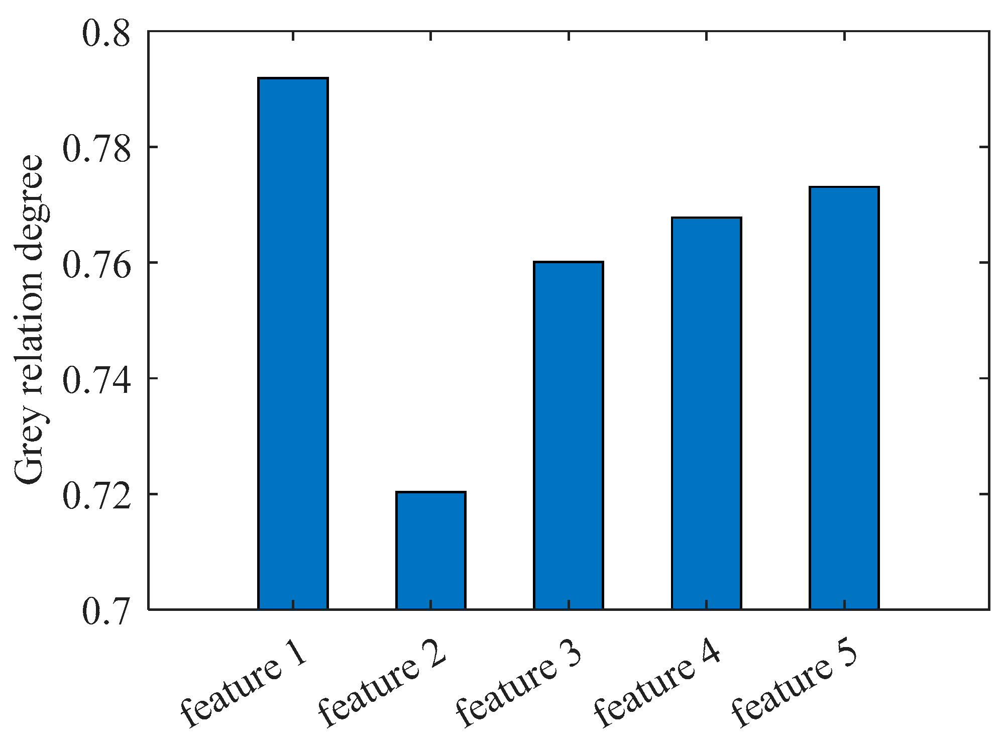
The GRA was applied to the prediction of power loads, which can effectively screen the sampled variables with high information entropy values.

In Section 2, the proposed GRA-FEDformer model is presented, in which the overall framework of the model and the way of constructing each sub-module are introduced, respectively; in Section 3, the power load forecasting method based on the GRA-FEDformer is presented; and in Section 4, the experimental results are demonstrated. In Section 5, the conclusion is given.

2. GRA-FEDformer Model

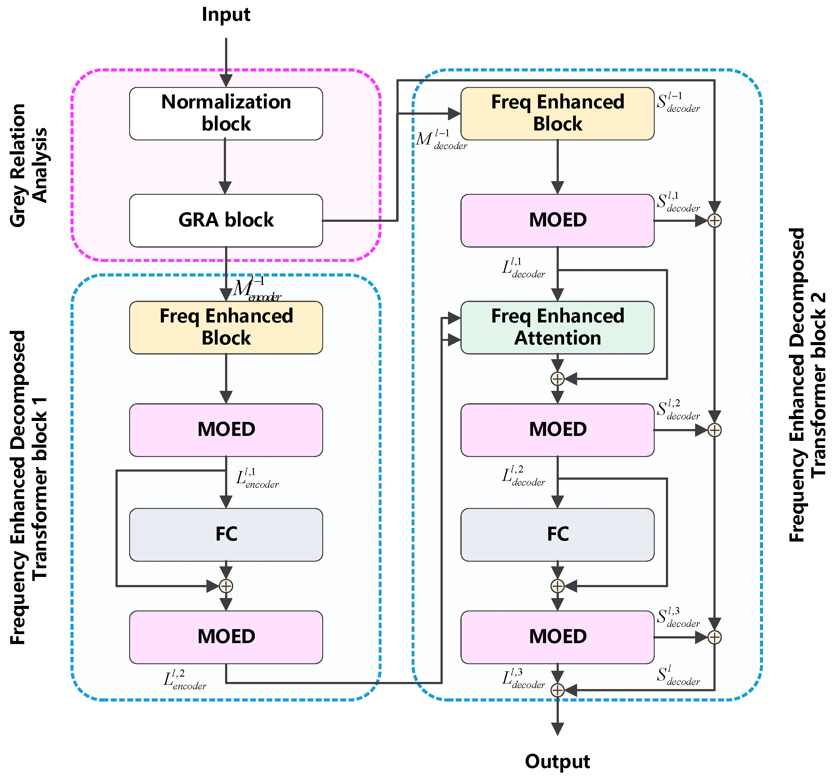
2.1. Model Framework

In this section, the structure of GRA-FEDformer is shown in Figure 1. It is mainly divided into two modules: (1) grey relation analysis block (GRA), which is mainly used to analyze the correlation degree between multiple sampled variables and predicted variables, and eliminate the variables with lower correlation degree and extract the variables with higher correlation degree. This module can improve the learning efficiency of the whole model. In the (2) FEDformer module, periodic patterns of multiple time scales are processed and captured in the frequency domain, which helps improve the accuracy of longer time series prediction. There are four main sub-modules in this module: frequency enhancement block (FEB), frequency enhancement attention (FEA), full connection network (FC), and mixture of experts decomposition block (MOED). Among them, the FEB and FEA can learn and reinforce effective features in the frequency domain; the MOED can extract and decompose periodic patterns in different time scales.

2.2. Grey Relation Analysis

The GRA module can determine the degree of similarity of trends based on the trends between the variables. Therefore, in this model, the role of this module was to analyze the degree of correlation between the variables so as to extract the variables with a higher correlation as the input of the next module. There are many types of data in the power system that are correlated with power loads; therefore, the data with a higher correlation need to be selected by GRA to enhance the learning efficiency of the deep learning algorithm and improve the overfitting problem. The specific steps of GRA are as follows.

Suppose that the sample data contain a time series of n variables, and the number of sampling points for each time series is d. Then, the sample features can be expressed as X₁(t), X₂(t), …, X_n(t). X_n(t) is a column vector denoted as [x_n(1), x_n(2), …, x_n(d)]. Then, due to the different amplitude ranges and units of each time series, it needs to be normalized with the following formula:

$$x_i(t)={\displaystyle \frac{x_i(t)-x_{i,\min }}{x_{i,\max }-x_{i,\min }}}$$

(1)

where x_i,min denotes the minimum value of the i-th time series; and x_i,max denotes the maximum value of the i-th time series.

Then, the grey correlation coefficients are calculated as follows:

$$\begin{array}{cc}{\zeta }_i(t)={\displaystyle \frac{\underset{i,t}{\min } \Delta x_i (t)+\rho \underset{i,t}{\max } \Delta x_i (t)}{\Delta x_i (t)-\rho \underset{i,t}{\max } \Delta x_i (t)}},& \Delta x_i (t)=\left|x_i (t)-x_0 (t)\right|\end{array}$$

(2)

where Δx_i(t) denotes the absolute difference between the i-th time series and the reference time series; and $\rho$ denotes the resolution coefficient, which is 0.5.

Finally, the grey correlation degrees are calculated as follows:

$$r_i={\displaystyle \frac{{\displaystyle \sum _{t=1}^d{\zeta }_i(d)}}{d}}$$

(3)

where r_i denotes the grey correlation degree of the i-th state variables and the reference state variables. The larger this value, the higher the correlation between the above two.

With the processing of the GRA module, we can obtain more compact and denser feature vectors X₁′ (t), X₂′ (t), …, X_m′ (t), where the length of each time series is constant.

2.3. FEDformer

This module has two main components, including the encoder and decoder. The specific structure of each of the two components will be described below.

The encoder adopts a multilayer structure as $M_{encoder}^l=Encoder\left(M_{encoder}^{l-1}\right)$, where $l\in \left\{1,\dots ,N\right\}$ denotes the output of l-th encoder layer. The input to the encoder is a historical time series $M_{encoder}^0\in {ℝ}^{I\times D}$. The expression for the encoder is shown below:

$$L_{encoder}^{l,1}=MOED(FEB(M_{encoder}^{l-1})+M_{encoder}^{l-1})$$

(4)

$$L_{encoder}^{l,2}=MOED(FF(L_{encoder}^{l,1})+L_{encoder}^{l,1})$$

(5)

where $L_{encoder}^{l,1}$ and $L_{encoder}^{l,2}$ denote the long period components of the output of the 1st or 2nd MOED module of the l-th encoding layer, respectively, and $L_{encoder}^{l,2}=M_{encoder}^l$.

The decoder also adopts a multilayer structure as $M_{decoder}^l,S_{decoder}^l=Decoder\left(M_{decoder}^{l-1},S_{decoder}^{l-1}\right)$. The structural expression of the decoding layer is shown below:

$$L_{decoder}^{l,1},S_{decoder}^{l,1}=MOED(FEB(M_{decoder}^{l-1})+M_{decoder}^{l-1})$$

(6)

$$L_{decoder}^{l,2},S_{decoder}^{l,2}=MOED(FEA(L_{decoder}^{l,1},L_{encoder}^{l,2})+L_{decoder}^{l,1})$$

(7)

$$L_{decoder}^{l,3},S_{decoder}^{l,3}=MOED(FF(L_{decoder}^{l,2})+L_{decoder}^{l,2})$$

(8)

$$S_{decoder}^{l,4}=S_{decoder}^{l-1}+w^{l,1}{S}_{decoder}^{l,1}+w^{l,2}{S}_{decoder}^{l,2}+w^{l,3}{S}_{decoder}^{l,3}$$

(9)

$$\begin{array}{c}{M}_{decoder}^l=L_{decoder}^{l,3}, S_{decoder}^l=S_{decoder}^{l-1}+w^{l,1}{S}_{decoder}^{l,1}+w^{l,2}{S}_{decoder}^{l,2}+w^{l,3}{S}_{decoder}^{l,3}\end{array}$$

(10)

$$Output=M_{decoder}^l+S_{decoder}^l$$

(11)

where $L_{decoder}^{l,1},S_{decoder}^{l,1}$ denotes the long-period mode and short-period mode component output from the 1st MOED module in the l-th layer decoder, respectively. $w^{l,1}$ denotes the projection of the 1st MOED module in the l-th layer decoder. The output is the prediction result of the whole decoder or FEDfomer, which consists of the individual long-period mode components and short-period mode components extracted by the model.

2.4. Frequency Enhancement Block

In this module, the input features are first transformed in the time domain:

$$q=x\cdot w$$

(12)

where x denotes the input to the FEB module with dimensions N × D, w denotes the linear transformation matrix with dimensions D × D, and q denotes the transformed time domain features.

On this basis, the frequency domain form of q needs to be obtained. Here, the fast Fourier transform was utilized to obtain the frequency domain form Q = F(q) with dimensions N × D. Then, M modes are randomly selected among the N frequency domain modes with the following formula:

$$Q^{\prime }=Select(Q)=Select\left(F\left(q\right)\right)$$

(13)

where Q′ has dimensions M × D. Finally, the frequency domain data are filled and an inverse fast Fourier transform is applied to get the result, as follows:

$$\begin{array}{cc}FEB(x)=F^{-1}(P(Y^{\prime })),& Y^{\prime }=Q^{\prime }\odot R\end{array}$$

(14)

where F⁻¹ denotes the inverse fast Fourier transform function and P denotes the padding function, which expands the dimensions of Y′ to N × D, with expansion values of zero. R is a matrix of dimensions D × D × M, and $\odot$ is the production operator.

2.5. Frequency Enhancement Attention

The inputs to this module are similar to the inputs to the Transformer-based model, including queries, keys, and values. All three inputs, q, k, and v, have dimensions N × D. The fast Fourier transform was applied to each of the three inputs, and M randomly filtered patterns in the frequency domain were obtained:

$$\begin{array}{ccc}{Q}^{\prime }=S(F(q)),& K^{\prime }=S(F(k)),& V^{\prime }=S(F(v))\end{array}$$

(15)

where Q′, K′, and V′ represent the frequency domain forms of queries, keys and values, respectively, with dimensions M × D.

Subsequently, based on Transformer’s attention mechanism, the improved frequency domain attention mechanism expression is shown below:

$$Attention(Q^{\prime },K^{\prime },V^{\prime })=\tanh \left(Q^{\prime }\cdot {K^{\prime }}^T\right)\cdot V^{\prime }$$

(16)

where tanh denotes an activation function. Finally, the output of the attention mechanism in the frequency domain is padded and inverse-fast-Fourier-transformed, then the expression of FEA was obtained:

$$FEA(Q^{\prime },K^{\prime },V^{\prime })=F^{-1}(P(Attention(Q^{\prime },K^{\prime },V^{\prime })))$$

(17)

2.6. Mixture of Experts Decomposition Block

In real scenarios, the sampled data do not have a single, simple pattern, but exhibit a mixture of periodic patterns with multiple different time scales. This makes it difficult for traditional methods, i.e., using fixed-window average pooling, to effectively decompose and extract features of various time scales from the data. Therefore, to address this problem, the MOED module was utilized. The core idea of the module lies in its internal integration of a variety of averaging filters of different sizes, which are capable of capturing and extracting trend components at multiple levels and different granularities from the input complex signals. Further, MOED not only has powerful trend extraction capabilities, but also incorporates a set of highly flexible and data-driven weighting mechanisms. These weights are not pre-set, but dynamically adjusted according to the specific characteristics of the input data to ensure that the previously extracted trend components are accurately weighted and combined to produce a more accurate and comprehensive representation of the final trend. The specific form of MOED is as follows:

$$Trend(x)=\mathrm{Softmax}(W(x)\cdot AP(x))$$

(18)

where W(x) denotes the weights of various different time scale components, and AP(x) denotes a set of average pooling filters.

From a formal point of view, we can describe the working principle of MOED in the following way: given an input signal, MOED filters it using a set of predefined averaging filters of different sizes, generating a series of trend components; subsequently, through a process of assigning weights that are closely related to the data, these trend components are skillfully combined to form a synthesis of all the important trend information in the final trend output. This process not only enhances the model’s ability to adapt to complex data structures, but also significantly improves the accuracy and robustness of trend extraction.

2.7. Frequency Domain Representation of Time Series Variables

There exist several forms of representation of time series variables, of which the most common forms are time domain representation and frequency domain representation. The power load forecasting model in this paper transforms and processes the time series in the frequency domain. However, the frequency component screening method used in the model of this paper is different from other power load forecasting models based on frequency domain representation. In this paper, the method of random screening was utilized to obtain a compact representation of time series variables in the frequency domain.

For multiple time series, they were Fourier-transformed into a frequency domain vector. This vector contained the frequency components corresponding to each frequency. Although retaining all the frequency components ensures a high degree of accuracy in time series reconstruction, this can easily lead to the overfitting problem, which in turn deteriorates the prediction performance of deep learning algorithms. Therefore, in this paper, we utilize a random screening method to randomly select some frequency components from all the frequency components and set the unselected portion to zero. As the time series such as power load in power system and weather data have a causal relationship and correlation with each other, its corresponding frequency domain Fourier matrix has an obvious low-rank nature. According to the CUR decomposition theory proposed in Ref. [20], the new Fourier matrix constructed by random screening can represent the original Fourier matrix to a certain extent.

3. Power Load Forecasting Method Based on GRA-FEDformer

The application process of the proposed power load forecasting method is shown in Figure 2. The detailed steps involved are as follows:

Step 1: Data Preprocessing. Since there may be significant differences in the range of variations in values of different variables, such differences may lead to the problem of the gradient explosion or disappearance, thus affecting the training effect and performance of the model. Therefore, first, the time series in the sample need to be normalized. In this paper, the standard normalization method was used. Then, the previous 48 moments in the time series were taken as the features of the sample, and the posterior 24, 48, 96, and 144 moments in the time series are taken as the prediction labels. The sliding interval of the time window is set to 24 in order to ensure that the pattern of load changes in a day can be learned effectively.

Step 2: Variable Screening. The dataset generally contains not only power load, but also environmental factors, meteorological factors and so on. In order to improve the learning efficiency, the GRA algorithm was used here to analyze the correlation between various variables and power load. Based on whether the correlation is greater than a set threshold, it is decided which variables should be retained.

Step 3: Model Training. The main objective in this step was to minimize the error between the real and predicted values of the power consumption load. The appropriate model parameters and hyperparameters are set and the training is done using the processed dataset. The loss function utilized is the root mean square error (MSE) with the following expression:

$$MSE={\displaystyle \frac{1}{n}}{{\displaystyle {\sum }_{i=1}^n\left(y_i-{\widehat{y}}_i\right)}}^2$$

(19)

where y_i denotes the actual value, and ŷ_i denotes the predicted value.

Step 4: Model Application. In this stage, for a specific load customer, its load in the previous 48 moments is obtained and inputted into the GRA-FEDformer model, so as to predict the trend of load in the future period. In order to illustrate the prediction accuracy of this model, the MSE, mean absolute error (MAE), standard deviation (SD) and margin of error (MOE) of 95% confidence interval (CI) were used as evaluation metrics.

$$MAE={\displaystyle \frac{1}{n}}{\displaystyle {\sum }_{i=1}^n\left|y_i-{\widehat{y}}_i\right|}$$

(20)

$$SD=\sqrt{{\displaystyle \frac{1}{n}}{\displaystyle {\sum }_{i=1}^n{\left(y_i-{\widehat{y}}_i\right)}^2}}$$

(21)

$$MOE=\pm 1.96\times SD$$

(22)

4. Experimental Results

4.1. Dataset Description

The dataset was selected from the power load data of a region and five meteorological data containing temperature, humidity, wind speed, general diffusive flow and diffusive flow for a region in Morocco in 2017, where the data are hourly, that is, data are collected every hour. To better validate the performance of the proposed method, the length of the input features was set to 48 h, i.e., 2 days of data. The length of the predicted labels was set to 24, 48, 96, and 144 h. The sliding interval of the time window was 24 moments. The training set and test set were divided in the ratio of 8:2.

4.2. Validation of Model Performance

4.2.1. GRA-Based Feature Selection Method

The weather environment affects the consumption of power loads to a certain extent. For example, extreme temperature changes can increase the frequency and duration of customers’ use of air conditioners, electric blankets, and other devices, which, in turn, leads to a significant climb in power loads. Therefore, in this paper, many kinds of local weather data were selected as input data to support the task of power load forecasting. However, the excessive feature data will enhance the computational complexity of the model, and at the same time, it may not necessarily be beneficial to improve the accuracy of the power load forecasting task. Therefore, in order to weigh the computational efficiency and computational accuracy, the GRA method was used here to analyze the grey correlation between multiple weather data and power loads, and the specific results are shown in Figure 3. It can be seen that temperature had the highest correlation with power load and could reach 0.7919. This shows that temperature had the greatest impact on power loads among these weather factors. In addition to this, wind speed, general diffuse flows and diffuse flows had correlations with power loads of roughly 0.76~0.77, while humidity had a correlation with power loads of only 0.7203 Therefore, the data of humidity were eliminated, and the other four meteorological data and power loads were used as inputs for the next algorithm module.

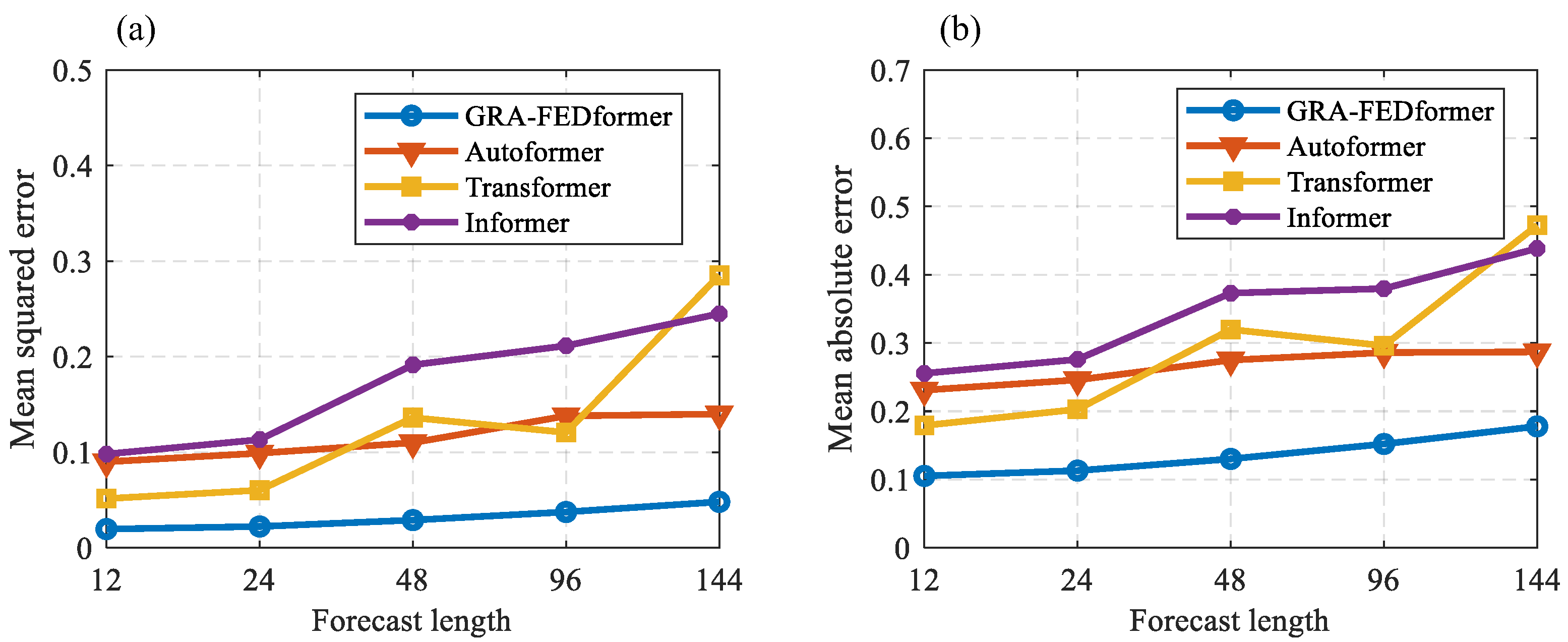
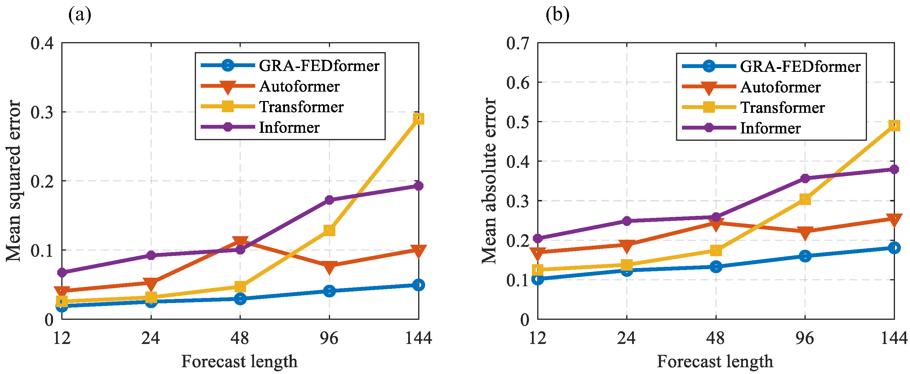
4.2.2. Analysis of the Results of Comparative Experiments

The experimental results for different forecast lengths are shown in

Table 2. Forecasting performance metrics (consideration of weather factors).

Forecast Length (Steps)	Proposed		Autoformer		Transformer		Informer
	MSE	MAE	MSE	MAE	MSE	MAE	MSE	MAE
12	0.019	0.105	0.090	0.231	0.051	0.179	0.098	0.255
24	0.022	0.113	0.099	0.246	0.060	0.202	0.113	0.276
48	0.029	0.130	0.110	0.275	0.136	0.319	0.191	0.373
96	0.037	0.152	0.138	0.286	0.120	0.296	0.211	0.379
144	0.048	0.177	0.140	0.287	0.285	0.472	0.244	0.438
	SD	MOE	SD	MOE	SD	MOE	SD	MOE
12	0.139	±0.273	0.272	±0.534	0.204	±0.400	0.225	±0.440
24	0.146	±0.287	0.306	±0.601	0.193	±0.378	0.255	±0.501
48	0.170	±0.334	0.247	±0.484	0.244	±0.477	0.258	±0.506
96	0.193	±0.379	0.362	±0.709	0.258	±0.506	0.299	±0.586
144	0.201	±0.392	0.272	±0.729	0.353	±0.692	0.281	±0.551

. It can be seen that the proposed method had the best forecast accuracy whether it was forecasting the load for the next half a day or forecasting the load for the next 6 days. Specifically, the MSE of the proposed method was 0.019 when the forecast length was 12. Compared to the Transformer, which had the highest accuracy among the compared methods, the MSE of the proposed method decreased by 0.031. The forecast error of the proposed method improved with the increase in forecast length. Each increase in forecast length improved the MSE of the proposed method by about 0.01. In contrast, in the comparison method, the improvement in forecast error was very large with the increase in forecast length. For example, the Transformer method had an MSE of 0.285 in the task of forecasting a length of 144, which is an improvement of 0.233 compared to that in the task of forecasting a length of 12, and was much larger than that of 0.028 corresponding to the proposed method. Thus, it can be shown that the proposed method had a significant advantage in the forecasting of long time series, which is attributed to the fact that it disassembles and reconstructs the frequency domain of the long time scale and short time scale components. In order to visualize the performance of the methods under different forecast lengths, Figure 4 shows the trend of the forecast performance with the forecast length. The blue line represents the proposed method, and it can be seen that its forecasting error was the smallest, and the forecasting error increased most gently with the increase in forecasting length.

In order to further validate the effectiveness and advantages of the proposed method in long time series forecasting tasks, and to reveal the trend of the performance of various methods with the forecast length, weather factors were not taken as model inputs and only power loads are taken as inputs. The forecast performance metrics of the methods at multiple forecast lengths (no consideration of weather factors) are shown in

Table 3. Forecasting performance metrics (no consideration of weather factors).

Forecast Length (Steps)	Proposed		Autoformer		Transformer		Informer
	MSE	MAE	MSE	MAE	MSE	MAE	MSE	MAE
12	0.019	0.101	0.040	0.169	0.025	0.125	0.067	0.204
24	0.025	0.123	0.052	0.188	0.031	0.137	0.092	0.248
48	0.029	0.132	0.113	0.244	0.047	0.173	0.100	0.258
96	0.040	0.159	0.077	0.222	0.128	0.303	0.172	0.356
144	0.049	0.180	0.100	0.255	0.289	0.490	0.192	0.379
	SD	MOE	SD	MOE	SD	MOE	SD	MOE
12	0.137	±0.269	0.190	±0.373	0.152	±0.299	0.201	±0.395
24	0.158	±0.309	0.218	±0.427	0.154	±0.303	0.221	±0.433
48	0.172	±0.336	0.336	±0.658	0.174	±0.341	0.256	±0.502
96	0.201	±0.394	0.269	±0.527	0.219	±0.430	0.251	±0.493
144	0.222	±0.435	0.298	±0.585	0.255	±0.500	0.257	±0.505

. Also the trend of the forecasting performance of each method is shown in Figure 5. It can be seen that the proposed method had the best forecasting performance at different forecasting lengths. In particular, the performance of the proposed method was significantly better than the comparison methods when the forecast length is long (length of 144).

In particular, observing the MSE curves of the proposed method and Transformer in Figure 5. It can be seen that the forecast error of the Transformer method shows an approximately exponential increase with the increase of the forecast length. This indicates that this method suffers from an overall shift in the task of forecasting long time series. And the proposed method solves this problem. It can be seen that the forecasting performance of the proposed method was excellent for all forecasting lengths. Meanwhile, the forecast error of the proposed method increased more slowly with the increase of forecast length. In summary, the proposed power load forecasting method had obvious advantages in the task of forecasting long time series.

4.2.3. Performance Validation for Frequency Mode Selection Strategies

In the process of transforming time series representations of power loads and other data from the time domain to the frequency domain, selecting an appropriate compact representation method in the frequency domain is crucial. This selection impacts the computational complexity of deep learning. Different compact representation methods in the frequency domain retain varying levels of useful information. Therefore, to balance computational complexity and the integrity of information retention, this paper adopts a random frequency component selection method.

To verify the performance of the proposed method, a comparison was made below between the random frequency component selection method and the mainstream lowest frequency component selection method. The forecasting performance indicators for both methods under different mode number (frequency components) are shown in Figure 6. Here, the input length of the model was set to 96, and the forecast length was also set to 96. It can be observed that the MSE and MAE corresponding to the random selection method were lower than those of the lowest frequency selection method in most cases. For example, when the mode number was set to 2, the MSE of the random selection method was 0.074, compared to 0.085 for the comparison method, resulting in a 12.43% reduction in error for the random selection method. When the mode number was 24, the MSE of the random selection method was 0.038, compared to 0.041 for the comparison method, indicating a 7.69% reduction in prediction error for the proposed method compared to the comparison method. In summary, under the premise of retaining the same number of frequency components and ensuring computational complexity, the random frequency component selection method retained more effective information related to power load changes compared to the mainstream low-frequency component selection method (which retains low-frequency components and discards high-frequency components). This enables deep learning models to capture more time series features, thereby more accurately forecasting power loads.

5. Conclusions

This paper proposes a power load forecasting method based on the Transformer, namely GRA-FEDformer. This method is characterized by its applicability to long time series forecasting tasks. The proposed methodology incorporates a mixture of experts decomposition block within the framework of the frequency-domain Transformer model. This module effectively dissected the time series into its long and short term components, allowing for the individual processing and extraction of the underlying features of power load variations. Consequently, the forecasting model was empowered to comprehensively capture both the dynamics occurring on short-time scales and the periodic patterns spanning long-time scales. The experimental results demonstrate that the proposed method exhibited superior performance in power load forecasting in comparison with other mainstream deep learning methods. The performance of MAE of the proposed method was improved by 41.34% and 62.50% in short time series (prediction length of 12) and long time series (prediction length of 144) prediction tasks, respectively. In addition, the performance degradation of the proposed method was minimized as the prediction length increases.

References

1. Wei, N.; Yin, C.; Yin, L.; Tan, J.; Liu, J.; Wang, S.; Qiao, W.; Zeng, F. Short-term load forecasting based on WM algorithm and transfer learning model. Appl. Energy 2024, 353, 122087. [Google Scholar] [CrossRef]
2. Wang, X.; Yao, Z.; Papaefthymiou, M. A real-time electrical load forecasting and unsupervised anomaly detection framework. Appl. Energy 2023, 330, 120279. [Google Scholar] [CrossRef]
3. Mohandes, M. Support vector machines for short-term electrical load forecasting. Int. J. Energy Res. 2002, 26, 335–345. [Google Scholar] [CrossRef]
4. Lee, C.M.; Ko, C.N. Short-term load forecasting using lifting scheme and ARIMA models. Expert Syst. Appl. 2011, 38, 5902–5911. [Google Scholar] [CrossRef]
5. Cui, Z.; Hu, W.; Zhang, G.; Huang, Q.; Chen, Z.; Blaabjerg, F. Knowledge-Informed Deep Learning Method for Multiple Oscillation Sources Localization. IEEE Trans. Power Syst. 2025, 40, 2811–2814. [Google Scholar] [CrossRef]
6. Bashir, T.; Haoyong, C.; Tahir, M.F.; Liquang, Z. Short term electricity load forecasting using hybrid prophet-LSTM model optimized by BPNN. Energy Rep. 2022, 8, 1678–1686. [Google Scholar] [CrossRef]
7. Lin, T.; Guo, T.; Aberer, K. Hybrid neural networks for learning the trend in time series. In Proceedings of the Twenty-Sixth International Joint Conference on Artificial Intelligence, Melbourne, Australia, 19–25 August 2017. [Google Scholar] [CrossRef]
8. Kong, W.; Dong, Z.Y.; Jia, Y.; Hill, D.J.; Xu, Y.; Zhang, Y. Short-term residential load forecasting based on LSTM recurrent neural network. IEEE Trans. Smart Grid 2017, 10, 841–851. [Google Scholar] [CrossRef]
9. Chiu, M.C.; Hsu, H.W.; Chen, K.S.; Wen, C.Y. A hybrid CNN-GRU based probabilistic model for load forecasting from individual household to commercial building. Energy Rep. 2023, 9, 94–105. [Google Scholar] [CrossRef]
10. Li, S.; Li, W.; Cook, C.; Zhu, C.; Gao, Y. Independently recurrent neural network (indrnn): Building a longer and deeper Indrnn. In Proceedings of the IEEE Conference on Computer Vision and Pattern Recognition, Salt Lake City, UT, USA, 18–22 June 2018. [Google Scholar] [CrossRef]
11. Vaswani, A.; Shazeer, N.; Parmar, N.; Uszkoreit, J.; Jones, L.; Gomez, A.N.; Kaiser, Ł.; Polosukhin, I. Attention is all you need. In Advances in Neural Information Processing Systems 30, Proceedings of the 31st Annual Conference on Neural Information Processing Systems (NIPS 2017), Long Beach, CA, USA, 4–9 December 2017; Curran Associates, Inc.: New York, NY, USA, 2018. [Google Scholar]
12. Khan, S.; Naseer, M.; Hayat, M.; Zamir, S.W.; Khan, F.S. Transformers in vision: A survey. ACM Comput. Surv. (CSUR) 2022, 54, 1–41. [Google Scholar] [CrossRef]
13. Wu, Y.; Liao, K.; Chen, J.; Wang, J.; Chen, D.Z.; Gao, H.; Wu, J. D-former: A u-shaped dilated transformer for 3d medical image segmentation. Neural Comput. Appl. 2023, 35, 1931–1944. [Google Scholar] [CrossRef]
14. Ran, P.; Dong, K.; Liu, X.; Wang, J. Short-term load forecasting based on CEEMDAN and Transformer. Electr. Power Syst. Res. 2023, 214, 108885. [Google Scholar] [CrossRef]
15. Qingyong, Z.; Jiahua, C.; Gang, X.; Shangyang, H.; Kunxiang, D. TransformGraph: A novel short-term electricity net load forecasting model. Energy Rep. 2023, 9, 2705–2717. [Google Scholar] [CrossRef]
16. Wang, C.; Wang, Y.; Ding, Z.; Zheng, T.; Hu, J.; Zhang, K. A transformer-based method of multienergy load forecasting in integrated energy system. IEEE Trans. Smart Grid 2022, 13, 2703–2714. [Google Scholar] [CrossRef]
17. Ming, L.; Chaoshan, S.; Yunfei, T.; Guihao, W.; Yonghang, L. An electricity load forecasting based on improved Autoformer. Comput. Technol. Dev. 2024, 35, 107–112. [Google Scholar] [CrossRef]
18. Jiang, Y.; Gao, T.; Dai, Y.; Si, R.; Hao, J.; Zhang, J.; Gao, D.W. Very short-term residential load forecasting based on deep-autoformer. Appl. Energy 2022, 328, 120120. [Google Scholar] [CrossRef]
19. Cleveland, R.B.; Cleveland, W.S.; McRae, J.E.; Terpenning, I. STL: A seasonal-trend decomposition. J. Off. Stat. 1990, 6, 3–73. [Google Scholar]
20. Wen, Q.; He, K.; Sun, L.; Zhang, Y.; Ke, M.; Xu, H. RobustPeriod: Robust time-frequency mining for multiple periodicity detection. In Proceedings of the 2021 International Conference on Management of Data, Virtual, 20–25 June 2021; Association for Computing Machinery: New York, NY, USA, 2021. [Google Scholar] [CrossRef]
21. Gong, M.; Zhao, Y.; Sun, J.; Han, C.; Sun, G.; Yan, B. Load forecasting of district heating system based on Informer. Energy 2022, 253, 124179. [Google Scholar] [CrossRef]
22. Drineas, P.; Mahoney, M.W.; Muthukrishnan, S. Relative-error CUR matrix decompositions. SIAM J. Matrix Anal. Appl. 2008, 30, 844–881. [Google Scholar] [CrossRef]
23. Zhou, H. Informer: Beyond efficient transformer for long sequence time-series forecasting. In Proceedings of the AAAI Conference on Artificial Intelligence, Virtual, 2–9 February 2021; AAAI Press: Washington, DC, USA, 2025. [Google Scholar] [CrossRef]
24. Wu, H.; Xu, J.; Wang, J.; Long, M. Autoformer: Decomposition transformers with auto-correlation for long-term series forecasting. In Advances in Neural Information Processing Systems 34, Proceedings of the 35th Conference on Neural Information Processing Systems (NeurIPS 2021), Vancouver, BC, Canada, 6–14 December 2021; Curran Associates, Inc.: New York, NY, USA, 2021. [Google Scholar]
Figure 1. Framework of the proposed GRA-FEDformer model for forecasting electricity loads.
Energies 18 04057 g001
Figure 2. The application process of the proposed power load forecasting method.
Energies 18 04057 g002
Figure 3. Gray correlation value between various weather data and power loads. Features 1~5 represent temperature, humidity, wind speed, general diffusive flow and diffusive flow, respectively.
Energies 18 04057 g003
Figure 4. Trends in the performance metrics (consideration of weather factors), (a) MSE; (b) MAE.
Energies 18 04057 g004
Figure 5. Trends in the performance metrics (no consideration of weather factors), (a) MSE; (b) MAE.
Energies 18 04057 g005
Figure 6. Trends in the performance metrics of the frequency component selection methods for various mode numbers, (a) MSE; (b) MAE.
Energies 18 04057 g006