Multi-Dimensional Feature Perception Network for Open-Switch Fault Diagnosis in Grid-Connected PV Inverters

Abstract

Intelligent monitoring and fault diagnosis of PV grid-connected inverters are crucial for the operation and maintenance of PV power plants. However, due to the significant influence of weather conditions on the operating status of PV inverters, the accuracy of traditional fault diagnosis methods faces challenges. To address the issue of open-circuit faults in power switching devices, this paper proposes a multi-dimensional feature perception network. This network captures multi-scale fault features under complex operating conditions through a multi-dimensional dilated convolution feature enhancement module and extracts non-causal relationships under different conditions using convolutional feature fusion with a Transformer. Experimental results show that the proposed network achieves fault diagnosis accuracies of 97.3% and 96.55% on the inverter dataset and the generalization performance dataset, respectively.

1. Introduction

With the growing global demand for sustainable energy, photovoltaic (PV) power generation has become a key component of national energy policies [1]. As a critical component of the system, the PV grid-connected inverter is responsible for converting direct current (DC) into alternating current (AC), and its reliability directly affects overall system performance [2,3]. During operation, inverters may encounter various types of faults, particularly switching faults [4,5], which mainly include single-switch and multi-switch faults [6]. Switching faults are often caused by aging of power devices or overload, leading to unbalanced inverter output and reduced system efficiency. A single-switch fault refers to the failure of an individual power switch (such as an IGBT or MOSFET), resulting in output voltage distortion and current imbalance, whereas a multi-switch fault involves simultaneous issues with multiple switches, potentially causing more severe system instability. If these faults are not detected and addressed in time, they can reduce power generation efficiency and may damage equipment [7]. Therefore, establishing an effective switch fault diagnosis program is essential for the operation and maintenance of PV power plants.

Researchers have developed various methods to monitor the operational status of IGBTs in inverters, including model-based approaches and deep learning-based approaches. Model-based methods distinguish faults by extracting current or voltage characteristics during fault conditions. Refs. [8,9,10] proposed a rapid open-circuit fault diagnosis method for neutral-point clamped three-level three-phase inverters based on residual evaluation. A diagnostic observer was constructed to obtain three-phase current observations and calculate current residuals through an observation matrix, achieving accurate fault detection and localization. Ref. [11] introduced a fault diagnosis method based on carrier-stacked modulation technology, analyzing the output characteristic curves of H-bridge output voltage, load current, and drive signals. This method extended the fault range under LSPWM to dual-switch faults. Its diagnostic logic is easy to understand and does not require additional hardware circuits. Ref. [12] used a three-phase output current as the fault characteristic and proposed an open-circuit fault diagnosis method for ANPC three-level inverters based on a switching modulation strategy. The method first roughly determines the fault switch device using the current average value method, then switches the modulation strategy to achieve fast online diagnosis. However, these methods rely on prior knowledge and expert experience and often require intrusive techniques in engineering practice, which may reduce diagnostic performance in complex scenarios [13,14].

With the rapid development of artificial intelligence, deep learning has become a research hotspot in inverter switch fault diagnosis [15,16]. Ref. [17] proposed an open-circuit fault diagnosis method based on a convolutional neural network, which was applied to a three-phase two-level inverter and achieved high fault diagnosis accuracy. Refs. [18,19] introduced a fault diagnosis method based on energy spectral entropy and wavelet neural networks. It used the upper, middle, and lower bridge arm voltages of an ANPC three-level inverter as measurement signals and employed an adaptive moment estimation wavelet neural network to establish a fault dictionary, achieving high-precision fault diagnosis. Ref. [20] designed a Causal-Res fault diagnosis method based on multi-connotation causal analysis, which deeply explored the potential causal relationships among the three-phase output current signals of the inverter. By combining this with the feature learning capability of residual neural networks, the method classified fault feature vectors to achieve fault diagnosis.

To address the operational characteristics of PV grid-connected inverters under multiple weather-influenced conditions, this paper proposes a fault diagnosis network based on a multi-dimensional feature perception network. The proposed network effectively integrates a multi-dimensional feature fusion module and a multi-scale convolutional Transformer. First, the model combines the multi-dimensional feature fusion module to efficiently capture multi-scale information of the input fault features in both channel and spatial dimensions. Then, the fault features are passed through the multi-scale convolutional Transformer to capture non-causal relationships of similar faults across different operating conditions. The multi-dimensional feature perception network effectively combines the strengths of both modules, ensuring robustness and accuracy of fault diagnosis under various weather scenarios.

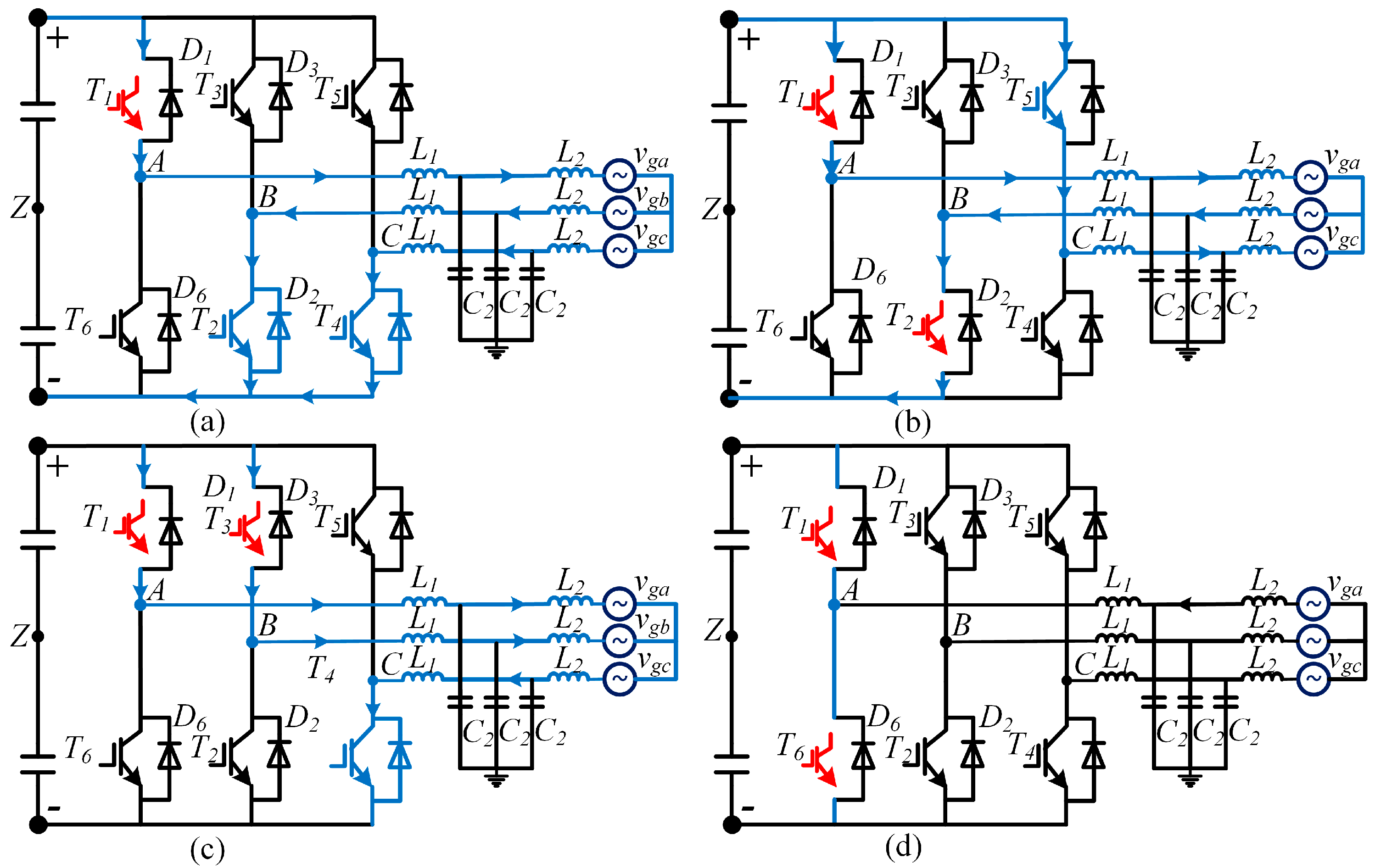
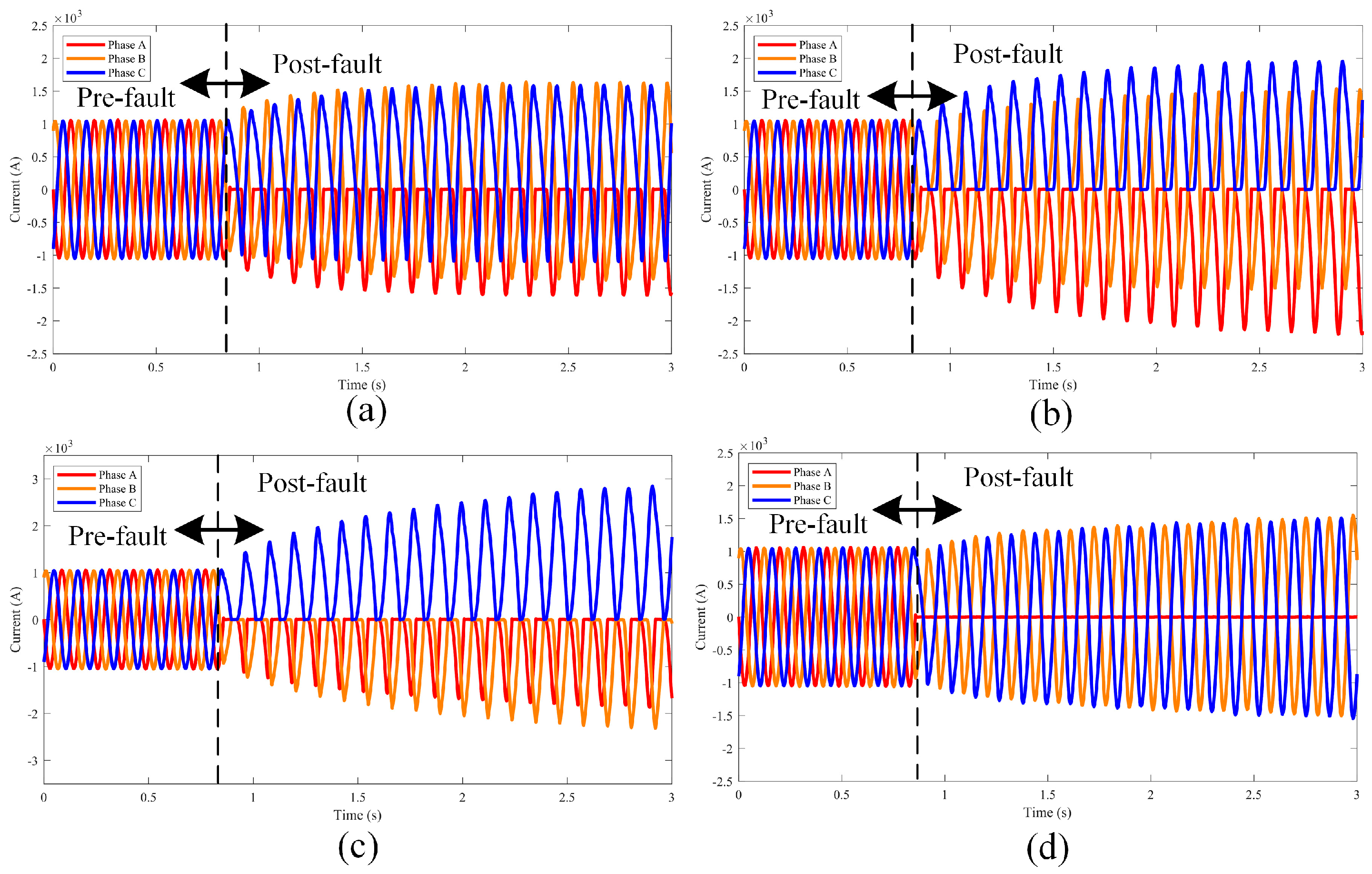
2. Open-Switch Fault Analysis of PV Grid-Connected Inverter

The structural diagram of the PV grid-connected inverter is shown in Figure 1. The specific electrical configuration includes a PV array, DC-DC boost converter, grid-connected inverter, LCL-type filter, and the upstream power grid. The main circuit and control parameters are selected based on the actual parameters of the PV power plant [21].

The PV array serves as the input power source in the PV grid-connected system. A simplified equivalent circuit model of the photovoltaic array consists of a current source in parallel with a diode. The equivalent mathematical model of the photovoltaic array can be expressed as [22]

$$I=I_{ph}-I_o\left[\exp \left({\displaystyle \frac{q\left(V+R_{s}I\right)}{nkT}}\right)-1\right]-{\displaystyle \frac{V+R_{s}I}{R_{sh}}}$$

(1)

where I_o is the diode saturation current, I_ph is the photocurrent, n is the ideality factor of the diode, k is the Boltzmann constant (1.38 × 10⁻²³ J·K⁻¹), q is the electron charge, R_s is the series resistance, and R_sh is the shunt resistance.

The function of the DC-DC boost converter circuit is to connect the PV array to the grid-connected inverter, matching the internal impedance of the PV panels with the external upstream power grid. The relationship between the DC voltage at the output side of the DC-DC boost converter and the output voltage of the photovoltaic array can be expressed as

$$U_{dc}=U_{pv}{\displaystyle \frac{1}{1-D}}$$

(2)

where D represents the duty cycle of the PWM signal, U_pv is the output voltage of the photovoltaic array, and U_dc is the DC-side voltage. In this paper, the incremental conductance method is used to adjust the duty cycle in order to maintain the output power of the PV array at its maximum power point.

Active power P and reactive power Q can be represented in the rotating coordinate system, where e_d and eq represent the d-axis and q-axis voltages, respectively, and id and i_q represent the currents on the d-axis and q-axis, respectively. The outer-loop power control can be expressed as

$$\left\{\begin{array}{l}{i}_{dref}={\displaystyle \frac{2}{3e_d}}\left(P-P_{ref}\right)\left(K_p+{\displaystyle \frac{K_i}{s}}\right)\hfill \\ i_{qref}=-{\displaystyle \frac{2}{3e_d}}\left(Q-Q_{ref}\right)\left(K_p+{\displaystyle \frac{K_i}{s}}\right)\hfill \end{array}\right.$$

(3)

where i_{d_ref} and i_{q_ref} are the reference values for id and iq, P_ref and Q_ref are the reference values for active and reactive power, and K_p and K_i are the proportional and integral gains, respectively. The feedforward decoupling control can be expressed as

$$\left\{\begin{array}{l}{e}_{dref}=e_d-\left(K_p+{\displaystyle \frac{K_i}{S}}\right)\left(i_{dref}-i_d\right)-\omega L{i}_q\hfill \\ e_{qref}=e_q-\left(K_p+{\displaystyle \frac{K_i}{S}}\right)\left(i_{qref}-i_q\right)+\omega L{i}_d\hfill \end{array}\right.$$

(4)

In this section, where applicable, authors are required to disclose details of how generative artificial intelligence (GenAI) has been used in this paper (e.g., to generate text, data, or graphics, or to assist in study design, data collection, analysis, or interpretation). The use of GenAI for superficial text editing (e.g., grammar, spelling, punctuation, and formatting) does not need to be declared.

The relationship between the input current of the LCL filter and the inverter output voltage U can be expressed as

$${\displaystyle \frac{I(s)}{U(s)}}={\displaystyle \frac{1}{L_1{L}_2{C}_2{s}^3+\left(L_1+L_2\right)s}}={\displaystyle \frac{1}{L_1{L}_{2}Cs\left(s^2+\frac{L_1+L_2}{L_1{L}_2{C}_2}\right)}}$$

(5)

where L₁ and L₂ represent the grid-side inductances and C₂ represents the grid-side capacitance. The specific system parameters of the PV grid-connected inverter are shown in

Table 1. Parameters of the PV grid-connected system.

Item	Parameters	Values
PV Array	Short-circuit current	isc = 1200 A
	Open-circuit voltage	voc = 640 V
	MPPT current	imppt = 1000 A
	MPPT voltage	vmppt = 502 V
DC-DC Boost Converter	Switch frequency	fsw = 10 kHz
	DC-side capacitance (C, C1)	(3 × 10−3 F, 4.7 × 10−2 F)
	DC-side inductor	L = 1 × 10−2 H
DC-AC Grid-Connected Inverter	Switch frequency	fsw = 10 kHz
	Current control loop (KPi, KIi)	(500, 1000)
	Power control loop (KPw, KIw)	(500, 1000)
	AC-side reference power	Pref = 500 kW
	AC-side reference active power	Qref = 0 kVA
LCL Filter	Grid-side inductor (L1, L2)	(1 × 10−3 H, 2.64 × 10−5 H)
	Grid-side capacitance	C2 = 1.5 × 10−7 F
Power Grid	Grid-side voltage	800 V

.

This paper considers a total of 21 different IGBT faults, including 6 single-switch faults and 15 dual-switch faults. These faults can be classified into four distinct categories: (1) single-switch faults, (2) dual-switch faults in different phases and different bridge arms, (3) dual-switch faults in different phases but the same bridge arm, (4) dual-switch faults in the same phase. The directions of the post-fault current under four specific types of faults are shown in Figure 2.

As shown in Figure 2a, under normal conditions, current flows through T₁ to the positive terminal. However, when a single-switch fault occurs in T₁, the forward current no longer flows through T₁ to the A-phase AC terminal, and the reverse current flows through the parallel diode D₁ of T₁ or T₆. Therefore, for a single-switch fault in T₁, a significant drop in A-phase current occurs only when the current is positive. This phenomenon can be clearly observed in Figure 3a.

For the dual-switch fault involving switches T₃ and T₅, corresponding fault currents appear during the positive half-cycles of phases B and C, respectively. Faults in switches T₆, T₄, and T₂ correspond to fault currents occurring during the negative half-cycles of phases A, B, and C, respectively.

In the case of open-circuit faults occurring in switches located in different phases and different bridge arms, such as T₁ and T₂, the forward current of phase A and the reverse current of phase B are unable to flow through T₁ and T₂, respectively. The current of phase B cannot pass through T₁ and T₂ and instead flows through the parallel diode D₁ or T₆, while the forward current of phase B flows through the parallel diode D₂ or T₃.

In the case of a dual-switch fault involving T₁ and T₂, a sharp drop in current occurs in both phases A and B only when the forward current of phase A is positive and the reverse current of phase B is negative.

For faults occurring in different phases but the same bridge arm, such as a fault in switches T₁ and T₃, the forward currents of phase A and phase B are unable to flow through T₁ and T₃, respectively. However, the reverse current of phase A will flow through the parallel diode D₁ or T₆, and the reverse current of phase B will flow through the parallel diode D₃ or T₂.

For faults occurring in the same phase, when switches T1 and T6 fail, both the forward and reverse currents in phase A cannot flow through T1 and T6. Figure 3b–d show the waveforms of three typical dual open-circuit faults. when the forward half-wave current of the corresponding phase drops sharply, the reverse current in the same phase also drops sharply.

3. Methods

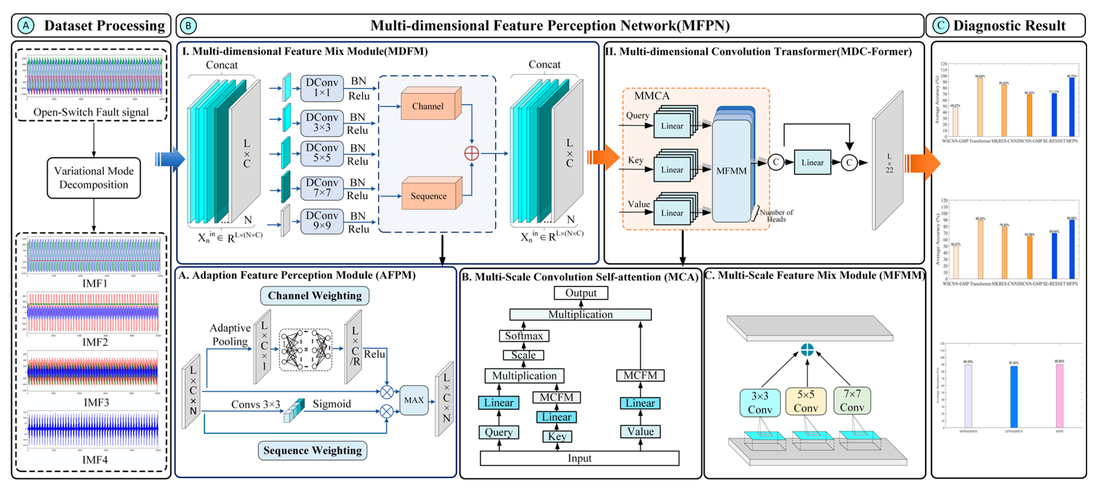
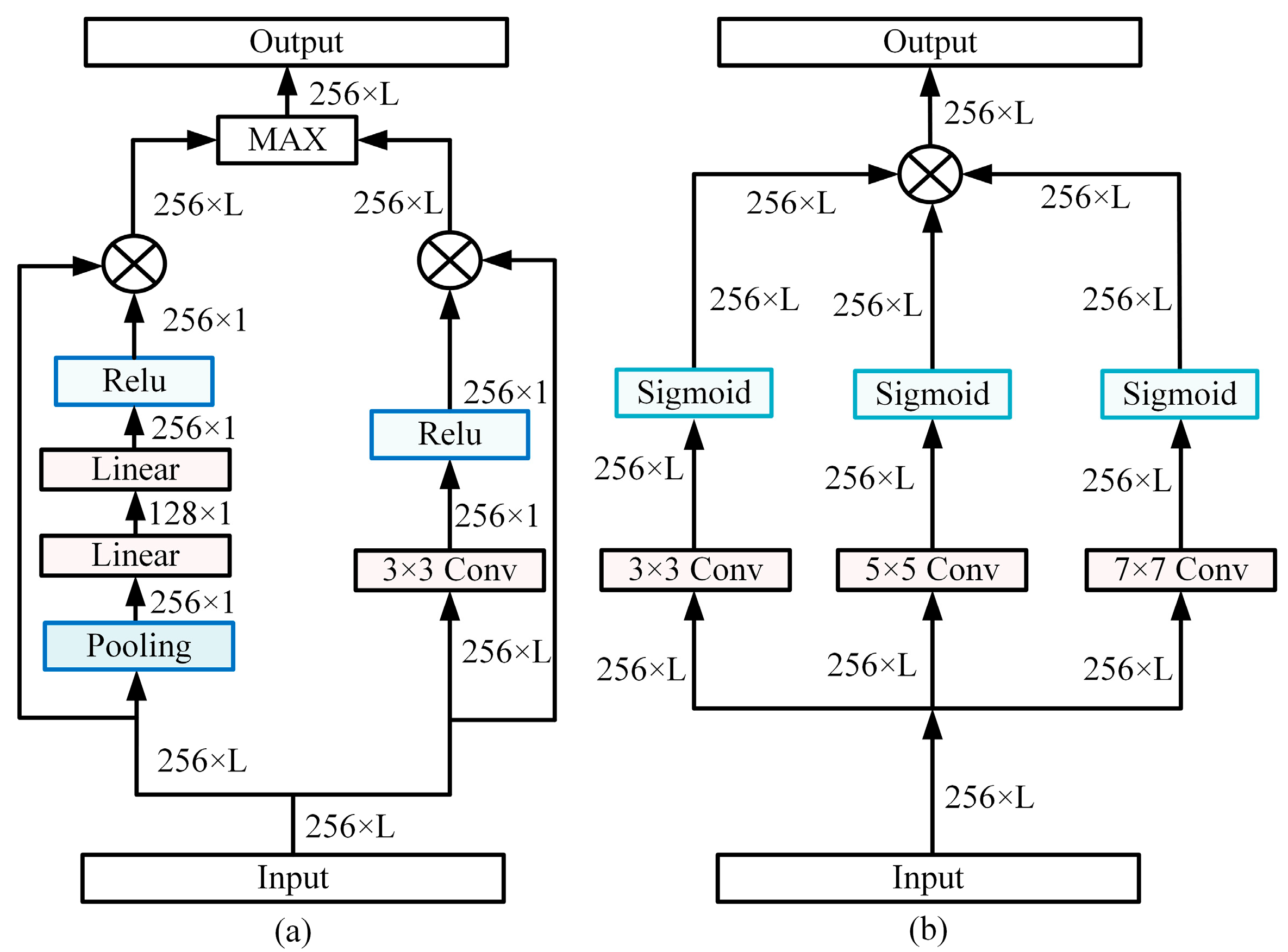
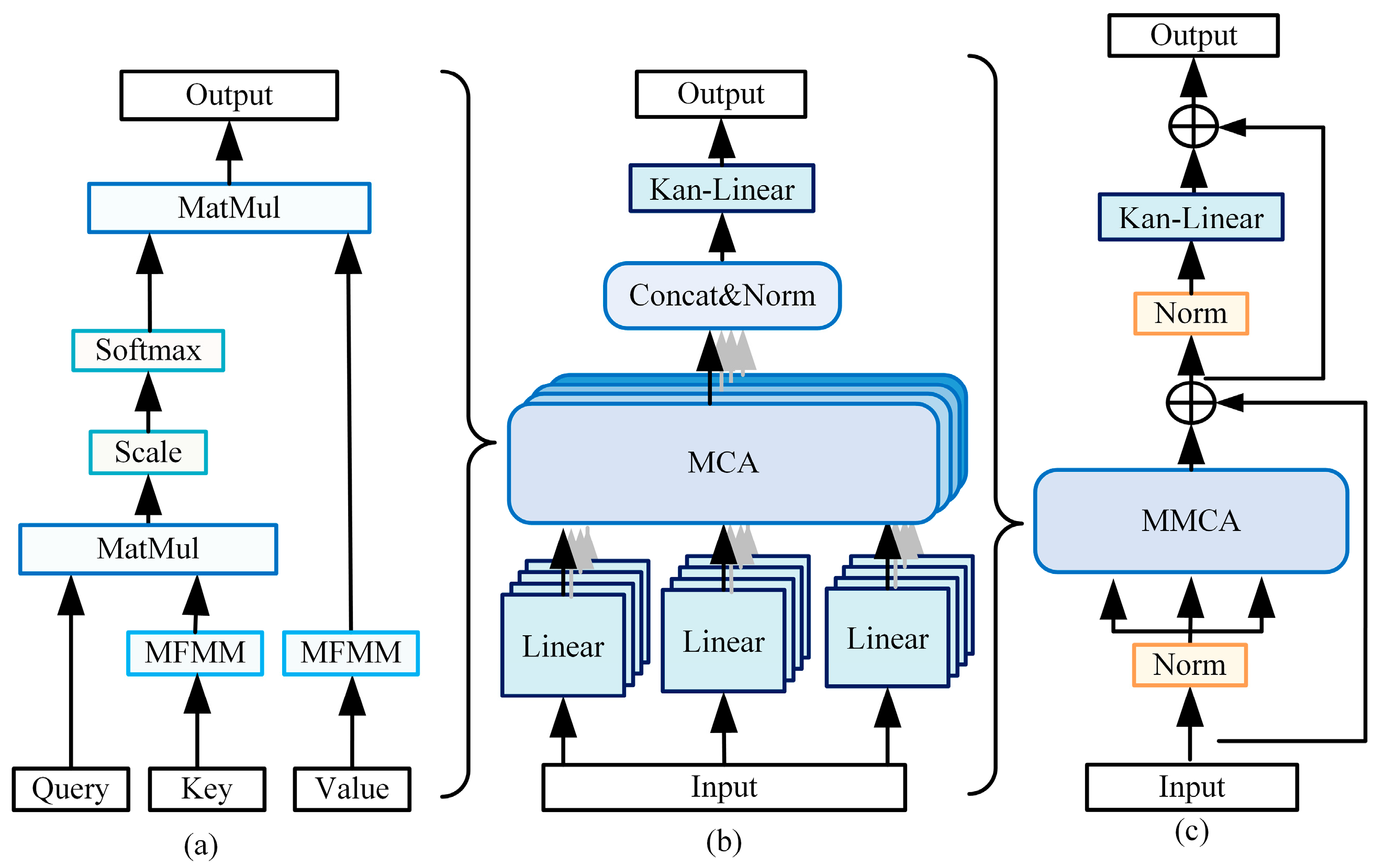
3.1. Fault Diagnosis Algorithm Based on Multi-Dimensional Feature Perception Network

Figure 4 shows the framework of the multi-dimensional feature perception network, which mainly consists of a multi-dimensional feature mix module and a multi-scale convolutional Transformer. The multi-dimensional feature fusion module is composed of multiple convolutional layers and an adaptive feature perception module. The multi-scale convolutional Transformer includes a multi-scale convolutional self-attention mechanism formed by a multi-scale convolutional fusion module, equipped with residual connections. This structure ensures that the multi-dimensional feature perception network maintains strong fault diagnosis robustness under various operating conditions.

The multi-dimensional feature mix module is designed to extract a comprehensive information weight matrix of fault features [23]. This module consists of multiple dilated convolutional layers and an adaptive feature perception module. The adaptive feature perception module calculates the channel weight matrix and sequence matrix of fault information to further compute integrated weighted features [24], aiming to fully capture global information of fault characteristics under various operating conditions of PV grid-connected inverters.

First, the fault signal is decomposed into four independent modes using Variational Mode Decomposition (VMD). VMD assumes that the signal is composed of intrinsic mode functions (IMFs) with specific center frequencies and limited bandwidths, enabling the decomposition of the signal into sub-signals. In electrical signals, fault features typically exhibit unique frequency characteristics [25]. Therefore, the VMD method is employed to analyze the output current signals of the inverter to distinguish between different fault patterns. VMD effectively extracts different modes from the signal, aiding in the identification and diagnosis of inverter fault types under varying operating conditions. The mathematical expression of VMD can be represented as

$${\widehat{u}}_k^{n+1}(\omega )={\displaystyle \frac{\widehat{f}(\omega )-{\displaystyle \sum _{i\ne k}}{\widehat{u}}_i(\omega )+\frac{\widehat{\lambda }(\omega )}{2}}{1+2\alpha {\left(\omega -{\omega }_k\right)}^2}}$$

(6)

$${\omega }_k^{n+1}={\displaystyle \frac{{\int }_0^{\mathit{\infty }}\omega {\left|{\widehat{u}}_k(\omega )\right|}^{2}d\omega }{{\int }_0^{\mathit{\infty }}{\left|{\widehat{u}}_k(\omega )\right|}^{2}d\omega }}$$

(7)

where $\widehat{u}$ represents the mode components in different modes and $\omega$ denotes the center frequencies of the different modes. After the original fault signal is decomposed through modal decomposition, each mode component is referred to as IMF_nⁱⁿ.

Next, the four modal components are used as input signals, and three 3 × 3 convolutional layers are applied for multi-level feature extraction.

To further expand the network’s receptive field and capture multi-scale information of fault features, dilated convolutions with different kernel sizes and dilation rates are applied on five separate branches to convolve the original input features. Then, the outputs of the five branches are summed to fully integrate the multi-scale information of the fault features. The system output X_in can be expressed as follows:

$$X^{in}={\displaystyle \mathbf{\prod }_{n=1,3,5,7,9}\mathrm{BN}\left(\sigma \left({\mathrm{DConv}}_{nxn}\left(IM{F}_n^{in}\right)\right)\right)}$$

(8)

where $\sigma$ represents the activation function.

The adaptive feature perception module, as shown in Figure 5a, first uses adaptive average pooling in the channel feature section to obtain the importance weight of each channel. Then, two fully connected layers are used to learn the importance weights of each channel. Finally, the channel weights are multiplied element-wise with the original fault features to achieve channel-wise weighting of the original fault features.

$$P_{channel}=\sigma \left(\mathrm{Linear}\left(\mathrm{AdaptivePooling}\left(X^{in}\right)\right)\right)$$

(9)

where P_channel represents the channel feature weights.

In the sequence feature section, the input feature X_in is passed through a single convolutional layer with a kernel size of 3 to capture the spatial weights of the fault features, followed by a Sigmoid activation function. The mathematical process of this operation can be expressed as

$$P_{sequence}=\sigma \left({\displaystyle \mathbf{\prod }_{n=3,5,7}\mathrm{BN}(\mathrm{ReLU}({\mathrm{Conv}}_{n\mathrm{x}n}\left(X^{in}\right)}\right)$$

(10)

where P_sequence represents the spatial feature weights.

To obtain a comprehensive representation of the fault features, the channel weight matrix and the spatial weight matrix are added element-wise to obtain the integrated feature weight D. The mathematical process of this operation can be expressed as

$$D=\sigma \left(P_{\mathrm{channel}}\oplus P_{\mathrm{sequence}}\right)$$

(11)

The mathematical process for calculating the output of the combined features can be expressed as

$$X^{out}=D\otimes X^{in}$$

(12)

In summary, the multi-dimensional feature mix module concatenates the output features of the multi-scale dilated convolutions along the channel dimension and adjusts the weights using both channel and spatial attention mechanisms. This not only enables the fusion of features from multiple perspectives but also integrates features from different dilated convolution layers with global features. In this way, the network can focus on local details while effectively capturing global information.

To ensure the robustness of the multi-dimensional feature perception network’s diagnostic performance in generalization testing scenarios, this paper proposes a multi-scale convolutional self-attention mechanism. This mechanism selects keys and values through a multi-scale convolutional fusion module to further capture non-causal relationships between similar faults under different operating conditions. The structure of the multi-scale convolutional mix module is shown in Figure 5b. It performs convolution operations on the original input fault features using three different convolution kernels with sizes 3, 5, and 7, respectively. The convolved fault features are then summed. The mathematical process of the above operation can be expressed as

$$y^{mix}={\displaystyle \mathrm{\prod }_{n=3,5,7}\sigma \left({\mathrm{Conv}}_{nxn}\left(x^{out}\right)\right)}$$

(13)

where y_mix represents the mixed feature output.

As shown in Figure 6a, self-attention is applied to the queries, keys, and values in the multi-head attention mechanism [26]. The mathematical process of this operation can be expressed as follows:

$$y_i^{out}=Softmax\left({\displaystyle \frac{Q_i{K}^T}{\sqrt{d_k}}}\right)V,\hspace{1em}1\le i\le L$$

(14)

For the edge information of fault features, the multi-head convolutional self-attention mechanism uses a padding strategy to maintain the sequence length.

As shown in Figure 6b, for a given input feature xout, a linear layer is applied to perform linear projection and obtain the corresponding queries, keys, and values [27]. Next, the input features are decomposed into different subspaces, and a multi-scale convolutional self-attention mechanism is performed in each head. The proposed multi-head convolutional self-attention mechanism can be described as follows:

$$y_i^{\mathrm{out}}=\mathrm{MHCA}\left(Q_i,K_i,V_i\right),\hspace{1em}1\le i\le T$$

(15)

$$y^{\mathrm{out}}=\mathrm{Linear}\left(\mathrm{Concat}\left[y_1^{\mathrm{out}},\dots ,y_n^{\mathrm{out}}\right]\right)$$

(16)

As shown in Figure 6c, to further enhance the model’s stability during training, residual connections are used as the output. In the classification stage, a single linear layer is used as the classifier. The overall structure of the MDC-former can be represented as follows:

$$Y^{out}=\mathrm{Linear}(\mathrm{Norm}(Y^{out}))+Y^{out}$$

(17)

Overall, compared to conventional Transformer architectures, the multi-scale convolutional Transformer possesses multi-scale linear representation capabilities and can capture non-causal relationships among the input fault features [28,29].

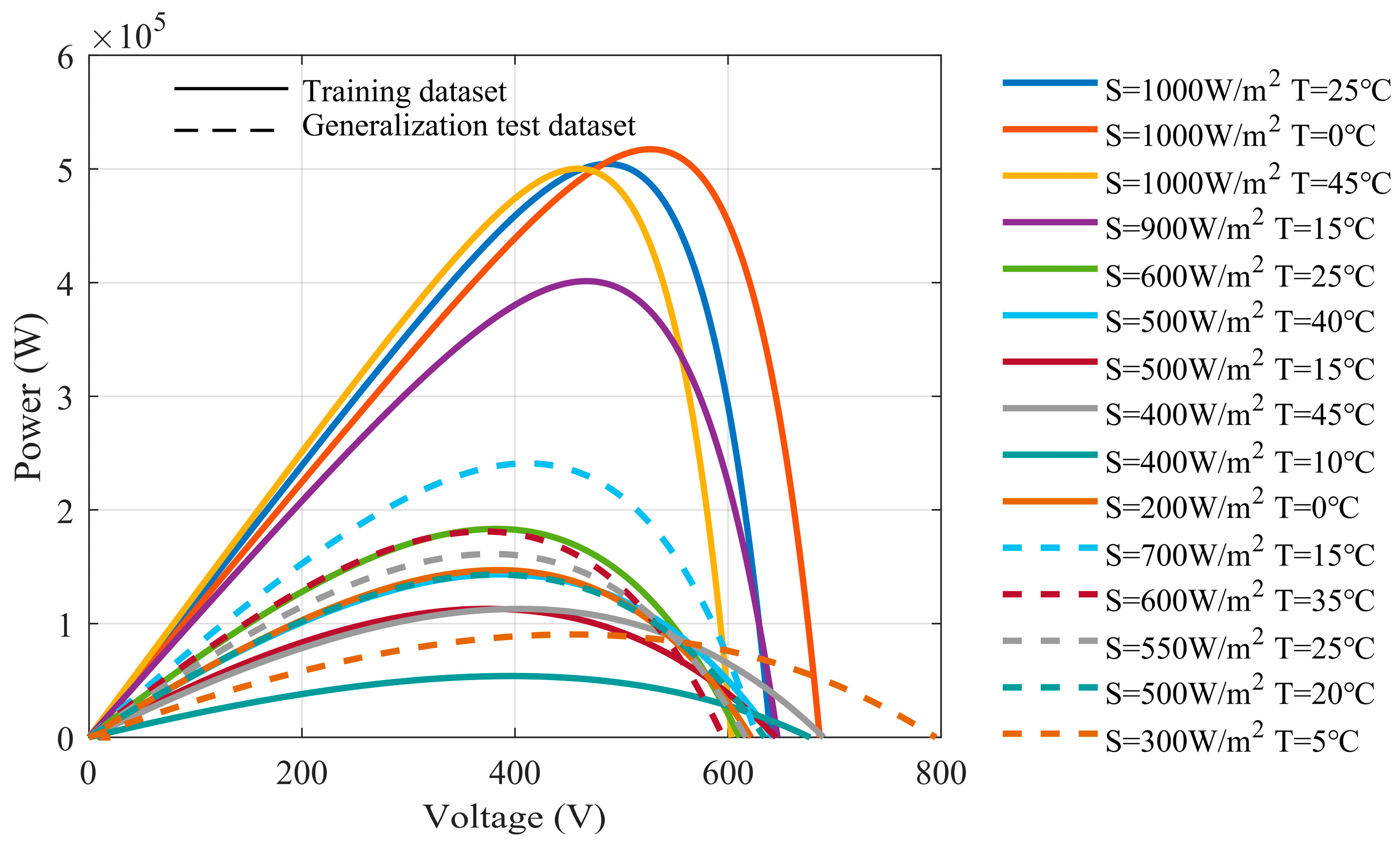
3.2. Hardware in the Loop Platform Dataset

To investigate the relevant scenarios of the high-power PV grid-connected system [30], HIL experiments were conducted. Figure 7 illustrates the HIL platform used for these experiments, consisting of a host computer, an FPGA-based real-time simulator (NI-PXIe-FPGA-7868R, National Instruments, Austin, TX, USA), an oscilloscope, and input/output boards. The host computer, equipped with StarSim software (version 1.0.1), configures the hardware settings, which are then transmitted to the NI-PXIe-FPGA-7868R.

FPGA is one of the core hardware components of the entire real-time simulation system and is particularly well-suited to simulating power electronic systems that require extremely high computational precision and real-time performance. The power electronic models running on the FPGA use very small simulation time steps (typically in the nanosecond to microsecond range), enabling precise simulation of high-frequency switching devices, complex circuit topologies, and fast dynamic behaviors.

The CPU is mainly responsible for running user-defined Control Blocks. Control Blocks can serve various functions, such as implementing control algorithms for closed-loop control or simulating complex physical processes.

In PV power systems, the StarSim HIL platform can simulate the output characteristics of PV arrays, MPPT control algorithms, and the operational behavior of inverters. During closed-loop control strategy testing, the inverter model running on the FPGA works in coordination with the PV array model on the CPU to simulate a realistic operating environment.

In summary, the simulation platform based on StarSim can effectively simulate the operation of PV inverters, including the control loops and the behavior of IGBTs. However, there is still a gap between the theory and hardware operation. Further narrowing this gap between hardware simulation and actual systems will be the focus of future research.

As shown in Figure 8, to closely approximate the actual operating conditions of a photovoltaic power plant, the solar irradiance S (W/m²) and temperature T (°C) inputs to the PV grid-connected system are adjusted, and operational data were collected under 15 different conditions. Each sample contains 2000 measurement points.

The real-time simulator handles the control loops of the DC-DC converter and the grid-connected inverter, generating pulse width modulation (PWM) signals accordingly. During signal acquisition, the sampling frequency was set to 20 kHz. Each class comprises 1800 samples, with 1080 used for training, 120 for testing, and 600 for evaluating generalization performance. The dataset contains 22 different fault labels, as shown in the

Table 2. Illustration of PV grid-connected inverter dataset.

Class	Illustration	Training Data	Test Data	Total Data
0	Healthy Status	1080	720	1800
1	T1 Failure	1080	720	1800
2	T2 Failure	1080	720	1800
3	T3 Failure	1080	720	1800
4	T4 Failure	1080	720	1800
5	T5 Failure	1080	720	1800
6	T6 Failure	1080	720	1800
7	T1&T6 Failure	1080	720	1800
8	T3&T4 Failure	1080	720	1800
9	T5&T2 Failure	1080	720	1800
10	T1&T4 Failure	1080	720	1800
11	T1&T2 Failure	1080	720	1800
12	T3&T6 Failure	1080	720	1800
13	T3&T2 Failure	1080	720	1800
14	T5&T6 Failure	1080	720	1800
15	T5&T4 Failure	1080	720	1800
16	T1&T3 Failure	1080	720	1800
17	T1&T5 Failure	1080	720	1800
18	T3&T5 Failure	1080	720	1800
19	T4&T2 Failure	1080	720	1800
20	T6&T4 Failure	1080	720	1800
21	T6&T2 Failure	1080	720	1800
0	Healthy Status	1080	720	1800

. including: (1) Single-switch faults (2) Dual-switch faults in the same bridge arm (3) Dual-switch faults across different bridge arms and phases (4) Dual-switch faults across different bridge arms but in the same phase.

4. Results and Discussion

4.1. Configuration Settings

All comparison experiments were conducted on a system equipped with a GTX 4070 GPU and an Intel I7-14700KF CPU. In the experiments, the batch size for all comparison algorithms was set to 64 and the learning rate was set to 0.0001. The training and testing datasets were obtained from HIL platform dataset. Additionally, the multi-dimensional feature perception network was evaluated against five different comparison algorithms:

(1)

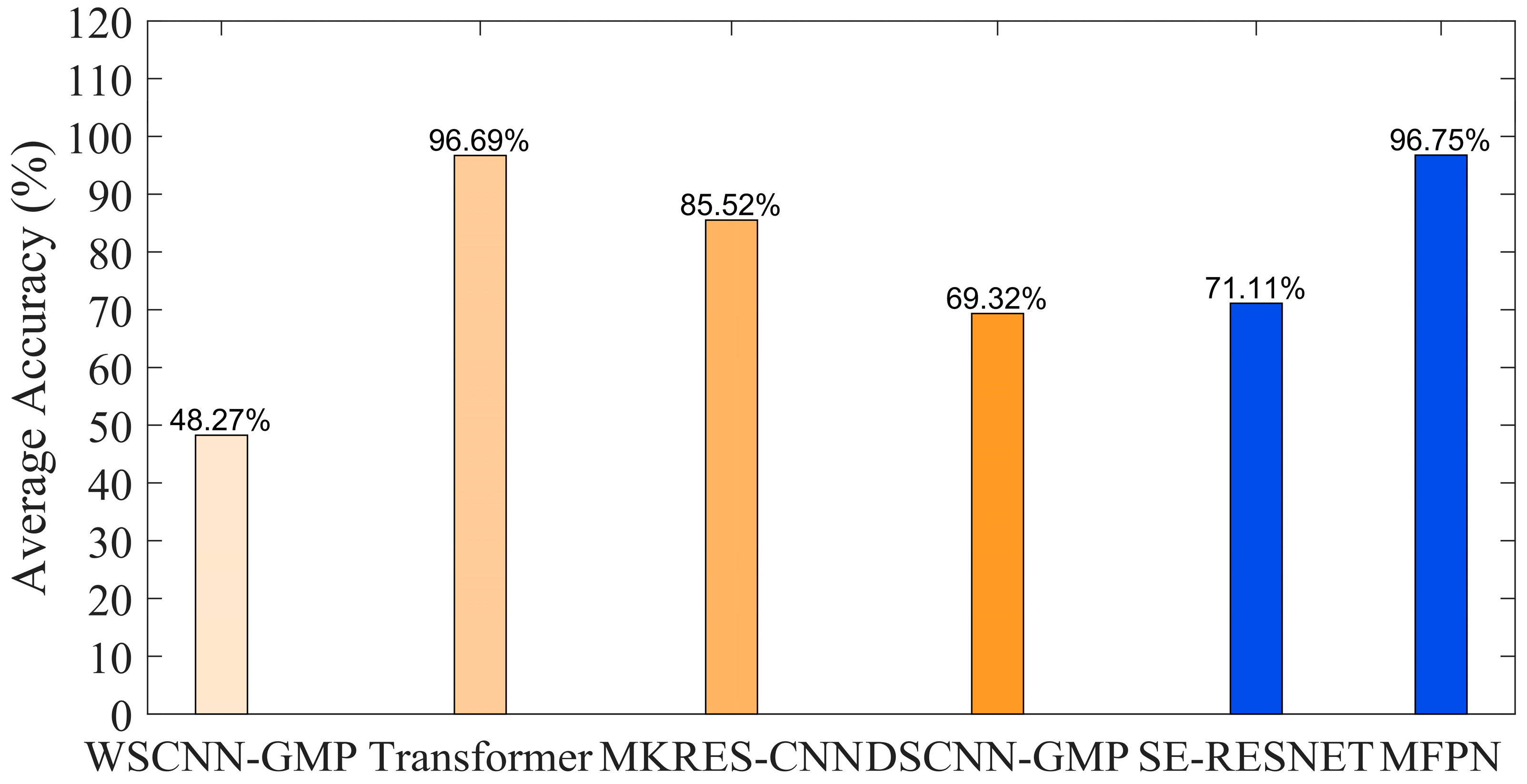
WSCNN-GMP [31]: WSCNN-GMP is an improved convolutional neural network-based method specifically designed for inverter fault diagnosis under varying load conditions;

(2)

TRANSFORMER [32]: The Transformer algorithm is a self-attention-based method developed for tasks involving long-range sequence processing;

(3)

MKRES-CNN [33]: MKRES-CNN is an algorithm based on a multiscale residual convolutional neural network designed explicitly for fault diagnosis of the motor;

(4)

DSCNN-GMP [33]: DSCNN-GMP is an algorithm based on depth-wise separable convolution with global max pooling, designed explicitly for open-circuit fault diagnosis of neutral-point clamped (NPC) inverters;

(5)

SE-ResNet [34]: SE-ResNet is an improved neural network algorithm based on ResNet, used for open-circuit fault diagnosis in photovoltaic inverters.

4.2. Comparison with Other Algorithm

To ensure the accuracy of the experimental data, each method was tested five times, and the average value was taken as the final result. Detailed results are shown in Figure 9. The study indicates that the proposed multi-dimensional feature perception network significantly outperforms other comparison algorithms under various operating conditions, achieving outstanding diagnostic performance. Even the worst result of MFPN exceeded the results of WSCNN-GMP, TRANSFORMER, MKRES-CNN, DSCNN-GMP, and SE-ResNet by 51.17%, 0.06%, 11.23%, 27.43%, and 28.33%, respectively.

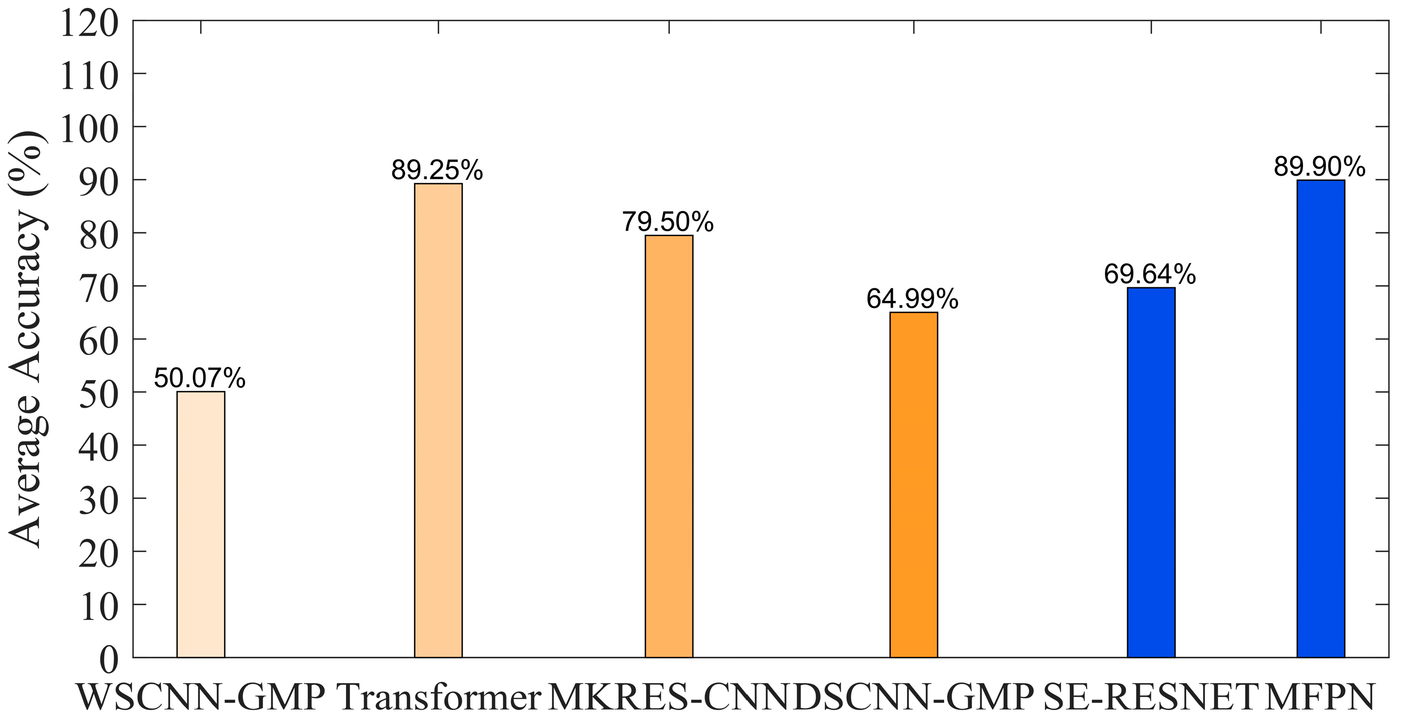
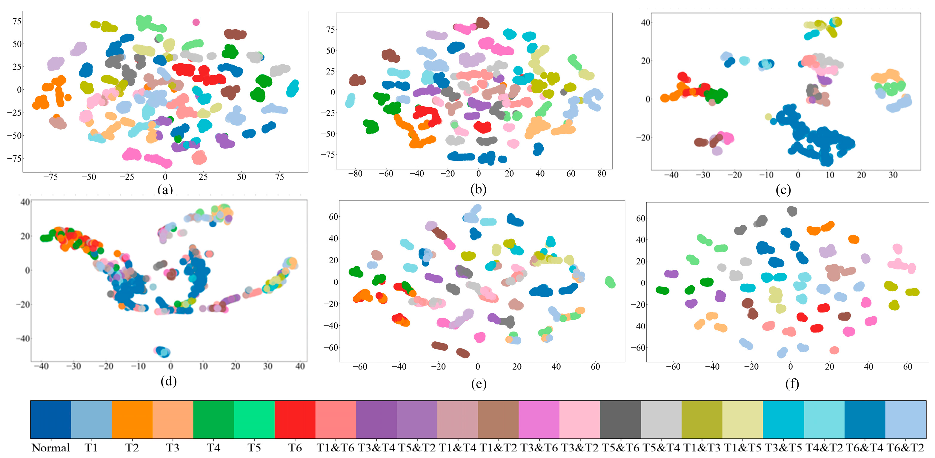
4.3. Robustness AGAINST Generalization Test

As shown in Figure 9, a generalization performance validation dataset was constructed under five different unseen weather conditions to effectively evaluate the diagnostic performance of the multi-dimensional feature perception network on this dataset. To ensure the accuracy of the experimental data, each method was tested five times, and the average value was taken as the final result. Figure 10 further verifies the robustness of the multi-dimensional feature perception network, whose superior feature extraction capability consistently outperformed the other seven methods under each operating condition, always achieving higher average accuracy. Specifically, MFPN achieved an accuracy of 89.90%, which was 49.9%, 0.65%, 10.4%, 24.91%, and 30.33% higher than the other seven methods, respectively. This further demonstrates that MFPN exhibits excellent generalization performance compared to other methods.

To better validate the interpretability of MFPN, t-SNE was employed to visualize the generalization test dataset. Figure 11 shows that MFPN excels at distinguishing between different classes. Notably, the feature maps generated by MFPN display distinct clusters for similar classes, with minimal overlap between different categories.

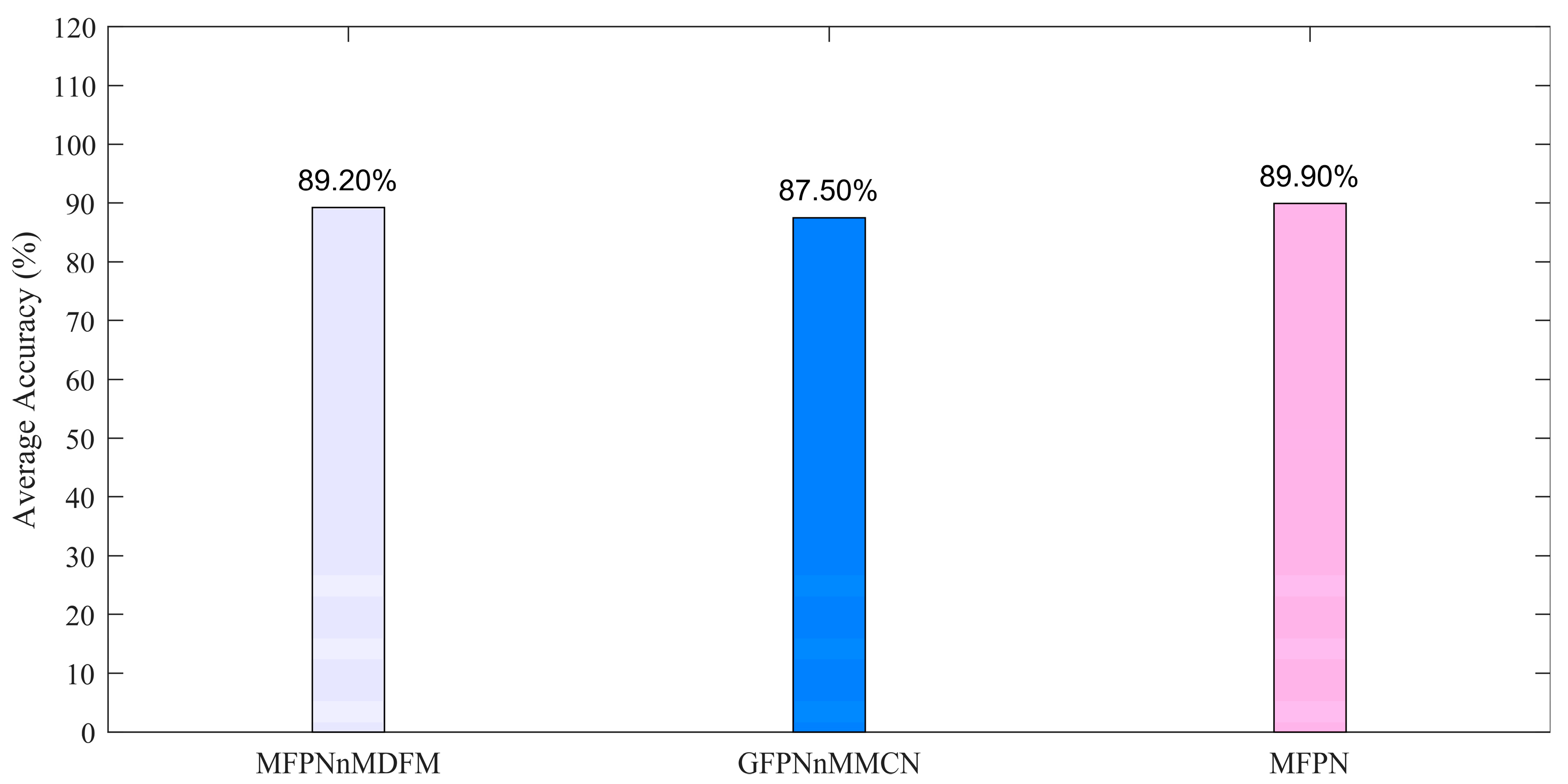
4.4. Ablidation Studies

This section experimentally evaluates the effectiveness of the multi-dimensional feature fusion module and the multi-head convolutional self-attention mechanism. MFPN-nMDFF removes the multi-dimensional feature fusion module, while MFPN-nMCAM adopts a traditional multi-head self-attention mechanism. These models share a similar structure with MFPN but differ in specific modules.

The ablation experiments were conducted on the generalization performance testing dataset, and the results are shown in Figure 12. Specifically, on the generalization performance dataset, MFPN achieved an accuracy of 89.90%, which was 2.4% and 0.7% higher than the other two methods, respectively. Therefore, our observations indicate that combining the multi-dimensional feature fusion module and the multi-head convolutional self-attention mechanism can enhance the fault diagnosis capability of MFPN.

4.5. Training Time, Inference Time, and Resource Usage Cost of the Models

To better compare the performance of MFPN in generalization scenarios, we evaluated the model using training time, inference time, and model complexity (FLOPs) (

Table 3. Comparison of model training time, inference time, and complexity.

Classifier	Training Time (s)	Inference Time (s)	FLOPs
WSCNN-GMP	35	0.176	3.40 × 109
Transformer	1320	0.215	29.2 × 109
MKRES-CNN	91	0.197	2.05 × 109
CNN-GAP	531	0.377	4.25 × 109
SE-RESNET	28	0.247	13.6 × 109
MFPN	1470	1.210	1.32 × 109

). The results show that although MFPN has the longest training time and the highest complexity, it still achieves the best accuracy. In summary, MFPN demonstrates the best performance across datasets from different scenarios.

5. Conclusions

This study focuses on the operating characteristics of PV grid-connected inverters under multiple working conditions and proposes a fault diagnosis model based on a multi-dimensional feature perception network. The model combines the strengths of the multi-dimensional feature mix module and the multi-scale convolutional Transformer. Compared with traditional methods, the proposed model demonstrates outstanding performance in PV inverter fault diagnosis, significantly improving diagnostic accuracy. Through fault diagnosis experiments under generalization performance scenarios, the results show that the multi-dimensional feature perception network maintains highly accurate and efficient diagnostic capabilities even in previously unseen conditions. The proposed model exhibits strong fault diagnosis capabilities and excellent robustness. Compared to other existing networks, the model achieves the highest fault diagnosis accuracy, offering a highly promising solution for the operation and maintenance of PV grid-connected inverters.

References

1. Bai, B.; Wang, Z.; Chen, J. Shaping the Solar Future: An Analysis of Policy Evolution, Prospects and Implications in China’s Photovoltaic Industry. Energy Strategy Rev. 2024, 54, 101474. [Google Scholar] [CrossRef]
2. De Almeida, J.O.M.B.; Torres, A.G.; Cupertino, A.F.; Pereira, H.A. Three-Phase Photovoltaic Inverters during Unbalanced Voltage Sags: Comparison of Control Strategies and Thermal Stress Analysis. In Proceedings of the 2016 12th IEEE International Conference on Industry Applications (INDUSCON), Curitiba, Brazil, 20–23 November 2016. [Google Scholar]
3. Meral, M.E.; Çelik, D. Minimisation of Power Oscillations with a Novel Optimal Control Strategy for Distributed Generation Inverter under Grid Faulty and Harmonic Networks. IET Renew. Power Gener. 2020, 14, 3010–3022. [Google Scholar] [CrossRef]
4. Chen, Y.; Liu, Z.; Chen, Z. Fast Diagnosis and Location Method for Open-Circuit Fault in Inverter Based on Current Vector Character Analysis. Trans. China Electrotech. Soc. 2018, 33, 883–891. [Google Scholar]
5. Bandyopadhyayi, P.; Purkait, P.; Koley, C. A SVM-Based Classifier for Identification of Spurious Resistance Fault Involving IGBTs in VSI-Based Induction Motor Drive. In Proceedings of the 2018 IEEE Applied Signal Processing Conference (ASPCON), Kolkata, India, 7–9 December 2018; pp. 9–13. [Google Scholar] [CrossRef]
6. Hu, K.; Meng, X.; Liu, Z.; Xu, J.; Lin, G.; Tong, L. Flux-Based Open-Switch Fault Diagnosis and Fault Tolerance for IM Drives with Predictive Torque/Flux Control. IEEE Trans. Transp. Electrif. 2022, 8, 4595–4606. [Google Scholar] [CrossRef]
7. Jlassi, I.; Estima, J.O.; El Khil, S.K.; Bellaaj, N.M.; Cardoso, A.J.M. Multiple Open-Circuit Faults Diagnosis in Back-to-Back Converters of PMSG Drives for Wind Turbine Systems. IEEE Trans. Power Electron. 2015, 30, 2689–2702. [Google Scholar] [CrossRef]
8. Campos-Delgado, D.U.; Espinoza-Trejo, D.R. An Observer-Based Diagnosis Scheme for Single and Simultaneous Open-Switch Faults in Induction Motor Drives. IEEE Trans. Ind. Electron. 2011, 58, 671–679. [Google Scholar] [CrossRef]
9. Espinoza-Trejo, D.R.; Campos-Delgado, D.U. Detection and Isolation of Actuator Faults for a Class of Nonlinear Systems with Application to Electric Motors Drives. IET Control Theory Appl. 2009, 3, 1317–1329. [Google Scholar] [CrossRef]
10. Champa, P.N.; Deshpande, A.A. Effect of LSPWM at Variable and Fixed Switching Frequency on Cascaded Multilevel Inverter. In Proceedings of the 2024 International Conference on Advances in Modern Age Technologies for Health and Engineering Science (AMATHE), Shivamogga, India, 16–17 May 2024; pp. 1–7. [Google Scholar] [CrossRef]
11. Shi, T.; He, Y.; Wang, T.; Tong, J.; Li, B.; Deng, F. An Improved Open-Switch Fault Diagnosis Technique of a PWM Voltage Source Rectifier Based on Current Distortion. IEEE Trans. Power Electron. 2019, 34, 12212–12225. [Google Scholar] [CrossRef]
12. Nzekwu, C.N. Fault Diagnosis of Inverter Power Switches Using Signal-Data Based Machine Learning. Doctoral Thesis, Glasgow Caledonian University, Glasgow, UK, 2024. [Google Scholar]
13. Martins, J.F.; Pires, V.F.; Lima, C.; Pires, A.J. Fault Detection and Diagnosis of Grid-Connected Power Inverters Using PCA and Current Mean Value. In Proceedings of the IECON 2012—38th Annual Conference of the IEEE Industrial Electronics Society, Montreal, QC, Canada, 25–28 October 2012; pp. 5185–5190. [Google Scholar] [CrossRef]
14. Khomfoi, S.; Tolbert, L.M. Fault Diagnosis and Reconfiguration for Multilevel Inverter Drive Using AI-Based Techniques. IEEE Trans. Ind. Electron. 2007, 54, 2954–2968. [Google Scholar] [CrossRef]
15. Ali, M.; Din, Z.; Solomin, E.; Cheema, K.M.; Milyani, A.H.; Che, Z. Open Switch Fault Diagnosis of Cascade H-Bridge Multi-Level Inverter in Distributed Power Generators by Machine Learning Algorithms. Energy Rep. 2021, 7, 8929–8942. [Google Scholar] [CrossRef]
16. Sun, Q.; Yu, X.; Li, H.; Fan, J. Adaptive Feature Extraction and Fault Diagnosis for Three-Phase Inverter Based on Hybrid-CNN Models under Variable Operating Conditions. Complex Intell. Syst. 2022, 8, 29–42. [Google Scholar] [CrossRef]
17. Li, B.; Lu, W.; Xie, Z. Open-Circuit Fault Diagnosis Method of ANPC Three-Level Inverter Based on Joint Optimized Echo State Network. In Proceedings of the 2023 IEEE 2nd International Power Electronics and Application Symposium (PEAS), Guangzhou, China, 10–13 November 2023; pp. 1912–1915. [Google Scholar] [CrossRef]
18. Li, J.; Tao, J.; Ding, W.; Zhang, J.; Meng, Z. Period-Assisted Adaptive Parameterized Wavelet Dictionary and Its Sparse Representation for Periodic Transient Features of Rolling Bearing Faults. Mech. Syst. Signal Process. 2022, 169, 108796. [Google Scholar] [CrossRef]
19. Fu, Y.; Ji, Y.; Meng, G.; Chen, W.; Bai, X. Three-Phase Inverter Fault Diagnosis Based on an Improved Deep Residual Network. Electronics 2023, 12, 3460. [Google Scholar] [CrossRef]
20. Jiang, W.; Tashakor, N.; Pourhadi, P.; Koehler, A.; Wang, H.; Goetz, S.M. Optimizing PV–Battery Hybrid Systems: A Reconfigurable Approach with Module-Level Maximum-Power-Point Tracking and Load Sharing. IEEE Trans. Power Electron. 2024, 40, 2327–2341. [Google Scholar] [CrossRef]
21. Feng, X.; Yan, Z.; Chen, N.; Zhang, Y.; Ma, Y.; Liu, X.; Fan, Q.; Wang, L.; Huang, W. The Synthesis of Shape-Controlled MnO2/Graphene Composites via a Facile One-Step Hydrothermal Method and Their Application in Supercapacitors. J. Mater. Chem. A1 2013, 1, 12818–12825. [Google Scholar] [CrossRef]
22. Li, Y.; Dai, W.; Zhang, W. Bearing Fault Feature Selection Method Based on Weighted Multidimensional Feature Fusion. IEEE Access 2020, 8, 19008–19025. [Google Scholar] [CrossRef]
23. Han, T.; Liu, C.; Wu, L.; Sarkar, S.; Jiang, D. An Adaptive Spatiotemporal Feature Learning Approach for Fault Diagnosis in Complex Systems. Mech. Syst. Signal Process. 2019, 117, 170–187. [Google Scholar] [CrossRef]
24. Liu, H.; Xu, Q.; Han, X.; Wang, B.; Yi, X. Attention on the Key Modes: Machinery Fault Diagnosis Transformers through Variational Mode Decomposition. Knowl.-Based Syst. 2024, 289, 111479. [Google Scholar] [CrossRef]
25. Yan, X.; Li, Z.; Meng, L.; Qi, Z.; Wu, W.; Li, Z.; Meng, X. Empowering Vision Transformers with Multi-Scale Causal Intervention for Long-Tailed Image Classification. arXiv 2025, arXiv:2505.08173. [Google Scholar]
26. Mao, J.; Jain, A.K. Artificial Neural Networks for Feature Extraction and Multivariate Data Projection. IEEE Trans. Neural Netw. 1995, 6, 296–317. [Google Scholar] [CrossRef] [PubMed]
27. Yang, J.; Lee, C.-H. Real-Time Data-Driven Method for Bolt Defect Detection and Size Measurement in Industrial Production. Actuators 2025, 14, 185. [Google Scholar] [CrossRef]
28. Urrea, C. Hybrid Fault-Tolerant Control in Cooperative Robotics: Advances in Resilience and Scalability. Actuators 2025, 14, 177. [Google Scholar] [CrossRef]
29. Wu, Y.; Wu, Z. A Generalized Center-Aligned High-Resolution Pulse Width Modulator Implementation Using an Output Serializer in Field Programmable Gate Arrays. Actuators 2025, 14, 181. [Google Scholar] [CrossRef]
30. Zhang, W.; Guo, F. Research on Sensorless Technology of a Magnetic Suspension Flywheel Battery Based on a Genetic BP Neural Network. Actuators 2025, 14, 174. [Google Scholar] [CrossRef]
31. Zhang, S.; Wang, R.; Si, Y.; Wang, L. An Improved Convolutional Neural Network for Three-Phase Inverter Fault Diagnosis. IEEE Trans. Instrum. Meas. 2022, 71, 3510915. [Google Scholar] [CrossRef]
32. Lv, H.; Chen, J.; Pan, T.; Zhang, T.; Feng, Y.; Liu, S. Attention Mechanism in Intelligent Fault Diagnosis of Machinery: A Review of Technique and Application. Measurement 2022, 199, 111594. [Google Scholar] [CrossRef]
33. Xie, F.; Tang, X.; Xiao, F.; Luo, Y.; Shen, H.; Shi, Z. Online Diagnosis Method for Open-Circuit Fault of NPC Inverter Based on 1D-DSCNN-GMP Lightweight Edge Deployment. IEEE J. Emerg. Sel. Top. Power Electron. 2023, 11, 6054–6067. [Google Scholar] [CrossRef]
34. Lin, P.; Qian, Z.; Lu, X.; Lin, Y.; Lai, Y.; Cheng, S.; Chen, Z.; Wu, L. Compound Fault Diagnosis Model for Photovoltaic Array Using Multi-Scale SE-ResNet. Sustain. Energy Technol. Assess. 2022, 50, 101785. [Google Scholar] [CrossRef]
Figure 1. Infrastructure of PV grid-connected inverter.
Energies 18 04044 g001
Figure 2. (a) Single-switch fault. (b) Double-switch fault on different phase leg. (c) Double-switch fault on the same phase leg but different phase. (d) Double-switch fault on the same phase.
Energies 18 04044 g002
Figure 3. (a) T1 open-switch fault. (b) T1&T2 open-switch fault. (c) T1&T3 open-switch fault. (d) T1&T6 open-switch fault.
Energies 18 04044 g003
Figure 4. Architecture of MFPN. The MFPN comprises two core components: MDFM and MDC-Former. MDFM is augmented by AFPM, while MDC-Former is enhanced through MCA, which is further optimized by MFMM. (A) Dataset processing. (B) Fault diagnosis based on MFPN. (C) Results display.
Energies 18 04044 g004
Figure 5. (a) Adaptive feature perception module. (b) Multi-scale feature mix module.
Energies 18 04044 g005
Figure 6. (a) Multi-scale convolution self-attention. (b) Multi-head MCA. (c) MDC-Former.
Energies 18 04044 g006
Figure 7. HIL platform for PV grid-connected system. (a) Platform configuration. (b) Detailed implementation.
Energies 18 04044 g007
Figure 8. P–V curve of the training dataset and generalization dataset.
Energies 18 04044 g008
Figure 9. Diagnostic results of the HIL platform dataset.
Energies 18 04044 g009
Figure 10. Diagnostic results for generalization test of the HIL platform dataset.
Energies 18 04044 g010
Figure 11. Feature visualization of t-SNE for HIL platform generalization test dataset: (a) WSCNN-GMP, (b) Transformer, (c) MKRES-CNN, (d) DSCNN-GMP, (e) SE-RESNET, (f) MFPN.
Energies 18 04044 g011
Figure 12. Diagnostic results for generalization test of the ablidation study.
Energies 18 04044 g012