Modeling Biomass Conversion in Raceway Zone of Blast Furnace Using Resolved Lagrangian Particle Model

Abstract

This study numerically investigates the suitability of biomass particles of varying diameters as alternative reducing agents in the blast furnace raceway zone, where harsh conditions can create internal gradients affecting conversion. An internally resolved 1D Lagrangian particle model, fully integrated into the open-source CFD toolbox OpenFOAM^®, is used to model temperature and species gradients within thermally thick particles. The particle model is coupled with the surrounding Eulerian phase and includes drying, pyrolysis, oxidation, and gasification submodels. Results show that only biomass particles smaller than 250 μm fully convert in the raceway, while larger particles carry unconverted material beyond, potentially reducing blast furnace efficiency.

1. Introduction

The reduction of CO₂ emissions is an important global goal. The steel industry accounts for about 7% of the global CO₂ emissions [1]. A possible way to reduce the CO₂ emissions in the steel industry is to utilize biomass as an alternative to fossil fuels. Possible uses of biomass in the steel industry range from using biomass in iron ore pellets, to replace metallurgical coke or as an alternative reducing agent (ARA) in the raceway zone (RW) of the blast furnace (BF) to reducing the metallurgical coke consumption [2,3,4,5].

Computational fluid dynamics (CFD) simulations are a promising tool for investigating potential ARAs, e.g., biomass or plastic pellets, because it is difficult to experimentally explore RW conditions, due to the high pressures and temperatures involved [6]. A possible issue with using biomass as ARAs is that the size distribution of ground biomass tends to be larger than that of pulverized coal. This can lead to incomplete conversion inside the RW for large biomass particles [7]. Incomplete conversion can lead to clogging of the BF and prevent the desired reduction in CO₂ emissions and increase in BF efficiency [8,9].

In order to make predictions about the conversion behavior of biomass as ARAs and their interactions with the surrounding gas phase, it is essential to choose a modeling approach that fits the given problem. The thermochemical ARA particle conversion depends on several complex physical phenomena. These phenomena include but are not limited to the internal particle temperature and species composition, the energy and species release from the particles, the gas composition and temperature changes surrounding the particles, the interaction between particles, and the trajectories of the particles after injection into the RW [10,11]. A wide variety of particle models to simulate and predict the thermochemical conversion behavior of solid fuel particles were proposed in the literature. These models feature different levels of complexity, ranging from fully resolved 3D particles to single 0D point particles. Fully resolved 2D and 3D particle models, e.g., [12,13,14,15,16], model detailed internal particle structures and use detailed reaction mechanisms inside the particle. Detailed analyses of the processes and changes in the internal particle states during the thermochemical conversion of single particles can be performed with these models. However, this comes at the cost of high computational complexity. Generally, fully resolved 2D and 3D particle models are only used to simulate single particles. These models commonly split the problem into two regions (particle and surrounding gas phase) that interact via region coupling boundary conditions (BC) [17]. While these models have no limitations regarding the initial particle size and shape, modeling changes in the particle size, shape, and position can be numerically too expensive to include. Therefore, these models usually ignore important phenomena like shrinking or swelling.

Lagrangian 0D point particle models, e.g., [10,18,19,20] use simple reaction, heat, and mass transfer equations while allowing for a large number of particles to be simulated simultaneously due to low computational costs. The particles can move through the simulation domain according to Newton’s laws of motion, depending on the Eulerian flow field. The particles can also exchange source terms with the Eulerian phase. However, it is not possible to resolve internal gradients inside the particles with these models. Therefore, non-isothermal behavior of large particles can not be modeled [21,22].

Another type of particle models is 1D internally resolved models. In general 1D models represent particles with radially symmetric shapes by reducing them to homogeneous layers, e.g., [23,24,25,26,27,28,29]. One-dimensional models can depict complex internal particle states, including internal gradients for energy and species concentration, and, therefore, can include more complex reaction mechanisms and reproduce more complex behavior. These models are less precise than resolved 3D models but are numerically much less expensive to solve. While some 1D models are standalone models and not integrated into a larger-scale CFD simulation, the resolved Lagrangian particle model (RLPM) used in this work is integrated into the open source CFD toolbox OpenFOAM^® [30] (OF). The RLPM can be used inside Eulerian-CFD simulations in OpenFOAM^® the same way as existing unresolved Lagrangian models. This allows for the modeling of complex, non-isothermal conversion behavior, as well as the trajectories of the particles after injection. The RLPM is suited to investigate the conversion of larger particles in complex systems, i.e., the ARA conversion in the RW of the BF.

In this work we first describe the mathematical foundation of the RLPM. The RLPM is then applied to study the thermochemical conversion of biomass particles with different diameters in the RW zone of the BF. The conversion behavior is investigated by injecting 1000 particles for each of 9 diameters into a frozen RW CFD simulation. The conversion behavior along the particle radius of the different particle sizes is assessed and compared to the corresponding particle Biot numbers, Stokes numbers, and average trajectories through the RW zone. The study is concluded by assessing a maximum particle diameter above which unconverted biomass is transported out of the RW.

2. Model Theory

The resolved Lagrangian particle model (RLPM) has been previously used to investigate thermally thick behavior inside the raceway zone of the blast furnace [7]. In the following section the model theory is summarized.

The RLPM is based on the same framework as the unresolved Lagrangian particle models in the open source CFD toolbox OpenFOAM^® and is natively implemented in OpenFOAM^® version 9 [30]. The RLPM is internally resolved by a 1D grid, and on this 1D grid, temperature and species concentration profiles can be calculated inside the particle. This enables the modeling of large particles that can develop significant internal gradients (thermally thick behavior), while 0D models are restricted to smaller particle sizes. From the Eulerian carrier phase’s point of view, the internally resolved particle is still a 0D point and interacts with the Eulerian carrier phase only via source terms for energy, species mass, and momentum.

The internal 1D resolution assumes a radially symmetrical particle that can be reduced to homogeneous, concentric layers. Each layer is represented by a single grid point located in the center of the layer. In order to model simple geometries, like spheres, cylinders, or slabs, a geometric factor $\Gamma \left(r\right)$ is introduced to the transport equations by modifying each volume element as $dV=\Gamma \left(r\right)·dr$ [31]. For the spherical particles investigated in this study $\Gamma \left(r\right)=4\pi r^2$ and the finite difference approximation of $\Gamma \left(r\right)·dr$ is of the form:

$$\Gamma \left(r\right)·dr\approx {\displaystyle \frac{4}{3}}\pi ·\left(r_l^3-r_{l-1}^3\right),$$

(1)

where $r_l$ and $r_{l-1}$ are distances from the particle center to the middle of the layers with index l and $l-1$. The layer indices go from $l=0$ (layer closest to particle center) to $l=N_l$ (layer closest to particle surface), with $N_l$ being equal to the number of layers.

The RLPM is a multiphase model consisting of a gas, a solid, and a liquid phase. All three phases have associated mass fractions, species compositions, heat capacities, thermal conductivities, and masses in each layer. Only the gas phase can move throughout the particle and into the carrier phase. The solid phase is a stationary matrix, and the liquid phase is assumed to be bound to the solid. Therefore, the mass transport equations are only solved for gas phase species. The energy transport equation is solved for all three phases combined, resulting in a single temperature value for each grid point inside the particle.

The mass transport equation is solved independently for each gas phase species using an effective diffusion coefficient $D_{\mathrm{eff},i}$ for each species i in the mixture [32,33]:

$$D_{\mathrm{eff},i}={\displaystyle \frac{ϵ}{\tau }}{D}_i\approx {ϵ}^2{D}_i,$$

(2)

where $\tau$ is the tortuosity, $ϵ$ is the porosity, and $D_i$ is the molecular diffusivity of gas phase species i, that can be calculated as follows:

$${\displaystyle \frac{1}{D_i}}={\displaystyle \frac{1}{D_{ij}}}+{\displaystyle \frac{1}{D_{Ki}}},$$

(3)

where $D_{ij}$ is the binary diffusion coefficient, and $D_{Ki}$ is the Knudsen diffusion coefficient. In this form the binary diffusion coefficient and the Knudsen coefficient are arranged as a parallel resistor network to yield the molecular diffusivity. This applies in the transition regime between Knudsen and bulk diffusion, which often occurs in pores. Therefore, the limiting factor of the diffusivity depends on whether the probability of binary molecular collisions is larger (Bulk Diffusion Regime) or smaller than the probability of wall-molecule collisions (Knudsen Diffusion Regime). The mass transport equation for the molar concentration $C_i$ of species i, including the geometric factor $\Gamma \left(r\right)$, is of the following form:

$${\displaystyle \frac{\partial C_i}{\partial t}}={\displaystyle \frac{1}{\Gamma \left(r\right)}}{\displaystyle \frac{\partial }{\partial x}}\left(D_{\mathrm{eff},i}\Gamma \left(r\right){\displaystyle \frac{\partial C_i}{\partial x}}\right)+S_{C_i}.$$

(4)

Here $S_{C_i}$ is the mass source for each species i, due to chemical conversion.

An advective BC couples the mass transport inside the RLPM with the Eulerian carrier phase at the particle surface ($r=R$) using the carrier phase molar concentration $C_{iC}$ of species i interpolated to the particle surface:

$$D_{\mathrm{eff},i}·{\displaystyle \frac{\partial C_i}{\partial r}}{|}_{r=R}=-h_m·(C_{iC}-C_i).$$

(5)

The mass transfer coefficient $h_m$ is calculated using the Frossling correlation [34].

The energy transport equation has a form similar to the mass transport equation:

$${\displaystyle \frac{\partial T}{\partial t}}={\displaystyle \frac{1}{\rho {\mathrm{c}}_{\mathrm{p},\mathrm{eff}}\Gamma \left(r\right)}}{\displaystyle \frac{\partial }{\partial x}}\left({\kappa }_{\mathrm{eff}}\Gamma \left(r\right){\displaystyle \frac{\partial T}{\partial x}}\right)+S_T,$$

(6)

where ${\kappa }_{\mathrm{eff}}$ and ${\mathrm{c}}_{\mathrm{p},\mathrm{eff}}$ are the mass-fraction averaged effective thermal conductivity and effective heat capacity for the mixture of all solid species inside the particle. T is the temperature, $\rho$ is the particle density, and $S_T$ is the energy source due to chemical reactions. The heat transport equation is coupled to the carrier phase using a combined advective and radiative BC:

$${\displaystyle \frac{{\kappa }_{\mathrm{eff}}}{\rho {\mathrm{c}}_{\mathrm{p},\mathrm{eff}}}}·{\displaystyle \frac{\partial T}{\partial r}}{|}_{r=R}=-h·(T_C-T)-\sigma \epsilon ·(T_C^4-T^4).$$

(7)

Here $T_C$ is the carrier phase temperature at the particle surface, h is the heat transfer coefficient calculated according to the Ranz-Marshall correlation [35], $\sigma$ is the Stefan-Boltzmann constant, and $\epsilon$ is the emission coefficient.

The mass and energy transport equations only consider diffusive transport while neglecting convective transport for numerical efficiency. This simplification can cause prediction errors for high moisture contents and fast pyrolysis conditions, since convective fluxes can exceed diffusive ones under these conditions. For the transport equation’s numerical solution, spatial gradients are discretized using second-order finite differences, while time integration uses an implicit Euler scheme. The implicit integration allows for stable solutions at large time steps and ensures the conservation of mass and energy inside the particle.

The thermochemical conversion submodels inside the RLPM are solved by accessing each grid point’s pressure, temperature, and species concentrations. Three chemistry submodels are subsequently solved:

• Drying (Liquid → Gas);
• Pyrolysis (Solid → Solid + Gas);
• Oxidation and Gasification (Solid + Gas → Gas).

Inside the particle, gas phase chemistry is neglected, and only heterogeneous reactions are considered.

Drying is modeled via thermal drying according to [36], using the definition of a threshold temperature $T_{\mathrm{evap}}$, which depends on the carrier phase pressure interpolated to the particle surface $p_C$:

$$T_{\mathrm{evap}}=32.7·\log \left({\displaystyle \frac{p_C}{101325}}\right)+373.15.$$

(8)

Once the particle temperature $T_l$ in layer l exceeds the threshold temperature $T_{\mathrm{evap}}$, the evaporation mass change $\Delta m_{\mathrm{evap},l}$ is calculated as follows:

$$\Delta m_{\mathrm{evap},l}=\min \left({\displaystyle \frac{F_{\mathrm{Heat},l}}{\Delta h_{\mathrm{evap}}}}·f_{\mathrm{evap}}·\Delta t,m_{{\mathrm{H}}_2\mathrm{O},\mathrm{Liq},l}\right),$$

(9)

where $F_{\mathrm{Heat},l}$ is the incoming heat flux into layer l, $\Delta h_{\mathrm{evap}}$ is the evaporation enthalpy, $m_{{\mathrm{H}}_2\mathrm{O},\mathrm{Liq},l}$ is the total remaining moisture mass in layer l, which limits the evaporation mass, and $\Delta t$ is the time step size. The evaporation efficiency $f_{\mathrm{evap}}$ determines the share of the heat flux used for drying. If $f_{\mathrm{evap}}=1$ the complete heat flux is used for drying, and the particle temperature cannot rise above $T_{\mathrm{evap}}$ until all water has evaporated.

For pyrolysis a model similar to the one described in [37] is employed. It assumes a one-step mechanism for decomposing each of the three pseudo-components of biomass: cellulose, hemicellulose, and lignin. This one-step mechanism is modeled according to a first-order Arrhenius approach and results in the change in mass $\Delta m_{\mathrm{pyro},i,l}$ of biomass component i in layer l:

$$\Delta m_{\mathrm{pyro},i,l}=min\left(m_{i,l}{A}_i{\mathrm{e}}^{-E_{a,i}/\left(R{T}_l\right)}\Delta t,m_{i,l}\right),$$

(10)

where R is the ideal gas constant, $m_{i,l}$ is the mass of solid biomass component i in layer l, $T_l$ is the temperature of layer l, $E_{a,i}$ is the activation energy for component i, $A_i$ is the pre-exponential factor for component i, and $\Delta t$ is the time step size.

The oxidation and gasification models describe the heterogeneous gas–solid reactions depending on the partial pressure $p_{i,l}$ of the gas phase educts and internal particle surface $A_{p,l}$, for each layer l:

$$\Delta m_{\mathrm{het},i,l}=min\left(A_{p,l}{p}_{i,l}{A}_i·\exp \left(-{\displaystyle \frac{E_{a,i}}{R{T}_l}}\right)\Delta t,m_{i,l}\right),$$

(11)

Reactions at the outer surface lead to particle shrinking, while reactions inside the particle lead to an increase in porosity.

Because the particles can be larger than a single cell size in the simulations, a simple mapping algorithm is applied to spread the particle source terms onto all cells covered by the particle. The algorithm is similar to the moving average method proposed by [29], but the distribution volume is limited to cells that overlap with the particle. It uses a constant source density approach to distribute the particle source terms onto the Eulerian phase.

3. Model Parameters for Biomass

The RLPM parameters to model biomass conversion are chosen from Lu et al., as well as Mehrabian et al. [23,25]. Both groups studied the single particle conversion behavior of biomass extensively using the presented parameters.

Table 1 summarizes the physical particle properties used in the simulations, while Table 2 lists the thermo-physical transport properties of the gas and solids.

The solid biomass is modeled as consisting of three pseudo-components: cellulose, hemicellulose, and lignin. The three components have different reaction kinetics, which are used to model the complex pyrolysis behavior of biomass via a global mechanism [37].

The carrier phase properties were taken from the GRI3.0 mechanism [38].

The drying submodel uses a drying efficiency $f_{\mathrm{evap}}=1$ to best recreate the experimental results used for validation. Table 3 lists the pyrolysis reactions and their parameters, and Table 4 lists the pyrolysis product composition, which is identical for cellulose, hemicellulose, and lignin. Table 5 lists the reaction parameters of the oxidation and gasification reactions of the resulting char content.

Table 1. Summary of physical particle properties. Wood is used whenever hemicellulose, cellulose, and lignin have the same properties.

Property	Value	Unit	Ref.
particle shape	sphere	-	-
initial mass fractions Y		kg/kg
$Y_{\mathrm{hemicellulose}}$	0.2587	w.r.t. dry mass	[37]
$Y_{\mathrm{cellulose}}$	0.6368	w.r.t. dry mass	[37]
$Y_{\mathrm{lignin}}$	0.0995	w.r.t. dry mass	[37]
$Y_{\mathrm{ash}}$	0.005	w.r.t. dry mass	[37]
$Y_{\mathrm{water}}$	0.08	w.r.t. wet mass	[10]
initial porosity $ϵ$	0.4	-	[23]
density $\rho$		kg/m3
${\rho }_{\mathrm{wood}}$	580		[23]
${\rho }_{\mathrm{char}}$	200		[39]
${\rho }_{\mathrm{ash}}$	300		[25]
pore diameter $d_{pore}$	$3.2·{10}^{-6}$	m	[23]
binary diffusion coefficient $D_{ab}$	$3·{10}^{-5}$ for all species	m2/s	[23]
char inner surface	$1·{10}^6$	m2/m3	[23]
particle diameter $d_p$	$9.5$	mm	[23]

Table 1. Summary of physical particle properties. Wood is used whenever hemicellulose, cellulose, and lignin have the same properties.

Property	Value	Unit	Ref.
particle shape	sphere	-	-
initial mass fractions Y		kg/kg
$Y_{\mathrm{hemicellulose}}$	0.2587	w.r.t. dry mass	[37]
$Y_{\mathrm{cellulose}}$	0.6368	w.r.t. dry mass	[37]
$Y_{\mathrm{lignin}}$	0.0995	w.r.t. dry mass	[37]
$Y_{\mathrm{ash}}$	0.005	w.r.t. dry mass	[37]
$Y_{\mathrm{water}}$	0.08	w.r.t. wet mass	[10]
initial porosity $ϵ$	0.4	-	[23]
density $\rho$		kg/m3
${\rho }_{\mathrm{wood}}$	580		[23]
${\rho }_{\mathrm{char}}$	200		[39]
${\rho }_{\mathrm{ash}}$	300		[25]
pore diameter $d_{pore}$	$3.2·{10}^{-6}$	m	[23]
binary diffusion coefficient $D_{ab}$	$3·{10}^{-5}$ for all species	m2/s	[23]
char inner surface	$1·{10}^6$	m2/m3	[23]
particle diameter $d_p$	$9.5$	mm	[23]

Table 2. Summary of thermo-physical particle properties. Wood is used whenever hemicellulose, cellulose, and lignin have the same properties.

Property	Value	Unit	Ref.
heat capacity $c_{\mathrm{p}}$		J/kg/K
$c_{\mathrm{p},\mathrm{wood}}$	$1000R/7.72·\left(g(380/T)+2g(1800/T)\right)$		[40]
$c_{\mathrm{p},\mathrm{char}}=c_{\mathrm{p},\mathrm{ash}}$	$1000R/11.3·\left(g(380/T)+2g(1800/T)\right)$		[40]
	with $g\left(x\right)=x^2{\mathrm{e}}^x/{\left({\mathrm{e}}^x-1\right)}^2$ and $R=8.314$ J/K/mol
thermal conductivity $\kappa$		W/m/K
${\kappa }_{\mathrm{wood}}$	$1.75·(0.129-0.049Y_{\mathrm{water}})·(1+(2.05+4Y_{\mathrm{water}})·{10}^{-3}·(T-273.15))·(0.986+2.695Y_{\mathrm{water}})$		[41]
${\kappa }_{\mathrm{char}}$	0.071		[23]
${\kappa }_{\mathrm{conduction}}$	$ϵ{\kappa }_{\mathrm{gas}}+(1-ϵ)\left(Y_{\mathrm{wood}}{\kappa }_{\mathrm{wood}}+Y_{\mathrm{char}}{\kappa }_{\mathrm{char}}\right)$
${\kappa }_{\mathrm{radiation}}$	$ϵ\sigma T^3{d}_{\mathrm{pore}}/\epsilon$
	with $\sigma =5.67·{10}^{-8}$ W/m2/K4
${\kappa }_{\mathrm{eff}}$	${\kappa }_{\mathrm{cond}}+{\kappa }_{\mathrm{rad}}$
emissivity $\epsilon$		-
${\epsilon }_{\mathrm{wood}}$	0.85		[23]
${\epsilon }_{\mathrm{char}}$	0.95		[23]
${\epsilon }_{\mathrm{ash}}$	0.75		[23]

Table 2. Summary of thermo-physical particle properties. Wood is used whenever hemicellulose, cellulose, and lignin have the same properties.

Property	Value	Unit	Ref.
heat capacity $c_{\mathrm{p}}$		J/kg/K
$c_{\mathrm{p},\mathrm{wood}}$	$1000R/7.72·\left(g(380/T)+2g(1800/T)\right)$		[40]
$c_{\mathrm{p},\mathrm{char}}=c_{\mathrm{p},\mathrm{ash}}$	$1000R/11.3·\left(g(380/T)+2g(1800/T)\right)$		[40]
	with $g\left(x\right)=x^2{\mathrm{e}}^x/{\left({\mathrm{e}}^x-1\right)}^2$ and $R=8.314$ J/K/mol
thermal conductivity $\kappa$		W/m/K
${\kappa }_{\mathrm{wood}}$	$1.75·(0.129-0.049Y_{\mathrm{water}})·(1+(2.05+4Y_{\mathrm{water}})·{10}^{-3}·(T-273.15))·(0.986+2.695Y_{\mathrm{water}})$		[41]
${\kappa }_{\mathrm{char}}$	0.071		[23]
${\kappa }_{\mathrm{conduction}}$	$ϵ{\kappa }_{\mathrm{gas}}+(1-ϵ)\left(Y_{\mathrm{wood}}{\kappa }_{\mathrm{wood}}+Y_{\mathrm{char}}{\kappa }_{\mathrm{char}}\right)$
${\kappa }_{\mathrm{radiation}}$	$ϵ\sigma T^3{d}_{\mathrm{pore}}/\epsilon$
	with $\sigma =5.67·{10}^{-8}$ W/m2/K4
${\kappa }_{\mathrm{eff}}$	${\kappa }_{\mathrm{cond}}+{\kappa }_{\mathrm{rad}}$
emissivity $\epsilon$		-
${\epsilon }_{\mathrm{wood}}$	0.85		[23]
${\epsilon }_{\mathrm{char}}$	0.95		[23]
${\epsilon }_{\mathrm{ash}}$	0.75		[23]

Table 3. Biomass pyrolysis reaction parameters, their pre-exponential factors A, and activation energies $E_a$. Pyrolysis gas composition is listed in Table 4.

	Pyrolysis Reaction	A [1/s]	${\mathbf{E}}_{\mathbf{a}}$ [J/kmol]	Ref.
R1	Hemicellulose $\to$ Cs + pyrolysis gas	$2.53·{10}^{11}$	$1.47·{10}^8$	[37]
R2	Cellulose $\to$ Cs + pyrolysis gas	$1.38·{10}^{14}$	$1.93·{10}^8$	[37]
R3	Lignin $\to$ Cs + pyrolysis gas	$2.2·{10}^{12}$	$1.81·{10}^8$	[37]

Table 3. Biomass pyrolysis reaction parameters, their pre-exponential factors A, and activation energies $E_a$. Pyrolysis gas composition is listed in Table 4.

	Pyrolysis Reaction	A [1/s]	${\mathbf{E}}_{\mathbf{a}}$ [J/kmol]	Ref.
R1	Hemicellulose $\to$ Cs + pyrolysis gas	$2.53·{10}^{11}$	$1.47·{10}^8$	[37]
R2	Cellulose $\to$ Cs + pyrolysis gas	$1.38·{10}^{14}$	$1.93·{10}^8$	[37]
R3	Lignin $\to$ Cs + pyrolysis gas	$2.2·{10}^{12}$	$1.81·{10}^8$	[37]

Table 4. Pyrolysis product composition from Lu et al. [23]. Light hydrocarbons have been modeled as ${\mathrm{CH}}_4$ in the simulation, according to Mehrabian et al. $C_s$ denotes solid carbon [25].

Species	${\mathbf{H}}_{\mathbf{2}}$	CO	${\mathbf{CO}}_{\mathbf{2}}$	${\mathbf{H}}_{\mathbf{2}}\mathbf{O}$	${\mathbf{CH}}_{\mathbf{4}}$	${\mathbf{C}}_{\mathbf{s}}$
mass fraction	0.114	0.356	0.188	0.018	0.224	0.095

Table 4. Pyrolysis product composition from Lu et al. [23]. Light hydrocarbons have been modeled as ${\mathrm{CH}}_4$ in the simulation, according to Mehrabian et al. $C_s$ denotes solid carbon [25].

Species	${\mathbf{H}}_{\mathbf{2}}$	CO	${\mathbf{CO}}_{\mathbf{2}}$	${\mathbf{H}}_{\mathbf{2}}\mathbf{O}$	${\mathbf{CH}}_{\mathbf{4}}$	${\mathbf{C}}_{\mathbf{s}}$
mass fraction	0.114	0.356	0.188	0.018	0.224	0.095

Table 5. Heterogeneous gas–solid particle reactions, their pre-exponential factors A, and activation energies $E_a$. $C_s$ denotes solid carbon.

	Heterogeneous Reaction	A [kmol/${\mathbf{m}}^2$/s/Pa]	${\mathbf{E}}_{\mathbf{a}}$ [J/kmol]	Ref.
R4	Cs + ${\displaystyle \frac{1}{2}}{\mathrm{O}}_2\to$ CO	$2.51·{10}^{-3}$	$7.48·{10}^7$	[42]
R5	Cs + ${\mathrm{CO}}_2\to$ 2CO	$0.0244$	$1.75·{10}^8$	[43]
R6	Cs + ${\mathrm{H}}_2\mathrm{O}\to \mathrm{CO}+{\mathrm{H}}_2$	$0.0244$	$1.75·{10}^8$	[43]
R7	Cs + $2{\mathrm{H}}_2\to {\mathrm{CH}}_4$	$1.18·{10}^{-6}$	$1.49·{10}^8$	[43]

Table 5. Heterogeneous gas–solid particle reactions, their pre-exponential factors A, and activation energies $E_a$. $C_s$ denotes solid carbon.

	Heterogeneous Reaction	A [kmol/${\mathbf{m}}^2$/s/Pa]	${\mathbf{E}}_{\mathbf{a}}$ [J/kmol]	Ref.
R4	Cs + ${\displaystyle \frac{1}{2}}{\mathrm{O}}_2\to$ CO	$2.51·{10}^{-3}$	$7.48·{10}^7$	[42]
R5	Cs + ${\mathrm{CO}}_2\to$ 2CO	$0.0244$	$1.75·{10}^8$	[43]
R6	Cs + ${\mathrm{H}}_2\mathrm{O}\to \mathrm{CO}+{\mathrm{H}}_2$	$0.0244$	$1.75·{10}^8$	[43]
R7	Cs + $2{\mathrm{H}}_2\to {\mathrm{CH}}_4$	$1.18·{10}^{-6}$	$1.49·{10}^8$	[43]

4. Model Validation

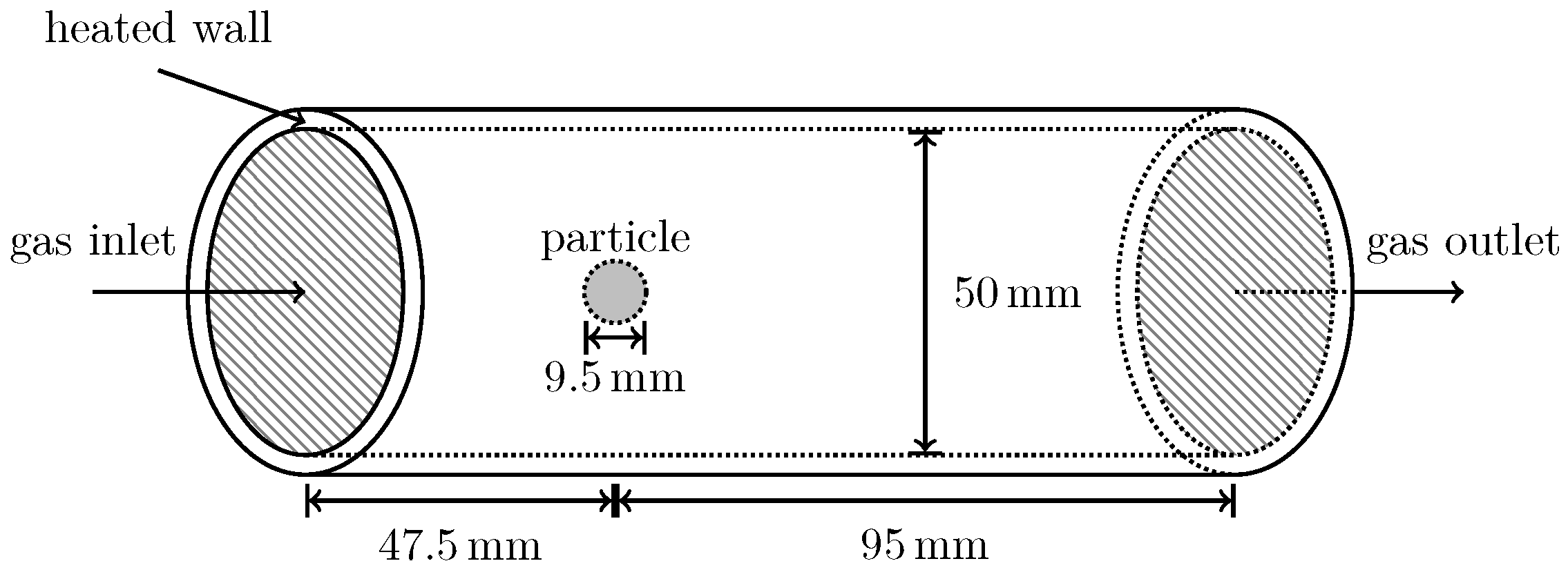
The validation for the use of the RLPM over 0D Lagrangian particle models in OF is presented here. The validation uses the experimentally obtained mass loss curves of biomass decomposition data by Lu et al. [23]. In these experiments spherical poplar wood particles with diameters of $9.5$ $\mathrm{m}$$\mathrm{m}$ are thermochemically converted under varying conditions. Three cases are considered: pyrolysis of dry wood, pyrolysis of wet wood (both under N₂ atmosphere), and the combustion of wood (under air atmosphere).

The occurring intra-particle gradients were the main reason for choosing Lu et al.’s [23] experimental data for the validation, even though the particles are up to three orders of magnitude larger. In addition, we are not aware of any similar experimental data for µm-sized particles.

Figure 1 shows the simulation setup. The particle properties for the validation and the RW experiments in the following section are identical (except for varying moisture content for this validation) and listed in Table 1. The simulation conditions for the different validation cases are listed in

Table 6. Energy and momentum BC and initial conditions for the validation cases.

Patch	Temperature	Pressure	Velocity
inlet	1050 [K]	$\nabla p=0$ [Pa/m]	3 [m/s]
outlet	$\nabla T=0$ [K/m]	$1·{10}^5$ [Pa]	$\nabla U=0$ [1/s]
walls	1276 [K]	$\nabla p=0$ [Pa/m]	3 [m/s]

and

Table 7. Initial mass fractions for the three validation cases for particle moisture content based on wet mass (w.b.), and surrounding gas phase. Gas phase mass fractions are set as fixed values for the inlet and wall BCs and as initial conditions in the simulation domain.

	Moisture [kg/kg] w.b.	N2 [kg/kg]	O2 [kg/kg]	H2O [kg/kg]
dry pyrolysis	0.06	1	0	0
wet pyrolysis	0.4	1	0	0
combustion	0.4	0.766	0.23	0.004

. The homogeneous gas phase reactions for the validation case are listed in

Table 8. Homogeneous carrier phase reactions, their pre-exponential factors A, and activation energies $E_a$.

	Homogeneous Reaction	A [kmol, m, K, s, J]	${\mathbf{E}}_{\mathbf{a}}$ [J/kmol]	Ref.
R8	${\mathrm{CH}}_4+1.5{\mathrm{O}}_2\to \mathrm{CO}+2{\mathrm{H}}_2\mathrm{O}$	$5.03·{10}^{11}$	$2·{10}^8$	[44]
R9	$\mathrm{CO}+{\displaystyle \frac{1}{2}}{\mathrm{O}}_2\to {\mathrm{CO}}_2$	$2.24·{10}^{12}$	$1.67·{10}^8$	[44]
R10	${\mathrm{CO}}_2\to \mathrm{CO}+{\displaystyle \frac{1}{2}}\mathrm{O}2$	$5·{10}^8$	$1.7·{10}^8$	[44]
R11	$\mathrm{CO}+\mathrm{CO}+{\mathrm{H}}_2\mathrm{O}\to {\mathrm{CO}}_2+{\mathrm{H}}_2$	$2.75·{10}^9$	$8.37·{10}^7$	[45]
R12	${\mathrm{CO}}_2+{\mathrm{H}}_2\to \mathrm{CO}+{\mathrm{H}}_2\mathrm{O}$	$9.98·{10}^{10}$	$1.21·{10}^8$	[45]

.

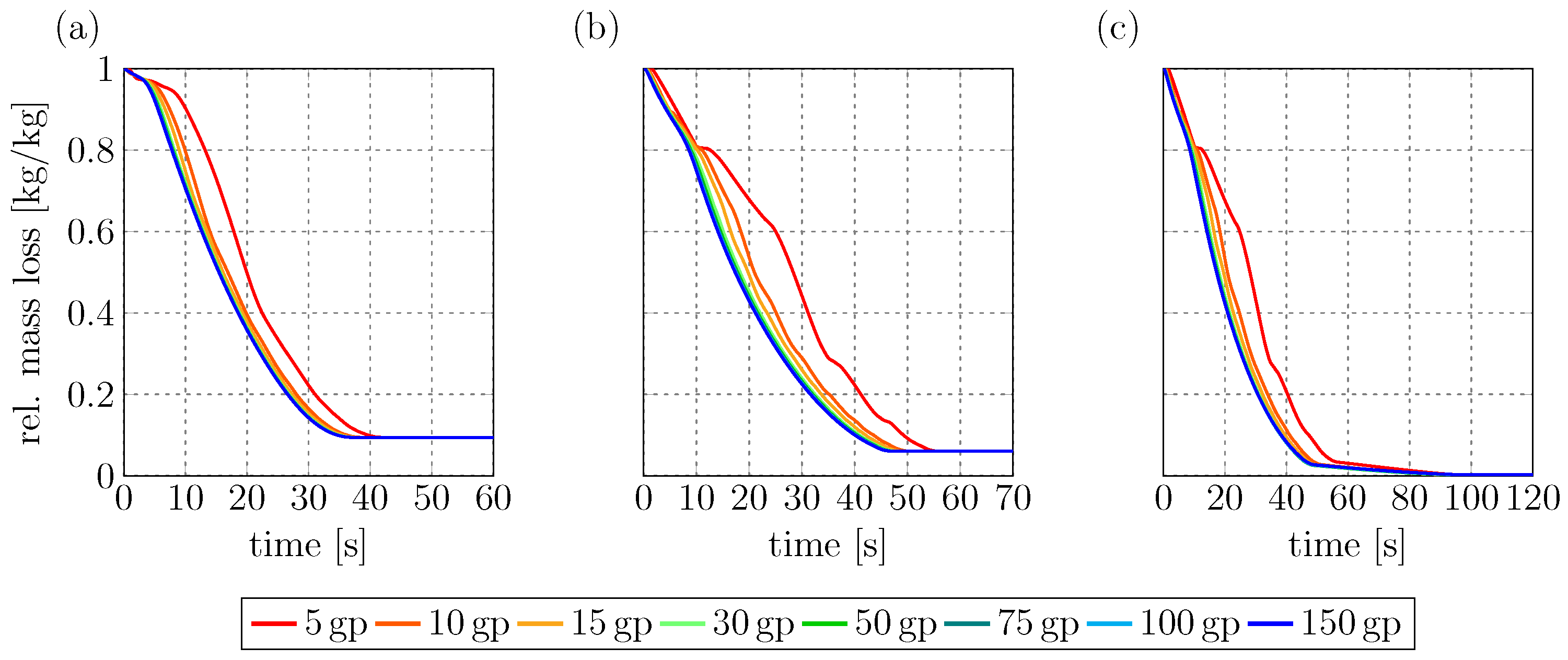
The first point in the validation is to establish the internal particle resolution needed for grid-independent results.

Figure 2 shows the mass loss curves obtained via the RLPM for all three experimental conditions. Under all three simulation conditions, the results converge to the same curve once the internal resolution is above 50 grid points. To assure results that are independent of the internal particle resolution, 100 internal grid points were chosen for the simulations in the next section.

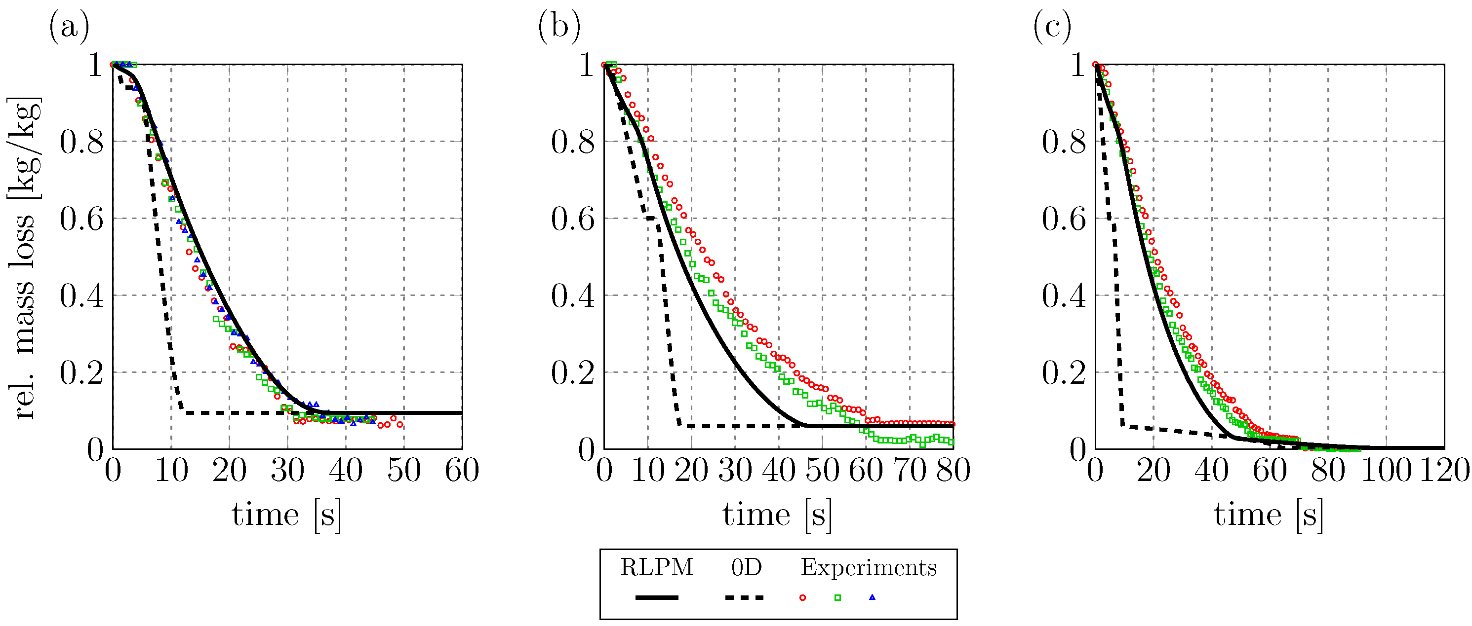
Figure 3 shows the mass loss curves of the RLPM compared to a 0D benchmark model and the experimental data by Lu et al. The benchmark model is described in [9,46] and uses the same reaction kinetics as the RLPM for this study (see Table 3 and Table 5).

The mass loss predictions of the RLPM are much closer to the experimental results than those of the 0D benchmark model. This shows the advantage of resolving internal gradients for thermally thick particles. However, the RLPM predictions are better for the dry case than for the wet case and the combustion case. This deviation at high moisture contents can be explained by the missing convective fluxes in Equations (4) and (6). Especially for high moisture contents, the gas release inside the particle leads to a pressure increase that forces an advective flow to the particle surface. This simplification was made to decrease the numerical complexity of the model and to allow for larger numbers of particles to be simulated. Despite this simplification, the RLPM shows reasonable mass loss predictions in all three cases shown in Figure 3.

In the following sections the focus is on the prediction of conversion times for (potentially) thermally thick particles. Therefore, the RLPM seems to be better suited than the 0D model.

5. Blast Furnace Raceway Zone Modeling

Figure 4 shows a schematic depiction of a typical BF used to convert iron ore to pig iron. The RW is the cavity that is created by the injection of hot blast and reducing agents (e.g., pulverized coal or biomass) from the tuyere into the active coke zone. The reducing agents need to be fully converted inside the RW for efficiency. Otherwise, the reducing agents can be transported toward the dead man and the BF stack, leading to clogging and a decreased BF efficiency. Biomass as an alternative reducing agent might lead to incomplete conversion inside the RW because it can have larger particle sizes compared to pulverized coal due to differing grinding properties.

The Eulerian part of the RW CFD simulation is based on the 3D RW obtained by Wartha et al. [10] using the RW model described in [9,46] and using pulverized coal as reducing agent. The complete converged RW CFD simulation results produced by Wartha et al. in OF were available and used for the current study. The simulation describes a $3.5$ $\mathrm{m}$ high, axially symmetric wedge of the blast furnace.

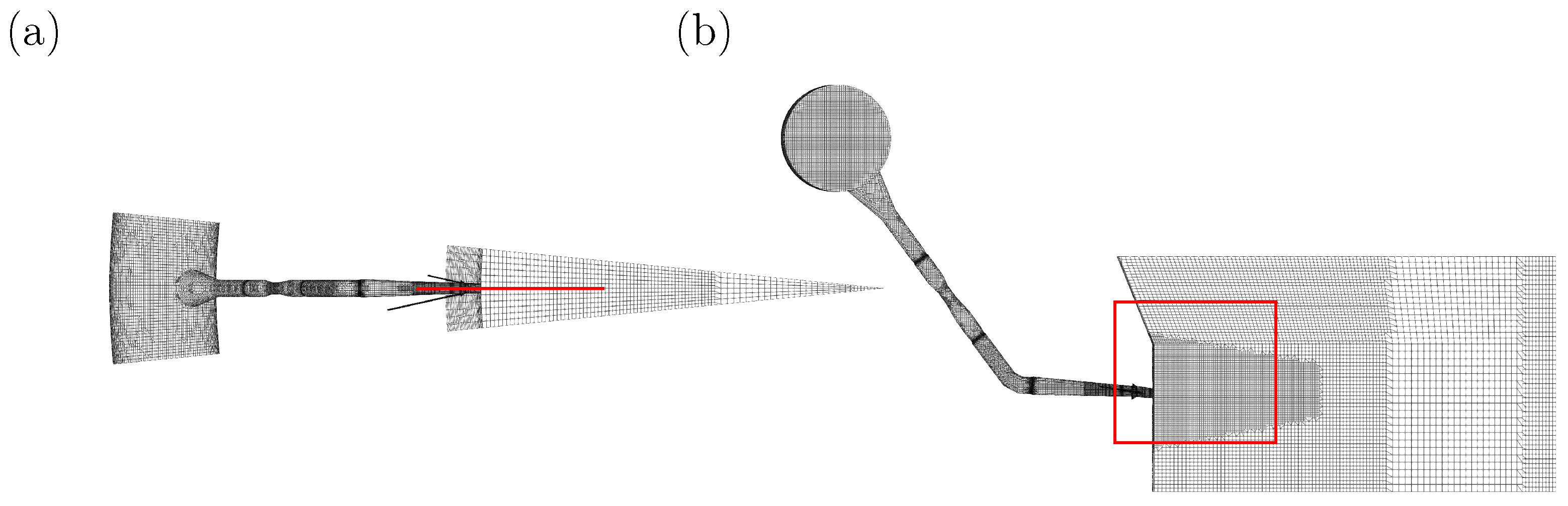
Figure 5 shows the simulation domain from above (a) and from the side (b). The position of the symmetry plane used to visualize the RW conditions and the particle trajectories in the following is indicated in Figure 5a as a line, and Figure 5b as a rectangle. The mesh is hexa-dominant and consists of over 300,000 cells. The validation results for this simulation framework of the RW are presented in [47].

The RW simulation assumes two Eulerian phases for gaseous blast and for solid coke. The coke phase is assumed to be stationary with a pre-set porosity profile that defines the cavity that forms the RW [10]. The bottom of the simulation domain is considered to be impenetrable by the hot blast. The top of the simulation is an outlet for the blast. Pulverized coal is injected into the RW through the tuyere. The RW conditions presented here were achieved by injecting 680 $\mathrm{k}\mathrm{g}$/h⁻¹ in the form of 2000 parcels per second [10].

The coke conversion in the RW is modeled using oxidation and CO₂ conversion, as well as H₂O conversion. The pulverized coal conversion uses an unresolved 0D Lagrangian particle model and an effectiveness factor approach to model oxidation, CO₂ gasification, and H₂O gasification, as well as an additional competing two-step mechanism for devolatilization. The homogeneous gas phase chemistry includes a modified R8 for volatiles and R9+R10 from Table 8. The detailed reaction mechanism can be found in [10].

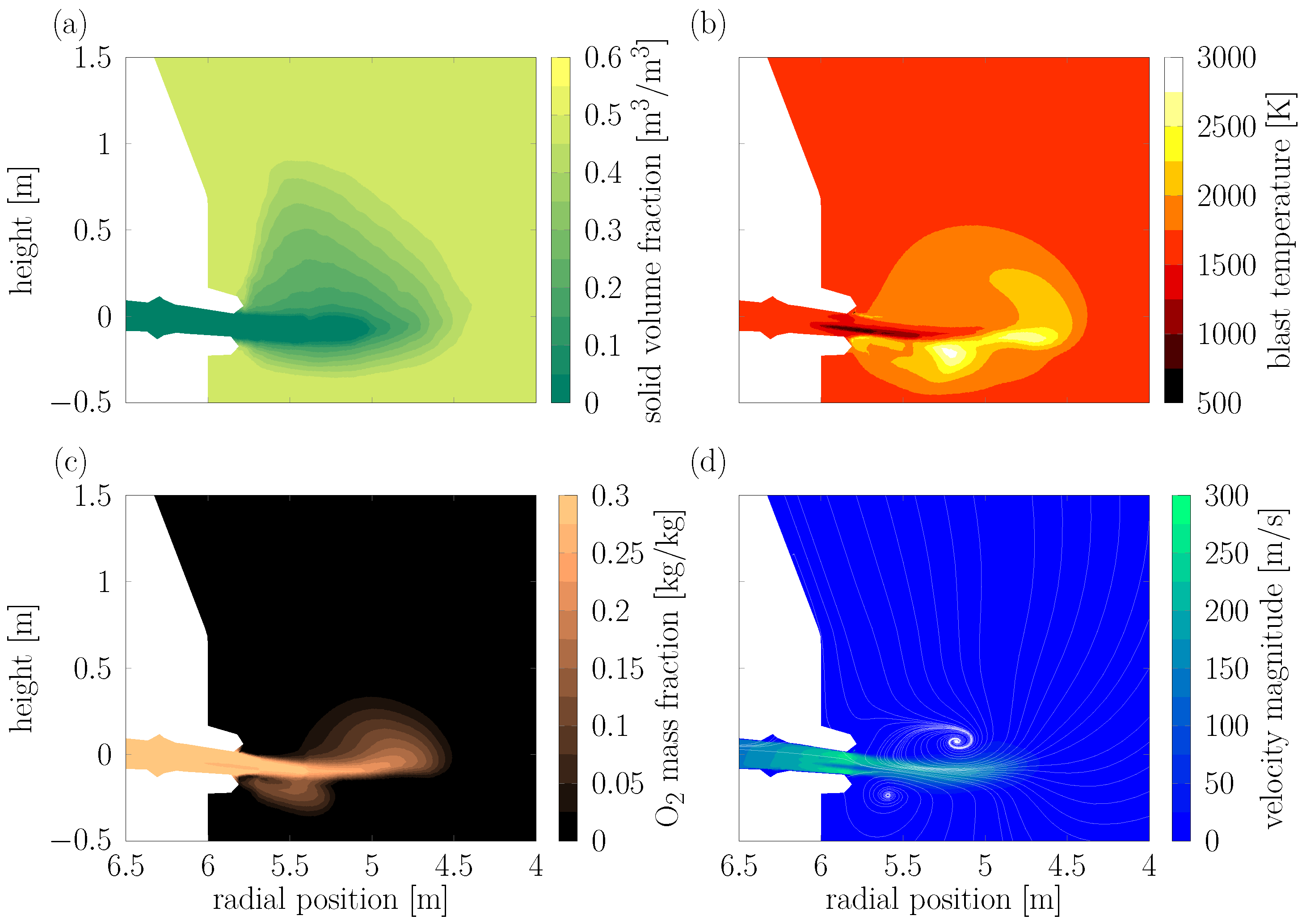
Figure 6 shows a cut through the RW zone CFD simulations in radial direction, along the plane the particles are injected into. The particles are removed when they encounter a solid mass fraction, ${\alpha }_{solid}$ equal to 0.5 inside the RW (Figure 6a). The particles are injected through a lance in the tuyere on the left side of the RW with an initial velocity of 15 m/s. The particles are injected into the 0.0093 Nm³/h hot blast stream, which contains 30% O₂ and 70% N₂. The oxygen concentration inside the RW is shown in Figure 6b. The blast temperature is shown in Figure 6c. The initial blast temperature at the inlet of the tuyere on the left is set to 1523 K, while the bottom of the simulation domain is set to a fixed value of 1673 K. Inside the RW, the particles experience blast temperatures of up to 2500 K and a non-uniform flow field with vortices branching off to the top and bottom of the RW and gas velocities of over 250 m/s (Figure 6d). For further details on the RW CFD simulation, the reader is referred to [10], as only the converged results are used in the study of biomass in the next section.

6. Simulation Results

Based on the approach from [7] biomass particles with 9 different diameters (50 $\mathsf{\mu }$$\mathrm{m}$, 75 $\mathsf{\mu }$$\mathrm{m}$, 100 $\mathsf{\mu }$$\mathrm{m}$, 150 $\mathsf{\mu }$$\mathrm{m}$, 200 $\mathsf{\mu }$$\mathrm{m}$, 250 $\mathsf{\mu }$$\mathrm{m}$, 300 $\mathsf{\mu }$$\mathrm{m}$, 350 $\mathsf{\mu }$$\mathrm{m}$, 500 $\mathsf{\mu }$$\mathrm{m}$) were chosen for the following study of their conversion behavior. For each diameter 1000 particles were injected to allow for a statistical analysis of their behavior. The RLPM parameters used to model the properties of biomass are listed in Section 3, Table 1, Table 2, Table 3, Table 4 and Table 5, with 100 internal grid points. Particles are typically dried before being injected into the RW of the BF, which leads to the relatively low moisture content of 8% listed in Table 1. The low moisture content and expected internal gradients for the larger particle diameters are the reasons for the choice of validation experiment in Section 4. In the validation the RLPM showed the best results for the dry pyrolysis case.

In real world applications biomass would be injected together with pulverized coal into the BF. However, the amount of pulverized coal that is injected would be orders of magnitude larger than the amount of biomass that is co-injected. Therefore, the converged RW zone CFD results that were obtained by Wartha et al. [10] by injecting pulverized coal into the RW (see Section 5) will be used to determine the biomass conversion. The biomass is only injected on top of the obtained flow field, without taking into account two-way coupling. This works under the assumption that the RW formation is dominated by the injection of pulverized coal, and the amount of injected biomass is not enough to significantly change the shape of the RW. However, clogging can still be an issue outside the RW if unconverted biomass exits the RW zone. This approach allows us to investigate biomass conversion under the same RW conditions as pulverized coal, leading to a better quantitative comparison.

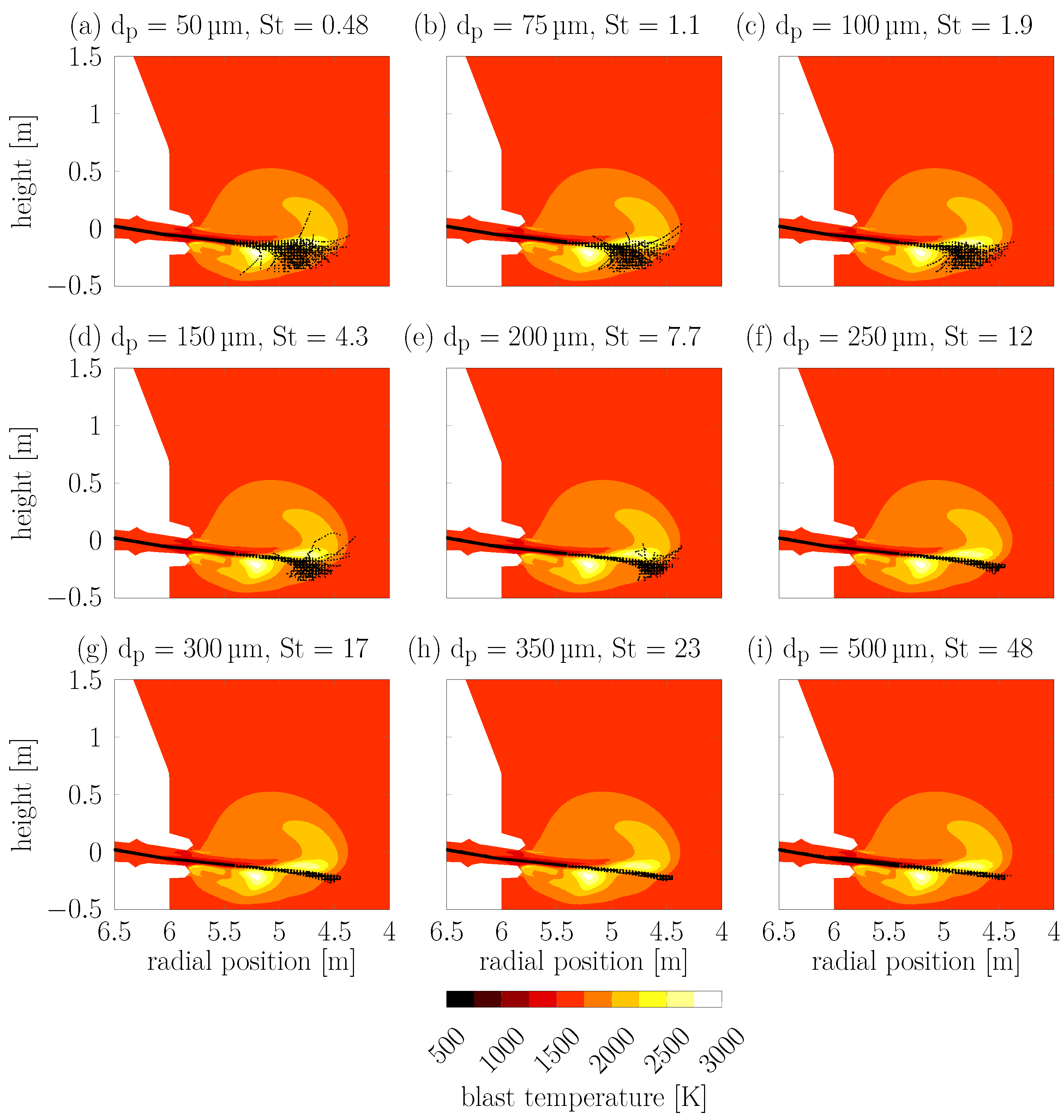
Figure 7 shows the individual particle trajectories of all 1000 particles for each of the different particle diameters on top of the RW blast temperature, as well as the associated Stokes numbers ($St$) for each diameter at the moment of injection.

The smaller particles with $St$ below 10 ($d_p\le 200\mathsf{\mu }\mathrm{m}$) follow the fluid flow more closely and the individual trajectories show a larger spread. The larger particles ($d_p\ge 250\mathsf{\mu }\mathrm{m}$) have almost complete uniform trajectories that only sample a narrow line through the RW. This means that only the particles with $St<10$ travel through the zones of highest blast temperature seen in Figure 7.

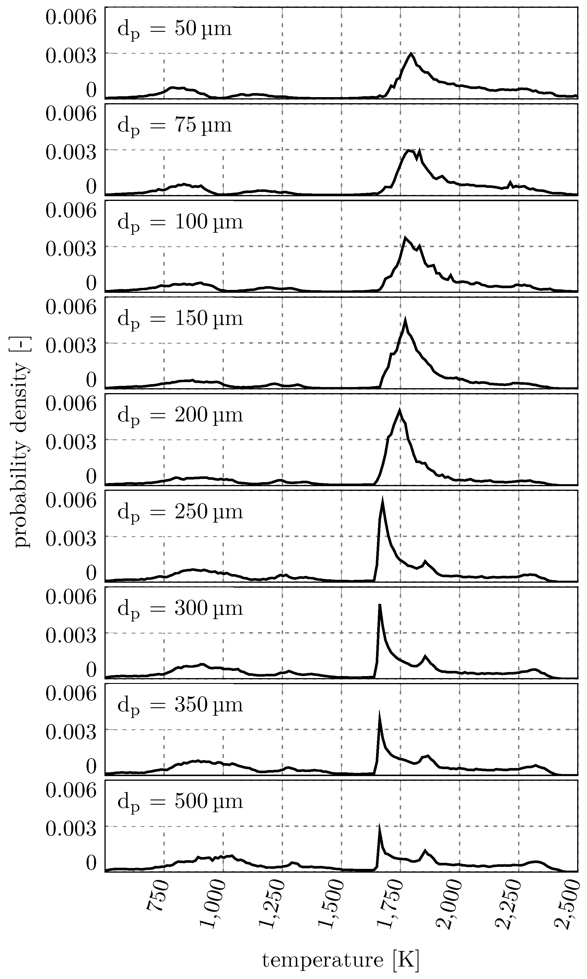
This behavior is quantified in Figure 8, where all particle trajectories in the RW were sampled in 0.01 ms time steps and then the probability density of encountering certain temperatures is derived from the resulting histogram. This allows for an understanding of how often different carrier phase temperatures are encountered by the particles inside the RW.

The most interesting region in the temperature distribution is the region between 1600 K and 2500 K. This region shows the most common temperatures the particles encounter, which influences their conversion degree. The most common temperature that is encountered by the particles decreases with increasing diameter. The smaller particles with $St<10$ (diameters < 250 $\mathsf{\mu }$$\mathrm{m}$) have peaks at or above 1750 K. The larger particles are more likely to encounter lower temperatures and the peak is at 1650 K. Due to the similar trajectories of the larger particles (diameters ≥ 250 $\mathsf{\mu }$$\mathrm{m}$) these particles encounter very similar temperatures. The effect that smaller particles travel through regions of higher temperature in combination with the larger specific surface area lead to an even faster conversion of the small particles compared to the larger particles.

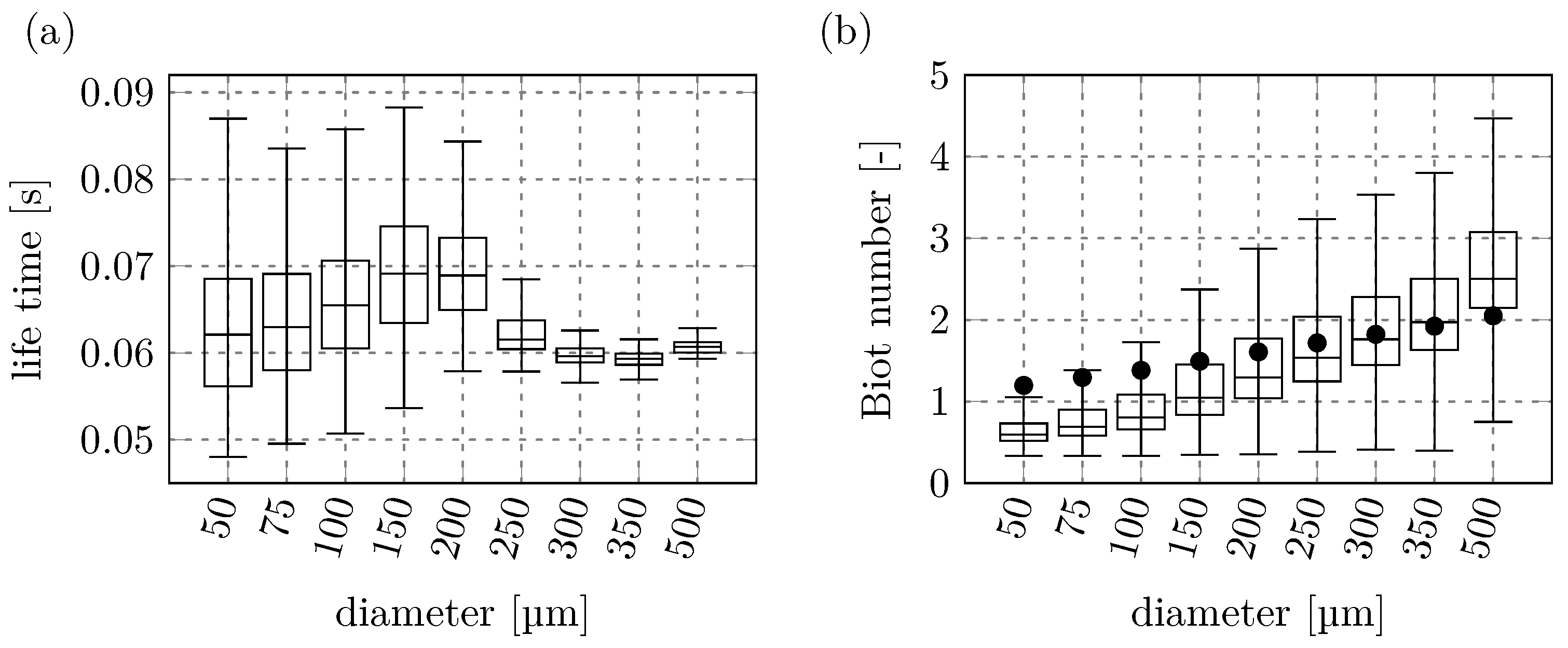
Figure 9a shows how much time the particles of each diameter spent inside the RW, from the time of insertion to the time of removal. The median lifetime of all particles is within a 10 ms window between 60 ms and 70 ms. Particles with diameters of $d_p\le 200\mathsf{\mu }\mathrm{m}$ show an increasing lifetime with increasing diameter, then there is a drop in the median lifetime for the larger particles with $d_p\ge 250\mathsf{\mu }\mathrm{m}$ and the lifetimes stay almost constant. Generally, the particle velocity decreases with increasing diameter. However, the particles with $d_p\ge 250\mathsf{\mu }\mathrm{m}$ have much straighter trajectories through the RW, leading to shorter residence times before exiting the RW. This means that the largest four particle diameters have less time for the thermochemical conversion inside the RW, which further reduces their final conversion rates.

In Figure 9b the Biot number ($Bi$) distribution for each particle diameter is shown. The black dot in the box plot represents the Biot number that was calculated using the initial conditions around the particle at the point of injection. The figure shows that the Biot number estimated for the particles at injection is not necessarily representative of the median Biot number of the particles inside the RW zone. For small particles the initial Biot number is overestimated, and for larger particles, it is underestimated. All particles can be seen to be in the thermally thick regime ($Bi>0.1$ [48]). However, the smallest radii show Biot numbers consistently below 1, which results in only small internal temperature gradients when compared to the larger particles. Larger temperature gradients for larger particles lead to an increase in the variation around the median value of the Biot numbers seen in Figure 9b with increasing particle diameters.

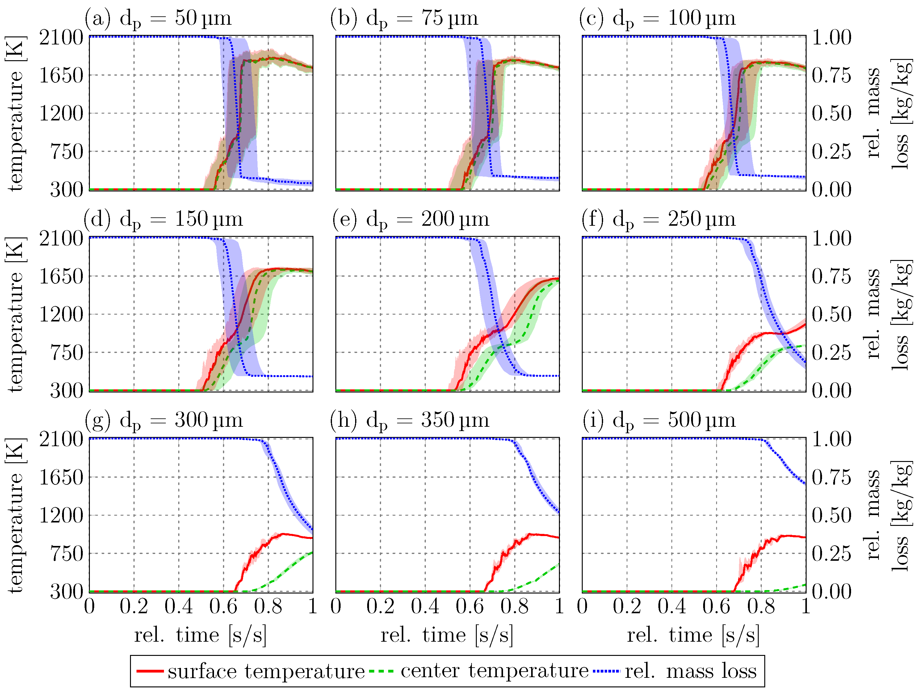
Figure 10 shows the median surface and center temperatures, as well as the mass loss over the normalized lifetime for all nine diameters. Figure 10 also includes the 25% and 75% quantiles to show deviation from the median. The deviation from the median value is larger for the particles with $St<10$ ($d_p\le 200\mathsf{\mu }\mathrm{m}$), and smaller for the particles with $St>10$ ($d_p\ge 250\mathsf{\mu }\mathrm{m}$).

This is in line with Figure 7 and Figure 8, where the smaller particles sample more diverse paths through the RW, leading to larger differences between the individual particles. Up to particle diameters of 200 $\mathsf{\mu }$$\mathrm{m}$, the median particle surface temperatures reach a maximum of approximately 1600 K to 1800 K, the center temperatures are only slightly smaller than the surface temperatures, and the particles are almost isothermal. In general, these particles have enough time in the RW zone for (almost) complete thermochemical conversion, as can be seen in the median mass loss curve. For particle diameters of 250 $\mathsf{\mu }$$\mathrm{m}$ and above, the particle center does not heat up to the same temperature as the particle surface. The maximum surface temperature for these particles is between 900 K and 1100 K, while the maximum center temperatures are between 400 K and 800 K. These particles mostly show non-isothermal behavior and do not spend enough time in the RW for complete heat-up. However, the temperatures at the particle surface are sufficient for pyrolysis, leading to relative mass losses between 80% for 250 $\mathsf{\mu }$$\mathrm{m}$ particles and 30% for 500 $\mathsf{\mu }$$\mathrm{m}$ particles.

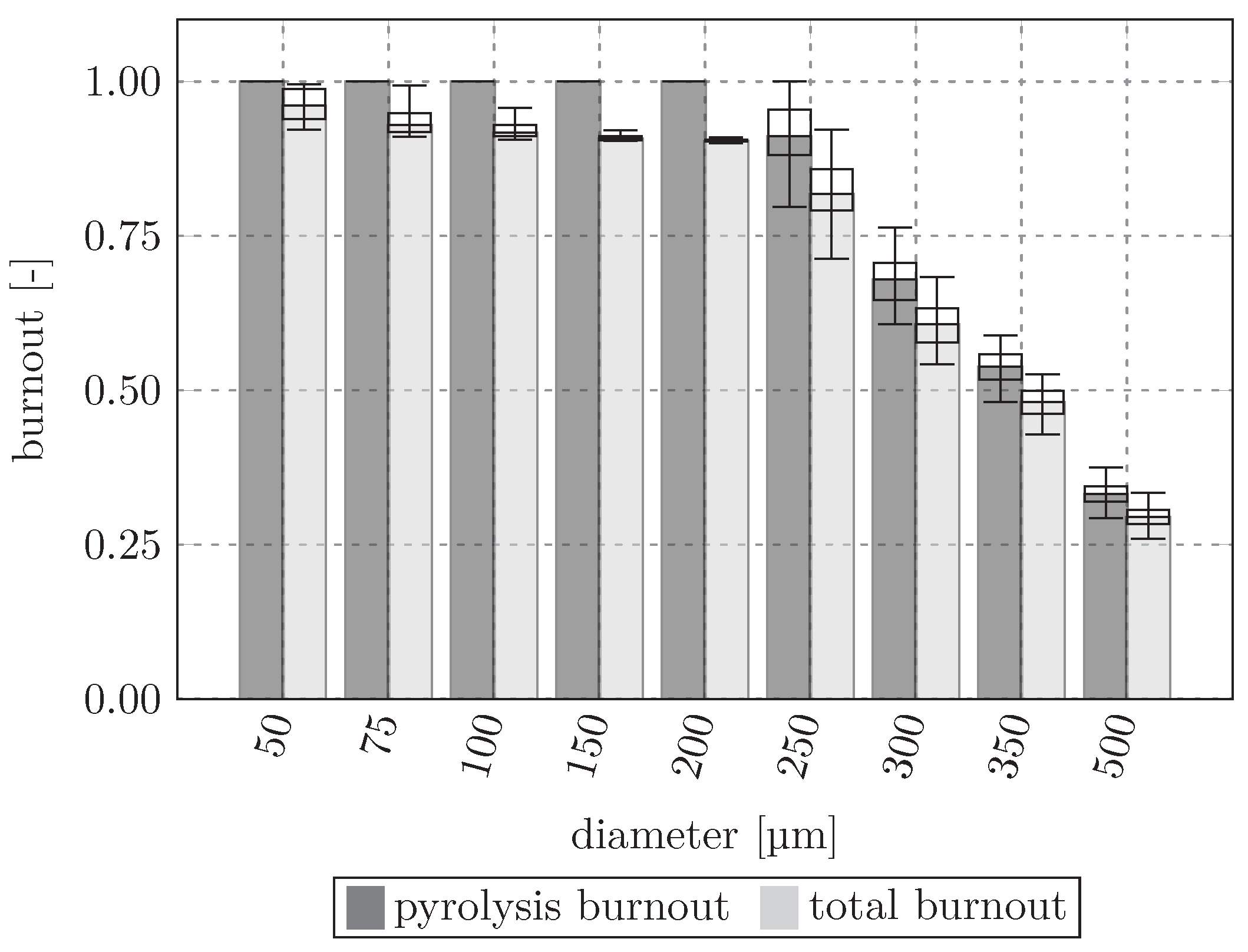
Figure 11 shows the pyrolysis burnout and total burnout at the end of the particle lifetime. The particle mass is initially completely composed of biomass in the form of cellulose, hemicellulose, and lignin, which each decompose into the gas and solid components listed in Table 4. The pyrolysis burnout describes the relative amount of biomass that was converted compared to the initial particle mass, while the total burnout also takes char conversion into account. Up to $d_p=200\mathsf{\mu }\mathrm{m}$ the biomass is fully decomposed, and a part of the produced char is also converted. However, starting at $d_p=250\mathsf{\mu }\mathrm{m}$ the average particle composition still contains unconverted biomass. At the largest diameter ($d_p=500\mathsf{\mu }\mathrm{m}$) only around 30% of the biomass has been converted by the time the particles exit the RW zone. Therefore, particles from 250 $\mathsf{\mu }$$\mathrm{m}$ and above will transport increasing amounts of biomass toward the dead man and BF stack. In general, particles should be converted as completely as possible inside the RW in order to increase the BF efficiency and decrease the resource consumption. Only the particles with $d_p\le 200\mathsf{\mu }\mathrm{m}$ show median conversion rates of over 90%.

7. Conclusions

The RLPM, a 1D, internally resolved Lagrangian particle model, was employed to assess the suitability of biomass particles with different diameters as ARAs in the RW. Particles with diameters ranging from 50 $\mathsf{\mu }$$\mathrm{m}$ to 500 $\mathsf{\mu }$$\mathrm{m}$ were injected into the frozen flow field of a BF RW. The median Biot number for all particles is above 0.1, which means all particles are thermally thick and, therefore, the use of the resolved 1D Lagrangian particle model is required.

Only particles with diameters below 250 $\mathsf{\mu }$$\mathrm{m}$ fully pyrolyze and partially convert the remaining char before exiting the RW. The particles with diameters of 250 $\mathsf{\mu }$$\mathrm{m}$ and above spend less time inside the RW than smaller particles, because they have straight trajectories through the RW, while smaller particles’ trajectories are diverted by the non-uniform flow field. As a consequence, the larger particles’ trajectories miss the regions with the highest temperatures in the RW, leading to lower heating rates.

The results of the performed simulations thus show that only biomass particles below 250 $\mathsf{\mu }$$\mathrm{m}$ were suitable for use as alternative reducing agents in the RW of the BF.

In the current work a fully converged RW CFD simulation with a frozen RW shape was employed, using only pulverized coal as reducing agent [10]. Due to the small size ( 2 $\mathsf{\mu }$$\mathrm{m}$ to 100 $\mathsf{\mu }$$\mathrm{m}$) and resulting low Stokes numbers of pulverized coal, the regions of highest temperatures are not directly in the injection axis but above and below it, where the vortices in the flow field transport smaller particles and they subsequently thermochemically convert. The biomass particles are then injected on top of the fully converged RW CFD flow and temperature fields with one-way coupling. This means that the biomass has no influence on the Eulerian fields of the simulation. This is justified by the assumption that biomass would only be added in small quantities to the pulverized coal that is injected into the RW and, therefore, has only a small effect on the RW itself. However, despite the biomass being added in a small quantity to the injected pulverized coal, the BF is still sensitive to clogging due to unreacted particles exiting the RW. Furthermore, the aim of this study was to investigate biomass conversion behavior under known RW conditions, allowing for a better comparison with pulverized coal as a reducing agent, rather than investigating the change of the RW state.

The two main points to improve the simulations are to add two-way coupling for the biomass particles and to inject both biomass and pulverized coal together, as well as to allow for a dynamic RW shape. This approach could slightly alter the Eulerian fields. However, the computational effort would be much higher in this case, considering that the RLPM is more computationally expensive than the 0D model used for modeling pulverized coal. Additionally, a dynamic RW is also less numerically stable and further adds to the computational cost. At the moment this is prohibitive; however, work is ongoing to optimize the simulation methods used in OpenFOAM^® and to make these simulations feasible in the future.

The current results and approach can be used for further studies that focus on evaluating different injection velocities and angles for biomass particles. Adjusting these parameters may extend particle residence time and redirect larger particles toward higher-temperature regions within the raceway, potentially enhancing their conversion rates and making them more viable as ARAs, for particle diameters above 250 $\mathsf{\mu }$$\mathrm{m}$.