Factors Impacting Projected Annual Energy Production from Offshore Wind Farms on the US East and West Coasts

Abstract

Simulations are conducted using a microscale model framework to quantify differences in projected Annual Energy Production (AEP), Capacity Factor (CF) and wake losses for large offshore wind farms that arise due to different input datasets, installed capacity density (ICD) and/or wake parameterizations. Differences in CF (and AEP) and wake losses that arise due to the selection of the wake parameterization have the same magnitude as varying the ICD within the likely range of 2–9 MW km⁻². CF simulated with most wake parameterizations have a near-linear relationship with ICD in this range, and the slope of the dependency on ICD is similar to that in mesoscale simulations with the Weather Research and Forecasting (WRF) model. Microscale simulations show that remotely generated wakes can double AEP losses in individual lease areas (LA) within a large LA cluster. Finally, simulations with the Coupled Ocean-Atmosphere-Wave-Sediment Transport (COAWST) model are shown to differ in terms of wake-induced AEP reduction from those with the WRF model by up to 5%, but this difference is smaller than differences in CF caused by the wind farm parameterization used in the mesoscale modeling. Enhanced evaluation of mesoscale and microscale wake parameterizations against observations of climatological representative AEP and time-varying power production from wind farm Supervisory Control and Data Acquisition (SCADA) data remains critical to improving the accuracy of predictive AEP modeling for large offshore wind farms.

1. Introduction

Approximately 8 GW of offshore wind energy capacity was installed in 2024 bringing the global total to 83 GW [1], around half of which is in China [2]. While this remains a small fraction of total global wind energy installed capacity (IC) (1.136 TW at the end of 2024), plans to install over 150 GW of offshore wind energy are in place for the next six years [1] including 51 GW additional to the existing 35 GW of capacity in the European Union [3]. Planned developments are likely to fall short of the 380 GW of offshore wind required by 2030 to reach the 1.5 °C climate goal [4]. Nonetheless, these ambitious targets require thousands of offshore wind turbines and their associated infrastructure to be deployed.

The IC for individual offshore wind farms in Europe almost doubled in the decade ending 2019 to 621 MW [5] and remained slightly over 600 MW for new installations in 2024 [6]. As these offshore wind farms are developed in areas with short distance to the coastline, major markets and low water depth, they are increasingly being developed in close proximity to each other [7]. Hence, most wind turbines operate in waked conditions (downwind of other wind turbines) for most of the time. Power losses due to wakes are an important component of the Levelized Cost of Energy (LCoE) because they reduce Annual Energy Production (AEP) [8]:

$$\mathrm{L}\mathrm{C}\mathrm{o}\mathrm{E}={\displaystyle \frac{\mathrm{C}\mathrm{A}\mathrm{P}\mathrm{E}\mathrm{X}\times \mathrm{C}\mathrm{R}\mathrm{F}+\mathrm{O}\mathrm{P}\mathrm{E}\mathrm{X}}{\mathrm{A}\mathrm{E}\mathrm{P}}}$$

(1)

where CAPEX is the capital expenditure, CRF is the Cost Recovery Factor or fixed charge rate and OPEX are Operating Expenditures.

Capacity Factor (CF) is the ratio of the actual power production (usually over one year in which case Annual Energy Production (AEP) is used in its calculation) to the power production that would be generated if a wind turbine or wind farm ran at its rated capacity (R) for the whole time period. CF thus encompass the site-specific wind resource relative to the turbine power curve, and other losses including wakes and any non-operational times for wind turbines:

$$\mathrm{C}\mathrm{F}={\displaystyle \frac{\mathrm{A}\mathrm{E}\mathrm{P}}{\mathrm{R}\mathrm{n}}}$$

(2)

where n is the number of hours in a year.

The impact of power losses due to wakes on LCoE can be illustrated with a simple example. Disregarding CRF, assuming an offshore wind turbine has a rated capacity of 15 MW, CAPEX of $5 million, OPEX of 10% of CAPEX and a CF of 50% then LCoE is ~$84 MWh. If AEP is reduced by 10% due to wake losses, LCoE increases to $93 MWh and if wake losses are 30% LCoE increases to $120 MWh.

There are a number of logistical and technical challenges facing the offshore wind energy industry that also impact LCoE [1] including the complexity of planning procedures [7], the need for specialist ships and port infrastructure [9], environmental and other social constraints [10]. Over the last few years, unfavorable market conditions and continued downward pressure on the price for offshore wind-generated electricity has impacted developments [11]. In the 2023 auction, the UK government set a strike price of ₤44/MWh ($55/MWh) that failed to attract bids [12], as did two areas in the US Gulf of Mexico [13] and 3 GW offered by the Danish Government failed in 2024 [14]. These unfilled bids are attributed to a number of factors including supply chain issues, market frameworks, low prices offered for electricity and relatively high risks for a small number of companies with offshore wind energy capabilities [1]. Despite this, offshore wind energy remains a cost-effective cornerstone of many government energy policies [1] and relaunched bids by the UK government for 9.6 GW with a price of ₤73/MWh were successful in 2024 [15]. China has 437 offshore wind projects totaling 247 GW in the pipeline [2]. Thus, the offshore wind energy market remains strong but continued effort to reduce costs and uncertainties is required.

Despite increasing cost of installation, and operation and maintenance offshore, the relatively high CF offshore (assumed to be above 45% in the North Sea [16] and modeled to be above 45% for the United States of America (US) east coast LA [17]) still mean that electricity can be produced economically by offshore wind farms. Given the scale and density of offshore wind farms in areas that are currently being developed [7], CF are also increasingly influenced by wind turbine wakes. Wake losses (W) are calculated as

$$\mathrm{W}={\displaystyle \frac{\left({\mathrm{A}\mathrm{E}\mathrm{P}}_{\mathrm{f}\mathrm{s}}-\mathrm{A}\mathrm{E}\mathrm{P}\right)}{{\mathrm{A}\mathrm{E}\mathrm{P}}_{\mathrm{f}\mathrm{s}}}}$$

(3)

where AEP_fs is the Annual Energy Production of the freestream wind turbine (or multiplied by the number of wind turbines in the wind farm). AEP is from an individual turbine or the whole wind farm accounting for wake losses. W is usually expressed as a percentage of AEP.

As discussed in detail below, wake losses from offshore tend to be larger than those from onshore wind farms mainly due to the lower prevailing turbulence [18]. While wakes are not the only source of power losses from on- or off-shore wind farms they tend to be largest losses and to have the largest uncertainty. For example, for the proposed floating wind farms at Humboldt and Morro Bay, for planning purposes assumed power production losses are 1.6% for environmental, 1.2% technical, 4.3% electrical and 5.0% availability with modeled wake losses of between 4 and 9% [19]. Vineyard Wind I is currently being built off the U.S. east coast (and is discussed in detail later in this paper) is expected to have a final IC of 800 MW and CF over 45% [20]. Based on the prevailing wind resource, in the absence of power losses, it could be expected to generate at least 3.15 TWh of electricity per year. It has been reported that “The 20-year average cost of the two long-term contracts is $84.23 per MWh in levelized nominal dollar terms” [21]. In this case, each 1% loss of AEP is equivalent to at least $2.66 million of lost annual revenue. Hence, accurate wake assessment is critical to wind farm economics [8].

Optimal spacing between wind turbines within a wind farm array is a balance between the cost of each turbine and the cabling between turbines, potential electricity production in a given wind climate and lost electricity production due to wind turbine wakes [8]. While turbine spacing at some operating offshore wind farms is as small as 3 rotor diameters (D), e.g., 2.4 D at Middelgrund [18] and 3.3–4.3 D Lillgrund [22], spacing in larger arrays is typically greater (6–10 D) to reduce wake losses and to limit loading due to added turbulence in wakes. Reported total wake losses in offshore wind farms are typically in the range of 11–28% of AEP but these are for much smaller offshore wind farms (with IC of <110 MW) than those currently in development or that are planned [8].

Although approximately 8.5 GW of floating wind energy is expected to be installed globally by 2030 [4], it comprises only a few percent of the expected developments of 224 GW and there is a continued emphasis on bottom-mounted wind turbines. Most new installations will focus on water depths of less than 70 m and distances within about 130 km of the shoreline, which are a major constraint on areas for development [7]. Accordingly, areas like the North Sea and the US east coast have planned developments that are relatively closely spaced both within and downwind of each wind farm [7,16]. Inter-farm wakes refer to wake losses within the wind farm (or array) and intra-farm means wake losses between wind farms. Downwind of offshore wind farms (cluster effects) decreases in wind speed are expected to extend over very large distances. Modeling shows large-scale offshore wind farm wakes extend well over 25 km [23] and over 50 km in stable atmospheric stratification [7], and this is confirmed by satellite [24,25] aircraft [26] and radar observations [27]. Wind farm arrays (groups of wind turbines operated over a contiguous area by one developer (or consortium)) and clusters (group of wind farms close together and potentially operated by different developers or different consortia) are thus highly likely to wake one another leading to suggestions that there may be a need to implement either controls to maximize system-wide electricity production [28] and/or policy measures such as trading rights to consume wind [29].

Models indicate that power losses from wakes in very large offshore wind farms (over 10 GW in continuous areas and impacted by other arrays) could be as much as 37% [30]. Modeling of intra-farm wakes in the German Bight show power losses of 13% [31], while inter-farm or cluster wakes amount to 2.5–4.3% power losses and wind resource changes due to climate effects 0.03–4.2% by the end of the century [32]. The extent of wakes (defined as velocity deficits of 5% relative to the freestream) is 2–3 times the footprint of the actual wind farm or cluster and so wakes are an important planning consideration [7]. The magnitude of wake losses is anticipated to be large, but the wide range of values generated by different models and compute platforms presents a significant challenge to accurate assessment of optimal layouts and projections of LCoE. The magnitude of inter-farm and intra-farm wake losses is critically dependent on the following:

(1)

The layout and spatial extent of the wind farms. Here we describe the turbine layout using the installed capacity density (ICD) (defined as total installed wind turbine rated capacity divided by total area) to allow for irregular array layouts. Most large European offshore wind farms have ICD of 4–10 MW km⁻² [16]. Previous work suggests that AEP of large wind farms in wind climates with non-unidirectional wind direction distributions is sensitive to ICD but not the precise alignment of wind turbine rows/columns [8].

(2)

The model used to describe the generation and expansion of wind turbine wakes.

(3)

The sources of the meteorological data used to drive the wake models including assumptions regarding vertical extrapolation (if any) of wind speeds to wind turbine hub-height. Unfortunately, there is low availability of high-quality, long-duration, observations at wind turbine relevant heights for many offshore areas that are currently under consideration for large-scale wind turbine deployments [33]. Thus, most wake analyses employ meteorological output from reanalysis products or mesoscale simulations.

This study aims to quantify the uncertainty in projected power production from large offshore wind farms that derives from the source of wind climates, wake parameterizations, and wind turbine spacing/ICD. Most planned US offshore wind farms are of an unprecedented scale in terms of footprint of adjacent LA and are still in construction, so there are no power production data with which to validate wake models. Hence our approach is to use available models. This can serve to inform where additional data collection efforts or model improvements are required.

2. Methodology

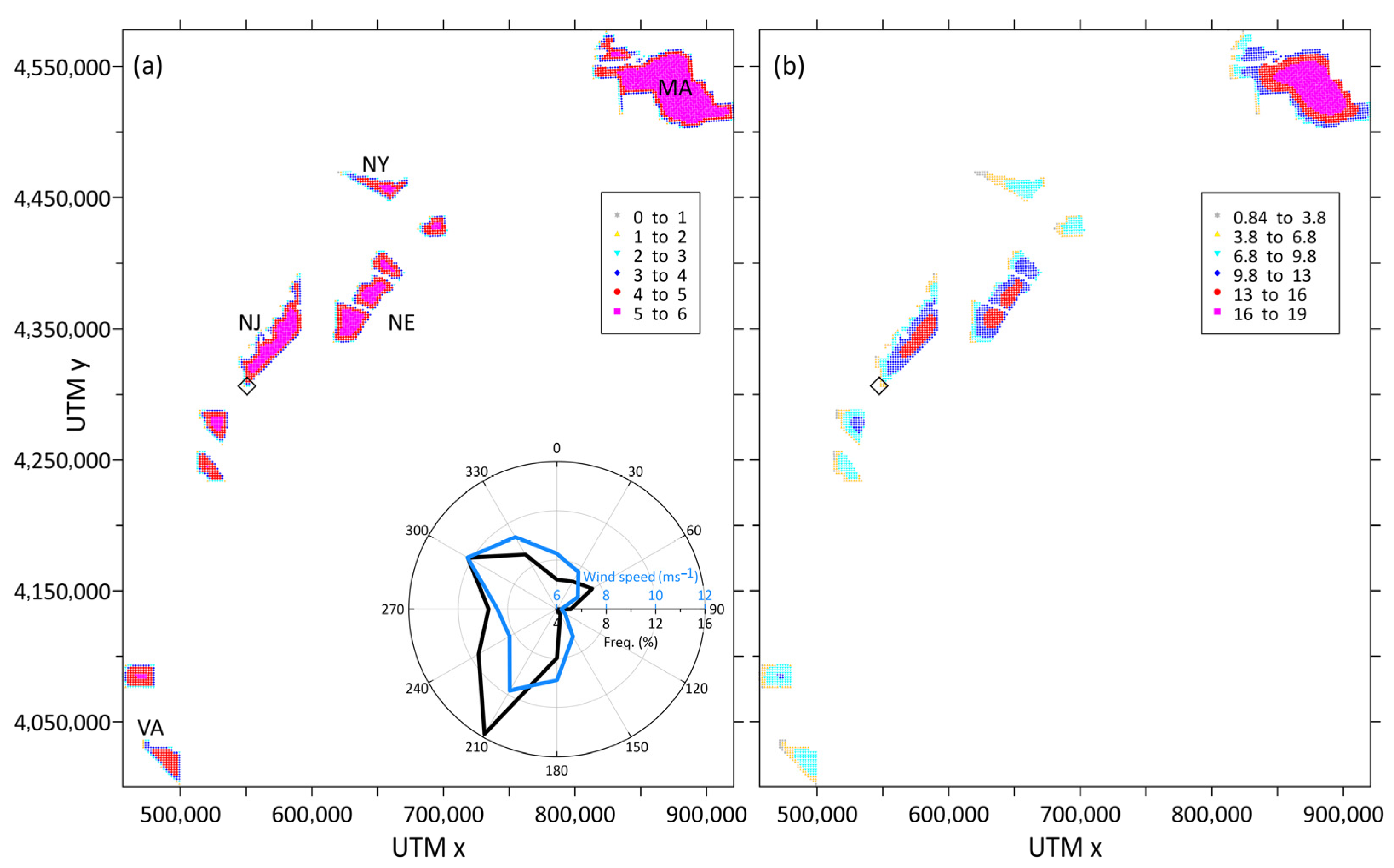
2.1. Offshore Wind Lease Areas

Offshore wind energy development is underway on the east and west coasts of the US. Offshore wind energy LA excluding those off Maine, North Carolina (NC) and the Gulf of Mexico [34] are shown in Figure 1. Initial modeling of the offshore wind power generation in this paper focuses on two areas—one encompasses the continuous group of LA to the south of the US states of Rhode Island (RI) and Massachusetts (MA) off the east coast (Figure 1a) while the second is Humboldt (HU, the more northerly of the LA shown in Figure 1b) off the west coast of California (CA). The major differences between the MA and HU LA are; (1) MA LA is nearly seven times the size (3673 km²) [8] of HU LA ~530 km² [19]; (2) water depth are less than 70 m in the MA LA (suitable for bottom-mounted turbines) and over 700 m at Humboldt [19] (suitable for floating turbines); (3) the wind resource at Humboldt is almost unidirectional (northerly) whereas the wind direction distribution at MA is omni-directional but dominated by southwesterly flow [35].

2.1.1. US East Coast

The 10 contiguous LA to the south of MA and RI cover almost 3670 km² (referred to herein using the abbreviation; MA LA) (Figure 1a). Here the entire MA LA cluster is modeled to examine the range of wake losses expected for very large wind farm clusters. Assuming full build out on a regular east–west grid with 1 nautical mile turbine spacing [36], MA LA (installed capacity (IC)~14 GW, 1071 turbines) will comprise rows and columns with more than 20 wind turbines and thus the potential for deep wake effects in most wind directions. It will be several times larger than the largest offshore wind farms currently being built in phases that is the 3.6 GW wind farm at Dogger Bank, UK [37].

A primary focus of the work presented here is the Vineyard I LA in the MA LA cluster which is the wind farm most advanced in terms of construction in US waters (February 2025) after completion of the South Fork (132 MW, 12 wind turbines) and Block Island (30 MW, five wind turbines) wind farms and two turbines at the Coastal Offshore Virgina project. The Vineyard I (VY) center is located at approximately ~41.0° N, 70.5° W and this LA covers ~306 km⁻² [20]. The closest distance to land is ~23 km from Martha’s Vineyard and Nantucket and water depths range between 35 and 60 m [35]. Sixty-two wind turbines will be installed. The wind turbines are 13 MW GE Haliade turbines with a nominal rotor diameter (D) of 220 m and hub-heights from 109 to 144 m. The resulting ICD is ~3 MW km⁻².

2.1.2. Humboldt LA

For the west coast, the Humboldt LA off the coast of California is selected here for analysis and has a central location of 41° N, 124.6° W (Figure 1b). It is 34 km from land at its closest point and covers an area of 536 km² with a projected IC of 1.6 GW, equivalent to an ICD of ~3 MW km⁻². The water depth at the Humboldt LA ranges from 500 to 1100 m and hence floating turbines will be employed [38].

Figure 1. Locations of all auctioned offshore wind energy lease areas (LA in red) (as of September 2024) along (a) the US east coast and (b) west coast. LA for which specific simulations are provided are highlighted in shades of blue. In panel (a) the MA LA cluster is shown in cyan with the Vineyard I LA highlighted in blue. In panel (b) the Humboldt LA is shown in blue. State abbreviations are given, and the maps are on the same scale to aid comparison. The inset figure in panel (a) shows the power (right axis in MW) and thrust (left axis) curves for the IEA 15 MW reference wind turbine that is used in all the simulations [39].

Figure 1. Locations of all auctioned offshore wind energy lease areas (LA in red) (as of September 2024) along (a) the US east coast and (b) west coast. LA for which specific simulations are provided are highlighted in shades of blue. In panel (a) the MA LA cluster is shown in cyan with the Vineyard I LA highlighted in blue. In panel (b) the Humboldt LA is shown in blue. State abbreviations are given, and the maps are on the same scale to aid comparison. The inset figure in panel (a) shows the power (right axis in MW) and thrust (left axis) curves for the IEA 15 MW reference wind turbine that is used in all the simulations [39].

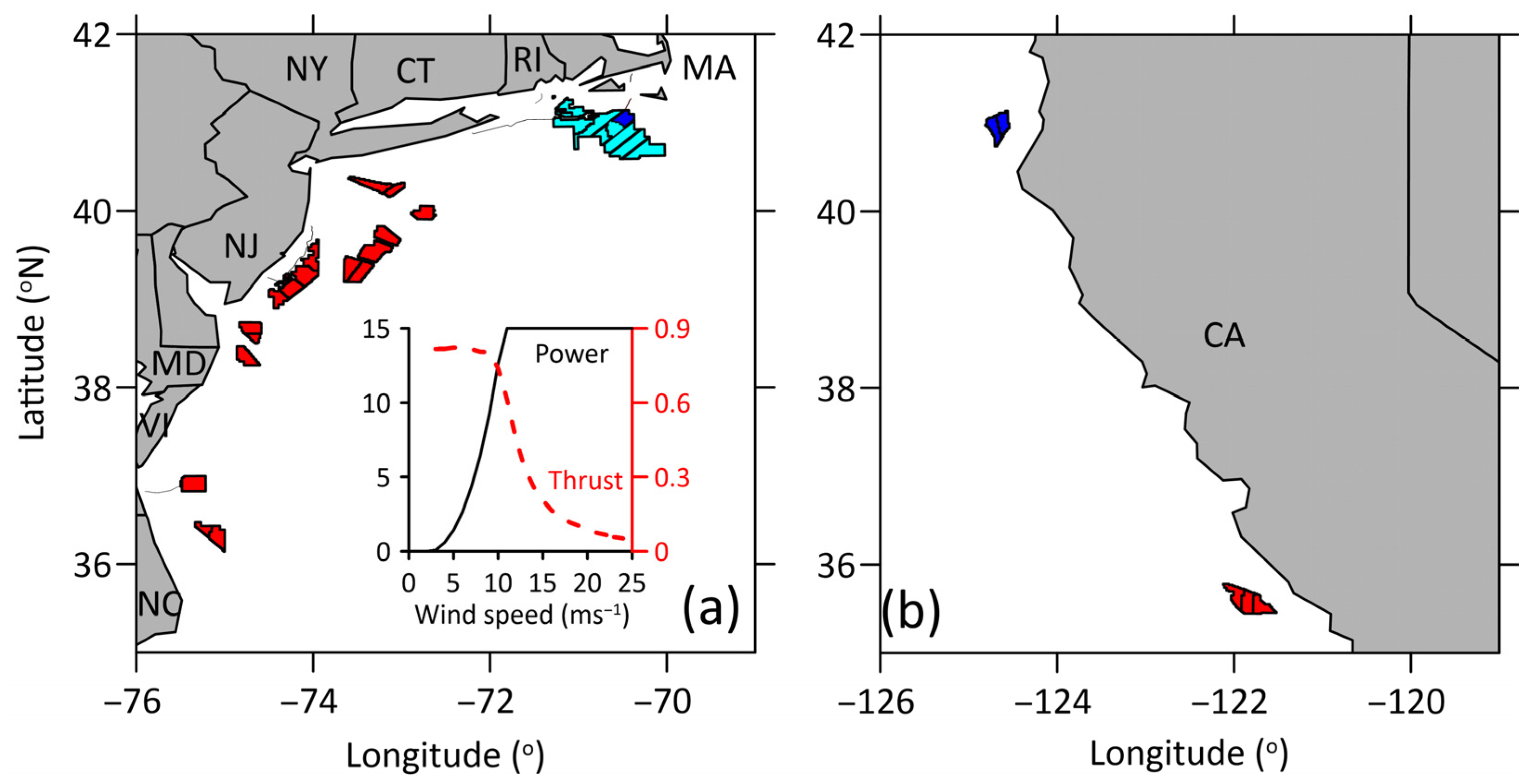
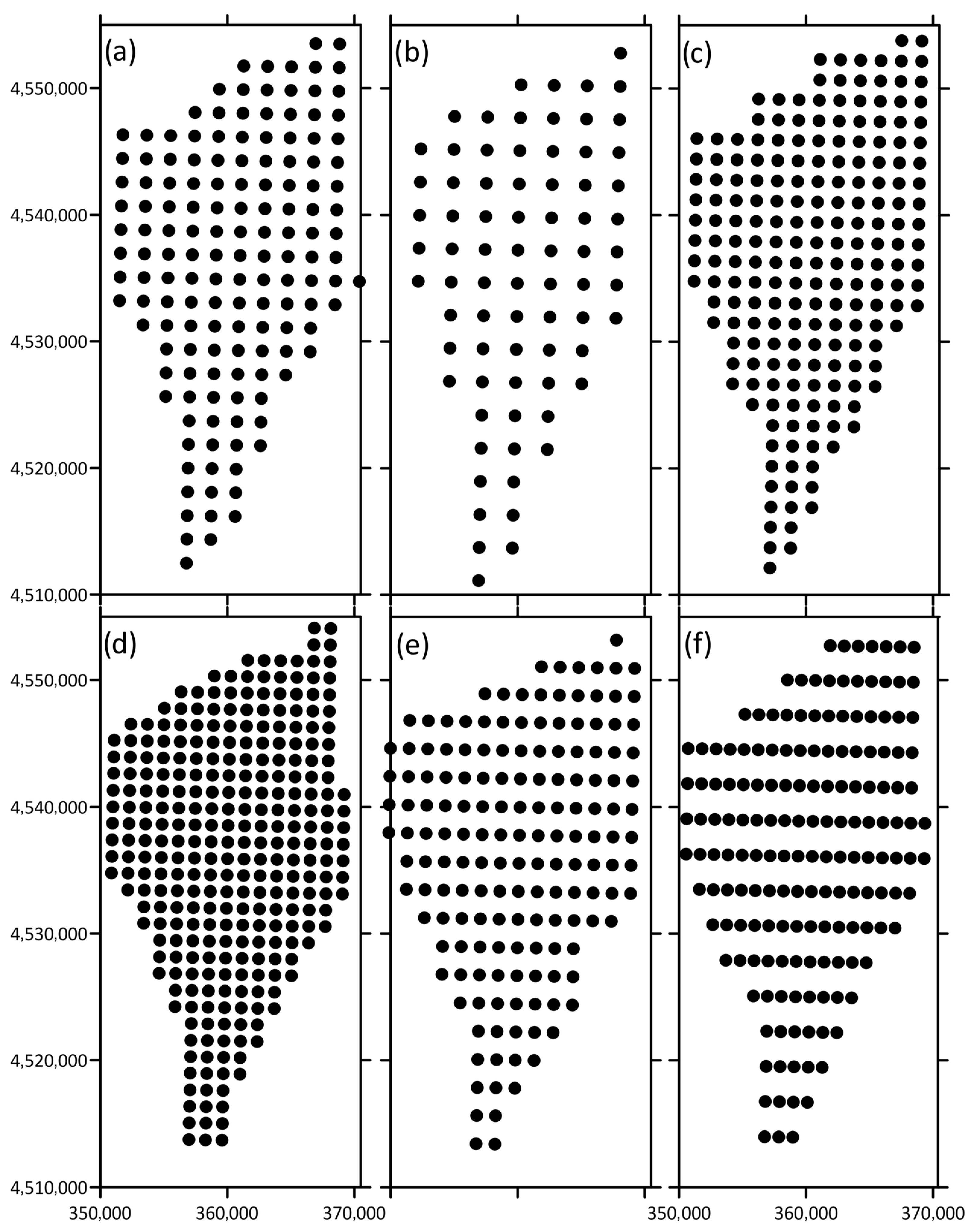
2.2. Wind Farm Design

Before wind farms are constructed, or if exact turbine locations are not available, wake modeling studies require methods to assign plausible locations to provide a given wind turbine spacing or ICD for known LA coordinates [34]. Wind turbine properties (e.g., hub-height, rated capacity, rotor diameter, power and thrust curves) are also needed. For some LA likely wind turbine locations have been published (e.g., coordinates for Vineyard I are available at https://www.boem.gov/renewable-energy/state-activities/vineyard-wind-construction-and-operations-plan-cop-volume-i, accessed on 30 November 2023). Increasing the number of wind turbines (and hence decreasing the spacing below ~4 D) in each area will increase AEP but may not be cost effective because of wake losses and additional turbine loading. Increasing turbine spacing within a given area reduces the number of wind turbines that can be deployed and reduces overall loading but increases cable costs so the likely upper limit is likely ~10 D. Thus, the spacing considered herein and associated ICD is informed by these limits.

The method used here to define wind turbine positions follows previous research [8]. In brief, the first wind turbine location is chosen as the northeast corner of the LA, the next turbine is assigned a location directly south at the specified turbine spacing and so on until the southern edge of the LA is reached. The second column of turbines is assigned starting at the given turbine spacing west of the first turbine if it is within the LA, and so on until the entire LA is filled with turbines. Figure 2 shows the wind turbine locations for the MA and HU LA for the control (CNTR) layout that employs a wind turbine spacing of 1.85 km, because this has been agreed for the MA LA [36]. The IEA 15 MW reference wind turbine [39] is used because the power and thrust curves are readily available and the dimensions are similar to the GE Haliade 13 MW that is being deployed offshore in the US [17]. This gives an ICD of ~4.2–4.4 MW km⁻² for the US east coast LA. Using this method the VY LA comprises 72 wind turbines for the CNTR layout (Figure 2a). Note the number of turbines and ICD varies slightly according to the shape of the LA and how close the turbines are to the edge of the defined area.

Previous research has shown that rotating wind turbine rows and columns away from north–south, east–west so that the spacing is largest in the prevailing wind direction has a relatively minor impact on AEP and wake losses from very large offshore wind energy arrays that are based in diverse multi-directional wind climates such as the US east coast [8]. Thus, while a range of ICD is explored here all layouts are oriented north–south, east–west with equidistant spacing for the US east coast LA. As discussed in detail below, the wind climate for Humboldt indicates strong evidence of channeling and thus a dominance of winds align along a north–south axis. Accordingly, a range of layouts are considered herein including some where the wind turbine spacing in the north–south and west–east axes differ (Figure 3). However, the impact of wind direction on power output may be revisited [40] when wake control scenarios are considered [41].

2.3. Meteorological Data

The generation of a wake by a wind turbine is largely determined by the thrust coefficient and hence is a strong function of inflow wind speed (see inset to Figure 1a). The subsequent recovery of individual wakes and the combination of wakes from different wind turbines is further dictated by the turbulence intensity, planetary boundary layer depth and wind directional variability. Thus, the meteorological dataset used to describe the prevailing atmospheric conditions has the potential to play a key role in wake loss estimation. To quantify this effect, three datasets are used here to derive estimates of the prevailing wind climate for the microscale wake modeling:

(1)

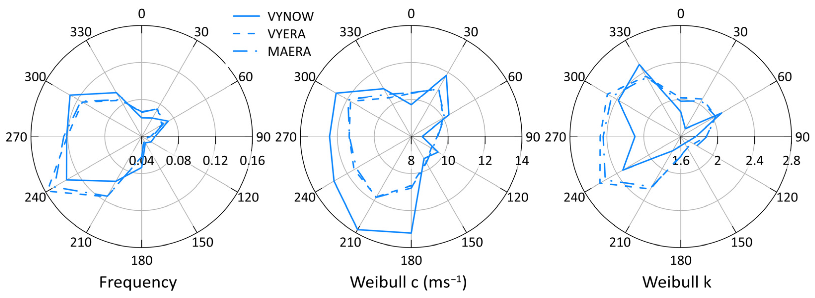
ERA5 reanalysis dataset [42]. Hourly u- and v-wind components at 100 m height from 1979 to 2018 were used to compute wind speeds and directions. The abbreviations used to refer to these data are XXERA, where XX denotes the location:

• NJERA refers to a central location in a group of LA close to New York (NY), New Jersey (NJ) and Maryland (MD) for 1979–2018 [42]. The mean wind speed at 100 m height based on ERA5 data is 8.6 ms⁻¹ and the 50-year return period value is ~34 ms⁻¹ [35].
• MAERA refers to a central location in the group of continuous LA close to Massachusetts/Rhode Island for 1979–2018 [42]. The mean wind speed at 100 m height based on ERA5 data is 9.2 ms⁻¹ for the most central LA and the 50-year return period is ~37 ms⁻¹ [35].
• VYERA for a central location of the Vineyard LA [42] prior to the LA being divided into Vineyard Wind I (VY) and Vineyard Wind. The mean wind speed at 100 m height based on ERA5 data is 9.2 ms⁻¹ and the 50-year return period value is ~36 ms⁻¹ [35].
• HUERA for a central location for the Humboldt LA. The mean wind speed is 9.3 ms⁻¹ at 150 m height from the onsite floating lidar measurements (long-term adjusted using ERA5) [43].

(2)

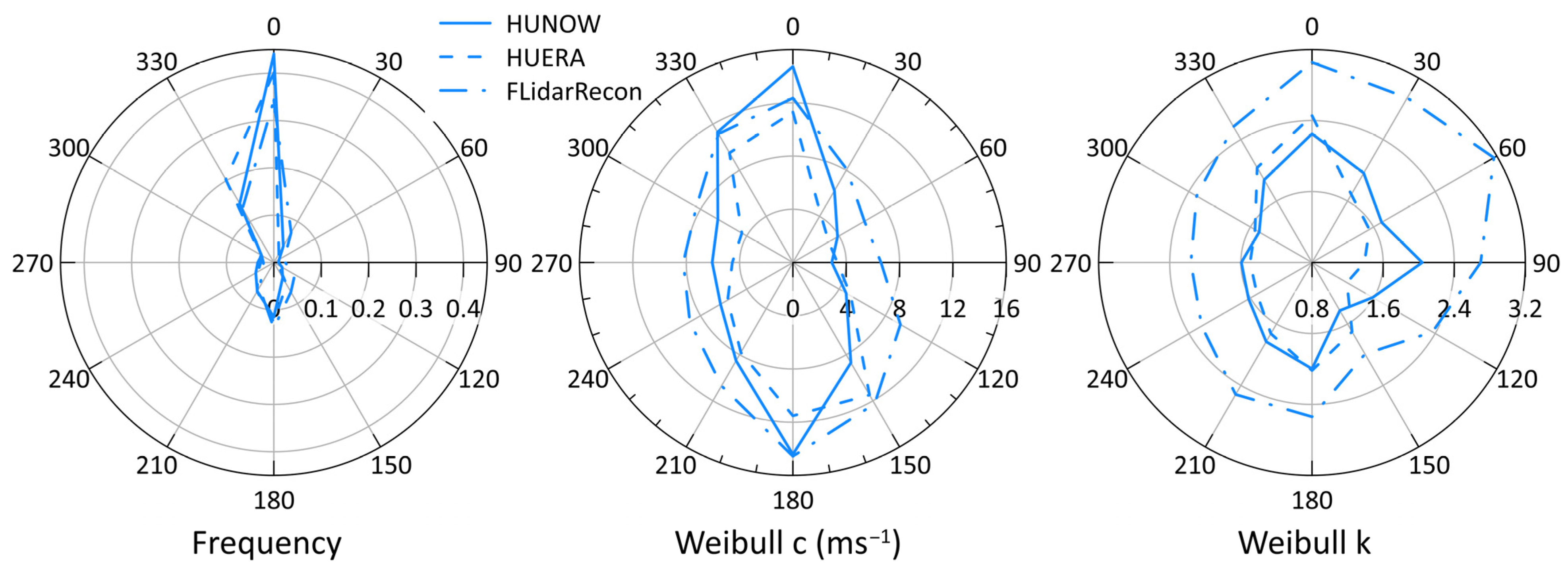
National Renewable Energy Laboratory (NREL) National Offshore Wind dataset (NOW-23) [44] comprises output from a twenty-one-year simulation with the Weather Research and Forecasting (WRF) model. Wind speeds and directions at 150 m were extracted for both Humboldt and Vineyard locations (HUNOW and VYNOW).

(3)

Buoy datasets. For Humboldt LA, in addition to the WRF and ERA5 datasets described above, data from a floating lidar buoy are available (FLidar) [43]. The Leosphere Windcube 866 was deployed off the coast of California at 40.97° N and 124.59° W in a water depth of ~580 m. The data period used here is 8 October 2020 to 29 June 2022 and there are 12 measurement heights from 40 m to 240 m in 20 m intervals, with data collected at additional height of 90 m. It is challenging to maintain a measurement stream from the floating lidar and so the number of observations in each calendar month varies from 2588 in March to 8497 in June. To create a representative dataset Flidar data were ‘corrected’ to a long-term dataset using the measure-correlate-predict method described below [45]. The data are from National Data Buoy Center (NDBC) buoy 46022 height for 1982–2022 [46]. The NDBC buoy location is 40.748° N, 124.527° W and it operates in water depth of 456 m. The dataset is nearly complete with very few years having less than 50% data recovery, and overall data recovery is 82.5%.

The data period for the FLidar at Humboldt is short and thus measure-correlate-predict was used to reconstruct a climatological record of 160 m wind speeds (Recon) based on the NDBC buoy data as follows:

• Identify overlapping 10 min wind speed periods in 2020, 2021 and 2022 (a total of 58,305 10 min periods) between FLidar at 160 m height and the NDBC buoy 3.7 m wind speeds. The seasonal distribution of the overlapping data is December, January, February; 22.7%, March, April, May; 21.2% June, July, August; 28.8%, September, October, November; 27.2% which is broadly representative for this purpose.
• Use linear regression to find a relationship between the 10 min NDBC buoy wind speeds at 3.8 m height to FLidar at 160 m from these overlapping data:

$${\mathrm{U}}_{\mathrm{l}\mathrm{i}\mathrm{d}\mathrm{a}\mathrm{r}}={1.335\mathrm{U}}_{\mathrm{b}\mathrm{u}\mathrm{o}\mathrm{y}}+2.56$$

(4)

• Apply Equation (4) to reconstruct wind speeds at 160 m (Recon) for 1982–2022 at Humboldt LA.
• Wind directions were used directly from the NDBC data buoy 46022 without any adjustment.
• In the following simulations, the reconstructed dataset (Recon) is used in preference to the Flidar data.

Two approaches are frequently used to vertically extrapolate wind speeds to the wind turbine hub-height [47]: (1) The logarithmic wind speed profile for the near-neutrally stratified surface layer:

$${\mathrm{U}}_{\mathrm{z}}={\displaystyle \frac{{\mathrm{u}}_{⁎}}{\mathrm{k}}}\ln \left({\displaystyle \frac{\mathrm{z}}{{\mathrm{z}}_0}}\right)$$

(5)

where U_z is the wind speed at height z, u_* is the friction velocity, κ is the von Karman constant, z₀ is the surface roughness which has a mean value of 0.0002 m for offshore [47]. (2) The power law:

$${\mathrm{U}}_1={\mathrm{U}}_2{\left({\displaystyle \frac{{\mathrm{z}}_1}{{\mathrm{z}}_2}}\right)}^{\mathsf{\alpha }}$$

(6)

where U₁ and U₂ are the wind speeds at height z₁ and z₂, α is the wind shear exponent which is assumed to be 0.14 for offshore [48]. Use of Equation (5) yields a multiplier of 1.031 when extrapolating from 100 m to 150 m. Equation (6), as used within the PyWake system (Version v1.0.10), yields a multiplier on 100 m to 150 m wind speeds of 1.058.

In some analyses presented herein, the wind climate is specified using Weibull parameters in wind directional sectors. The two-parameter Weibull probability distribution is frequently employed within the wind energy industry [49] and has the form:

$$\mathrm{p}\left(\mathrm{U}\right)={\displaystyle \frac{\mathrm{k}}{\mathrm{c}}}{\left({\displaystyle \frac{\mathrm{U}}{\mathrm{A}}}\right)}^{\mathrm{k}-1}\mathrm{e}\mathrm{x}\mathrm{p}\left(-{\left({\displaystyle \frac{\mathrm{U}}{\mathrm{c}}}\right)}^{\mathrm{k}}\right)$$

(7)

where c and k are the Weibull scale and shape parameters that are fitted using maximum likelihood estimation to wind speeds (U).

2.4. Wake Modeling: Microscale

The primary goal of this research is to examine the sensitivity of AEP and wake loss projections for very large offshore wind farms to (i) layout, (ii) meteorological data source and (iii) wake parameterization. Thus, in most of the research presented we employ wake parameterizations within engineering models. These models are useful for optimizing wind turbine spacing and, reproduce with relatively high fidelity, velocity deficits and turbulence intensity changes in wakes as they develop and move downstream [50,51] but without feedback to the atmosphere. Individual wake characteristics such as wake width and velocity deficit are calculated and wakes are combined. Wake superposition is used to combine velocity deficits in overlapping wakes and the relative simplicity of the parameterizations allows the wakes of hundreds to thousands of wind turbines to be calculated [8]. The lack of full coupling (feedback) to the atmosphere means they tend to under-estimate the magnitude of the deep wake in the center of offshore wind farms because the limit on the transfer of momentum downwards into the array is not included [30,52]. Further, the wake recovery downstream of the wind farm is too rapid compared with satellite observations [53].

The PyWake platform [54] is employed herein to generate power production of individual turbines and whole wind farm AEP for a range of steady state conditions because it is open-source, straightforward, computationally efficient and allows comparison of different wake parameterizations. As a minimum, inputs to PyWake are:

• Wind turbine locations (in UTM)
• Wind turbine power and thrust curves, and dimensions
• Site wind climate (Frequency, Weibull scale and shape parameters in twelve directional sectors).

The wake parameterizations used in this work are selected to represent a range of complexities and approaches (

Table 1. Description of the platforms and the wake parameterizations used in the models.

Platform	Wake Parameterization	Description		References
PyWake		Microscale: detailed individual wakes. Limited atmospheric feedback (i.e., wind farm wakes negligible)		[54]
PyWake	NOJ	Standard and first wake parameterization. Linear expansion and analytical multiple wake solution. It defines the wind speed in the wake (Uwake) from a single wind turbine as a function of downstream distance as follows:		[50,55,56,57]
		${\mathrm{U}}_{\mathrm{w}\mathrm{a}\mathrm{k}\mathrm{e}}={\mathrm{U}}_{\mathrm{f}\mathrm{r}\mathrm{e}\mathrm{e}\mathrm{s}\mathrm{t}\mathrm{r}\mathrm{e}\mathrm{a}\mathrm{m}}\left[1-(1-\sqrt{1-{\mathrm{C}}_{\mathrm{t}}}){\left({\displaystyle \frac{{\mathrm{D}}_{\mathrm{w}}}{{\mathrm{D}}_{\mathrm{w}}+2\mathrm{k}\mathrm{X}}}\right)}^2\right]$	(8)
		where Ct is the wind turbine thrust coefficient, Dw is the wake diameter, X is the distance downstream and k is the expansion coefficient which is physically related to roughness length and stability and is typically set to 0.05 for offshore applications. NOJ is also employed in the WAsP Program and is the only one that uses a ‘top-hat’ wake shape rather than a Gaussian profile. Velocity deficit in multiple wakes uses the sum of squares approach. NOJ is frequently used because of its fast and robust performance although it underestimates wake propagation downstream of large offshore arrays.
PyWake	Fuga	Fuga is based on a linearized Reynolds Averaging Navier–Stokes approach that tracks individual, embedded wakes. It was explicitly developed for offshore wind farms It uses a set of Look Up Tables (LUT) for particular roughness length and stability criteria. Use of LUT to store intermediate results speeds up the calculations many-fold and allows the wakes of many wind turbines and the far downstream wake to be determined. To calculate the combined velocity deficit for multiple wakes the linear superposition approach is used.		[58,59]
PyWake	FugaB	As Fuga but includes upstream blockage. Similar wake losses to Fuga with additional blockage effect of ~1–2% AEP loss. Requires more computing resources than Fuga. Fuga Blockage includes the decrease in wind speed directly upstream of a wind farm in addition to the downstream wake effect. To calculate the combined velocity deficit for multiple wakes the linear superposition approach is used.		[60]
PyWake	TurboGauss (TurboG)	The model is implemented based on TurboPark using the Gaussian wake shape with a non-linear turbulence-dependent wake expansion coefficient [61] that decreases with downstream distance from the turbine. TurboPark gives unbiased estimates of wake losses in comparison with SCADA data from European offshore wind farms. To calculate the combined velocity deficit for multiple wakes the sum of squares approach is used.		[61,62,63]
PyWake	BastankhahGaussianDeficit (BG)	There are several versions of this analytical model which applies mass and momentum conservation in the wake and uses Gaussian wake shape with linear wake expansion. It uses Ct and requires a wake expansion coefficient (k) to be defined. Here k is set to 0.032455. To calculate the combined velocity deficit for multiple wakes the sum of squares approach is used. It generally scales with ICD in a similar manner to NOJ, but with larger wake losses.		[64]
PyWake	GLC	An analytic approach that uses the thin shear layer approximation of the Navier–Stokes equations as the basis of an axisymmetric wake expansion that employs a Gaussian shape wake e coefficient that depends on the thrust coefficient and turbulence intensity. To calculate the combined velocity deficit for multiple wakes the linear superposition approach is used.		[65]
WRF		Mesoscale model requires high-performance computing (HPC). Atmospheric feedback to wind speed, planetary boundary layer structure and turbulence intensity. Limited individual wake details via a wind farm parameterization (WFP) but full wind farm wakes modeled.		[66,67]
	Fitch	Default WFP in WRF. No in grid wake expansion. Momentum extracted from the rotor plane. Turbulent Kinetic Energy (TKE) added as function of wind turbine thrust coefficient.		[68,69,70]
	EWP	Gaussian form for momentum extraction which thus extends vertically beyond the rotor plane. Within grid wake expansion treated. TKE only added via shear.		[71,72]

). The simulations were run with default values for parameters such as the Look Up Tables in Fuga and the wake expansion coefficient in NOJ. To calculate the combined velocity deficit for multiple superimposed wakes, two approaches are employed. The default is the linear superposition approach wherein the velocity deficit in the merged wake is the linear sum of the velocity deficit in wakes that are being superimposed. Some wake parameterizations employ the sum of squares approach; wherein the velocity deficit within a combined wake is the square-root of the sum of the squared velocity deficits from the merged wakes.

Two scales of PyWake simulations are presented (1) the entire US east coastal area that contains multiple LA clusters and comprises 2617 wind turbines and (2) for individual clusters/LA. These simulations are performed on a Jetstream large memory instance with 500 GB of RAM and 64 CPU (https://docs.jetstream-cloud.org/overview/config/#large-memory-nodes-32-nodes, accessed on 9 July 2025), typically taking from seconds (NOJ) to minutes (Fuga) to complete the climatologically representative simulations.

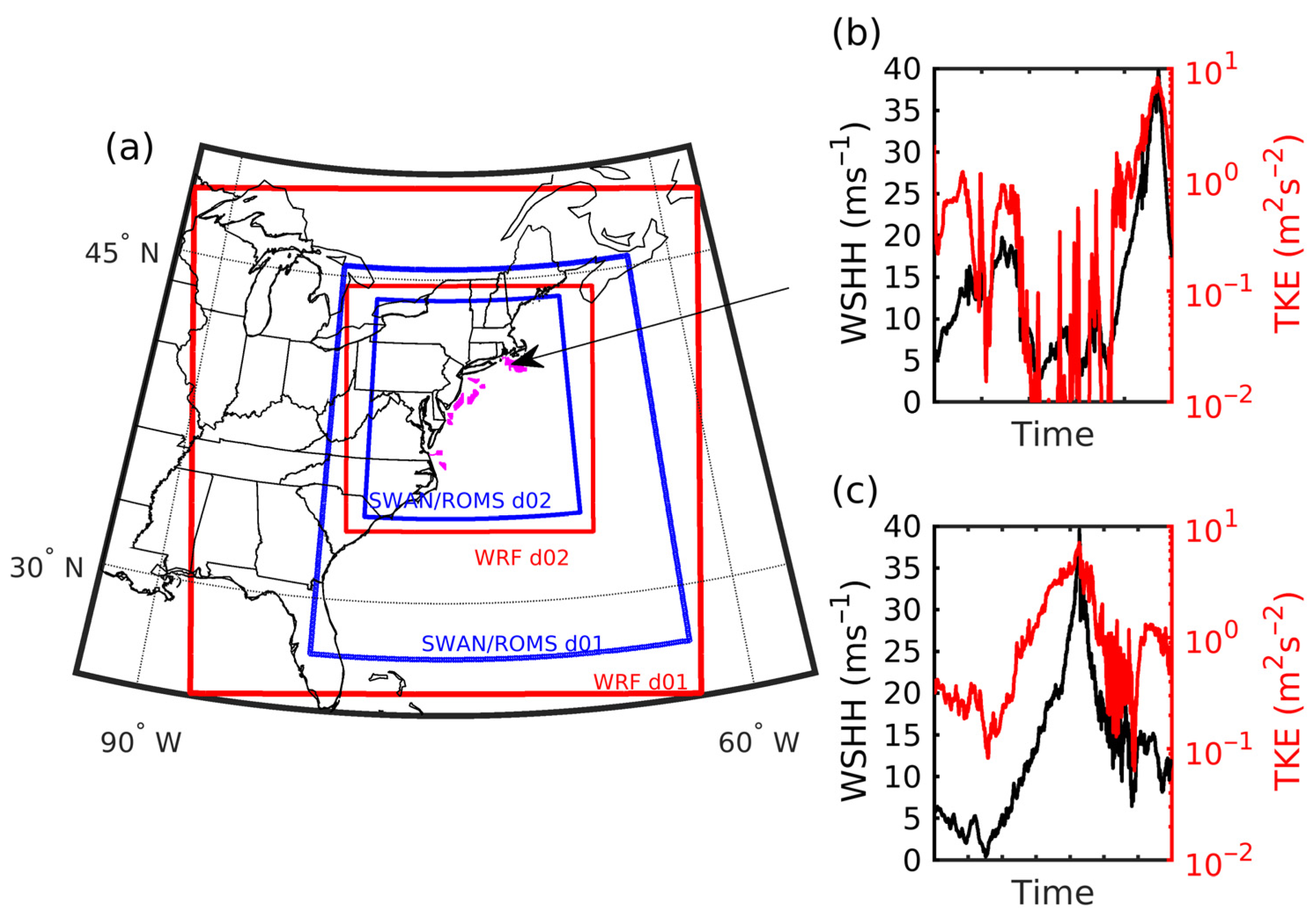
2.5. Wake Modeling: Mesoscale

Engineering wake models can efficiently run simulations for thousands of wind turbines arranged in different layouts and ICD, but this comes at a cost in terms of the specification of the spatial variability in atmospheric conditions and full two-way coupling between the wakes and the atmosphere. Atmospheric mesoscale models such as the Weather Research and Forecasting (WRF) model are designed to model atmospheric physics in detail and can be used to quantify whole wind farm wakes over tens of kilometers [7,17] using wind farm parameterizations (WFP) that treat wake dynamics in a simplified manner. Most WRF simulations have employed one of two WFP; Fitch [69] as modified in [70] and the Explicit Wake Parameterization [71]. The most consequential differences between these are the addition of turbulent kinetic energy (TKE) in Fitch that is parameterized as a function of the wind turbine thrust coefficient and the dissipation of the wake and assignment of length scale in EWP which means results can be resolution dependent [72]. For offshore conditions when these parameterizations are employed in high-resolution simulations, Fitch gives higher wake losses/lower CF than EWP resulting in a difference of nearly 20% in AEP for the US offshore LA [7]. Herein we present results from prior WRF simulations that used ERA5 for the initial and lateral boundary conditions (LBC) and employed both EWP and Fitch WFP to contextualize the PyWake analyses.

As described above, a major source of uncertainty in wake modeling is the structure of the lower atmosphere and specifically the thermal stratification, ambient turbulence intensity (TKE), planetary boundary layer height (PBLH), and veer and shear in the wind speed profile that dictate hub-height wind speeds. Indeed, a simple statistical emulator of based solely on hub-height wind speed, PBLH and TKE was found to reproduce 85% of the variance in WRF-derived estimates of whole wind farm wake spatial extent [30]. Since these lower-atmosphere properties are strongly dependent on atmosphere-surface coupling and both thermal and mechanical generation of eddies, it has been postulated that mesoscale simulations wind farm wake extents and implications for power production may fundamentally differ in simulations with an atmosphere-only version of WRF versus one in which the atmosphere is dynamically coupled to a surface wave and ocean model.

Results from a preliminary study of a two-week period focused on the German Bight region in the North Sea found the mean whole wind farm wake length (downwind distance at which the wind speed had recovered to 95% of the freestream value) from WRF and Coupled Ocean-Atmosphere-Wave-Sediment Transport (COAWST) simulations differed by up to 25% [73]. Further, power production from individual wind turbines and wind farms differed by up to 15%. Thus, we present new mesoscale simulations to explore the role of atmosphere-ocean coupling in wake magnitudes. They are performed with WRF (v4.2.2) and with the COAWST modeling system (v3.7) [74] (configured with WRF v4.2.2, Regional Ocean Modeling System (ROMS) v3.9 and Simulating Waves Nearshore (SWAN) v41.31) with the model components interacting through use of the Model Coupling Toolkit (MCT) (v2.6.0) every 10 min. The WRF/COAWST simulations were run on the Perlmutter supercomputer owned and operated by the United States Department of Energy. Each simulation was performed using 2 nodes, with 128 processors per node. The 256 processors requested for the COAWST simulations were divided, with 225 for WRF, 20 for ROMS, and 11 for SWAN. This split is to ensure each model component takes a similar amount of time to reach the coupling interval and therefore allows the overall simulation to run more efficiently. To keep continuity, WRF simulations also employed 225 processors. This continuity also means that COAWST and WRF simulations each took ~36 h for each 1 calendar day of simulation. The availability of HPC resources is thus an important factor in the type and scale of mesoscale simulations that can be performed.

Each period is simulated without wind turbines (noWT) and then again with wind turbines (WT) deployed in all LA. Both WRF and COAWST simulations with the action of wind turbines included use the Fitch WFP and the 15 MW reference wind turbine for the CNTR layout. Both WRF and SWAN/ROMS use nested domains (Figure 4a). The two WRF domains have grid spacing (dx) of 4 km and 1.33 km, respectively, and use 72 vertical levels.

Grid spacing for ROMS and SWAN in the two domains are 10 km and 3.33 km, respectively. Full details of the simulations and comprehensive evaluation of the noWT simulations relative to observations are given in ref. [67]. The two simulation periods are 1200 UTC on 24 August 2011 through 1200 UTC on 29 August 2011 and 1200 UTC on 25 October 2012 through 1200 UTC on 1 November 2012. They represent very dynamic flow conditions and thus high variability in the freestream wind speeds and turbulent kinetic energy (TKE, from the MYNN2 planetary boundary layer scheme) at hub-height (Figure 4b,c). Both include interludes when the freestream hub-height wind speed in the center of the MA LA cluster exceeds the cut-out wind speed of the IEA 15 MW reference turbine due to the passage of tropical cyclones [67]. Of particular importance to this research both the WRF and COAWST simulations implement a maximum ocean roughness drag coefficient of 2.85 × 10⁻³ to account for the asymptotic behavior of surface roughness length (z₀) at high wind speeds.

Wind speed differences due to the action of wind turbines are computed as the mean WS without wind turbines (noWT) minus the WS from the simulation with wind turbine (WT). Thus, wind speed differences (velocity deficits) due to wakes will be positive. Normalized wake-induced power production losses are derived from the paired simulations (noWT vs. WT) and computed as follows:

$${\mathrm{w}\mathrm{a}\mathrm{k}\mathrm{e}\mathrm{l}\mathrm{o}\mathrm{s}\mathrm{s}}_{\mathrm{x},\mathrm{y}}={\displaystyle \frac{{\sum }_1^{\mathrm{i}=\mathrm{n}}\left(\mathrm{P}\mathrm{C}\left({\mathrm{W}\mathrm{S}(\mathrm{x},\mathrm{y},\mathrm{i})}_{\mathrm{n}\mathrm{o}\mathrm{W}\mathrm{T}}\right)\right)-{\sum }_1^{\mathrm{i}=\mathrm{n}}\left(\mathrm{F}\mathrm{i}\mathrm{t}\mathrm{c}\mathrm{h}\left({\mathrm{W}\mathrm{S}(\mathrm{x},\mathrm{y},\mathrm{i})}_{\mathrm{W}\mathrm{T}}\right)\right)}{{\sum }_1^{\mathrm{i}=\mathrm{n}}\left(\mathrm{P}\mathrm{C}\left({\mathrm{W}\mathrm{S}(\mathrm{x},\mathrm{y},\mathrm{i})}_{\mathrm{n}\mathrm{o}\mathrm{W}\mathrm{T}}\right)\right)}}\times 100$$

(9)

where i denotes the output time stamps from 1 to n, where n is the number of 10 min output periods of the simulation. PC is the power production as a function of wind speed (WS) in that grid cell (x,y) and time (i) computed by applying the power curve for the IEA 15 MW reference wind turbine to wind speeds at hub-height from the noWT simulation. Fitch is the power production from those same grid cell and time stamp for the paired WT simulation. Thus, wake-induced power losses are positive.

3. Results from Microscale Wake Modeling

3.1. All East Coast LA

The spatial patterns and total magnitude of wake losses for the offshore LA vary considerably depending on the wake parameterization used. Figure 5 illustrates wake loss spatial distribution as simulated by the PyWake program with the NOJ and Fuga wake parameterization across the 2617 turbines in the east coast of LA and the wind climate derived from ERA5 (ERANJ). Using NOJ (Figure 5a) indicates total power production of 181 TWh/yr, which would be approximately 4.5% of the total electricity use of the USA in 2022 [75]. The average CF is 53.1% and the overall wake loss of 4.4% represents a significant reduction in potential energy production, impacting project economics and feasibility (Figure 5a). Consistent with the discussion above, regarding the rapid dissipation of wakes in this parameterization, there is no obvious interaction from wakes between the different LA. Simulations of the same layout and wind climate using the Fuga wake parameterization yield total power predictions of 170 TWh/yr (6% lower than NOJ) and the average CF is 49.4%. The overall wake loss is 11.1% and the wakes in the center of the LA are considerably deeper reaching 19% in the center of the MA LA (Figure 5b). The three most southerly NE LA act as one continuous area and the wakes are deeper and are propagated further using Fuga. Apart from these three LA, wind wake wind shadows are less spatially extensive than are indicated by WRF [30]. For comparison, WRF simulations for the same turbine locations (but excluding the LA off the coast of Virginia, VA) indicate an average CF of 53.2% for simulations using EWP and 42.6% from Fitch.

Further PyWake simulations in the remainder of the paper are performed on smaller domains to allow detailed quantification of differences in annual electricity production (AEP), capacity factors (CF) and wake losses from different wind turbine layouts (spacing, ICD) and wind climates.

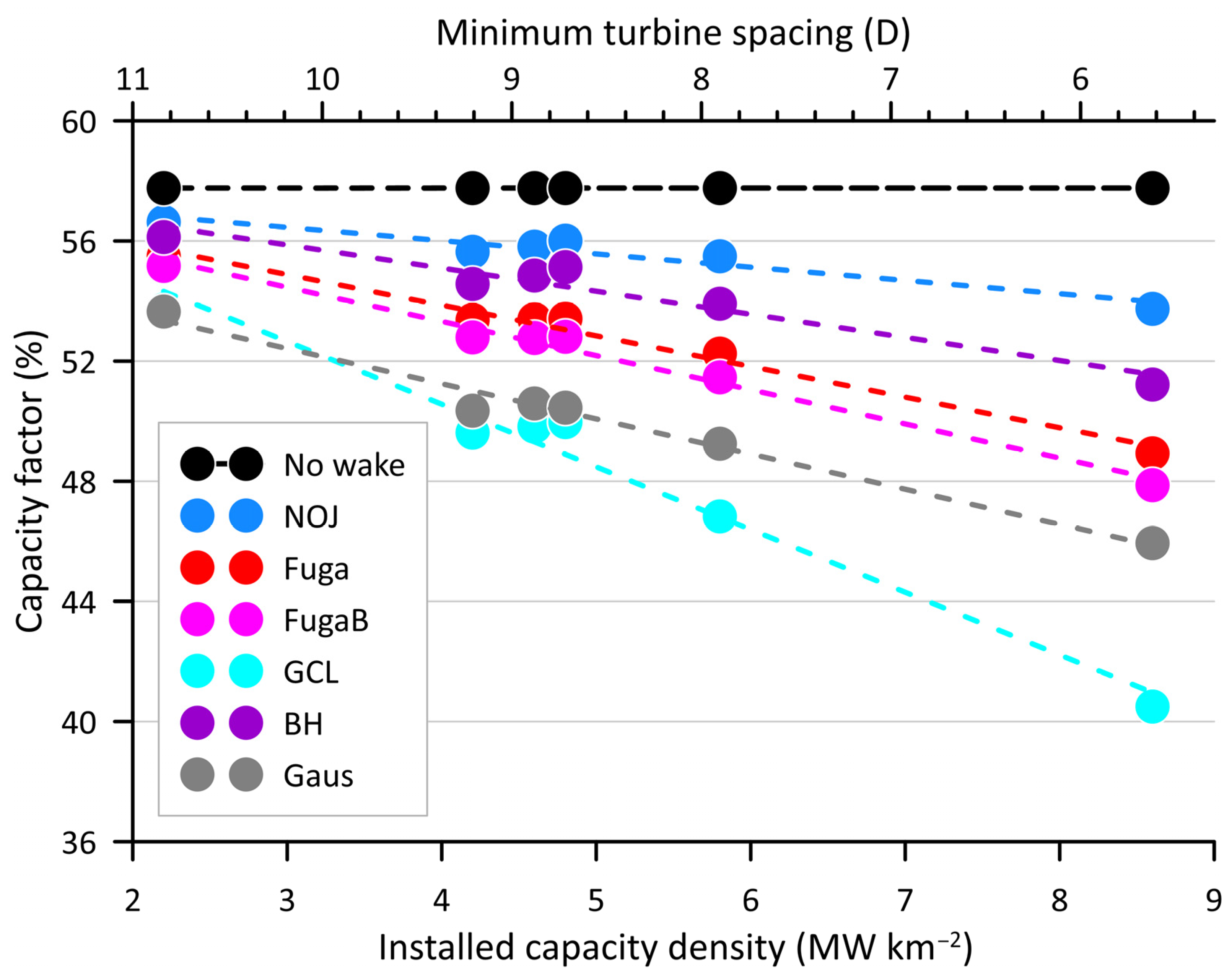
3.2. Sensitivity of AEP and CF to Installed Capacity Density

3.2.1. MA

The impact on AEP and CF from different wind turbine ICD over the MA LA based on PyWake simulations with the MAERA wind climate are shown in Figure 6 along with climatologically derived estimates based on simulations with both the Fitch and EWP wind farm parameterizations in WRF. CF decline markedly and broadly linearly with ICD increasing from 2 to 9 MW km⁻². Consistent with Figure 5, CF are higher in simulations with NOJ than other wake parameterizations for all ICD considered. It is important to note that the sensitivity of CF to ICD is wake model dependent. Mean CF for the range of ICD considered span nearly 4 percentage points from NOJ and over 10 percentage points with Fuga (slightly more with FugaB), which is a substantial difference in terms of expected AEP (and hence LCoE). BG is a modified version of NOJ (using a Gaussian wake profile) and gives similar results with slightly larger wake losses. The wake model that shows the most pronounced change in CF with ICD is GCL. According to the fit regression fit a one unit change in ICD results in a 3.6 percentage point change in CF (

Table 2. Linear regression of Capacity Factor (CF) from different platforms and wake parameterizations for the MA LA as a function of ICD (see Figure 6). The linear regression equation is fitted as $\mathrm{C}\mathrm{F}=\mathrm{m}\times \mathrm{I}\mathrm{C}\mathrm{D}+\mathrm{c}$ where m is the slope, c is the intercept (set to $\mathrm{C}\mathrm{F} \left(\mathrm{N}\mathrm{o}\mathrm{W}\mathrm{T}\right)$) and r² is the coefficient of determination.

Platform and Wake Parameterization	Mean CF (%) for ICD~4.3 MW km−2	Regression Slope (m)	r2
WRF Fitch [30]	42.9	−3.74	0.798
WRF EWP [30]	53.2	−1.59	0.909
PyWake
NoWT	59.8	-	-
NOJ	57.3	−0.55	0.971
Fuga	52.2	−1.68	0.990
FugaB	51.1	−1.91	0.998
GCL	43.3	−3.63	0.986
BG	55.9	−0.88	0.988
Gaus	48.0	−2.41	0.660

). The only wake model that does not exhibit a pseudo-linear response in CF as a function of ICD is the Gaus model (Table 2). In Gaus the intensity of the wake-generated turbulence decreases moving downstream from the turbine and the wake expansion slows down [61].

Although the absolute values of CF differ by simulation platform (microscale v mesoscale) and wake parameterization, there is good agreement in the results between PyWake-Fuga and WRF-EWP and WRF-Fitch and PyWake-GCL (Figure 6). Results from the wake parameterizations are consistent with wake losses being ranked smallest to largest: NOJ; BG; Fuga; FugaB; Gaus and GCL. Differences arising from different wake parameterizations are discussed further in Section 3.4.

3.2.2. Humboldt

There is a potential for AEP at Humboldt to be impacted by the exact configuration of wind turbine layout due to the nearly unidirectional wind rise. Thus, a range of layouts were simulated including those with asymmetry in spacing in the west–east and south–north directions (Figure 3). As for the other LA, AEP for all layouts and ICD considered are persistently lower than Fuga and than NOJ (

Table 3. AEP from PyWake with NOJ or Fuga parameterizations for HU for different ICD and wind turbine layouts (see Figure 3) based on simulations with the Recon wind climate. Spacing is shown for W-E direction × S-N direction in km (and rotor diameters, D). Recall the rotor diameter of the 15 MW IEA reference turbine is 240 m.

Layout	# Turbines	ICD (MW km−2)	Spacing (km)	AEP NOJ (GWh/yr)	AEP Fuga (GWh/yr)
CNTR	151	4.2	1.85 × 1.85 (7.8 × 7.8 D)	11,798	11,215
DOUB	78	2.2	2.6 × 2.2 (10.8 × 9.2 D)	6227	6078
6MWD	208	5.8	1.6 × 1.2 (6.7 × 5.0 D)	16,009	14,856
HALF	306	8.6	1.2 × 1.3 (5.0 × 5.4 D)	22,899	20,358
LONG	164	4.6	1.1 × 2.2 (4.6 × 9.2 D)	12,845	12,164
LLNG	172	4.8	1.0 × 2.8 (4.2 × 11.7 D)	13,517	12,757

). For the CNTR layout the CF from NOJ is 60%, while that from Fuga is 57%. This declines to 58% and 51% for the layout with twice as many wind turbines (HALF). CF can be maintained at the CNTR levels even for ICD of 4.6 or 4.8 MW km⁻² if the north–south (N-S) spacing increases, even when west–east (W-E) spacing decreases to maintain a relatively high ICD. In the LONG scenario increasing N-S spacing by 1.4 D and reducing W-E spacing by 3.2 D gives a slightly higher ICD and 8.9% increase in AEP (NOJ) or 8.5% (Fuga). In the LLNG scenario increasing N-S spacing by 3.9 D and reducing W-E spacing by 3.6 D gives a slightly higher ICD and 14.6% increase in AEP (NOJ) or 13.7% in Fuga compared to CNTR.

3.3. Sensitivity of AEP and CF to Wind Climate

3.3.1. Vineyard Wind I

Vineyard Wind I is in relatively advanced state of construction and thus may operate for some time prior to deployment of wind turbines in adjacent LA. In this section only internal wakes to this wind farm are considered, and we explore the impact of using NOW-23 or ERA5 wind climates. The differences in wind climates for VY are very small, although there are some differences in the distribution of wind speed by wind direction (Figure 7). Use of the VYNOW wind climate yields an AEP that is 0.6% higher and MAERA (which is for the center of the MA LA) is 0.1% lower than is computed using the VYERA wind climate. For comparison, the range of differences in AEP generated by different wake parameterizations but for the same wind climate are around 8 percentage points for MAERA and VYERA and 7 percentage points for VYNOW (

Table 4. Impact of different wind climates and wake parameterizations on power output, CF and wake losses for the 72 wind turbines at VY deployed with ICD of ~4.3 MW km² (CNTR layout).

Wind Climate	VYERA			VYNOW			MAERA
Wake Parameterization	AEP (GWh/yr)	CF (%)	Wake Loss (%)	AEP (GWh/yr)	CF (%)	Wake Loss (%)	AEP (GWh/yr)	CF (%)	Wake Loss (%)
NoWT	5663	59.9	0	5695	60.2	0	5655	59.8	0
NOJ	5466	57.8	3.5	5524	58.4	3.0	5459	57.7	3.5
Fuga	5341	56.5	5.7	5418	57.3	4.9	5335	56.4	5.7
FugaB	5276	55.8	6.8	5360	56.7	5.9	5271	55.7	6.8
GCL	5112	54.0	9.7	5215	55.1	8.4	5107	54.0	9.7
BG	5375	56.8	5.1	5445	57.6	4.3	5368	56.7	5.1
Gaus	5049	53.4	10.8	5161	54.6	9.4	5046	53.3	10.8

).

It is worth noting that assumptions made in the different wake parameterizations and default values used within PyWake regarding the atmospheric profile are also important to the results. Unless otherwise stated, for the simulations here, it is assumed that the turbulence intensity (TI) is 6% at 100 m height based on values in near-neutral conditions at the Nysted offshore wind farm [76]. It is further assumed that the wind shear exponent α is 0.14 [48] (Equation (6)). Changing α naturally changes the wind resource derived from the ERA5 dataset because of the extrapolation of wind speeds to the 150 m turbine hub-height (Equation (6)). To evaluate the impact on the AEP from the Vineyard array, four additional simulations were run for VY with slight variations in TI and α. Increasing α to 0.2, consistent with the relatively high frequency of stable stratification offshore [77], increases AEP by an average of 2.1% across the wake parameterizations due to the increase in wind speeds associated with extrapolation from 100 m to 150 m. Decreasing α to 0.1 (to imply more unstable conditions) decreases AEP by an average of 1.4%. Using α = 0.07 which is the equivalent to a logarithmic profile with roughness length set to 0.0002 m for offshore decreases AEP by an average of 2.4%. Only the GCL and Gaus wake parameterizations use TI directly, while the prevailing stability and TI are encoded within inputs to Fuga and FugaB. For each 1 percentage point decrease in TI, AEP decreases by ~0.8% in GCL, and 0.15% in Gaus. Thus, changing the default settings for TI and α have a smaller impact on AEP, CF and wake losses than changing the wake parameterization and is similar to the effect of selecting one of two highly robust meteorological datasets.

3.3.2. Humboldt

The Recon wind climate for Humboldt exhibits good agreement with HUERA and HUNOW in terms of the sectorial Weibull parameters used in the wake modeling and all sets show the dominance of northerly wind directions (

Table 5. Wind speed datasets used to reconstruct a long-term wind speed dataset at the Humboldt LA along with the mean values and Weibull parameters.

Dataset	Data Period	Number of Observations (%)	Height	Mean Wind Speed (ms−1)	Standard Deviation (ms−1)	Weibull Shape Factor (ms−1)	Weibull Scale Factor
FLidar	2020–22 (overlap)	53,281 (91%) *	160	10.40	5.70	11.73	1.92
NDBC	2020–22 (overlap)	53,281	3.8	5.71	3.27	6.43	1.83
NDBC	1982–2022	305,575 (82.5%)	3.8	5.64	3.45	6.33	1.71
Recon	1982–2022	305,575 (82.5%)	160	10.09	4.61	11.42	2.34

* Reported in [43] accounting for power supply issues.

, Figure 8). Using Recon, the mean wind speed at 160 m height is estimated as 10.09 ms⁻¹ (10.04 ms⁻¹ at 150 m using Equation (5) and an offshore roughness of 0.0002 m) which is higher than mean wind speeds determined from ERA5 (8.66 ms⁻¹ at 150 m). For comparison wind speeds at 100 m height at Humboldt are reported to be 9.75–11.0 ms⁻¹ (10.1–11.4 ms⁻¹ at 160 m) [19] based on 19 years of WRF simulations [78]. Later analyses suggested the wind resource was over-estimated and the average bias could be as high as 1.3 ms⁻¹ at 150 m height at Humboldt [79].

Projected AEP from HU varies substantially when the wind climate at 150 m is derived from HUNOW, ERA5 (extrapolated from 100 m to 150 m using the power law) or Recon (extrapolated down from 160 m using the power law). AEP from Recon averages 6 percentage points higher than NOW-23 and over 16 percentage points from HUERA. In the absence of wake effects, the Recon dataset yields CF that are almost 10 percentage points higher than those from ERA5 (

Table 6. Modeled Annual Energy Production (AEP), Capacity Factors (CF) and wake losses for the Humboldt LA simulated using different wind climates/wake parameterizations for the CNTR layout (ICD~4.3 MW km⁻²).

Wind Climate	HUNOW			HUERA			Recon
Wake Parameterization	AEP (GWh/y)	CF (%)	Wake Loss (%)	AEP (GWh/y)	CF (%)	Wake Loss (%)	AEP (GWh/y)	CF (%)	Wake Loss (%)
NoWT	11,459	61.1	0.0	10,444	52.0	0.0	12,337	61.4	0.0
NOJ	11,040	55.6	3.7	9932	50.1	4.9	11,798	59.5	4.4
Fuga	10,590	53.4	7.6	9409	47.4	9.9	11,215	56.5	9.1
FugaB	10,474	52.8	8.6	9269	46.7	11.3	11,506	58.0	6.7
GCL	9845	49.6	14.1	8601	43.3	17.7	10,305	51.9	16.5
BG	10,828	54.6	5.5	9679	48.8	7.3	11,521	58.1	6.6
Gaus	10,056	50.3	12.2	8780	44.0	15.9	10,485	52.5	15.0

). These differences are of equivalent magnitude to the range of CF from different wake parameterizations indicating the high value of high-fidelity meteorological data. CF in simulations excluding wakes are 52% using HUERA to 61.1% using HUNOW and 61.4% with Recon. These compare to CF of ~50.2% from the FLORIS model simulated using the wind climate from WRF simulations. In the following HUNOW has been selected although there are indications that this may over-predict the wind resource [79], it produces a slightly lower wind resource than Recon (that was independently generated from FLidar and the NDBC buoy dataset) (Table 5).

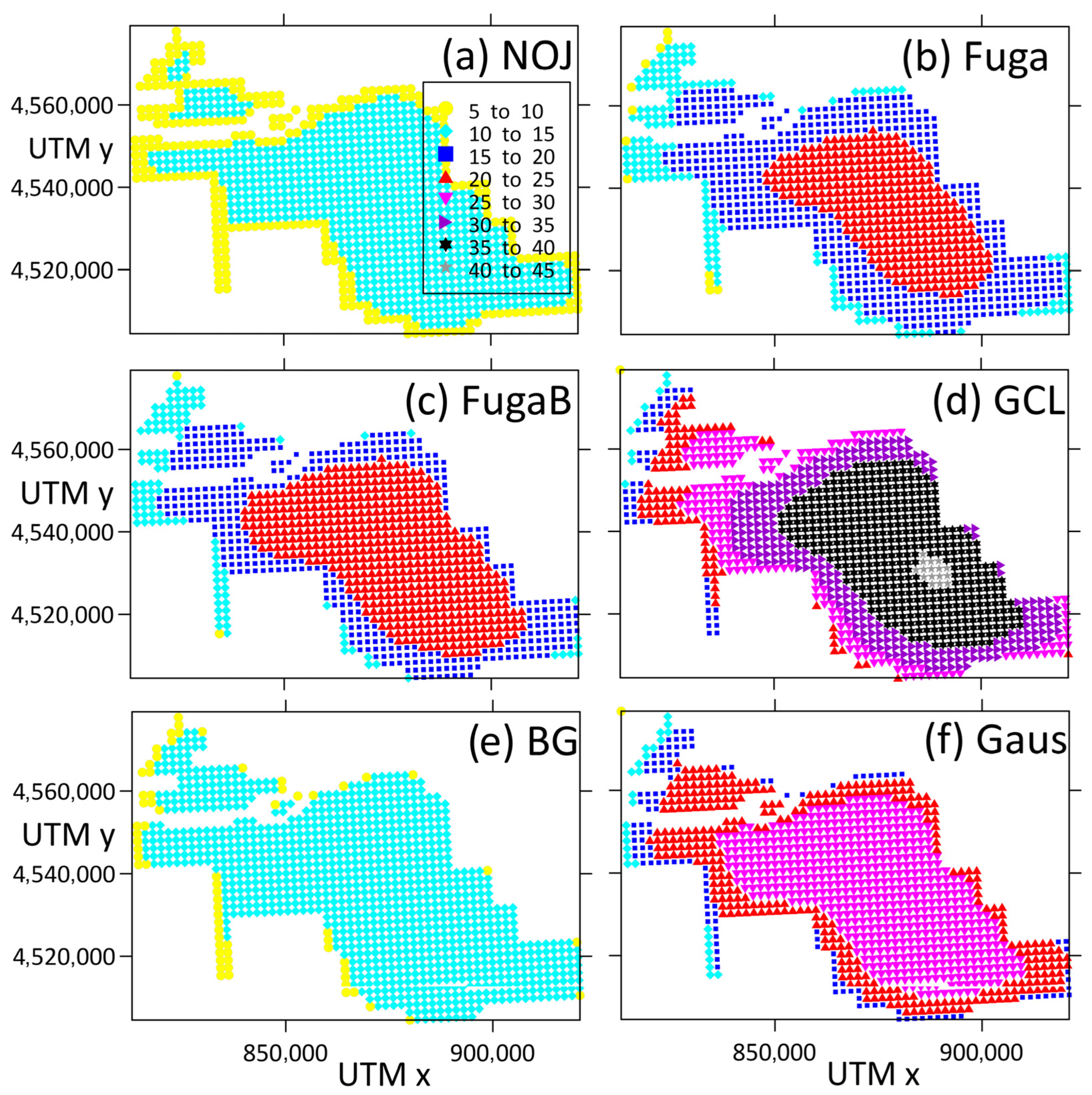
3.4. Sensitivity to Wake Parameterization

3.4.1. MA

Simulations with six wake parameterizations were run for CNTR layout (1066 turbines within MA LA) and the MAERA wind climate. The simulations show different spatial patterns of wake losses as well as absolute values (Figure 9). NOJ predicts wake losses of 7–11% for all turbines, BG predicts 7–13% wake losses (average 12.3%) but neither evolves a deep array effect and both are likely underestimating wake losses based on previous evaluations [63,76]. Fuga simulates greater loss of AEP within the center of the full array (a deep array effect), with wake losses of up to 22% at some wind turbines. FugaB has slightly higher wake losses than Fuga and similar spatial patterns. GCL exhibits the largest deep array effect with wake losses over 40% at some central wind turbines and Gaus predicts wake losses of up to 30% at some locations. The array averaged wake losses from these parameterizations are 10.1% (NOJ), 18.1% (Fuga), 19.3% (FugaB), 32.1% (GCL), 12.3% (BG) and 24.6% (Gaus). For comparison, mean climatologically representative wake losses for all east coast LA as computed using WRF with the Fitch and EWP parameterizations range from 27 to 37% and 11 to 19%, respectively [30].

3.4.2. Humboldt

Simulations with six different wake parameterizations were performed for the layouts shown in Figure 3 for the Humboldt LA using the HUNOW wind climate. Recall these layouts span an ICD range of 2.2 MW km⁻² to 8.8 MW km⁻² and thus likely covers the plausible range of values that could be realized. The results (Figure 10) show three key features:

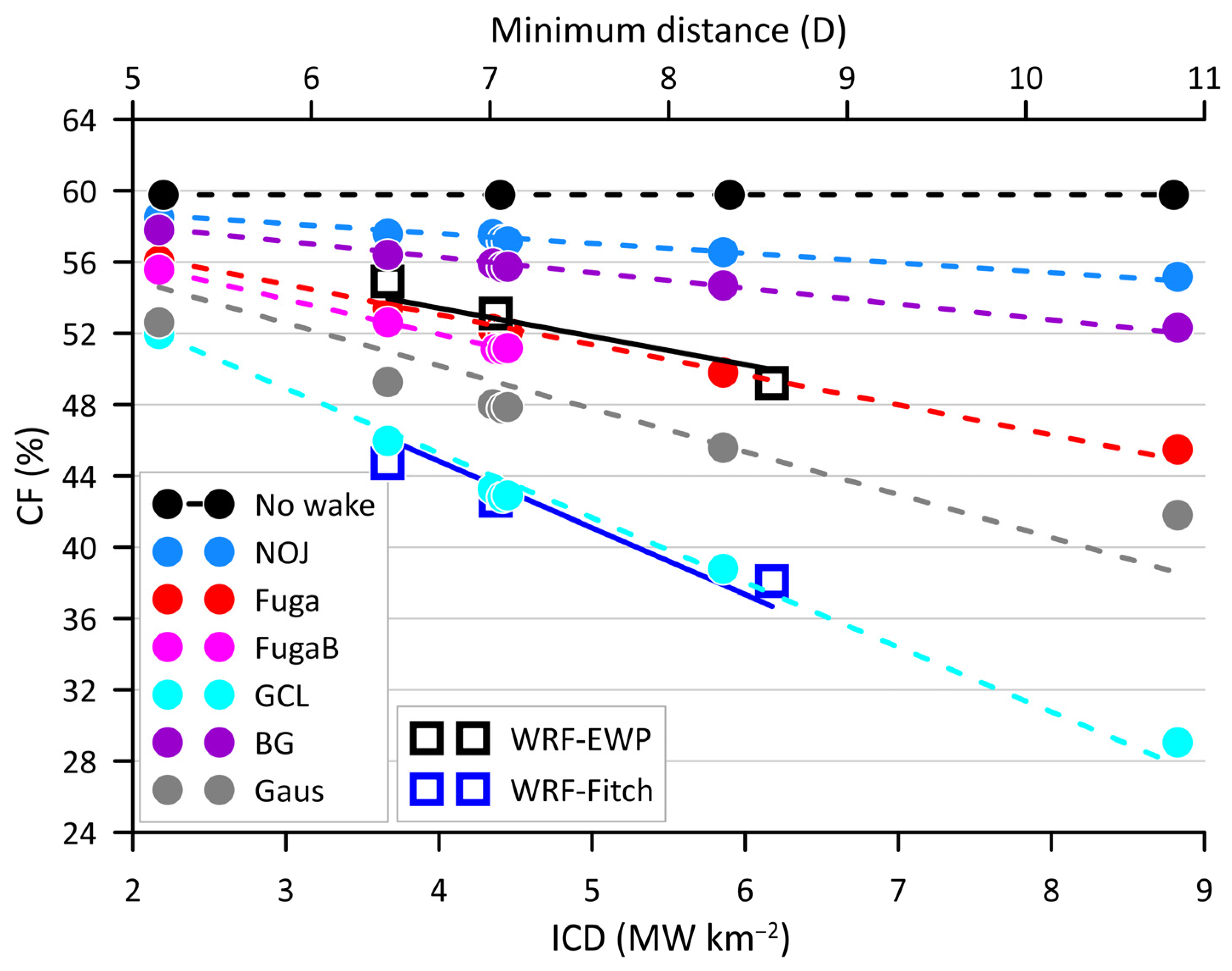
• Wake losses from the six different parameterizations span a range of 3.7 to 17.7% of AEP for the layout comprising 151 turbines at the CNTR spacing (i.e., ICD of 4.2 MW km⁻²). This is much greater than the sensitivity to the wind climate, range of 14.1–17.7% with GCL wake parameterization (HUNOW v HUERA). For comparison mean wake losses modeled with FLORIS using a WRF wind climate [78] for an ICD of 5.7 MW km⁻² are 5–6% [19].
• CF exhibit modest sensitivity to increase wind turbine spacing in the S-N direction (the cluster of points at ICD~4.5 MW km⁻² depict these different layouts; CNTR, LONG, LLNG) of up to 1.5 percentage points for some wake parameterizations.
• The change in CF with increasing ICD is most pronounced for the GCL wake parameterization. For this size of wind farm and ICD, CF (and wake loss) responses to ICD are close to linear (Figure 10). In the case of the GCL wake parameterization, linear fitting to the results implies a 2-percentage-point reduction in CF for each 1 MW km⁻² increment in ICD (

  Table 7. Mean CF for the HU LA for the CNTR layout from the different wake parameterizations for the HUNOW wind climate. The third column shows the slope coefficient (m) for linear regression fits of CF as a function of ICD from 2.0 to 8.8 MW km⁻² (see Figure 10). The linear regression equation is fitted as $\mathrm{C}\mathrm{F}=\mathrm{m}\times \mathrm{I}\mathrm{C}\mathrm{D}+\mathrm{C}\mathrm{F} \left(\mathrm{N}\mathrm{o}\mathrm{W}\mathrm{T}\right)$. Fourth column denotes the average slope of the dependency of CF on ICD from regression fits for HU and MA simulations. The column titled Estimated CF at VY is based on these regression fits, while the final column shows the modeled values for the Vineyard LA from simulations.

  Wake Parameterization	Modeled HU CF (%)	Regression Slope (m)	Average Regression Slope, m (HU and MA from Table 2)	Estimated CF at VY for ICD of 4.3 MW km−2	Modeled CF at VY for ICD of 4.3 MW km−2
  NoWT	57.8			59.7	59.7
  NOJ	55.6	−0.46	−0.51	57.48	57.70
  Fuga	53.4	−1.00	−1.34	53.80	56.39
  FugaB	52.8	−1.12	−1.52	53.03	55.71
  GCL	49.6	−1.89	−2.76	47.56	53.98
  BG	54.6	−0.70	−0.79	56.22	56.74
  Gaus	50.3	−1.50	−1.96	51.10	53.34

  ).

3.4.3. VY

When the Vineyard I wind farm is considered in isolation, due to the very large wind resource, estimated CF in the absence of wakes are close to 60% (Table 4). However, even for small offshore wind farms such as VY, the wake parameterization has a meaningful impact on the AEP, CF and wake losses (Table 4). Projected wake losses using the MAERA wind climate for a 72 wind turbine wind farm with 1.85 km spacing (7.7 D) range from 3.0% (NOJ) to 10.8% (Gaus). The latter estimate is consistent with observed wake losses from the Horns Rev I wind farm in the North Sea that uses 7 D spacing and 80 2 MW wind turbines of 12% prior to the development of the adjacent Horns Rev 2 and 3 arrays [50].

As could be expected, there is a broad similarity between the slopes m in the CF v ICD relationship for MA (Table 2) and HU simulations (Table 7) from each wake parameterization. This indicates a first CF estimate could be generated for each wake parameterization and different ICD for wind farms given the NoWT CF. Thus, an average slope is calculated (from m in Table 2 and Table 7) and the regression fits used to estimate CF for an ICD 4.3 MW km⁻² and compared with modeled CF (Table 7). Except for the GCL parameterization, CF from the linear slope estimation is within 2.5 percentage points of the modeled values. This suggests this linear regression approach may be a reasonable first estimate for smaller wind farms and more linear wake parameterizations.

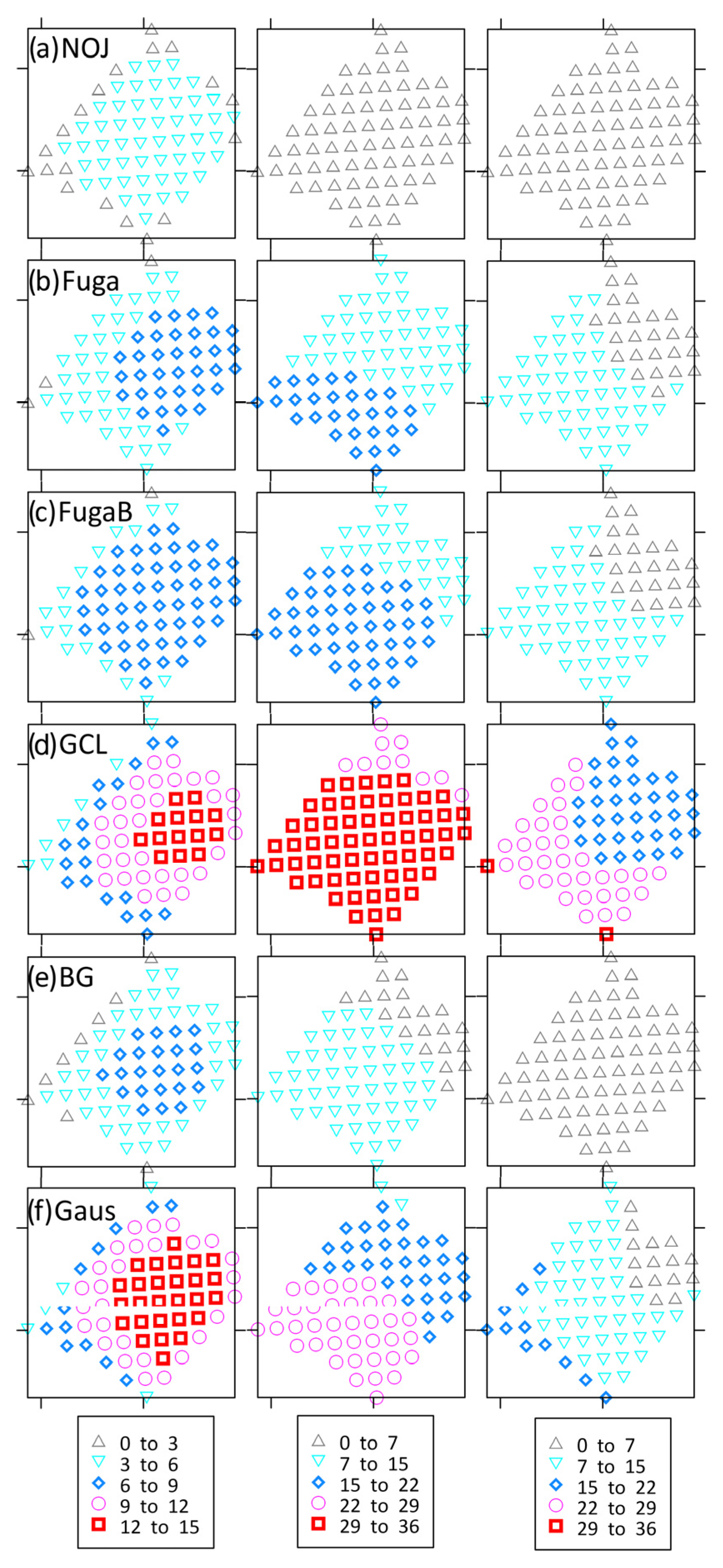
3.5. Internal vs. External Wake Effects

The VY LA within the MA cluster represents an interesting case study to consider internal and external wake losses since wind turbines within that LA will be subject to wakes from other wind turbines deployed within that LA and from adjacent LA assuming these are built out. To evaluate the impact of building out all LA around the original positions at Vineyard, six paired simulations using the MAERA wind climate are run for CNTR layouts and different wake parameterizations using (i) only the 72 Vineyard turbine locations (red wind turbine locations in Figure 2a) (ii) 1066 turbine positions in the entire MA group (black turbine locations in Figure 2a). Thus, the only difference in the predicted AEP between the paired simulations is the presence (or not) of the ‘external’ wake from the other (non-Vineyard) turbine locations in the MA group. Note the reduction by 5 wind turbines relative to earlier estimates when the MA LA cluster is populated because in this analysis the VY LA is populated first and then viable locations are found in the remainder of the adjacent LA.

The wake parameterizations indicate substantially higher wake losses when both internal and externally induced wakes are considered (

Table 8. Total Annual Energy Production (AEP), Capacity Factor (CF) and wake loss for the 72 VY turbine locations for simulations considering only internal wakes and also including external wakes (when all 1066 MA turbine locations are also present in the simulations). Simulations use the MAERA wind climate.

	VY Internal Wakes Only			VY Internal Wakes + External Wakes
Parameterization	AEP (GWh/yr)	CF(%)	Wake Loss (%)	AEP (GWh/yr)	CF (%)	Wake Loss (%)
NoWT	5659	59.8	0.0	5659	59.8	0.0
NOJ	5459	57.7	3.5	5400	57.0	4.5
Fuga	5335	56.4	5.7	4860	51.4	14.1
FugaB	5271	55.7	6.8	4782	50.6	15.4
GCL	5107	54.0	9.7	3849	40.7	31.9
BG	5368	56.7	5.1	5262	55.6	6.9
Gaus	5046	53.3	10.8	4446	47.0	21.4

and Figure 11), with the exception of NOJ (3.5% vs. 4.5%). BG gives similar but slightly higher wake losses than NOJ, particularly in the VY center (5.1% vs. 6.9%). For the remaining wake parameterizations, wake losses approximately double from internal only when including external wakes. Including external wakes triples total wake losses in simulations with the GCL parameterization (9.7% vs. 31.9%). Gaus and GCL give similar internal wake losses while Gaus predicts lower, but still substantial, total wake losses (10.8% vs. 21.4%). Fuga and FugaB give similar spatial results but with slightly higher wake losses for FugaB. Using the different wake parameterizations, not only is the overall wake loss very different but the patterns of wake losses are fundamentally changed which also has implications for dynamic wind farm control to maximize AEP.

These simulations, and other work that has indicated the growing likelihood of wake interactions between wind farms operated by different owners, may indicate a need to trade rights to consume wind resources or for dynamical control of collections of adjacent wind farms to maximize system-wide AEP and/or profits [29].

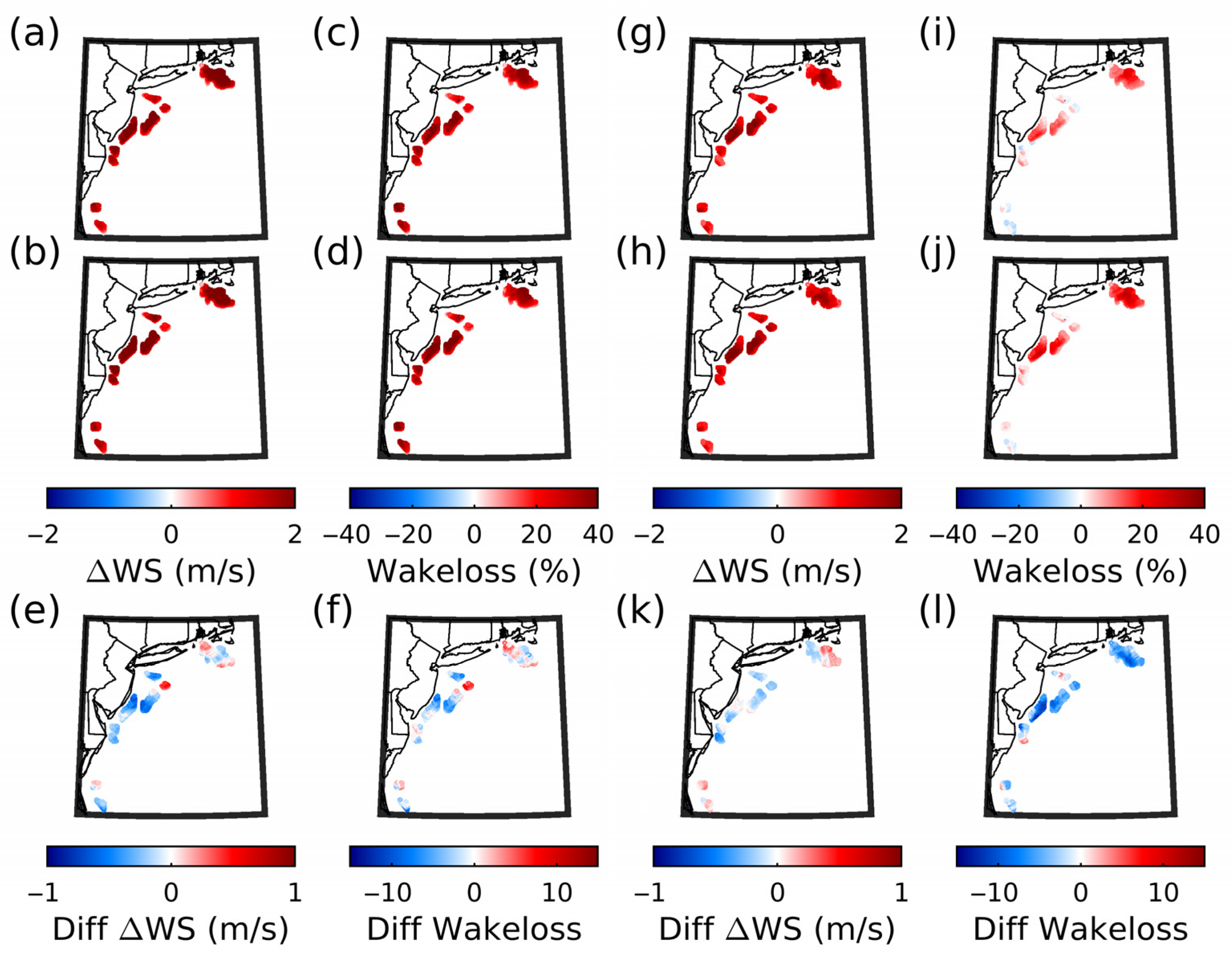
4. Results from Mesoscale Wake Modeling

The primary motivation for undertaking mesoscale simulations with WRF and COAWST is to examine whether the use of COAWST, which should better capture dynamic wind-wave coupling and sea surface temperature evolution, has a marked influence on wake losses in large offshore wind turbine arrays. The results derived from paired simulations that exclude and include the role of wind turbines (noWT vs. WT), illustrate qualitative agreement between WRF and COAWST in terms of differences in mean wind speed deficits and wake losses for the two simulation periods (Figure 12). The noWT simulations with COAWST and WRF exhibit a high degree of similarity consistent with the relatively strong synoptic scale forcing during the simulation periods. For example, freestream wind speeds at the center of the MA LA exhibit a high correlation coefficient in time (r > 0.98). This justifies use of these independent simulations to examine wake losses, but wake analyses derived using output from independent simulations should be viewed with caution because small differences in meteorological conditions (e.g., inflow wind speeds) can manifest as large differences in power production (see discussion in [30] regarding differences in power production from two different versions of WRF).

Analyses of the paired simulation show that differences (noWT–WT) in mean hub-height wind speeds can be of opposite sign to the mean wake losses due to the non-linearity of the wind turbine power curve (cf. Figure 12g,i). Time averaged (mean) wake losses exceed 20 percentage points in multiple grid cells (Figure 12) particularly during the first simulation period (August 2011) (Figure 12b,d). For this period, wake losses from WRF and COAWST are very similar (Figure 12c,d,f). The estimated system-wide wake loss is higher in WRF than COAWST by 1 percentage point (30% vs. 29%). The fraction of grid cells within the offshore LA that have wake losses of >20% is equal in the two paired simulations (86%). The magnitude of wake losses in the 260 (out of 2641 that contain WT) grid cells with maximum losses are greater in the WRF simulation (42% vs. 40%). Wake loss differences between COAWST and WRF are more pronounced in the second period (October-November 2012) and are generally larger when computed from the paired WRF simulations (Figure 12i,j,l). Mean system-wide wake losses are lower in the COAWST simulation by 5 percentage points (10% vs. 15%). The top 10th percentile of grid cell wake losses exceed 18% in the COAWST output, while those from WRF exceed 27%. Also, more LA grid cells have wake losses of >20% (70% vs. 55%) in the WRF simulation.

Although mean wake losses from the two pairs of simulations (COAWST and WRF, with and without the WFP active) exhibit high similarity (Figure 12), there are periods of disagreement. Figure 13 focusses on the MA LA and demonstrates a key and complex role for prevailing meteorology in dictating the spatial patterns and magnitude of implied wake losses. As shown, the time series of wake losses from the two model systems are highly correlated (Figure 13a,c) and exhibit a strong relationship with spatially averaged hub-height wind speeds over the MA LA. In the first simulation period freestream hub-height TKE is higher in the COAWST simulation (Figure 13b) leading to more dissipation of wakes and generally lower wake losses. Freestream TKE is also generally higher in COAWST during the second simulation period as are hub-height wind speeds (Figure 13d). The period of largest discrepancy in wake losses (later in the simulation period, Figure 13c) is characterized by both higher wind speeds in COAWST and higher TKE which lead to lower thrust coefficients (lower wake generation) and greater wake dissipation in COAWST (i.e., ΔWakeloss shown in Figure 13b,d is negative indicating larger wake losses from WRF).

Differences in system-wide wake losses (1 or 5 percentage points) from COAWST v WRF for these two simulation periods are substantial in terms of system-wide AEP given the large, simulated IC in the CNTR layout of ~38 GW. However, differences in wakes losses from COAWST v WRF are smaller than the differences in climatological estimates of system-wide wake losses computed using WRF simulations with the EWP or Fitch WFP (>10 percentage points) [30]. Nevertheless, further work is merited to explore the causes of wake loss dependence on the mesoscale model system (COAWST vs. WRF), and to examine the degree to which these differences are dependent on the precise model configuration used and prevailing meteorological conditions.

5. Discussion

As noted in the introduction, the magnitude of wake losses in much smaller, isolated offshore wind farms (with installed capacities of ~40–200 MW) lie in the range of 10–23% [50]. However, planned offshore developments are likely to have larger spatial extent and installed capacities (600 MW to 3 GW) and to increasingly operate in the wind shadow of neighboring wind farms [30]. The synthesis of the range of modeled Annual Energy Production (AEP), Capacity Factor (CF) and wake losses based on simulations of the US offshore wind energy lease areas (LA) with a range of platforms and assumptions shown in

Table 9. AEP, CF and wake loss calculations for simulations performed on different platforms (WRF or PyWake), or using different wind climates, wake/wind farm parameterizations, and/or ICD. Color shading denotes the LA (All east coast LA = gold; MA = blue; VY = gray; HU (west coast) = orange). The cell boundary has a double border to denote the property being varied which is also shown in bold font; e.g., wind farm/wake parameterization, ICD, wind climate and the corresponding results are shown in cells with a red outline. The range of AEP, CF or wake losses from different simulations is shown in italics.

LA (Section)	Platform	Wind Climate/Source of LBC for Mesoscale	Wind Farm/Wake Parameterization	Number of Turbines #	ICD (MW/km2)	AEP (GWh/y)	Range of AEP (Waked) (%)	CF (%)	Range of CF (Waked) (Percentage Points)	Wake Losses (%)	Wake Range (Percentage Points)
All (3.1)	PyWake	NJERA	NoWT, NOJ, Fuga	2617	4.3	191,067, 182,682, 169,756	7.1	55.6, 53.1, 49.4	3.8	0, 4.4, 11.2	6.8
All (3.1)	WRF	ERA5	EWP, Fitch [30]	1922	4.3			53.2, 42.6	10.6
All (3.1)	WRF	ERA5	EWP [30]	1604–2598	3.5–6.0			54.9– 49.7	5.2	11–19	8
All (3.1)	WRF	ERA5	Fitch [30]	1604–2598	3.5– 6.0			44.8–38.7	6.1	27–37	10
MA (3.2.1)	WRF	ERA5	EWP [30]	1073– 1485	4.3, 6.0			53.1, 49.2	3.9
MA (3.2.1)	WRF	ERA5	Fitch [30]	1073– 1485	4.3, 6.0			42.6 38.1	4.5
MA (3.2.1)	PyWake	MAERA	NOJ	532–2162	2.2–8.8	40,891–156,727	73.9	58.5–55.2	3.3	2.1– 7.7	5.6
MA (3.2.1)	Py-Wake	MAERA	Fuga	532–2162	2.2–8.8	39,194–129,200	69.7	56.1 45.5	10.6	6.3– 23.9	17.6
HU (3.2.2)	Py-Wake	Recon	NOJ	78– 306	2.2–8.6	6227–22,899	72.8	56.6–53.7	2.9	2.2– 8.4	6.2
HU (3.2.2)	Py-Wake	Recon	Fuga	78– 306	2.2–8.6	6078–20,358	70.1	55.5–48.9	6.6	4.6– 18.6	14.0
VY (3.3.1)	Py-Wake	VYERA, VYNOW, MAERA	NoWT	72	4.3	5663, 5695, 5665	0.5	59.9, 60.2, 59.8	0.4	-	-
HU (3.3.2)	Py-Wake	HUERA, HUNOW, Recon	NoWT	151	4.2	10,444, 11,459, 12,337	18.1	52.0, 61.1, 61.4	9.4	-	-
MA (3.4.1)	PyWake	MAERA	NOJ, Fuga, GCL, BG, Gaus	1066	4.3	60,593–80,624	24.8	43.3–57.6	14.3	3.7– 27.6	23.9
VY (3.4.2)	PyWake	VYERA	NOJ, Fuga, FugaB, GCL, BG, Gaus	72	4.3	5049– 6159	18.0	53.4–57.8	4.4	3.5– 10.8	7.3
HU (3.4.3)	PyWake	HUNOW	NOJ, Fuga, FugaB, GCL, BG, Gaus	151	4.2	9845–11,040	10.8	49.6–55.6	6.0	3.7– 12.1	8.4
VY (3.5)	PyWake	MAERA	NOJ, Fuga, GCL, BG, Gaus	72	4.3	5046– 5459	7.7	53.3–57.7	4.4	3.5– 10.8	7.3
VY in MA (3.5)	PyWake	MAERA	NOJ, Fuga, GCL, BG, Gaus	72 of 1066	4.3	3849– 5400	28.7	40.7–57.1	17.2	4.5– 31.9	27.4

indicates wake losses for this next generation of offshore wind farms may greatly exceed these historical values. Wake losses may exceed 30% in some situations and thus will play an increasing role in dictating LCoE.

Results summarized in Table 9 indicate:

(1)

Use of wind climates from different sources has only a moderate effect on modeled AEP, CF and wake losses for the LA considered herein and the range of engineering wake models. Along the US east coast, the range of AEP or CF arising from use of output data the ERA5 reanalysis or NOW-23 is small. For example, at the VY LA use of ERA5 or NOW-23 gives AEP projections that lie within ~1% of each other. However, at the HU LA projected AEP from the Recon dataset averages 6 percentage points higher than when NOW-23 data is used and differs by over 16 percentage points from simulations based on HUERA. Thus, there would be utility in performing additional measurements to validate model output from ERA5 [42] and NOW-23 [44]. However, the use of wind climates from these sources does not appear to be a dominant source of uncertainty in AEP projections at least for offshore wind energy LA along the US east coast.

(2)

Increasing ICD leads to higher AEP, but also results in increased wake losses, which can markedly reduce CF (Figure 6 and Figure 10). This trade-off is important for developers, who must balance higher energy production with additional CAPEX costs and the risk of additional fatigue loading and potentially enhanced OPEX.

(3)

CF vary considerably across the range of microscale wake engineering models and discrepancies increase with wind farm size and ICD. For the MA LA (Section 3.2.1), the range of simulated wake losses using Fuga is 17.9 percentage points for ICD increasing from 2.2 to 8.8 MW km⁻². This is a smaller range than simulated with different wake parameterizations (Section 3.2.2) of 23.9 percentage points. Generally, the GCL wake parameterization yields lowest CF and exhibits the strongest dependence on ICD (see Figure 6 and Table 2). NOJ predicts the lowest wake losses and thus highest AEP/CF. FugaB is the only wake parameterization to include blockage but also requires the most computer memory and thus it was not possible to explore the full range of ICD for this wake parameterization even on a system with 500 GB of RAM.

(4)

Some studies have shown reasonable agreement between WRF and engineering models simulations in terms of wind speed deficits in case studies [23,26,80]. For the US east coast, climatological CF is lowest from the Fitch WFP within WRF and based on microscale modeling with GCL. Mean CF from WRF-Fitch and the GCL wake parameterization also exhibit a similar dependence on ICD. Conversely, climatological CF from WRF-EWP is considerably higher and are most consistent with Fuga in absolute terms and with respect to the dependence on ICD.

(5)

Increasing ICD from 2.2 to 8.8 MW km⁻² (i.e., quadrupling the number of wind turbines deployed in the largest wind energy lease area cluster that covers 3673 km²) increases AEP by a factor of less than four indicating the emergence of an increasingly large deep array effect where power production from wind turbines in the center of the array is substantially compromised by wake losses. AEP increases by a factor of 2.3–3.8 depending on the wake parameterization, with the GCL wake parameterization showing lowest AEP gain with increasing ICD.

(6)

Even for very large LA clusters, CF from most wake parameterizations scale approximately linearly with ICD for ICD of 2.2 to 8.8 MW km⁻². Within this likely range of ICD, a simple scaling analysis extrapolating from the noWT CF that depends solely on the wind climate can provide preliminary projections of AEP without the need for numerous detailed simulations. However, we note that the Gaus wake model, that is trained on observations from smaller offshore wind farms, exhibits the most non-linear response to ICD changes. Further, use of these fits of CF to ICD in out-of-sample contexts (e.g., other wind climates) is not recommended.

Most comparisons of engineering wake models with measurements show that models underestimate wake loss magnitudes [76,81] and farm-to-farm wake interactions [23,26]. Thus, it is likely that actual CF realized from the next generation of offshore wind farms are likely to be closer to those predicted from parameterizations that yield larger wake losses (GCL, Gaus and FugaB). Without further validation using SCADA data from offshore wind farms, Gaus may represent the optimal choice [61,63] due to the following considerations: (i) It was developed using operational data from offshore wind farms, although they are of smaller dimensions that those under current consideration, (ii) the results, in terms of wake losses, are midway between the two WRF WFP and are also close to those from FugaB for simulations with up to 1000 wind turbines deployed at an ICD of approximately 4.5 MW km⁻² and (iii) it is not the most computationally expensive option.

Naturally, results presented herein do not sample the full range of possibilities in terms of wake expansion coefficients or the turbulence intensity (GCL) and wake superposition. Default values were used in this analysis. The model resolution has limited impact in Engineering models but is important in WRF [82].

6. Conclusions

Offshore wind energy development lease areas (LA) along the US east coast will, if realized, constitute offshore arrays of unprecedented spatial scale and total IC. For example, if the LA south of the US states of Massachusetts and Rhode Island were fully built out with 13 MW wind turbines at a 1.85 km spacing, the IC would be 14 GW, several times larger than the largest offshore wind farm currently operating. Wind turbines in these large arrays predominantly operate in disturbed conditions due to the wakes generated by upstream wind turbines. The resulting wake losses are a major source of uncertainty in economic planning and have tremendous relevance in the context of continuing price pressure. Uncertainty in wake losses of the order described in this manuscript can result in income differences in millions of dollars each year.

The impact on AEP, CF and wake loss predictions for large offshore wind farms that derives from use of different layouts (ICD in the range of 2.2 to 8.8 MW km⁻²), meteorological datasets and wake parameterizations is quantified. Both the microscale and mesoscale simulations indicate the range of simulated CF that derives from the wake/wind farm parameterization used is larger than the range generated using different wind climates and can be greater than the range of CF generated by quadrupling ICD. Differences in projections made using different wake and wind farm parameterizations increase as larger wind farms or clusters are simulated and there is a strong dependence on ICD. For example, while the GCL wake parameterization and Fitch WFP indicate an approximately 3 percentage point reduction in CF for each 1 MW km⁻² increase in ICD, simulations with Gaus and the EWP WFP indicate only an ~2 percentage point reduction in CF for each 1 MW km⁻² increase in ICD. In addition to wind farm average wake losses, spatial patterns of wake losses are also highly dependent on the wake parameterization selected. This could impact the effectiveness and the ability to detect the efficiency of control strategies (e.g., wake steering) that seek to improve performance by a few percentage points [83], particularly in large wind farms. The difference in AEP projections from the WRF mesoscale model that employ different WFPs are larger than those that result from use of more comprehensive treatment of wind-wave-ocean coupling.

As mentioned in the introduction, the size and scale of offshore wind farms in areas such as the North Sea, combined with relatively small areas available for current wind energy technology inevitably means that discussions are needed if wind farms are built upwind of existing developments [84]. As shown, wake losses from a modestly sized wind farm with a footprint of ~306 km⁻² are doubled in simulations wherein LA around it are built out. Accurate assessment of internal and externally generated wakes and wake losses to each wind farm are important to economics/project financing, optimization of layouts and operation of existing and new offshore wind energy developments. Accordingly, a major effort is needed to validate and improve wake models and WFP modules for large offshore wind farms. Individual offshore wind farm developers are performing these analyses using data from their own operating wind farms [63] or making case study data available. However, an open database that contains climatologically relevant SCADA data including critical parameters such as power output, operating status, yaw angle and inflow wind speed from individual turbines across a wide array of meteorological conditions from increasingly large offshore wind farms would allow wider participation, ensure more generalizability of findings and benefit the entire industry.

References

1. Global Wind Report 2025; The Global Wind Energy Council: Brussels, Belgium, 2025; p. 108. Available online: https://www.gwec.net/reports/globalwindreport (accessed on 23 April 2025).
2. Buljan, A. Half of Global Operational Offshore Wind Capacity in China Industry. Available online: https://www.offshorewind.biz/2025/02/07/half-of-global-operational-offshore-wind-capacity-in-china/ (accessed on 7 February 2025).
3. Latest Wind Energy Data for Europe; WindEurope: Brussels, Belgium, 2024; p. 36. Available online: https://windeurope.org/intelligence-platform/product/latest-wind-energy-data-for-europe-autumn-2024/ (accessed on 9 January 2025).
4. Global Wind Energy Council Global Offshore Wind Report 2024; The Global Wind Energy Council: Brussels, Belgium, 2024; p. 156. Available online: https://www.gwec.net/reports/globaloffshorewindreport/2024 (accessed on 31 December 2024).
5. Wind Energy in Europe Trends and Statistics 2019; WindEurope: Brussels, Belgium, 2020; p. 24. Available online: https://windeurope.org/wp-content/uploads/files/about-wind/statistics/WindEurope-Annual-Statistics-2019.pdf (accessed on 27 February 2020).
6. Offshore Wind Energy 2024 Statistics; WindEurope: Brussels, Belgium, 2025; p. 49. Available online: https://windeurope.org/intelligence-platform/reports/ (accessed on 11 June 2025).
7. Pryor, S.C.; Barthelmie, R.J. Wind shadows impact planning of large offshore wind farms. Appl. Energy 2024, 359, 122755. [Google Scholar] [CrossRef]
8. Barthelmie, R.J.; Larsen, G.C.; Pryor, S.C. Modeling Annual Electricity Production and Levelized Cost of Energy from the US East Coast Offshore Wind Energy Lease Areas. Energies 2023, 16, 4550. [Google Scholar] [CrossRef]
9. Tjaberings, J.; Fazi, S.; Ursavas, E. Evaluating operational strategies for the installation of offshore wind turbine substructures. Renew. Sustain. Energy Rev. 2022, 170, 112951. [Google Scholar] [CrossRef]
10. Virtanen, E.A.; Lappalainen, J.; Nurmi, M.; Viitasalo, M.; Tikanmäki, M.; Heinonen, J.; Atlaskin, E.; Kallasvuo, M.; Tikkanen, H.; Moilanen, A. Balancing profitability of energy production, societal impacts and biodiversity in offshore wind farm design. Renew. Sustain. Energy Rev. 2022, 158, 112087. [Google Scholar] [CrossRef]
11. Hansen, T.A.; Wilson, E.J.; Fitts, J.P.; Jansen, M.; Beiter, P.; Steffen, B.; Xu, B.; Guillet, J.; Münster, M.; Kitzing, L. Five grand challenges of offshore wind financing in the United States. Energy Res. Soc. Sci. 2024, 107, 103329. [Google Scholar] [CrossRef]
12. Ambrose, J. What Went Wrong at UK Government’s Offshore Wind Auction? The Guardian: London, UK, 2023; Available online: https://www.theguardian.com/environment/2023/sep/08/what-went-wrong-at-uk-governments-offshore-wind-auction (accessed on 8 September 2023).
13. Buljan, A. US Cancels Second Gulf of Mexico Offshore Wind Lease Sale; offshoreWIND.biz: Rotterdam, The Netherlands, 2024; Available online: https://www.offshorewind.biz/2024/07/26/us-cancels-second-gulf-of-mexico-offshore-wind-lease-sale/ (accessed on 25 April 2025).
14. No Offshore Bids in Denmark—Disappointing but Sadly Not Surprising; WindEurope: Brussels, Belgium, 2024; Available online: https://windeurope.org/newsroom/press-releases/no-offshore-bids-in-denmark-disappointing-but-sadly-not-surprising/ (accessed on 7 September 2024).
15. Jordan, D. Nine Offshore Wind Farm Projects Awarded in UK Auction. BBC News, 3 September 2024. Available online: https://www.bbc.com/news/articles/c86ldzve4neo (accessed on 3 September 2024).
16. Borrmann, R.; Rehfeldt, K.; Wallasch, A.K.; Lüers, S. Capacity Densities of European Offshore Wind Farms; SP18004A1; Deutsche Windguard GmbH: Hamburg, Germany, 2018; p. 86. Available online: https://www.msp-platform.eu/practices/capacity-densities-european-offshore-wind-farms (accessed on 20 January 2021).
17. Pryor, S.C.; Barthelmie, R.J.; Shepherd, T.J. Wind power production from very large offshore wind farms. Joule 2021, 5, 2663–2686. [Google Scholar] [CrossRef]
18. Barthelmie, R.J.; Frandsen, S.T.; Nielsen, N.M.; Pryor, S.C.; Rethore, P.E.; Jørgensen, H.E. Modelling and measurements of power losses and turbulence intensity in wind turbine wakes at Middelgrunden offshore wind farm. Wind Energy 2007, 10, 217–228. [Google Scholar] [CrossRef]
19. Cooperman, A.; Duffy, P.; Hall, M.; Lozon, E.; Shields, M.; Musial, W. Assessment of Offshore Wind Energy Leasing Areas for Humboldt and Morro Bay Wind Energy Areas, California; NREL/TP-5000-82341; National Renewable Energy Laboratory (NREL): Golden, CO, USA, 2022; p. 85. Available online: https://www.nrel.gov/docs/fy22osti/82341.pdf (accessed on 2 May 2023).
20. Draft Construction and Operations Plan Volume I Vineyard Wind Project; Vineyard Wind LLC: New Bedford, MA, USA, 2020; p. 27. Available online: https://www.boem.gov/sites/default/files/documents/renewable-energy/Vineyard-Wind-COP-Volume-III-Section-4.pdf (accessed on 31 December 2024).
21. Richard, C. Vineyard Wind Secures Levelised Cost of $65/MWh; Windpower Monthly: London, UK, 2018; Available online: https://www.windpowermonthly.com/article/1489414/vineyard-wind-secures-levelised-cost-65-mwh (accessed on 7 September 2024).
22. Sebastiani, A.; Castellani, F.; Crasto, G.; Segalini, A. Data analysis and simulation of the Lillgrund wind farm. Wind Energy 2021, 24, 634–648. [Google Scholar] [CrossRef]
23. Fischereit, J.; Schaldemose Hansen, K.; Larsén, X.G.; van der Laan, M.P.; Réthoré, P.E.; Murcia Leon, J.P. Comparing and validating intra-farm and farm-to-farm wakes across different mesoscale and high-resolution wake models. Wind Energy Sci. 2022, 7, 1069–1091. [Google Scholar] [CrossRef]
24. Badger, M.; Pena Diaz, A.; Hahmann, A.N.; Mouche, A.; Hasager, C.B. Extrapolating satellite winds to turbine operating heights. J. Appl. Meteorol. Climatol. 2016, 55, 975–991. [Google Scholar] [CrossRef]
25. Schneemann, J.; Rott, A.; Dörenkämper, M.; Steinfeld, G.; Kühn, M. Cluster wakes impact on a far-distant offshore wind farm’s power. Wind Energy Sci. 2020, 5, 29–49. [Google Scholar] [CrossRef]
26. Cañadillas, B.; Foreman, R.; Barth, V.; Siedersleben, S.; Lampert, A.; Platis, A.; Djath, B.; Schulz-Stellenfleth, J.; Bange, J.; Emeis, S.; et al. Offshore wind farm wake recovery: Airborne measurements and its representation in engineering models. Wind Energy 2020, 23, 1249–1265. [Google Scholar] [CrossRef]
27. Nygaard, N.G.; Newcombe, A.C. Wake behind an offshore wind farm observed with dual-Doppler radars. J. Phys. Conf. Ser. 2018, 1037. [Google Scholar] [CrossRef]
28. Howland, M.F.; Quesada, J.B.; Martínez, J.J.P.; Larrañaga, F.P.; Yadav, N.; Chawla, J.S.; Sivaram, V.; Dabiri, J.O. Collective wind farm operation based on a predictive model increases utility-scale energy production. Nat. Energy 2022, 7, 818–827. [Google Scholar] [CrossRef]
29. Kenis, M.; Lanzilao, L.; Bruninx, K.; Meyers, J.; Delarue, E. Trading rights to consume wind in presence of farm-farm interactions. Joule 2023, 7, 1394–1398. [Google Scholar] [CrossRef]
30. Pryor, S.C.; Barthelmie, R.J. Power Production, Inter- and Intra-Array Wake Losses from the U.S. East Coast Offshore Wind Energy Lease Areas. Energies 2024, 17, 1063. [Google Scholar] [CrossRef]
31. Thomas, J.J.; Baker, N.F.; Malisani, P.; Quaeghebeur, E.; Sanchez Perez-Moreno, S.; Jasa, J.; Bay, C.; Tilli, F.; Bieniek, D.; Robinson, N.; et al. A comparison of eight optimization methods applied to a wind farm layout optimization problem. Wind Energ. Sci. 2023, 8, 865–891. [Google Scholar] [CrossRef]
32. Warder, S.C.; Piggott, M.D. The future of offshore wind power production: Wake and climate impacts. Appl. Energy 2025, 380, 124956. [Google Scholar] [CrossRef]
33. Foody, R.; Coburn, J.; Aird, J.A.; Barthelmie, R.J.; Pryor, S.C. Quantitative comparison of power production and power quality onshore and offshore: A case study from the eastern United States. Wind Energy Sci. 2024, 9, 263–280. [Google Scholar] [CrossRef]
34. U.S. Bureau of Ocean Energy Management. Renewable Energy GIS Data. 2024. Available online: https://www.boem.gov/renewable-energy/mapping-and-data/renewable-energy-gis-data (accessed on 18 September 2024).
35. Barthelmie, R.J.; Dantuono, K.; Renner, E.; Letson, F.; Pryor, S.C. Extreme wind and waves in U.S. east coast offshore wind energy lease areas. Energies 2021, 14, 1053. [Google Scholar] [CrossRef]
36. renews.BIZ. Uniform Turbine Layout Touted for NE US Offshore Wind. 2019. Available online: https://renews.biz/56505/uniform-turbine-layout-touted-for-ne-offshore-wind/ (accessed on 21 October 2021).
37. Ahmed, Z. Top 12 Biggest Offshore Wind Farms in The World. Available online: https://www.marineinsight.com/know-more/biggest-offshore-wind-farms/ (accessed on 12 July 2024).
38. Bureau of Ocean Energy Management. Final Environmental Assessment. Commercial Wind Lease and Grant Issuance and Site Assessment Activities on the Pacific Outer Continental Shelf Humboldt Wind Energy Area, California; Bureau of Ocean Energy Management: Washington, DC, USA, 2022; p. 101. Available online: https://www.boem.gov/sites/default/files/documents/renewable-energy/state-activities/Humboldt-EA.pdf (accessed on 17 January 2025).
39. Gaertner, E.; Rinker, J.; Sethuraman, L.; Zahle, Z.; Anderson, B.; Barter, G.; Abbas, B.; Meng, F.; Bortolotti, F.; Skrzypinski, W.; et al. Definition of the IEA 15-Megawatt Offshore Reference Wind Turbine; NREL/TP-5000-75698; National Renewable Energy Laboratory: Golden, CO, USA, 2020. Available online: https://www.nrel.gov/docs/fy20osti/75698.pdf (accessed on 5 November 2020).
40. von Brandis, A.; Centurelli, G.; Schmidt, J.; Vollmer, L.; Djath, B.; Dörenkämper, M. An investigation of spatial wind direction variability and its consideration in engineering models. Wind Energy Sci. 2023, 8, 589–606. [Google Scholar] [CrossRef]
41. Simley, E.; Fleming, P.; King, J.; Sinner, M. Wake Steering Wind Farm Control With Preview Wind Direction Information. In 2021 American Control Conference; IEEE: New York, NY, USA, 2021; pp. 1783–1789. [Google Scholar] [CrossRef]
42. Hersbach, H.; Bell, B.; Berrisford, P.; Hirahara, S.; Horányi, A.; Muñoz-Sabater, J.; Nicolas, J.; Peubey, C.; Radu, R.; Schepers, D.; et al. The ERA5 global reanalysis. Q. J. R. Meteorol. Soc. 2020, 146, 1999–2049. [Google Scholar] [CrossRef]
43. Krishnamurthy, R.; García Medina, G.; Gaudet, B.; Gustafson, W.I., Jr.; Kassianov, E.I.; Liu, J.; Newsom, R.K.; Sheridan, L.M.; Mahon, A.M. Year-long Buoy-Based Observations of the Air–Sea Transition Zone off the U.S. West Coast. Earth Syst. Sci. Data 2023, 15, 5667–5699. [Google Scholar] [CrossRef]
44. Bodini, N.; Optis, M.; Rossol, M.; Rybchuk, A.; Lundquist, J.K.; Rosencrans, D. 2023 National Offshore Wind Dataset; National Renewable Energy Laboratory: Golden, CO, USA, 2024; Available online: https://data.openei.org/submissions/4500 (accessed on 9 December 2024). [CrossRef]
45. Rogers, A.; Rogers, J.; Manwell, J.F. Comparison of the performance of four measure-correlate-predict algorithms. J. Wind Eng. Ind. Aerodyn. 2005, 93, 243–264. [Google Scholar] [CrossRef]
46. National Data Buoy Center Station 46022 (LLNR 500). 2024. Available online: https://www.ndbc.noaa.gov/station_page.php?station=46022 (accessed on 17 January 2025).
47. Barthelmie, R.J. Evaluating the impact of wind induced roughness change and tidal range on extrapolation of offshore vertical wind speed profiles. Wind Energy 2001, 4, 99–105. [Google Scholar] [CrossRef]
48. International Electrotechnical Commission. International Standard, IEC61400 Wind Turbines Part 3-1: Design Requirements for Fixed Offshore Wind Turbines, Edition 1.0 2019-04; IEC, FDIS: Geneva, Switzerland, 2019; p. 314. [Google Scholar]
49. Pryor, S.C.; Nielsen, M.; Barthelmie, R.J.; Mann, J. Can satellite sampling of offshore wind speeds realistically represent wind speed distributions? Part II: Quantifying uncertainties associated with sampling strategy and distribution fitting methods. J. Appl. Meteorol. 2004, 43, 739–750. [Google Scholar] [CrossRef]
50. Barthelmie, R.J.; Pryor, S.C.; Frandsen, S.T.; Hansen, K.; Schepers, J.G.; Rados, K.; Schlez, W.; Neubert, A.; Jensen, L.E.; Neckelmann, S. Quantifying the impact of wind turbine wakes on power output at offshore wind farms. J. Atmos. Ocean. Technol. 2010, 27, 1302–1317. [Google Scholar] [CrossRef]
51. Göçmen, T.; Laan, P.v.d.; Réthoré, P.-E.; Diaz, A.P.; Larsen, G.C.; Ott, S. Wind turbine wake models developed at the technical university of Denmark: A review. Renew. Sustain. Energy Rev. 2016, 60, 752–769. [Google Scholar] [CrossRef]
52. Nygaard, N.G. Wakes in very large wind farms and the effect of neighbouring wind farms. J. Phys. Conf. Ser. 2014, 524, 012162. [Google Scholar] [CrossRef]
53. Christiansen, M.B.; Hasager, C. Wake effects of large offshore wind farms identified from satellite SAR. Remote Sens. Environ. 2005, 98, 251–268. [Google Scholar] [CrossRef]
54. Pedersen, M.M.; van der Laan, P.; Friis-Møller, M.; Rinker, J.; Réthoré, P.-E. DTUWindEnergy/PyWake: PyWake (Version v1.0.10); Zenodo: Geneva, Switzerland, 2019. [Google Scholar] [CrossRef]
55. Jensen, N.O. A Note on Wind Turbine Interaction; Risø-M-2411; Risø National Laboratory: Roskilde, Denmark, 1983; p. 16. Available online: https://orbit.dtu.dk/en/publications/a-note-on-wind-generator-interaction (accessed on 5 December 2017).
56. Katic, I.; Højstrup, J.; Jensen, N.O. A simple model for cluster efficiency. In Proceedings of the European Wind Energy Association, Rome, Italy, 7–9 October 1986; pp. 407–409. [Google Scholar]
57. Troen, I.; Petersen, E.L. European Wind Atlas; Risø National Laboratory: Roskilde, Denmark, 1989; p. 656. Available online: http://orbit.dtu.dk/files/112135732/European_Wind_Atlas.pdf (accessed on 31 December 2024).
58. Ott, S.; Nielsen, M. Developments of the Offshore Wind Turbine Wake Model Fuga; DTU Wind Energy: Roskilde, Denmark, 2014; p. 22. ISBN 978-87-92896-81-0. Available online: https://orbit.dtu.dk/en/publications/developments-of-the-offshore-wind-turbine-wake-model-fuga (accessed on 27 September 2021).
59. Ott, S.; Berg, J.; Nielsen, M. Linearised CFD Models for Wakes; Risoe-R-1772 (EN); DTU: Roskilde, Denmark, 2011; Available online: https://orbit.dtu.dk/en/publications/linearised-cfd-models-for-wakes(c29803f3-a1eb-45ab-b73f-ede444928477).html (accessed on 26 July 2019).
60. Meyer Forsting, A.; Troldborg, N.; Gaunaa, M. The flow upstream of a row of aligned wind turbine rotors and its effect on power production. Wind Energy 2017, 20, 63–77. [Google Scholar] [CrossRef]
61. Pedersen, J.G.; Svensson, E.; Poulsen, L.; Nygaard, N.G. Turbulence Optimized Park model with Gaussian wake profile. J. Phys. Conf. Ser. 2022, 2265, 022063. [Google Scholar] [CrossRef]
62. Orsted. 2022. Available online: https://github.com/OrstedRD/TurbOPark (accessed on 3 May 2023).
63. Nygaard, N.G.; Poulsen, L.; Svensson, E.; Pedersen, J.G. Large-scale benchmarking of wake models for offshore wind farms. J. Phys. Conf. Ser. 2022, 2265, 022008. [Google Scholar] [CrossRef]
64. Bastankhah, M.; Porté-Agel, F. A new analytical model for wind-turbine wakes. Renew. Energy 2016, 70, 116–123. [Google Scholar] [CrossRef]
65. Larsen, G.C. A Simple Stationary Semi-Analytical Wake Model. Risø National Laboratory for Sustainable Energy, Technical University of Denmark. Denmark. Forskningscenter Risoe. Risoe-R No. 1713(EN). 2009. Available online: https://orbit.dtu.dk/en/publications/a-simple-stationary-semi-analytical-wake-model (accessed on 24 June 2024).
66. Skamarock, W.C.; Klemp, J.B.; Dudhia, J.; Gill, D.O.; Barker, D.M.; Wang, W.; Powers, J.G. A Description of the Advanced Research WRF Version 2; Note NCAR/TN-468+STR; NCAR Tech: Boulder, CO, USA, 2005; p. 88. [Google Scholar]
67. Thompson, K.B.; Barthelmie, R.J.; Pryor, S.C. Hurricane impacts in the United States East Coast offshore wind energy lease areas. Wind Energy Sci. Discuss. 2025, Preprint wes-2025-37. [Google Scholar] [CrossRef]
68. Fitch, A.C.; Olson, J.B.; Lundquist, J.K. Parameterization of Wind Farms in Climate Models. J. Clim. 2013, 26, 6439–6458. [Google Scholar] [CrossRef]
69. Fitch, A.C.; Olson, J.B.; Lundquist, J.K.; Dudhia, J.; Gupta, A.K.; Michalakes, J.; Barstad, I. Local and Mesoscale Impacts of Wind Farms as Parameterized in a Mesoscale NWP Model. Mon. Weather Rev. 2012, 140, 3017–3038. [Google Scholar] [CrossRef]
70. Archer, C.L.; Wu, S.; Ma, Y.; Jiminez, P.A. Two Corrections for Turbulent Kinetic Energy Generated by Wind Farms in the WRF Model. Mon. Weather Rev. 2020, 148, 4823–4835. [Google Scholar] [CrossRef]
71. Volker, P.J.H.; Badger, J.; Hahmann, A.N.; Ott, S. The Explicit Wake Parametrisation V1.0: A wind farm parametrisation in the mesoscale model WRF. Geosci. Model Dev. 2015, 8, 3481–3522. [Google Scholar] [CrossRef]
72. Pryor, S.C.; Shepherd, T.; Volker, P.; Hahmann, A.; Barthelmie, R.J. ‘Wind theft’ from onshore arrays: Sensitivity to wind farm parameterization and resolution. J. Appl. Meteorol. Climatol. 2020, 59, 153–174. [Google Scholar] [CrossRef]
73. Porchetta, S.; Muñoz-Esparza, D.; Munters, W.; van Beeck, J.; van Lipzig, N. Impact of ocean waves on offshore wind farm power production. Renew. Energy 2021, 180, 1179–1193. [Google Scholar] [CrossRef]
74. Warner, J.C.; Armstrong, B.; He, R.; Zambon, J.B. Development of a Coupled Ocean–Atmosphere–Wave–Sediment Transport (COAWST) Modeling System. Ocean Model. 2010, 35, 230–244. [Google Scholar] [CrossRef]
75. U.S. Energy Information Administration. Electricity Consumption in the United States Was About 4 Trillion Kilowatthours (kWh) in 2022. 2023. Available online: https://www.eia.gov/energyexplained/electricity/use-of-electricity.php (accessed on 16 September 2024).
76. Barthelmie, R.J.; Jensen, L.E. Evaluation of wind farm efficiency and wind turbine wakes at the Nysted offshore wind farm. Wind Energy 2010, 13, 573–586. [Google Scholar] [CrossRef]
77. Irwin, J.S. A theoretical variation of the wind profile power-law exponent as a function of surface roughness and stability. Atmos. Environ. 1979, 13, 191–194. [Google Scholar] [CrossRef]
78. Optis, M.; Rybchuk, O.; Nicola, B.; Rossol, M.; Musial, W. Offshore Wind Resource Assessment for the California Pacific Outer Continental Shelf; NREL/TP-5000-77642; National Renewable Energy Laboratory (NREL): Golden, CO, USA, 2020. [Google Scholar] [CrossRef]
79. Bodini, N.; Rybchuk, A.; Optis, M.; Musial, V.; Lundquist, J.K.; Redfern, S.; Draxl, C.; Krishnamurthy, R.; Gaudet, B. Update on NREL’s 2020 Offshore Wind Resource Assessment for the California Pacific Outer Continental Shelf; National Renewable Energy Laboratory (NREL): Golden, CO, USA, 2022. Available online: https://www.osti.gov/biblio/1899984 (accessed on 5 May 2024).
80. Platis, A.; Siedersleben, S.K.; Bange, J.; Lampert, A.; Bärfuss, K.; Hankers, R.; Cañadillas, B.; Foreman, R.; Schulz-Stellenfleth, J.; Djath, B.; et al. First in situ evidence of wakes in the far field behind offshore wind farms. Sci. Rep. 2018, 8, 2163. [Google Scholar] [CrossRef] [PubMed]
81. Barthelmie, R.J.; Folkerts, L.; Rados, K.; Larsen, G.C.; Pryor, S.C.; Frandsen, S.; Lange, B.; Schepers, G. Comparison of wake model simulations with offshore wind turbine wake profiles measured by sodar. J. Atmos. Ocean. Technol. 2006, 23, 888–901. [Google Scholar] [CrossRef]
82. Ma, Y.; Archer, C.L.; Vasel-Be-Hagh, A. Comparison of individual versus ensemble wind farm parameterizations inclusive of sub-grid wakes for the WRF model. Wind Energy 2022, 25, 1573–1595. [Google Scholar] [CrossRef]
83. Sun, J.; Yang, J.; Jiang, Z.; Xu, J.; Meng, X.; Feng, X.; Si, Y.; Zhang, D. Wake redirection control for offshore wind farm power and fatigue multi-objective optimisation based on a wind turbine load indicator. Energy 2024, 313, 133893. [Google Scholar] [CrossRef]
84. White, R. RWE Urges Government Intervention in Ørsted Wake Effect Dispute; Windpower Monthly: London, UK, 2025; Available online: https://www.windpowermonthly.com/article/1906938/rwe-urges-government-intervention-orsted-wake-effect-dispute (accessed on 2 May 2025).
Figure 2. Wind turbine locations generated for (a) MA and (b) HU lease areas (LA) for the CNTR layout (black dots) in UTM coordinates. MA LA contains 1071 wind turbines and HU LA contains 151 wind turbines with a turbine spacing of 1.85 km in the north–south and east–west directions. The locations of wind turbines in the VY LA within the MA LA cluster are shown in red. The LA is shown at the same scale for comparison. Each tick on the axes denotes a distance of 20 km. The method for generating these wind turbine locations is described above and in more detail in [8].
Energies 18 04037 g002
Figure 3. Wind turbine layout/spacing in the HU LA that are considered herein (coordinates are in UTM) where each black dot shows a wind turbine location The layouts are (a) CNTR (ICD~4.2 MW km−2), (b) DOUB (ICD~2.2 MW km−2), (c) 6MWD (ICD~5.8 MW km−2), (d) HALF (ICD~8.6 MW km−2), (e) LONG (ICD~4.6 MW km−2), (f) LLNG (ICD~4.8 MW km−2). The method for generating the wind turbine locations is described above and in [8]. The ICD are selected to provide a range of likely values for ICD in offshore wind farms, with the last two (LONG and LLNG) increasing wind turbine spacing in the north–south direction (the predominant wind direction).
Energies 18 04037 g003
Figure 4. (a) Domains used in the WRF and COAWST simulations along with the offshore wind energy LA (magenta) that are populated with 15 MW IEA reference wind turbines at a 1.85 km spacing in the simulations with wind turbines active. Two simulations are performed for the periods and meteorological conditions shown in panels (b,c). The panels show time series of wind speeds at wind turbine hub-height (WSHH) and turbulent kinetic energy (TKE) at approximately 150 m height based on model output at 10 min intervals from the simulations with COAWST without the action of wind turbines for a location at the center of the MA LA cluster (denoted by the arrow in panel (a)) during (b) 1200 UTC on 24 August 2011 through 1200 UTC on 29 August 2011 and (c) 1200 UTC on 25 October 2012 through 1200 UTC on 1 November 2012.
Energies 18 04037 g004
Figure 5. Simulated wake losses (in %) at each of the 2617 U.S. coast LA turbine locations using (a) NOJ and (b) Fuga for the CNTR layout and the wind climate from ERANJ (location from which the wind climate is derived is denoted by the black dot in panel (a)). Coordinates are given in UTM. The insert in panel (a) shows the wind rose from ERA5 (blue) and NOW-23 (black). Note the different scales used to illustrate wake losses in the two frames.
Energies 18 04037 g005
Figure 6. Capacity Factor (CF) as a function of ICD (and minimum turbine spacing in D, top axis, where D = 240 m for the IEA 15 MW Reference Turbine [39]) for the MA LA cluster based on PyWake simulations with different wake parameterizations using the MAERA wind climate and from earlier WRF simulations that also used ERA5 for the initial and lateral boundary conditions [30]. The symbols indicate model results, and the straight lines are linear regression fits (see details in Table 2). FugaB simulations were limited to ICD < 5.9 MW km−2 by compute platform memory limitations.
Energies 18 04037 g006
Figure 7. Wind roses of directional frequency, Weibull scale (c) and shape (k) parameters for the VY site based on the wind climates at 150 m from MAERA, VYERA and VYNOW.
Energies 18 04037 g007
Figure 8. Wind roses showing frequency and Weibull scale (c) and shape (k) parameters for the HU LA for HUERA and HUNOW wind climates (at 150 m height). Recon is for 160 m height.
Energies 18 04037 g008
Figure 9. Wake losses for the MA LA for different wake parameterizations (a) NOJ, (b) Fuga, (c) FugaB, (d) GCL, (e) BG and (f) Gaus based on the MAERA wind climate and the CNTR layout.
Energies 18 04037 g009
Figure 10. Capacity Factor (CF) as a function of ICD (and minimum turbine spacing in D, top axis, where D = 240 m for the IEA 15 MW Reference Turbine [39]) for the HU LA cluster based on PyWake simulations with different wake parameterizations using the HUNOW wind climate. The symbols indicate model results, and the straight lines are linear regression fits (see details in Table 6). The linear regression equation is fitted as C F = m × I C D + C F   ( N o W T ) where m is the slope.
Energies 18 04037 g010
Figure 11. Wake losses for 72 VY wind turbines using different wake parameterizations (a) NOJ, (b) Fuga, (c) FugaB, (d) GCL, (e) BG and (f) Gaus. The left column shows wake losses for simulations for the 72 VY turbines only (positions shown in red in Figure 2a). The central column shows wake losses for the 72 VY turbines within simulations using all 1066 MA LA turbines (positions shown in black in Figure 2a). The right column shows the difference between these two, showing the contribution of the ‘external’ turbines to total wake losses. Note the different scales used in different panels.
Energies 18 04037 g011
Figure 12. Spatial patterns of (a,b) Difference in mean hub-height wind speeds in grid cells within the LA computed using simulations with (a) COAWST and (b) WRF of wind turbine and no wind turbines for the period 1200 UTC on 24 August 2011 through 1200 UTC on 29 August 2011. Recall wake losses are defined using Equation (9) and both wake losses and ΔWS are positive when the freestream wind speed or power produced assuming all wind turbines experience the freestream wind exceeds that from the simulations with the WFP active. (c,d) Wake losses for these simulations from (c) COAWST and (d) WRF. (e,f) differences in mean wind speeds and wake losses; COAWST minus WRF. (g,h) Difference in mean hub-height wind speeds in simulations with (g) COAWST and (h) WRF for the period 1200 UTC on 25 October 2012 through 1200 UTC on 1 November 2012. Wake losses for these simulations with (i) COAWST and (j) WRF. (k) and (l) differences in mean wind speeds and wake losses; COAWST minus WRF. Total installed capacity ~38 GW.
Energies 18 04037 g012
Figure 13. Time series of total wake loss (in Watts) from all wind turbines in the MA LA for the CNTR layout and the spatial average freestream hub-height wind speed (WSHH in ms−1) over the MA LA cluster computed using COAWST and WRF during (a) 1200 UTC on 24 August 2011 to 1200 UTC on 29 August 2011 and (c) 1200 UTC on 25 October 2012 through 1200 UTC on 1 November 2012. Scatterplots of the difference in wake losses (COAWST minus WRF) as a function of the difference in spatially averaged freestream hub-height wind speeds and TKE over the MA cluster (COAWST minus WRF, abbreviated as C-W) for (b) 1200 UTC on 24 August 2011 to 1200 UTC on 29 August 2011 and (d) 1200 UTC on 25 October 2012 through 1200 UTC on 1 November 2012. Note here that we refer to wake losses in absolute terms and they are 10 min values summed across all ~16 GW of installed capacity (IC) within the MA LA cluster.
Energies 18 04037 g013