
Optimal Dispatch of a Virtual Power Plant Considering Distributed Energy Resources Under Uncertainty


Abstract
1. Introduction
2. Previous Work
3. Solution Methodology
- The adoption of a data-driven strategy to directly optimize the overall social welfare of market participants.
- The implementation of a bilevel optimization model where the first stage minimizes operational costs and the second stage maximizes social welfare.
- The proposal of a novel CVaR and H-X approximation techniques to coordinate DG commitment and BESS dispatch in the DR-JCCO model, an application which is considered to be the first of its kind.
3.1. Generators
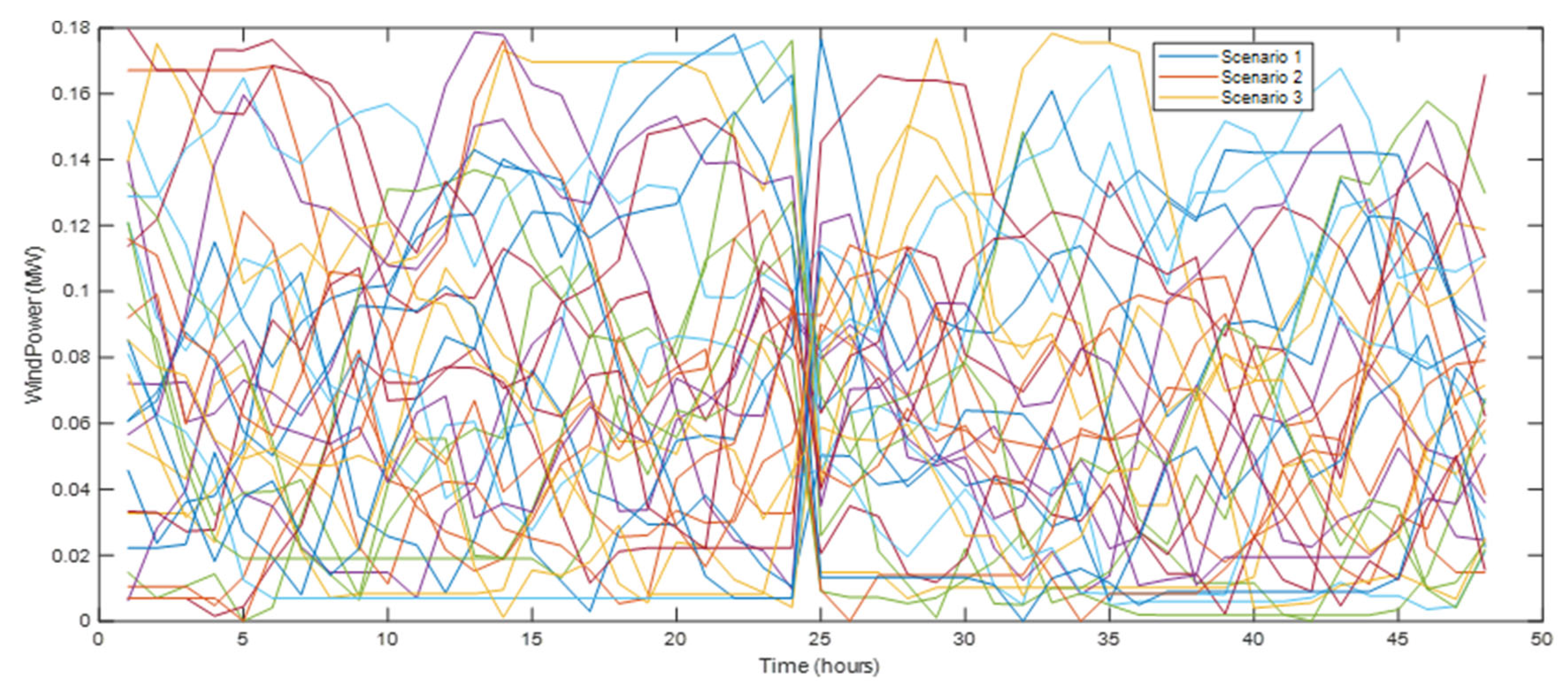
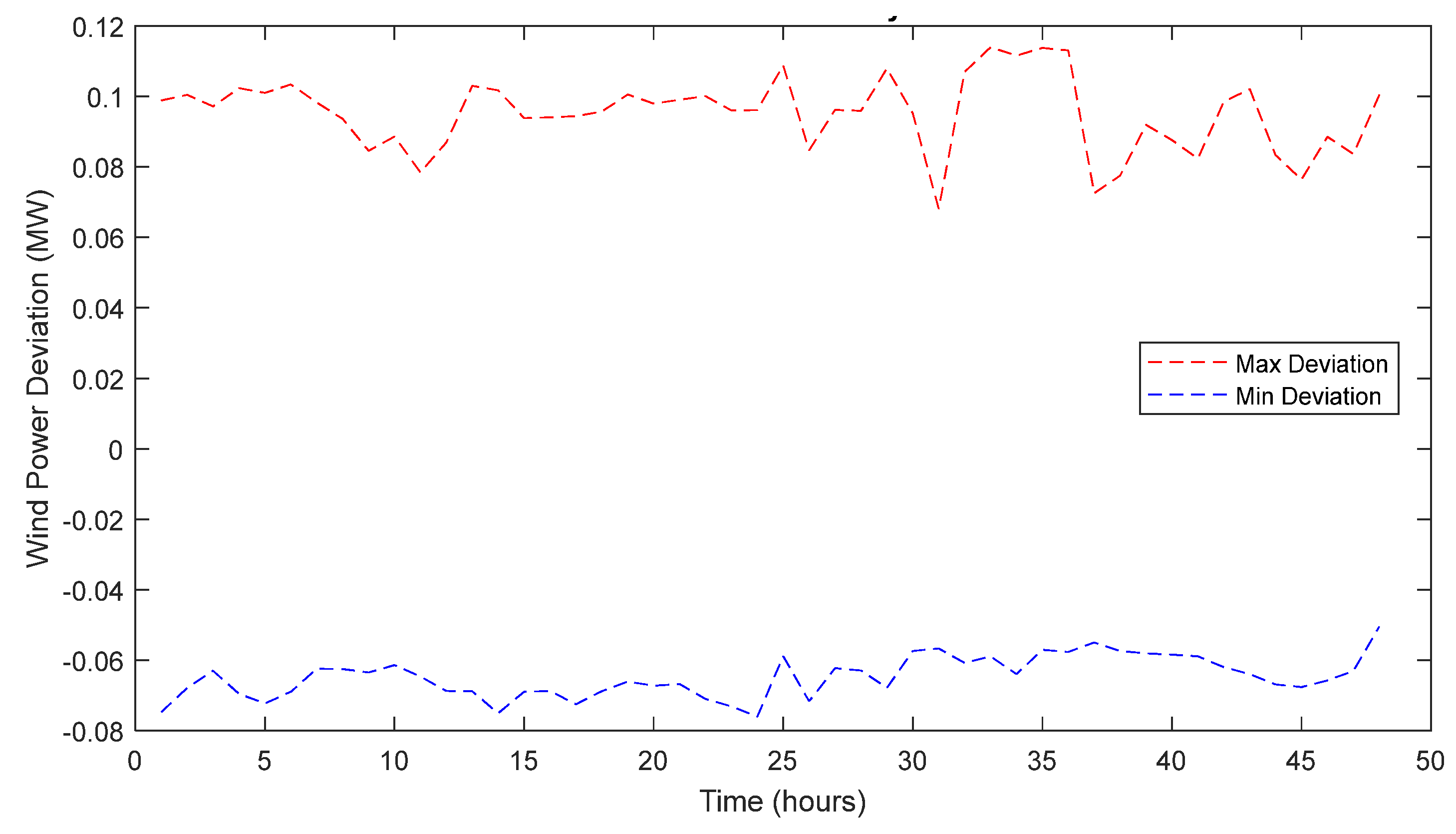
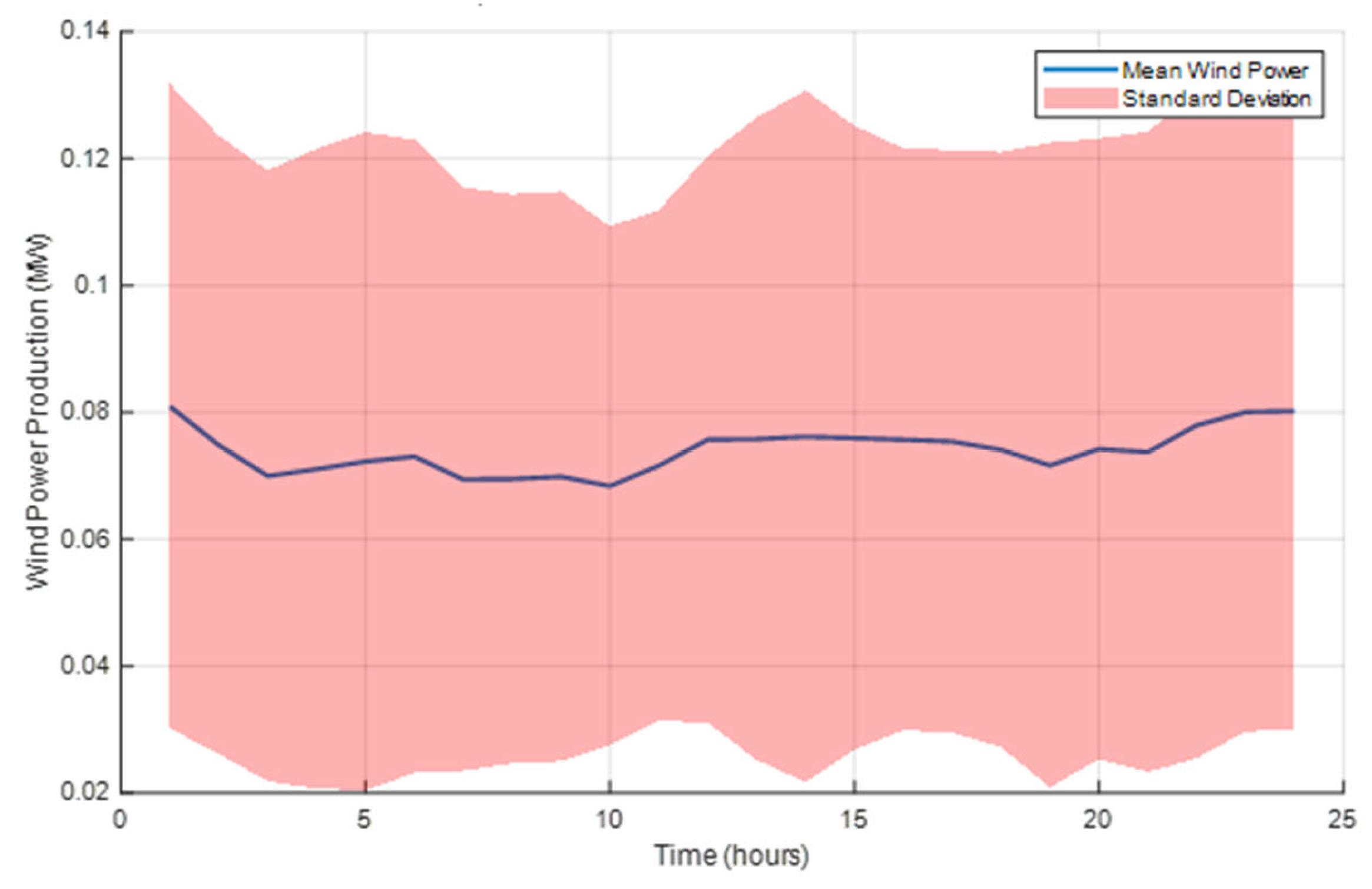
3.2. Wind Turbine
3.3. BESS
4. VPP Uncertainty Management
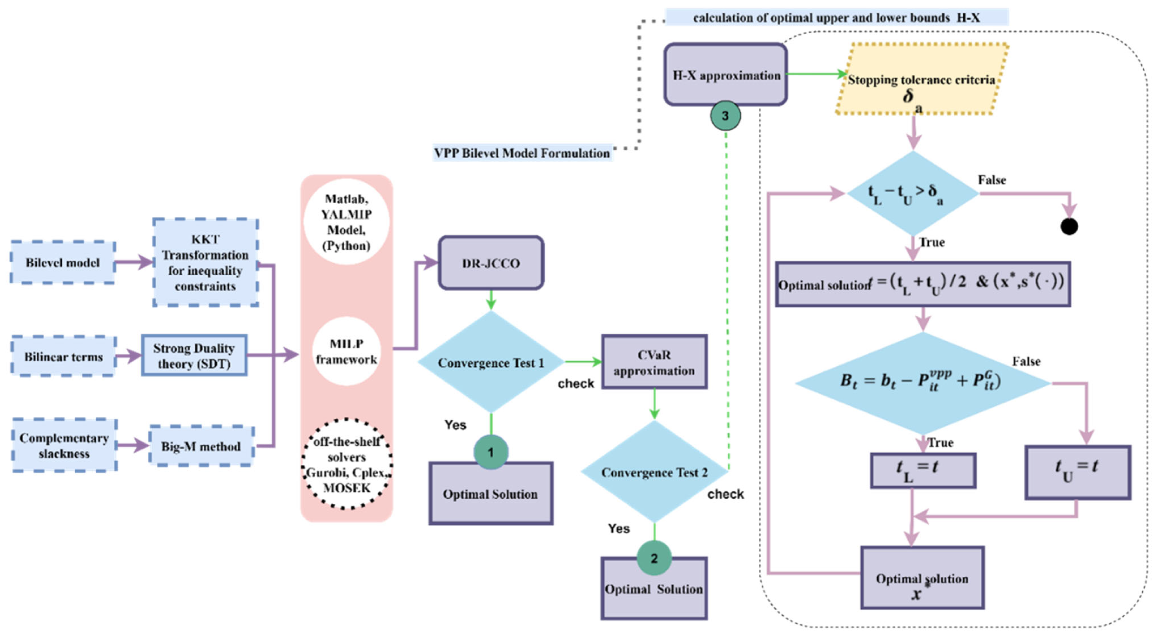
4.1. DR-JCCO-Approximating Algorithms
4.1.1. CVaR Application
4.1.2. H-X
4.1.3. General MPEC Formulation
5. Results
5.1. DR-JCCO-CVaR
5.2. DR-JCCO-H-X
6. Discussion
6.1. Conclusions
6.2. Future Work
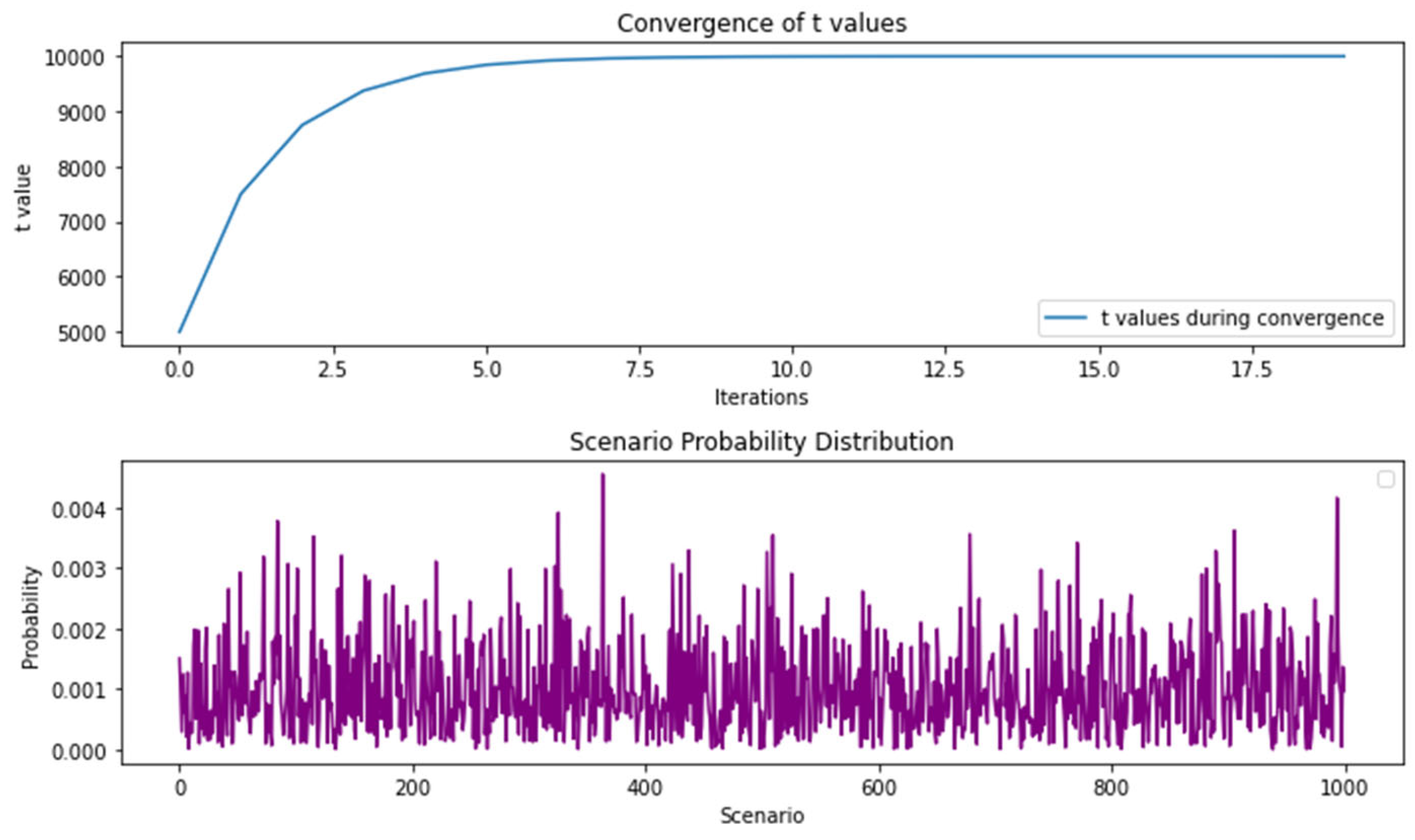
- Improvement of the H-X algorithm: Further research is needed to enhance the computation of the optimal t values within the H-X algorithm. This would improve its ability to regulate the charge–discharge cycles of the BESS, thereby facilitating more efficient long-term usage of the storage system and reducing degradation rates during operation.
- Dispatch of multiple VPPs: A potential area for future exploration involves the inclusion of multiple virtual power plants (VPPs). This would enable advanced analysis of coordinated scheduling and dispatch mechanisms across interconnected VPPs, a critical consideration for accurate and equitable settlement procedures in electricity markets.
- Advancement of EPEC models: While MPECs have received considerable attention, EPECs remain underexplored, specifically in the context of distribution networks. Future work should aim to bridge this gap.
Author Contributions
Funding
Data Availability Statement
Acknowledgments
Conflicts of Interest
Nomenclature
| Abbreviations | |
| WPP | Wind power plant |
| ISO | Independent system operator |
| TN | Transmission network |
| DN | Distribution network |
| MG | Microgrid |
| DG | Distributed generation |
| CHP | Combined heat and power |
| DGs | Diesel generators |
| DM | Day-ahead market |
| EPEC | Equilibrium problem with equilibrium constraints |
| KKT | Karush–Kuhn–Tucker |
| SP | Stochastic programming |
| RO | Robust optimization |
| JCC | Joint chance-constrained |
| Sets and indices | |
| i | Number of BESS index |
| Number of generator index | |
| 24 h | |
| CDF | Cumulative distribution function |
| System parameters | |
| Generators’ total power | |
| Utility function for battery storage system | |
| Difference between demand and renewable output | |
| Cost of storage energy per unit | |
| VPP generation | |
| VPP demand (electricity) | |
| Bid price | |
| Offer price | |
| TSO offering price | |
| VPP cost in DA | |
| Fuel cost | |
| Buying price for VPP | |
| Cost function for the generator | |
| Startup cost | |
| Minimum up time for unit g | |
| Minimum downtime for unit g | |
| Variables | |
| Aggregated VPP power in the electricity market | |
| Power demand at time t | |
| Discharged battery power | |
| Battery charging power | |
| Cleared power in DA in period t | |
| Cleared VPP demand in period t/BESS charged | |
| Optimal generator output in DA | |
| System market price | |
| Binary variable; if 1, the generator starts up | |
| Binary variable; if 0, the generator shuts down | |
Appendix A. Linearization of Continuous Variables
References
- Tiismus, H.; Maask, V.; Astapov, V.; Korõtko, T.; Rosin, A. State-of-the-Art Review of Emerging Trends in Renewable Energy Generation Technologies. IEEE Access 2025, 13, 10820–10843. [Google Scholar] [CrossRef]
- World Energy Transitions Outlook 2023. Available online: https://www.irena.org/Digital-Report/World-Energy-Transitions-Outlook-2023 (accessed on 28 February 2025).
- Onsomu, O.N.; Çetin, A.; Terciyanlı, E.; Yeşilata, B. Integration of Grid Scale Battery Energy Storage Systems and Application Scenarios. Eurasian J. Sci. Eng. Technol. 2024, 5, 76–86. [Google Scholar] [CrossRef]
- Beck, Y.; Ljubić, I.; Schmidt, M. A Brief Introduction to Robust Bilevel Optimization. arXiv 2022, arXiv:2211.16072. [Google Scholar] [CrossRef]
- Prat, E.; Chatzivasileiadis, S. Learning Active Constraints to Efficiently Solve Linear Bilevel Problems: Application to the Generator Strategic Bidding Problem. IEEE Trans. Power Syst. 2023, 38, 2376–2387. [Google Scholar] [CrossRef]
- Bracken, J.; McGill, J.T. Mathematical Programs with Optimization Problems in the Constraints. Oper. Res. 1973, 21, 37–44. [Google Scholar] [CrossRef]
- Birge, J.R.; Louveaux, F. Introduction to Stochastic Programming; Springer Series in Operations Research and Financial Engineering; Springer: New York, NY, USA, 2011; ISBN 978-1-4614-0236-7. [Google Scholar]
- Conejo, A.J.; Prieto, F.J. Mathematical programming and electricity markets. Top 2001, 9, 1–22. [Google Scholar] [CrossRef]
- Esfahani, M.M.; Hariri, A.; Mohammed, O.A. A Multiagent-Based Game-Theoretic and Optimization Approach for Market Operation of Multimicrogrid Systems. IEEE Trans. Ind. Inform. 2019, 15, 280–292. [Google Scholar] [CrossRef]
- Baillo, A.; Ventosa, M.; Rivier, M.; Ramos, A. Optimal Offering Strategies for Generation Companies Operating in Electricity Spot Markets. IEEE Trans. Power Syst. 2004, 19, 745–753. [Google Scholar] [CrossRef]
- Li, Y.; Li, H.; Wang, B.; Zhou, M.; Jin, M. Multi-objective unit commitment optimization with ultra-low emissions under stochastic and fuzzy uncertainties. Int. J. Mach. Learn. Cybern. 2021, 12, 1–15. [Google Scholar] [CrossRef]
- Jiang, N.; Xie, W. ALSO-X#: Better convex approximations for distributionally robust chance constrained programs. Math. Program. 2024. [Google Scholar] [CrossRef]
- Ben-Tal, A.; Nemirovski, A. Robust Convex Optimization. Math. Oper. Res. 1998, 23, 769–805. [Google Scholar] [CrossRef]
- Hanasusanto, G.A.; Roitch, V.; Kuhn, D.; Wiesemann, W. Ambiguous Joint Chance Constraints Under Mean and Dispersion Information. Oper. Res. 2017, 65, 751–767. [Google Scholar] [CrossRef]
- Guo, H.; Gong, D.; Zhang, L.; Wang, F.; Du, D. Hierarchical Game for Low-Carbon Energy and Transportation Systems Under Dynamic Hydrogen Pricing. IEEE Trans. Ind. Inform. 2023, 19, 2008–2018. [Google Scholar] [CrossRef]
- Zhao, W.; Diao, H.; Li, P.; Lv, X.; Lei, E.; Mao, Z.; Xue, W. Transactive Energy-Based Joint Optimization of Energy and Flexible Reserve for Integrated Electric-Heat Systems. IEEE Access 2021, 9, 14491–14503. [Google Scholar] [CrossRef]
- Cao, Y.; Wei, W.; Wang, J.; Mei, S.; Shafie-khah, M.; Catalao, J.P.S. Capacity Planning of Energy Hub in Multi-Carrier Energy Networks: A Data-Driven Robust Stochastic Programming Approach. IEEE Trans. Sustain. Energy 2020, 11, 3–14. [Google Scholar] [CrossRef]
- Chen, Y.; Guo, Q.; Sun, H.; Li, Z.; Wu, W.; Li, Z. A Distributionally Robust Optimization Model for Unit Commitment Based on Kullback–Leibler Divergence. IEEE Trans. Power Syst. 2018, 33, 5147–5160. [Google Scholar] [CrossRef]
- Zheng, W.; Huang, W.; Hill, D.J.; Hou, Y. An Adaptive Distributionally Robust Model for Three-Phase Distribution Network Reconfiguration. IEEE Trans. Smart Grid 2021, 12, 1224–1237. [Google Scholar] [CrossRef]
- Yan, M.; Shahidehpour, M.; Paaso, A.; Zhang, L.; Alabdulwahab, A.; Abusorrah, A. Distribution Network-Constrained Optimization of Peer-to-Peer Transactive Energy Trading Among Multi-Microgrids. IEEE Trans. Smart Grid 2021, 12, 1033–1047. [Google Scholar] [CrossRef]
- Wang, Z.; Chen, B.; Wang, J.; Kim, J. Decentralized Energy Management System for Networked Microgrids in Grid-Connected and Islanded Modes. IEEE Trans. Smart Grid 2016, 7, 1097–1105. [Google Scholar] [CrossRef]
- Saber, H.; Ehsan, M.; Moeini-Aghtaie, M.; Ranjbar, H.; Lehtonen, M. A User-Friendly Transactive Coordination Model for Residential Prosumers Considering Voltage Unbalance in Distribution Networks. IEEE Trans. Ind. Inform. 2022, 18, 5748–5759. [Google Scholar] [CrossRef]
- Wang, Z.; Chen, B.; Wang, J.; Begovic, M.M.; Chen, C. Coordinated Energy Management of Networked Microgrids in Distribution Systems. IEEE Trans. Smart Grid 2015, 6, 45–53. [Google Scholar] [CrossRef]
- Liu, Z.; Wang, L.; Ma, L. A Transactive Energy Framework for Coordinated Energy Management of Networked Microgrids with Distributionally Robust Optimization. IEEE Trans. Power Syst. 2020, 35, 395–404. [Google Scholar] [CrossRef]
- Sheikhahmadi, P.; Bahramara, S.; Mazza, A.; Chicco, G.; Catalão, J.P.S. Bi-level optimization model for the coordination between transmission and distribution systems interacting with local energy markets. Int. J. Electr. Power Energy Syst. 2021, 124, 106392. [Google Scholar] [CrossRef]
- Mahboubi-Moghaddam, E.; Nayeripour, M.; Aghaei, J.; Khodaei, A.; Waffenschmidt, E. Interactive Robust Model for Energy Service Providers Integrating Demand Response Programs in Wholesale Markets. IEEE Trans. Smart Grid 2018, 9, 2681–2690. [Google Scholar] [CrossRef]
- Daneshvar, M.; Mohammadi-Ivatloo, B.; Zare, K.; Asadi, S.; Anvari-Moghaddam, A. A Novel Operational Model for Interconnected Microgrids Participation in Transactive Energy Market: A Hybrid IGDT/Stochastic Approach. IEEE Trans. Ind. Inform. 2021, 17, 4025–4035. [Google Scholar] [CrossRef]
- Daneshvar, M.; Mohammadi-Ivatloo, B.; Zare, K.; Asadi, S. Two-Stage Robust Stochastic Model Scheduling for Transactive Energy Based Renewable Microgrids. IEEE Trans. Ind. Inform. 2020, 16, 6857–6867. [Google Scholar] [CrossRef]
- Zheng, X.; Qu, K.; Lv, J.; Li, Z.; Zeng, B. Addressing the Conditional and Correlated Wind Power Forecast Errors in Unit Commitment by Distributionally Robust Optimization. IEEE Trans. Sustain. Energy 2021, 12, 944–954. [Google Scholar] [CrossRef]
- Chen, Y.; Wei, W.; Liu, F.; Mei, S. Distributionally robust hydro-thermal-wind economic dispatch. Appl. Energy 2016, 173, 511–519. [Google Scholar] [CrossRef]
- Zhong, J.; Li, Y.; Wu, Y.; Cao, Y.; Li, Z.; Peng, Y.; Qiao, X.; Xu, Y.; Yu, Q.; Yang, X.; et al. Optimal Operation of Energy Hub: An Integrated Model Combined Distributionally Robust Optimization Method with Stackelberg Game. IEEE Trans. Sustain. Energy 2023, 14, 1835–1848. [Google Scholar] [CrossRef]
- Bagchi, A.; Xu, Y. Distributionally Robust Chance-Constrained Bidding Strategy for Distribution System Aggregator in Day-Ahead Markets. In Proceedings of the 2018 IEEE International Conference on Communications, Control, and Computing Technologies for Smart Grids (SmartGridComm), Aalborg, Denmark, 29–31 October 2018; IEEE: Aalborg, Denmark, 2018; pp. 1–6. [Google Scholar]
- Wang, R.; Wang, P.; Xiao, G. A robust optimization approach for energy generation scheduling in microgrids. Energy Convers. Manag. 2015, 106, 597–607. [Google Scholar] [CrossRef]
- Ben-Tal, A.; Den Hertog, D.; De Waegenaere, A.; Melenberg, B.; Rennen, G. Robust Solutions of Optimization Problems Affected by Uncertain Probabilities. Manag. Sci. 2013, 59, 341–357. [Google Scholar] [CrossRef]
- Jiang, R.; Guan, Y. Data-driven chance constrained stochastic program. Math. Program. 2016, 158, 291–327. [Google Scholar] [CrossRef]
- Ahmed, S.; Luedtke, J.; Song, Y.; Xie, W. Nonanticipative duality, relaxations, and formulations for chance-constrained stochastic programs. Math. Program. 2017, 162, 51–81. [Google Scholar] [CrossRef]
- Wu, Y.; Liu, Z.; Liu, J.; Xiao, H.; Liu, R.; Zhang, L. Optimal battery capacity of grid-connected PV-battery systems considering battery degradation. Renew. Energy 2022, 181, 10–23. [Google Scholar] [CrossRef]


| Ref # | Problem Formulation | Modeling Levels | Uncertainty | Solution Algorithms | |
|---|---|---|---|---|---|
| Upper Level | Lower Level | ||||
| [9] | Bilevel | DN | MG | RO | ADMM |
| [15] | Bilevel | Energy hub | EVs | SP | — |
| [16] | Bilevel | Energy hub | Users | Two-stage RO | C&CG |
| [17] | Energy hub | Energy hub | Users and EVs | KL-based DRO | Crafted C&CG (linearization of USP) |
| [18] | Single level | — | — | KL-based DRO | Outer approximation |
| [19] | Single level | — | — | KL-based DRO | Benders decomposition |
| [20] | Single level | — | — | KL-based DRO | C&CG |
| [21] | Bilevel | DN | MG | — | Stackelberg game |
| [22] | Bilevel | DN | MG | RO | ADMM |
| [23] | Bilevel | DN | MG | — | Noncooperative game |
| [24] | Bilevel | DN | MG | — | KKT |
| [25] | Bilevel | DN | MG | DRO | KKT |
| [26] | Bilevel | TN | DN | IGDT | KKT |
| [27] | Bilevel | TN | DN | RO | Iterative method (two steps) |
| [28] | Single level | TN | MG | IGDT-SP | — |
| [29] | Bilevel | TN | MG | RO-SP | Dantzig–Wolfe |
| [30,31] | Single level | — | — | Moment-based DRO | Delayed constraint generation |
| Proposed | Bilevel VPP | Day-ahead market | VPP owners | DR-JCCO | CVaR&H-X |
| Optimization Approach | Performance Metrics | ||||||
|---|---|---|---|---|---|---|---|
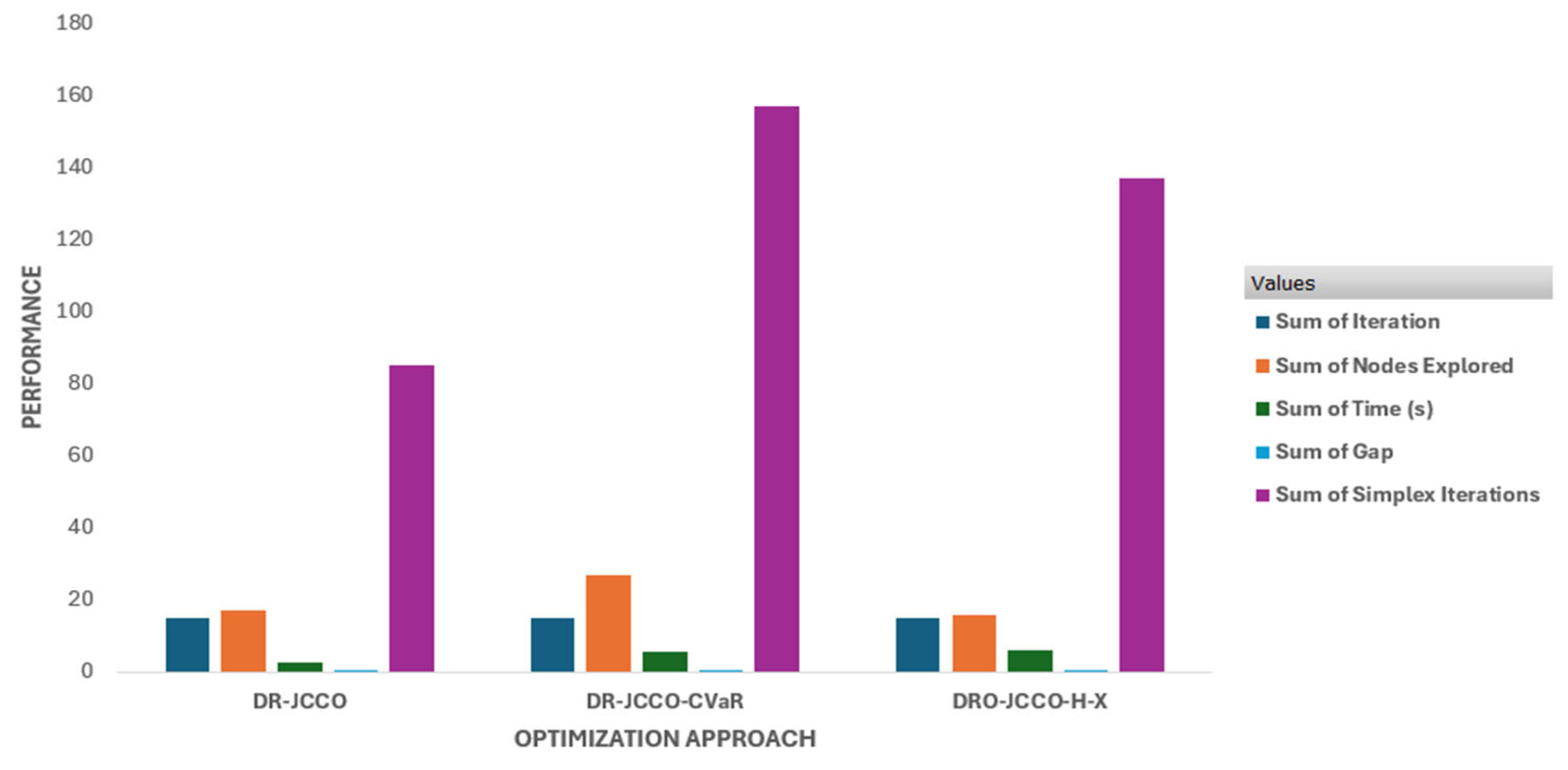
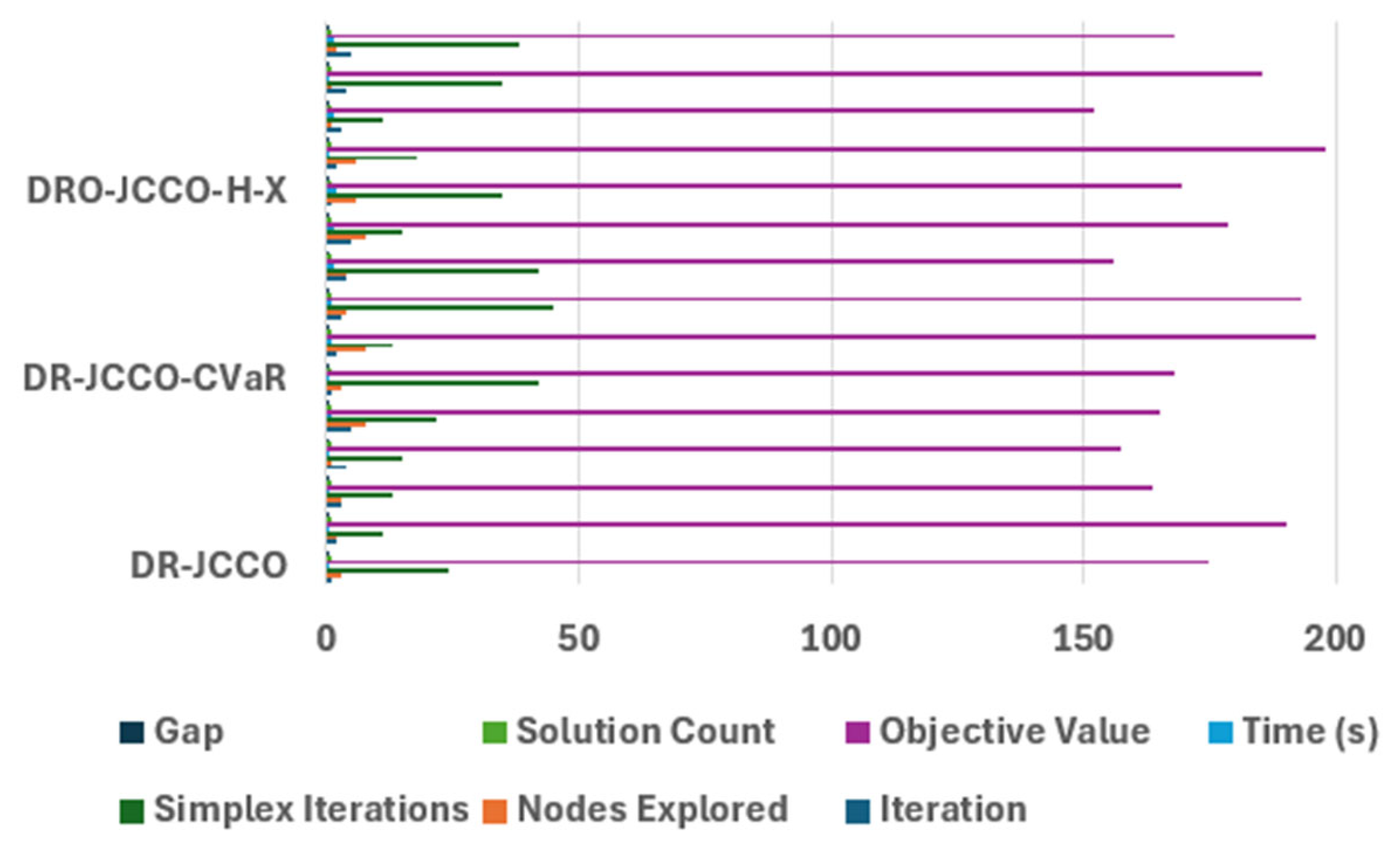
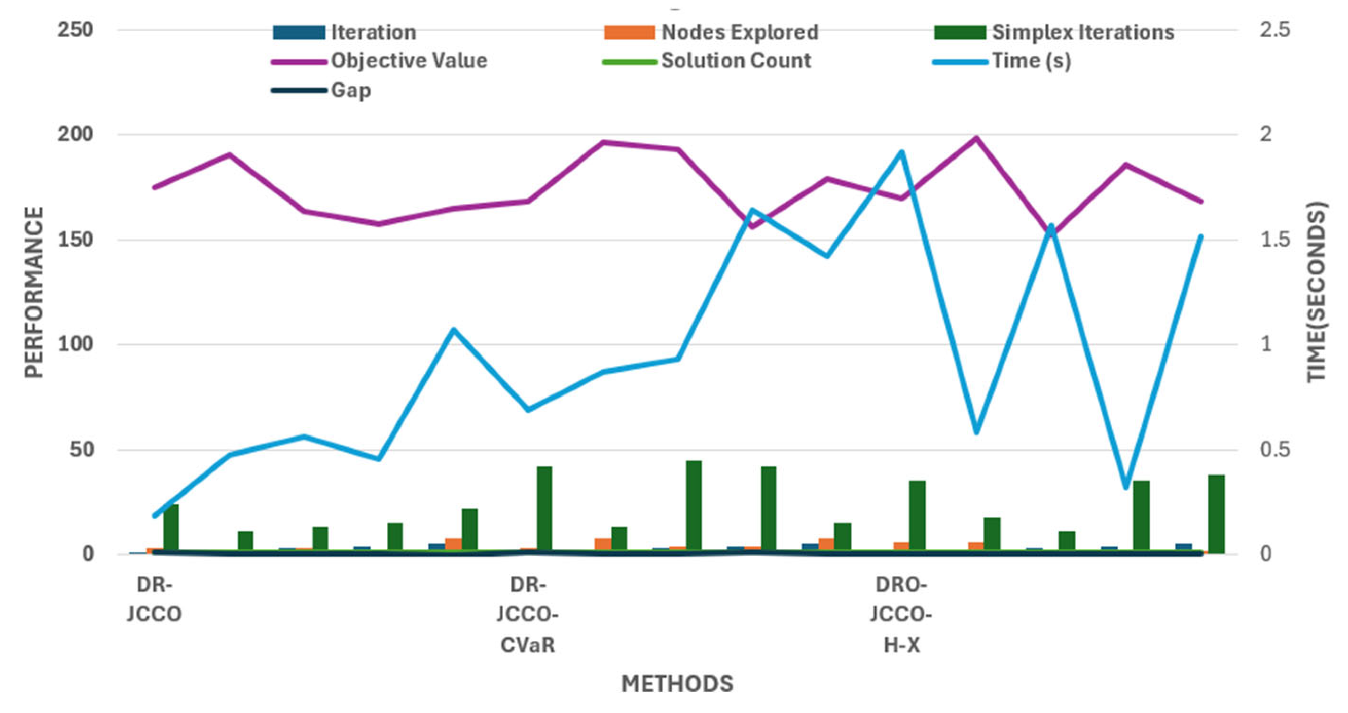
| Sum of Iteration | Summing Nodes Explored | Sum of Time (s) | Sum of Gap | Summing Simplex Iterations | Conservativeness of Solutions | Tractability Level | |
| DR-JCCO | 15 | 17 | 2.73848223 | 0.022970004 | 85 | High | Low |
| DR-JCCO-CVaR | 15 | 27 | 5.54975679 | 0.028598226 | 157 | Moderate | High |
| DR-JCCO-H-X | 15 | 16 | 5.90154595 | 0.021566176 | 137 | Low | Best |
Disclaimer/Publisher’s Note: The statements, opinions and data contained in all publications are solely those of the individual author(s) and contributor(s) and not of MDPI and/or the editor(s). MDPI and/or the editor(s) disclaim responsibility for any injury to people or property resulting from any ideas, methods, instructions or products referred to in the content. |
© 2025 by the authors. Licensee MDPI, Basel, Switzerland. This article is an open access article distributed under the terms and conditions of the Creative Commons Attribution (CC BY) license (https://creativecommons.org/licenses/by/4.0/).
Share and Cite
Onsomu, O.N.; Terciyanlı, E.; Yeşilata, B. Optimal Dispatch of a Virtual Power Plant Considering Distributed Energy Resources Under Uncertainty. Energies 2025, 18, 4012. https://doi.org/10.3390/en18154012
Onsomu ON, Terciyanlı E, Yeşilata B. Optimal Dispatch of a Virtual Power Plant Considering Distributed Energy Resources Under Uncertainty. Energies. 2025; 18(15):4012. https://doi.org/10.3390/en18154012
Chicago/Turabian StyleOnsomu, Obed N., Erman Terciyanlı, and Bülent Yeşilata. 2025. "Optimal Dispatch of a Virtual Power Plant Considering Distributed Energy Resources Under Uncertainty" Energies 18, no. 15: 4012. https://doi.org/10.3390/en18154012
APA StyleOnsomu, O. N., Terciyanlı, E., & Yeşilata, B. (2025). Optimal Dispatch of a Virtual Power Plant Considering Distributed Energy Resources Under Uncertainty. Energies, 18(15), 4012. https://doi.org/10.3390/en18154012