Abstract
The large-scale integration of new energy is an inevitable trend to achieve the low-carbon transformation of power systems. However, the strong randomness of wind power, photovoltaic power, and loads poses severe challenges to the safe and stable operation of systems. Existing studies demonstrate insufficient integration and handling of source-load bilateral uncertainties in wind–solar–fossil fuel storage complementary systems, resulting in difficulties in balancing economy and low-carbon performance in their energy storage configuration. To address this insufficiency, this study proposes an optimal energy storage configuration method considering source-load uncertainties. Firstly, a deterministic bi-level model is constructed: the upper level aims to minimize the comprehensive cost of the system to determine the energy storage capacity and power, and the lower level aims to minimize the system operation cost to solve the optimal scheduling scheme. Then, wind and solar output, as well as loads, are treated as fuzzy variables based on fuzzy chance constraints, and uncertainty constraints are transformed using clear equivalence class processing to establish a bi-level optimization model that considers uncertainties. A differential evolution algorithm and CPLEX are used for solving the upper and lower levels, respectively. Simulation verification in a certain region shows that the proposed method reduces comprehensive cost by 8.9%, operation cost by 10.3%, the curtailment rate of wind and solar energy by 8.92%, and carbon emissions by 3.51%, which significantly improves the economy and low-carbon performance of the system and provides a reference for the future planning and operation of energy systems.
1. Introduction
With the proposal of the “carbon emission reduction” initiative, building a new-type power system with new energy as the main body has become one of the core tasks in the development of the energy industry [1]. Renewable energies, such as solar energy and wind energy, play an important role in new-type power systems [2]. Compared with traditional fossil fuel power generation, new energy power generation produces almost no greenhouse gases, such as carbon dioxide, during operation, which can effectively reduce carbon emissions and provide a feasible path for achieving low-carbon power supply and alleviating the pressure of global warming [3]. However, the large-scale integration of new energy has brought significant challenges to the power grid. Reference [4] points out that the uncertainty of new energy output increases the regulation burden of power systems. When new energy output exceeds a system’s regulation range, power curtailment must be carried out to ensure the real-time balance between power generation and consumption, leading to phenomena such as the curtailment of wind and solar power and limited absorption [5]. In addition, load demand is affected by various factors such as seasonal climate, social habits, residents’ economic level, and electricity price policies, showing complex and variable fluctuation characteristics on different time scales. The interweaving of uncertainties on the source side and load side further exacerbates the complexity of system operation [6].
Against this background, energy storage has become a key factor in realizing the optimal allocation of power system resources and promoting the efficient utilization of renewable energy. Combining energy storage with a wind–solar–fossil fuel complementary energy system can flexibly adjust the system’s operation mode, cope with load-side volatility and the uncertainty and uncontrollability of new energy, improve the quality of the user power supply, and reduce the impact of new energy integration on the power grid, thus ensuring the supply–demand balance of the power system and improving system reliability [7].
Reviewing the existing literature, many scholars have carried out extensive research on source-load uncertainty and energy storage configuration optimization in multi-energy systems, and they have achieved a series of phased results. Wang proposed a multi-time scale optimization method considering source-load uncertainty. Based on fuzzy chance-constrained programming theory, using mathematical modeling and multi-scenario technology, source-load uncertainty is incorporated into day-ahead and real-time scheduling models. The results show that this optimization strategy can effectively alleviate the impact of source-load uncertainty while maintaining system economy [8]. Yao used Markov chain Monte Carlo simulation to generate a large number of source-load scenarios, proposed a discrete state optimization selection method, and reduced scenarios using fast-forward elimination technology to obtain typical time series curves characterizing source-load uncertainty [9]. An adopted the DPMM to construct uncertainty fuzzy sets of photovoltaic power generation and load demand, aiming to reduce the negative impact of uncertain factors, and used the column-and-constraint generation algorithm to solve the constructed optimization model [10]. Xing proposed a bi-level scheduling method for energy storage considering power source and load uncertainty, handling the uncertainty of wind power, photovoltaic power, and load through fuzzy parameters [11].
With the widespread application of renewable energy, the issue of energy storage configuration has also become a research hotspot. The randomness, volatility, and intermittency of renewable energy have brought great challenges to the operational stability of power systems. Liu reviewed the latest progress in the applications, modeling methods, and optimal configuration strategies of energy storage in multiple fields such as power generation, grid management, and user-side factors [12]. Huang constructed a bi-level optimization model for energy storage capacity configuration and operation of the wind–solar storage microgrid system, using an improved gray wolf optimization algorithm to adjust photovoltaic, wind power, and load fluctuations, optimizing energy storage economy and efficiency and improving the overall system performance [13]. Lei constructed an optimal configuration model for hybrid energy storage system capacity, using variational mode decomposition (VMD) to realize energy storage allocation in a wind–solar complementary system, showing that this method is more economical than traditional allocation strategies [14]. Wu proposed an energy storage configuration optimization framework based on the NSGA-II and TOPSIS algorithms, determining the optimal capacity and continuous energy storage duration using calculation and analysis [15]. Tian proposed a full-life-cycle energy storage configuration optimization method for new energy power stations based on the improved gray wolf optimization algorithm (IGWOA), and the model has a significant effect in reducing the curtailment of wind and solar power and improving the net income of energy storage [16]. Ye introduced the gravitational search algorithm to optimize the energy storage capacity of a wind–solar storage combined network, improving voltage stability and reducing load fluctuations [17]. Ma used a deep learning-based Wasserstein GAN model to generate wind–solar output scenarios, and then constructed a hybrid system capacity configuration optimization model and solve it using the sparrow search algorithm, and the results verified the effectiveness and practicability of the model [18]. Zheng proposed an energy storage optimization strategy for photovoltaic-dominated power grids, considering source-load imbalance clustering, aiming to minimize voltage deviation, power loss, and operation cost, and used a hybrid particle swarm optimization method to determine the optimal installation location and capacity of energy storage [19]. Huang improved the simulated annealing algorithm, aiming to minimize the probability of power supply loss, cost, and energy allocation reliability, and showed better performance in solving the optimal configuration of a wind–solar storage battery system [20]. Zhao examined the role of hydrogen fuel cell vehicles (HFCVs) in integrating green hydrogen into energy and transport systems, the challenges faced (including green hydrogen production, techno-economic, and policy barriers), and provided a roadmap to overcome these obstacles for developing the hydrogen economy [21].
However, due to immature technologies, some problems still exist. Dong proposed a multi-objective configuration optimization model for the coordination of renewable energy output uncertainty and user-side demand response, but the model has insufficient consideration of the economy of energy storage configuration. Due to the failure to fully optimize the full-life-cycle cost, the energy storage investment is too high, restricting its application and promotion [22]. Wang constructed a hierarchical optimization framework based on electrical and thermal load characteristics, and verified the operation strategy and configuration scheme of hybrid electrical-thermal energy storage through multiple scenarios. However, the system design has integrity defects. Due to the failure to incorporate equipment cost parameters and full-cycle comprehensive economic analysis, the economic reference value of the optimization results is limited [23]. Li proposed a coupling scheme of compressed-air energy storage and coal-fired power plants for the coupled application of traditional power sources and energy storage. However, due to the lack of a heat storage capacity evaluation, key reliability constraints are omitted in the model construction, which may lead to insufficient system stability in actual operation [24]. Xu carried out research on energy storage configuration in high-penetration photovoltaic scenarios, established an adaptability optimization model, and analyzed the impact of photovoltaic power generation on energy storage capacity. However, the research scenario is limited to a single weather condition, and the temporal and spatial differences are not considered, resulting in the model lacking universal system data support and being difficult to adapt to diverse engineering scenarios [25]. Moreover, most existing studies consider source-load output uncertainty when discussing system scheduling schemes, while there are few studies that incorporate source-load uncertainty into energy storage configuration research. The uncertainty of source-load output affects the configuration capacity of energy storage, which in turn relates to the economy and stability of system investment and operation. Existing achievements still have significant limitations in the optimization of energy storage configuration in wind–solar–fossil fuel complementary systems: on the one hand, most studies simplify the handling of source-load uncertainty, either focusing only on the single-fluctuation characteristics of new-energy output or failing to effectively integrate the dynamic changes in load demand, leading to the neglect of the coupling effect of bilateral uncertainties. On the other hand, in model construction, the transformation methods for uncertain constraints are insufficient, making it difficult to accurately quantify their impacts on energy storage capacity configuration, resulting in configuration results often being conservative or radical, and failing to balance economy and reliability; in addition, the linkage mechanism between energy storage configuration and system scheduling in existing studies is insufficient, which easily leads to problems such as a high curtailment rate of wind and solar power, increased operation cost, or unsatisfactory carbon emission control in actual operation, which cannot meet the multiple requirements of the new-type power system for economy, environmental protection, and stability in the context of low-carbon transformation. Therefore, it is urgent to construct an energy storage configuration optimization model integrating source-load uncertainty to improve the accuracy and practicability of configuration schemes.
In the field of energy system optimization, fuzzy chance constraints and the bi-level DE + CPLEX hybrid solution method have become important technical means to deal with uncertainty and complex hierarchical problems. In previous studies, fuzzy chance constraints have been widely used in the optimization of power systems with high proportions of new energy, integrated energy systems, and microgrids. Ma applied it to the configuration of wind–solar storage complementary systems, achieving the balance between system safety and economy by incorporating fuzzy uncertain variables such as wind power, photovoltaic output, and load and setting reasonable confidence levels [26]. Kevin solves the optimal economic dispatch problem for multiple islands, taking into account realistic offshore renewable energy technologies to better address the siting of isolated microgrids, microgrid design and storage sizing [27]. In contrast, the bi-level DE + CPLEX hybrid solution method, as an efficient solution framework for hierarchical optimization, is mainly applied to complex problems that require collaborative optimization of planning and operation. Li proposed a bi-level coordinated optimization strategy for the external response of multi-energy complementary micro-energy networks based on shared energy storage stations. This study divides a multi-energy complementary micro-energy network system into upper and lower layers, and calls CPLEX to solve the model. The simulation results show that this strategy can reduce the operation cost of micro-energy network operators by 6.3% [28]. Tiwari proposes a rapid line protection scheme based on Pole Differential Current (PDC) for LCC-HVDC transmission systems. Simulation analysis demonstrates its capability to reliably detect fault poles within 5.1 ms during bipolar operation and 15.6 ms during monopolar operation while exhibiting strong noise immunity [29]. Gao adopted this method in multi-energy collaborative scheduling of microgrids, improving the solution efficiency of complex systems through hierarchical optimization [30].
This study proposes a bi-level optimization configuration method for energy storage in wind–solar–fossil fuel complementary energy systems considering source-load uncertainty and constructs a wind–solar–fossil fuel storage configuration optimization model considering source-load uncertainty. Based on fuzzy chance constraints, wind power output, photovoltaic output, and load are regarded as fuzzy variables to handle the uncertainty on both source and load sides, and the uncertain constraints are transformed into deterministic constraints through clear equivalence class processing. The upper layer solves the optimal energy storage configuration to minimize the comprehensive system cost, and the lower layer solves the optimal scheduling scheme to minimize the system operation cost. The differential evolution algorithm and CPLEX are used to solve the model. Compared to previous studies, the innovations and improvements of this paper are mainly reflected in two aspects: First, although some studies adopt the bi-level DE + CPLEX hybrid solution method, most of them regard energy storage configuration and system scheduling as independent links, which are only related through simple parameter transmission, easily leading to the disconnection between configuration results and actual operation needs. In this study, an “upper layer for energy storage capacity and power configuration-lower layer for system operation scheduling” deeply coupled bi-level model is constructed. The upper and lower layers are solved by the differential evolution algorithm and CPLEX, respectively, enabling the configuration scheme and operation strategy to form a dynamic response mechanism, avoiding economic losses or reliability risks caused by traditional separate optimization. Second, aiming at the limitation that previous studies focus on a single economic objective, this paper synchronously incorporates multi-dimensional indicators such as comprehensive cost, operation cost, curtailment rate of wind and solar power, and carbon emissions into the bi-level optimization framework. Through the quantitative control of uncertainty by fuzzy chance constraints and the efficient solution of the hybrid method, the collaborative optimization of economy, environmental protection, and system stability is realized, which is more in line with the actual needs of the new-type power system in low-carbon transformation and fills the gap around multi-objective balance in existing studies.
2. Model Construction
2.1. Deterministic Energy Storage Capacity Allocation Modeling
In this paper, a two-layer optimization framework is used, where the upper layer decides the storage allocation capacity, with the objective of minimizing the total system cost, and the lower layer receives the storage allocation results and solves the optimal operation strategy, with the objective of minimizing the system operation cost. The two-layer model interaction structure is shown in Figure 1.
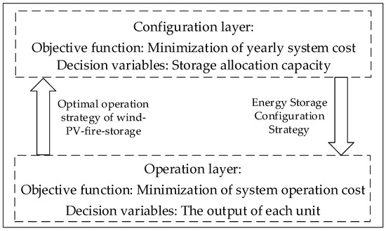
Figure 1.
Two-layer optimization model interaction structure.
2.1.1. Configuration Layer
- 1.
- Objective function
The goal function of the energy storage capacity configuration layer is to minimize the overall yearly system cost, which includes the annualized energy storage investment cost and the system’s annual operating cost.
In the formula, is the energy storage system’s annualized investment cost and is the system’s annual operating cost.
where is the configured capacity of energy storage, is the unit capacity construction cost of energy storage, is the unit capacity maintenance cost of energy storage, is the configured power of energy storage, is the unit power construction cost of energy storage, is the discount rate, and is the lifetime of energy storage.
- 2.
- Constraints
Wind and solar abandonment rates decrease with increasing energy storage configuration scale, but investment costs rise with its expansion. There is an upper limit to the configuration power and capacity of energy storage from an economic perspective.
In the formula, is the energy storage configuration capacity limit value and is the energy storage configuration power limit value.
2.1.2. Operation Layer
The operation layer takes the minimization of system operation cost as the objective function and takes power balance constraints, standby capacity constraints, wind and light output constraints, and energy storage charging and discharging constraints as the dominant constraints, and decides the output of each unit.
- 1.
- Objective function
In the formula, is the cost of the coal consumption of thermal power units, is the starting and stopping cost of the thermal power units, is the cost of carbon emissions, and is the cost of abandoned wind and PV, which refers to the opportunity cost of curtailed renewable energy that could not be utilized by the power grid. The capital composition during the operation of the system is shown in Figure 2:
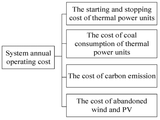
Figure 2.
Capital flow model during system operation.
The coal-fired power unit coal consumption cost is determined by the coal price over coal consumption; the start–stop cost is determined by the number of start–stops and the cost of a single start–stop; the CO2 cost is determined by the power of the coal-fired power units, the CO2 emission coefficient, and the carbon price; and the cost of the wind and PV energy abandonment is determined by the amount of electricity abandoned and the cost of the wind and PV energy abandonment penalties.
In the formula, is the power output of thermal power units at the time, are the coal consumption coefficient of thermal power units, and is the coal price. are the number of switching times of thermal power units, is the single switching cost of thermal power units, is the carbon emission coefficient, and is the carbon trading price. represent the actual output of PV units and WTGs at the time, represent the predicted output of PV units and WTGs at the time, and represent the unit cost of wind abandonment and the unit cost of light abandonment.
- 2.
- Constraints
The power balance constraints for each unit and load in the system are as follows:
In the formula, represents the power of thermal power units at the time, represent the power of wind power units and photovoltaic units at the time, represent the charging and discharging power of the energy storage system at the time, and represents the load at the time.
There are maximum and minimum output constraints for thermal power units in the operation process, as shown in Equation (7).
In the formula, symbolize the thermal power units’ lowest and maximum outputs, respectively.
The thermal power unit is limited by its climbing ability to change the rate of load rise and fall of the unit, as shown in Equation (8).
In the formula, indicates the downward climbing rate of thermal power unit and indicates the upward climbing rate of thermal power unit.
The output of wind PV is constrained by the upper limit of its installed capacity, as shown in Equation (9).
In the formula, denote the maximum output power of the wind units and PV units.
The following is an expression for the energy storage system’s charging and discharging constraint.
In the formula, show the energy storage equipment’s charging and discharging power at time t, respectively; indicates the charging and discharging coefficient of the energy storage equipment at time t, which takes the value of 0 or 1; indicates the residual charge state of the energy storage equipment at time t; , indicate the charging and discharging efficiency of the energy storage equipment; indicates the remaining charge state of the energy storage device at time t; and indicate the maximum charge state and minimum charge state of the energy storage device, respectively.
2.2. Energy Storage Capacity Allocation Model, Taking into Account the Uncertainty of Source and Load Outputs
There are many prediction methods and techniques for the power prediction of uncertain power sources and loads such as wind power, but due to the influence of natural conditions and other unknown external factors, there are still errors between the predicted results and the actual power source and load power. When the wind power large-scale connected grid and load size is large, these prediction errors cannot be ignored. In the power system day-ahead scheduling model, wind power output and load power are uncertain variables. Therefore, the actual values of wind and load considering the prediction errors can be described as
In the formula, , respectively, represent the actual power of WTGs and PVGs at the time; , respectively, represent the predicted power of WTGs and PVGs at the time; respectively, represent the deviation of the predicted power of WTGs and PVGs at the time; represents the actual load at the time; represents the predicted load at the time; and represents the deviation of the load prediction at the time.
When the prediction error is taken into account, the deterministic energy storage capacity allocation model is no longer applicable, and the new power balance constraint is obtained by coupling Equations (6) and (11) as follows:
In this paper, fuzzy treatment of chance constraints is used. Fuzzy chance constraints are the theories that optimize the objective function under the condition that the probability under satisfying the uncertainty constraint tuning is not less than a given confidence level. The opportunity constraint model is
In the formula, is the objective function containing random variables, is the probability that the event in curly brackets holds, and is the confidence level.
Therefore, the source-load uncertainty-accounting energy storage allocation model can be written as follows:
The general method to solve the fuzzy-chance-constrained planning problem is to utilize some kind of linear relationship or to separate the fuzzy variables from the deterministic variables and transform the fuzzy variables into clear equivalence classes.
In this paper, the trapezoidal subordination function is used to describe the uncertainty of the photovoltaic output and load:
where is the trapezoidal affiliation function of , is the fuzzy parameter in the system, is the predicted value, is the affiliation parameter of scenery and load, and is the scale parameter, which is generally determined by the historical data of the fuzzy parameter.
The trapezoidal fuzzy parameters are shown in Figure 3:
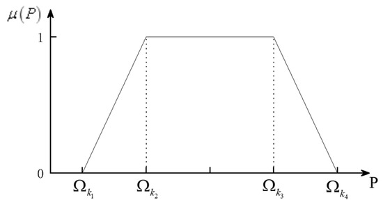
Figure 3.
Trapezoidal fuzzy parameters.
The constraint function has the following form:
where is a function containing only decision variables and is the trapezoidal fuzzy parameter, . Where , is the trapezoidal affiliation parameter.
Define the following two functions:
Specifically, when , , , and when , , . Considering the safety of the system, the confidence level should not be too low, so take the clear equivalence class of opportunity constraint as
The power balance clear equivalence class is
In the formula, is the affiliation parameter of load in the system, is the affiliation parameter of PV in the system, and is the affiliation parameter of PV in the system.
Based on the power balance clear equivalence class, the differential evolutionary algorithm and CPLEX commercial solver are adopted to solve the problem.
2.3. Model Solution
In the two-layer optimization model, the upper optimization model is the optimization of the capacity and power allocation of the energy storage equipment, the optimization of the energy storage configuration is based on the objective of minimizing the total cost of the upper system, and the result is the initial value of the lower operation; the decision variables are the capacity and power of the storage equipment, the differential evolution algorithm has better applicability and robustness in solving the optimization problem compared to traditional genetic algorithms and particle swarm algorithms, and the adaptive differential evolution algorithm improves the global search capability by introducing adaptive parameter factors and multi-strategy variations. The adaptive differential evolutionary algorithm improves the global search capability of the algorithm through the introduction of adaptive parameter factors and multi-strategy variants, and the chromosome in the adaptive differential evolutionary algorithm can encode the decision variables in a simpler way; therefore, this paper adopts the adaptive differential evolutionary algorithm for solving the upper optimization model, while the lower optimization model is the operation optimization of the energy system, which is an NP difficulty problem belonging to the multi-constraint linear optimization with a large number of decision variables, and the lower optimization model is the operation optimization of the energy system. The lower-optimization model is the operation optimization of the energy system, which is an NP difficulty problem, i.e., a multi-constraint optimization problem with more decision variables, and needs to be solved using an efficient method. The CPLEX solver (22.1.0) is simple and efficient, and is mostly used to deal with the multi-constraint problem, so the lower model is solved using the CPLEX solver.
Figure 4 illustrates this particular solution’s procedure.
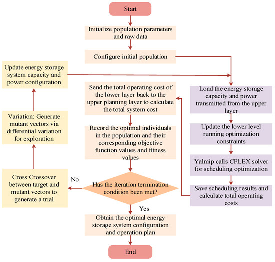
Figure 4.
Solution flowchart.
Step 1: Enter the system’s and the energy storage device’s fundamental parameters, including unit investment cost, unit operation cost, etc., and determine the total number of iterations N. Set the energy storage device’s power and capacity to its initial values for each chromosome.
Step 2: Generate the initial worth of the population and randomly generate the initial population, i.e., the energy storage equipment capacity and power configuration scheme.
Step 3: Pass the generated energy storage device capacity and power from the upper layer to the lower layer, which updates the initial values and constraints.
Step 4: To find the best operating scheme, the lowest layer invokes the CPLEX solver.
Step 5: The top layer receives back the adaption value that corresponds to the equipment’s ideal power result, or the system’s overall operating and maintenance costs, as determined by the bottom layer.
Step 6: After the upper layer obtains the optimal value of the lower layer, it calculates the capacity and power of the upper layer chromosome, i.e., the energy storage device, and obtains the upper layer adaptation value, i.e., the total system cost.
Step 7: Update the optimal values. In the higher-layer model, note and update the global ideal value, as well as the optimal value for each chromosome.
Step 8: Iterative judgment. Verify whether the predetermined maximum number of iterations has been achieved. Proceed to the next step if it has been achieved; if not, go back to Step 2 to continue the iteration.
Step 9: Provide the energy storage device’s ideal configuration.
3. Case Studies
3.1. Database
The study object for case analysis in this work is a wind–solar–thermal complementary power generating system in a particular area. Two thermal power units make up the system, and Table 1 lists the fundamental characteristics of each unit. The solar and wind power plants each have an installed capacity of 250 MW. set at 70 CNY/ton CO2, based on recent data from the China Carbon Market. set at 685 CNY/ton, reflecting the national average thermal coal price published by the National Energy Administration. taken as 0.997 ton CO2/MWh, which corresponds to standard emission factors for coal-fired generation in Chinese grid statistics.

Table 1.
Parameters of thermal power units.
Figure 5 displays the expected wind and solar power output as well as the expected load output on an average day. Table 2 displays the wind, solar, and load membership characteristics [31]. The curtailment penalty values (545 CNY/MWh for solar; 512 CNY/MWh for wind) are based on values used in market-oriented research and pilot studies reflecting the opportunity costs of curtailed renewable energy in China. Table 3 displays the pertinent energy storage parameters, with a 0.95 confidence level.
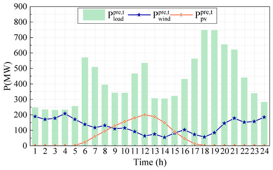
Figure 5.
Typical day wind and solar power and load forecast output.
Table 2.
Trapezoidal fuzzy membership parameters.
Table 3.
Energy storage parameters.
This research establishes three comparison situations to confirm the model’s efficacy.
Scenario 1: Basic scenario. The wind–solar–thermal complementary power generation system is not equipped with energy storage, and the wind–solar forecast value is directly input into the model.
Scenario 2: The wind–solar–thermal complementing power generating system has an energy storage setup, and the wind–solar forecast value is also directly input into the model.
Scenario 3: For the wind–solar–thermal complementing power production system, energy storage is set up, source-load output uncertainty is taken into account, and source-load output is represented using fuzzy opportunity constraints.
3.2. Result Analysis
3.2.1. Analysis of Energy Storage Configuration Results
At a confidence level of 0.95, the energy storage configuration results of the three scenarios are displayed in Table 4.
Table 4.
Energy storage configuration results.
Table 4 shows that there is no energy storage setup in Scenario 1. In Scenario 2, the system’s ideal energy storage configuration capacity is 361.29 MWh, configured power is 67.07 MW, and the energy storage investment cost is CNY 40.1069 million per year. The ideal energy storage configuration power in scenario 3 is 72.16 MWh, while the ideal energy storage configuration capacity is 455.30 MWh. Scenario 3, which accounts for source and load uncertainty, raises the energy storage configuration capacity by 94.01 MWh, the energy storage configuration power by 5.09 MW, and the energy storage investment cost by CYN 9.88 million annually in comparison to the deterministic model.
3.2.2. Analysis of System Operation Results
Figure 6, Figure 7 and Figure 8 show the system operation in a typical day under three scenarios. In Scenario 1, thermal power units bear most of the output. From 0:00 to 5:00, wind power was abandoned, since wind power equipment has anti-peaking properties. From 10:00 to 13:00 and 18:00 to 24:00, wind power was abandoned due to deviations in wind power forecast. From 7:00 to 16:00, solar power was abandoned. In the second scenario, the system incorporates energy storage (ESS). The ESS charges when renewable supply exceeds system demand, specifically during 0:00–4:00 and 9:00–19:00. Conversely, it discharges when electricity demand surpasses conventional generation capacity, specifically during 6:00–8:00, 11:00–12:00, and 17:00–21:00. This reduces the amount of wind and solar power abandoned to a certain extent and alleviates the peaking pressure of thermal power units. However, the uncertainty of source and load output still causes energy waste. Configuring energy storage capacity in Scenario 3 based on source and load output uncertainty makes more sense. The system only has a small amount of wind abandonment during the period between 0:00 and 4:00, and no solar power abandonment occurs. Table 5 shows the description of the legend in Figure 6, Figure 7 and Figure 8.
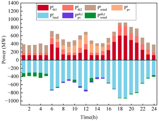
Figure 6.
Scenario 1 operation diagram.
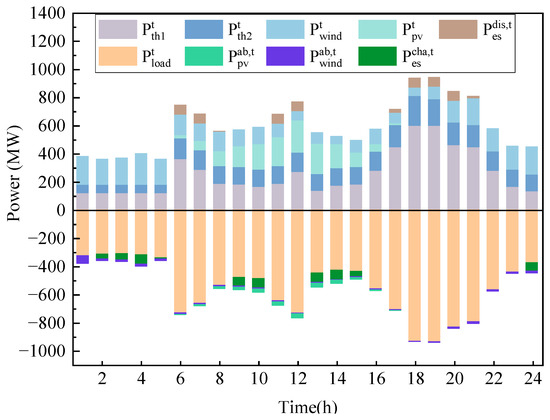
Figure 7.
Scenario 2 operation diagram.
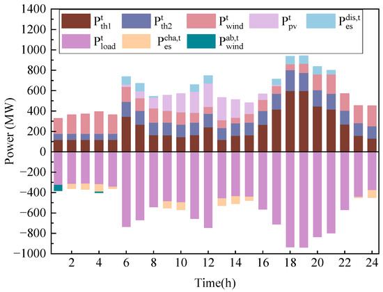
Figure 8.
Scenario 3 operation diagram.
Figure 9 illustrates the total impact on the system under different scenarios. Compared to Scenario 1 without energy storage, the proportion of thermal power generation in Scenarios 2 and 3, which incorporate energy storage, significantly decreased from 69.17% to 65.81% and 62.69%, respectively. The deployment of energy storage reduces the curtailment rates of wind and solar power from 19.68% in Scenario 1 to 1.40% in Scenario 3. This indicates that energy storage effectively reduces reliance on thermal power and enhances the overall integration level of renewable energy.
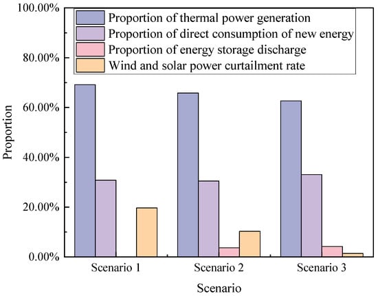
Figure 9.
Total daily impact in different scenarios.
Figure 10 shows that the proportion of the new-energy installed capacity has a non-linear impact on energy storage demand, with accelerated growth. When the proportion of new energy is 35.71%, energy storage requires 72.16 MW of power and 455.30 MWh of capacity. If the proportion of new energy increases to 40%, energy storage demand grows by 48% to 107.36 MW of power and 676.37 MWh of capacity; when the share further increases to 47.05%, the energy storage configuration rises to 180.25 MW of power and 1135.58 MWh of capacity, representing a 150% increase from the baseline level. The results indicate that, once the share of new energy exceeds 40%, each additional percentage point increase triggers a non-linear acceleration in energy storage demand, leading to a significant rise in system balancing costs.
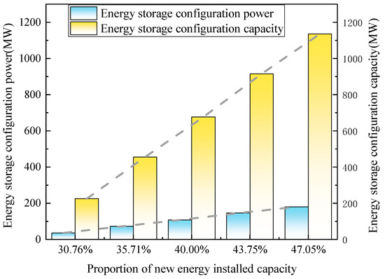
Figure 10.
Sensitivity analysis.
3.2.3. Analysis of System Economic and Environmental Benefits
Table 6 shows indicators such as wind and solar power curtailment rates, carbon emission reductions, system operating costs, and total system costs under the three scenarios.
Table 6.
Related indicators for each scenario.
When comparing Scenarios 1 and 2, we can observe that the energy storage design lowers the system’s overall cost by 13,706.94 × 104 CNY/year, or 10.76%, when compared to the basic scenario. The system operating cost is reduced by 17,717.63 × 104 CNY/year, a decrease of 13.90%, the wind and solar power abandonment rate is reduced by 9.36%, and carbon emissions are reduced by 6.05%.
In contrast to the deterministic model, it is clear from comparing Scenarios 2 and 3 that the system operation model taking into account fuzzy opportunity constraints results in the lowest system comprehensive cost, operation cost, thermal power unit coal consumption cost, wind and solar power abandonment rate, and carbon emissions. In comparison to Scenario 2, Scenario 3’s overall cost is lower by 10,124.42 × 104 CNY/year, or 8.9%, and the system operation cost is lower by 11,112.00 × 104 CNY/year, or 10.13%. Additional improvements have been made to the phenomenon of wind and solar power abandonment, which has decreased by 8.92%. A decrease of 3.51%, or 116,553.93 t, in carbon emissions is achieved. The system meets the expectations of the scheduling decision makers by satisfying the power balance relationship at a confidence level of 0.95 during the scheduling process, demonstrating that the fuzzy opportunity constraint model employed in this paper is not restricted to the absolute equality relationship between the source and the load. As a result, the fuzzy opportunity constraint scheduling model presented in this study has a greater range of optimization, better economy, and lower carbon emissions and abandonment of wind and solar generation.
In conclusion, the energy storage configuration and operation optimization model of the wind–solar–thermal complementary power generation system, which carefully considers fuzzy opportunity constraints, can be used to configure the energy storage capacity in a way that is reasonable, effectively reduces system operating costs, increases the use of new energy, and reduces carbon emissions. This aligns with the development strategy of the power industry, which emphasizes low-carbon, emission reduction, energy conservation, and environmental protection.
3.3. Algorithm Performance Comparison
In order to rigorously evaluate the effectiveness of the differential equation (DE) algorithm relative to other mature meta-heuristic algorithms, we conducted a comparative study that included DE and genetic algorithms (GA). Each algorithm was run for 200 iterations with a population size of 50 individuals, and each experiment was independently repeated 30 times to assess its robustness.
Figure 11 shows the average convergence curves of each algorithm. The differential equation (DE) algorithm reaches the final target value at the 69th iteration, while the genetic algorithm (GA) requires approximately 100 iterations. This indicates that, in our two-layer optimization problem, the DE’s rate-position update mechanism enables a faster global search and accelerates the convergence process.
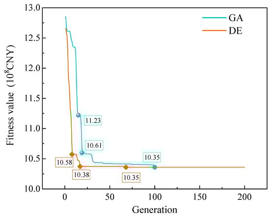
Figure 11.
Comparative convergence behavior of DE and GA.
To examine the stability of the solutions, Table 7 shows the statistical distribution of the final target values in 30 runs. Compared to the genetic algorithm (GA), the differential equation (DE) has the narrowest interquartile range (IQR = 0.03), while the IQR of GA is 0.06, indicating that DE has better consistency when faced with random initialization. Additionally, the best and worst results of DE are within ±0.02 to ±0.03 around the median, whereas GA’s range is ±0.04, further highlighting the robustness of PSO.
Table 7.
Robustness comparison of DE and GA.
The results confirm that DE can achieve faster convergence and more stable solutions at a lower computational cost, making it an ideal solver for the proposed two-layer model.
4. Conclusions
Given the unpredictability of high-proportion renewable energy supply and load output instability, this article carefully analyzes the costs of system operation and energy storage investment. After that, it recommends a two-layer energy storage optimization configuration model that takes source and load uncertainty into consideration. Below are the main conclusions.
The wind–solar–thermal complementary energy system integrates long-term energy storage planning with a short-term operation strategy through internal and external optimization to achieve an optimal energy storage configuration scheme that takes into account both economic and environmental benefits, is conducive to the deep integration of “source-load-storage” resources, and can provide guiding suggestions for long-term power system energy storage planning.
In contrast to the deterministic energy storage configuration model, this work addresses the source-load uncertainty problem using fuzzy chance constraint programming theory. As a result, the energy storage setup is more reliable, and the outcome is more logical. The model proposed in this study reduces the overall cost of the system by 8.9%, operational expenses by 10.3%, wind and solar desertion rates by 8.92%, and carbon emissions by 3.51%.
While the proposed framework demonstrates effectiveness in optimizing energy storage under uncertainty, several issues remain for future research. These include improving forecasting accuracy to enhance uncertainty modeling, reducing the computational burden of the bi-level optimization, and addressing real-time control challenges related to system delays. Furthermore, the evolving nature of policies and markets necessitates flexible and adaptive planning approaches to ensure the long-term viability of energy storage deployment.
Author Contributions
Conceptualization, G.Y.; Data curation, Y.L.; Formal analysis, Z.Z. and W.W.; Investigation, Y.L.; Methodology, G.Y.; Project administration, W.W.; Software, P.Z.; Supervision, W.W.; Validation, P.Z.; Writing—original draft, Y.L. Writing—review and editing, W.W. All authors have read and agreed to the published version of the manuscript.
Funding
This research is supported by State Grid Sichuan Electric Power Company Project: Technical Service for Cost Characteristics Analysis and Comprehensive Benefit Evaluation of Power Grid Engineering under the New Power System of State Grid Sichuan Economic Research Institute in 2024 (B7199624E087).
Data Availability Statement
Data will be made available on request.
Conflicts of Interest
Authors Guangxiu Yu and Ping Zhou were employed by the company State Grid Sichuan Electric Power Company Economic and Technical Research Institute. Author Zhenzhong Zhao was employed by the company State Grid Sichuan Electric Power Company Tianfu New Area Power Supply Company. The remaining authors declare that the research was conducted in the absence of any commercial or financial relationships that could be construed as a potential conflict of interest.
References
- Xi, L.; Shi, Y.; Quan, Y.; Liu, Z. Research on the multi-area cooperative control method for novel power systems. Energy 2024, 313, 133912. [Google Scholar] [CrossRef]
- Wen, L.; Jiang, W. Bi-level capacity optimization of electricity-hydrogen coupled energy system considering power curtailment constraint and technological advancement. Energy 2024, 307, 132603. [Google Scholar] [CrossRef]
- Zhang, Y.; Han, Z.; Tian, B.; Chen, N.; Fan, Y. Coordinated Control Strategy of New Energy Power Generation System with Hybrid Energy Storage Unit. Energy Eng. 2024, 122, 167–184. [Google Scholar] [CrossRef]
- Cao, S.; Dong, Y.; Liu, X. Electromechanical Transient Modeling Analysis of Large-Scale New Energy Grid Connection. Energy Eng. 2024, 121, 1109–1125. [Google Scholar] [CrossRef]
- Wei, D.; He, M.; Zhang, J.; Liu, D.; Mahmud, M.A. Enhancing the economic efficiency of wind-photovoltaic-hydrogen complementary power systems via optimizing capacity allocation. J. Energy Storage 2024, 104, 114531. [Google Scholar] [CrossRef]
- Yang, M.; Wang, J.; Zhou, Y.; Han, G.; Kang, J. Optimal configuration of integrated energy system based on multiple energy storage considering source-load uncertainties under different risk tendencies. J. Energy Storage 2025, 109, 115220. [Google Scholar] [CrossRef]
- Lv, M.; Gou, K.; Chen, H.; Lei, J.; Zhang, G.; Liu, T. Optimal Design of Wind-Solar complementary power generation systems considering the maximum capacity of renewable energy. Energy 2024, 312, 133650. [Google Scholar] [CrossRef]
- Wang, M.; Zhang, B.; Su, B.; Wang, M.; Lv, B.; Zhao, Q.; Gao, H. An multi-timescale optimization strategy for integrated energy system considering source load uncertainties. Energy Rep. 2024, 12, 5083–5095. [Google Scholar] [CrossRef]
- Li, J.; Zhou, Z.; Wen, M.; Huang, H.; Wen, B.; Zhang, X.; Yu, Z. Multi-objective optimization method for medium and long-term power supply and demand balance considering the spatiotemporal correlation of source and load. Energy Strategy Rev. 2024, 54, 101463. [Google Scholar] [CrossRef]
- Tan, M.; Li, Z.; Su, Y.; Ren, Y.; Wang, L.; Wang, R. Dual time-scale robust optimization for energy management of distributed energy community considering source-load uncertainty. Renew. Energy 2024, 226, 120435. [Google Scholar] [CrossRef]
- Zhang, J.; Liu, Z.; Liu, Y. A scheduling optimization model for a gas-electricity interconnected virtual power plant considering green certificates-carbon joint trading and source-load uncertainties. Energy 2025, 315, 134470. [Google Scholar] [CrossRef]
- Liu, Z.; Su, T.; Quan, Z.; Wu, Q.; Wang, Y. Review on the Optimal Configuration of Distributed Energy Storage. Energies 2023, 16, 5426. [Google Scholar] [CrossRef]
- Huang, Q.; Huang, D.K.; Cai, L.; Xu, Q.S. Analysis of optimal configuration of energy storage in wind-solar micro-grid based on improved gray wolf optimization. Sci. Technol. Energy Transit. 2024, 79, 81. [Google Scholar] [CrossRef]
- Lei, S.; He, Y.; Zhang, J.; Deng, K. Optimal Configuration of Hybrid Energy Storage Capacity in a Microgrid Based on Variational Mode Decomposition. Energies 2023, 16, 4307. [Google Scholar] [CrossRef]
- Wu, J.; Xue, L.; Zheng, Y.; Zhang, J.; Li, Q. Operation strategy and capacity configuration of digital renewable energy power station with energy storage. Heliyon 2024, 10, e35181. [Google Scholar] [CrossRef]
- Tian, C.; Liu, M.; Zhang, D.; Liu, F.; Gao, Z. Energy storage optimal configuration in new energy stations considering battery life cycle. Electr. Eng. 2024, 106, 7867–7878. [Google Scholar] [CrossRef]
- Ye, J.; Sha, L.; He, P. Optimization Configuration of Energy Storage Capacity in Wind Solar Storage Combined Power Supply Network Based on Gravity Search Algorithm. In Proceedings of the 2024 3rd International Conference on Energy and Electrical Power Systems (ICEEPS), Chengdu, China, 17–19 May 2024; pp. 68–71. [Google Scholar] [CrossRef]
- Ma, X.; Deveci, M.; Yan, J.; Liu, Y. Optimal capacity configuration of wind-photovoltaic-storage hybrid system: A study based on multi-objective optimization and sparrow search algorithm. J. Energy Storage 2024, 85, 110983. [Google Scholar] [CrossRef]
- Zheng, F.; Meng, X.; Xu, T.; Sun, Y.; Wang, H. Optimization Method of Energy Storage Configuration for Distribution Network with High Proportion of Photovoltaic Based on Source–Load Imbalance. Sustainability 2023, 15, 10628. [Google Scholar] [CrossRef]
- Huang, H.; Hu, Z.; Xu, S.; Wang, X. Capacity configuration strategy for wind-photovoltaic-battery system based on optimized simulated annealing. Int. J. Low-Carbon Technol. 2024, 19, 73–78. [Google Scholar] [CrossRef]
- Zhao, A.P.; Li, S.; Xie, D.; Wang, Y.; Li, Z.; Hu, P.J.-H.; Zhang, Q. Hydrogen as the nexus of future sustainable transport and energy systems. Nat. Rev. Electr. Eng. 2025, 2, 447–466. [Google Scholar] [CrossRef]
- Lv, D.; Liu, W.; Kong, X.; Song, Y.; Zhang, X.; Ma, T.; Zhang, X.; Liu, H. Dynamic reactive power compensation optimization strategy for distribution networks with distributed generators and energy storage systems. J. Phys. Conf. Ser. 2023, 2655, 012002. [Google Scholar] [CrossRef]
- Ren, X.-Y.; Wang, Z.-H.; Li, M.-C.; Li, L.-L. Optimization and performance analysis of integrated energy systems considering hybrid electro-thermal energy storage. Energy 2025, 314, 134172. [Google Scholar] [CrossRef]
- Gong, L.; Li, Y.; Wang, Y.; Zhang, Y. Study on the peak shaving performance of coupled system of compressed air energy storage and coal-fired power plant. J. Energy Storage 2025, 107, 114954. [Google Scholar] [CrossRef]
- Chen, J.; Li, X.; Jing, Y.; Zheng, X.; Deng, J.; Wang, Y.; Wang, K.; Hu, Y. Optimal configuration model of energy storage system and renewable energy based on a high proportion of photovoltaic power. J. Phys. Conf. Ser. 2023, 2495, 012010. [Google Scholar] [CrossRef]
- Ma, Y.; Yu, L.; Zhang, G.; Lu, Z.; Wu, J. Source-load uncertainty-based multi-objective multi-energy complementary optimal scheduling. Renew. Energy 2023, 219, 119483. [Google Scholar] [CrossRef]
- Kevin, W.; Faegheh, M.; Javad, K.; Arindam, B. Economic dispatch of offshore renewable energy resources for islanded communities with optimal storage sizing. Renew. Energy 2025, 241, 122153. [Google Scholar] [CrossRef]
- Li, J.; Liu, K.; Xu, D.; Gao, W.; Huang, L.; Wu, H.; Hua, H. Bi-level optimization for external response of multi-energy complementary micro-energy network based on shared energy storage station. Electr. Power 2025, 58, 43–56. [Google Scholar]
- Tiwari, R.S.; Sharma, J.P.; Gupta, O.H.; Sufyan, M.A.A. Extension of pole differential current based relaying for bipolar LCC HVDC lines. Sci. Rep. 2025, 15, 16142. [Google Scholar] [CrossRef] [PubMed]
- Gao, J.; Meng, Q.; Liu, J.; Yan, Y.; Wu, H. Multi-energy cooperative optimal scheduling of rural virtual power plant considering flexible dual-response of supply and demand and wind-photovoltaic uncertainty. Energy Convers. Manag. 2024, 320, 118990. [Google Scholar] [CrossRef]
- Wang, C.; Tang, Z.; Wei, M.; Liu, X.; Cui, H. Coordinated optimal scheduling of virtual power plants containing wind power and waste-to-energy CHP considering source-load uncertainties. J. Electr. Power Sci. Technol. 2024, 39, 232–241. [Google Scholar] [CrossRef]


Disclaimer/Publisher’s Note: The statements, opinions and data contained in all publications are solely those of the individual author(s) and contributor(s) and not of MDPI and/or the editor(s). MDPI and/or the editor(s) disclaim responsibility for any injury to people or property resulting from any ideas, methods, instructions or products referred to in the content. |
© 2025 by the authors. Licensee MDPI, Basel, Switzerland. This article is an open access article distributed under the terms and conditions of the Creative Commons Attribution (CC BY) license (https://creativecommons.org/licenses/by/4.0/).