Article

Shuffled Puma Optimizer for Parameter Extraction and Sensitivity Analysis in Photovoltaic Models

Department of Green Energy and Information Technology, National Taitung University, Taitung 950309, Taiwan
*
Author to whom correspondence should be addressed.
Energies 2025, 18(15), 4008; https://doi.org/10.3390/en18154008
Submission received: 30 June 2025 / Revised: 19 July 2025 / Accepted: 24 July 2025 / Published: 28 July 2025

Abstract

Photovoltaic (PV) systems are the core technology for implementing net-zero carbon emissions by 2050. The performance of PV systems is strongly influenced by environmental factors, including irradiance, temperature, and shading, which makes it difficult to characterize the nonlinear and multi-coupling behavior of the systems. Accurate modeling is essential for reliable performance prediction and lifespan estimation. To address this challenge, a novel metaheuristic algorithm called shuffled puma optimizer (SPO) is deployed to perform parameter extraction and optimal configuration identification across four PV models. The robustness and stability of SPO are comprehensively evaluated through comparisons with advanced algorithms based on best fitness, mean fitness, and standard deviation. The root mean square error (RMSE) obtained by SPO for parameter extraction are 8.8180 × 10⁻⁴, 8.5513 × 10⁻⁴, 8.4900 × 10⁻⁴, and 2.3941 × 10⁻³ for the single diode model (SDM), double diode model (DDM), triple diode model (TDM), and photovoltaic module model (PMM), respectively. A one-factor-at-a-time (OFAT) sensitivity analysis is employed to assess the relative importance of undetermined parameters within each PV model. The SPO-based modeling framework enables high-accuracy PV performance prediction, and its application to sensitivity analysis can accurately identify key factors that lead to reduced computational cost and improved adaptability for integration with energy management systems and intelligent electric grids.

1. Introduction

The long-term use of fossil fuels has caused global warming, leading to rising temperatures and more frequent extreme weather events. In response to these environmental concerns, the International Energy Agency (IEA) proposed a roadmap targeting net zero carbon emissions by 2050, calling for a fundamental transformation of global energy systems [1]. Among renewable energy technologies, PV systems have become a key solution and have gained particular attention due to their ability to generate electricity directly from sunlight without combustion, emissions, or noise. With PV technology rapidly increasing and maturing, the systems have become modular and relatively easy to install and maintain and have seen substantial reductions in cost over the past decade. These features position photovoltaic (PV) systems as a leading contributor to achieving 2050 climate goals.
Despite the rapid adoption and increasing maturity of photovoltaic systems, accurate modeling of electrical behavior under real-world conditions remains a significant challenge. Although the physical structure of photovoltaic modules is well established, manufacturers normally provide limited internal parameter information through datasheets, which restricts precise system characterization. In addition, photovoltaic output is highly sensitive to external environmental factors such as irradiance, temperature, partial shading, and surface soiling. These dynamic influences, combined with the nonlinear and multiparameter nature of the current voltage relationship, increase the complexity of model development. As a result, parameter extraction and model fitting must address both incomplete input data and time-dependent system behavior, especially in the context of system optimization, fault detection, and real-time control [2].
Equivalent circuit models are commonly used to describe the electrical behavior of photovoltaic systems due to structural clarity and modeling authenticity [3]. SDM is the most widely adopted, representing the current–voltage relationship through five parameters under standard conditions. SDM provides basic nonlinear behavior with low computational cost. However, SDM has reduced accuracy under low irradiance or elevated temperature. To consider more effects in PV systems, DDM adds a second diode to express recombination losses, offering better curve relation in varied environmental conditions. TDM further introduces an additional current path to represent the grain boundary effect. Adding more diodes in parallel increases modeling precision but also raises computation cost; therefore, it is essential to achieve an appropriate balance between model complexity and computational efficiency.
In circuit-based modeling, the accuracy of simulation results relies heavily on the precise identification of unknown model parameters in real-time simulation. To address this task, two principal algorithmic approaches have been developed: analytical methods and metaheuristic methods [4]. Analytical methods used direct or iterative techniques for solving nonlinear mathematical expressions derived from the model structure. Common techniques include Newton–Raphson [5], Gauss–Seidel [6], least squares [7,8], piecewise approximation [9], etc. These methods are advanced for improved computational efficiency and suitability for well-defined mathematical problems but often require complete relative information and are prone to local convergence issues. On the other hand, metaheuristic methods approach parameter extraction as a global optimization problem [10,11,12]; the algorithms explore broader search spaces and avoid local optima, enhancing robustness in the presence of noise or multiple objective functions. Metaheuristics are further classified into various families such as physics-based, swarm-based, evolution-based, and human-based strategies [13]. According to the No Free Lunch (NFL) Theorem [14], no single algorithm can consistently outperform others across all types of optimization problems. This demonstrates that algorithm performance is problem-dependent because an optimizer that performs well in one domain may yield suboptimal results in another. Therefore, it is essential to tailor or enhance optimization algorithms based on the specific characteristics of the problem, such as search space complexity, constraint structure, or convergence requirements. In the context of PV modeling, numerous studies have employed various algorithms for parameter extraction, including differential evolution (DE) [15], particle swarm optimization (PSO) [16], whale optimization algorithm (WOA) [17], grey wolf optimization (GWO) [18], honey badger algorithm (HBA) [19], coati optimization algorithm (COA) [20], etc.

2. Methodology

Puma Optimizer (PO) is a swarm intelligence algorithm within the metaheuristic framework. It can efficiently find suitable solutions through rapid iterations; however, in some cases, it exhibits limited global search ability [21]. To accurately describe the behavior of a commercial photovoltaic system, this study employs a novel metaheuristic algorithm called shuffled puma optimizer (SPO). The approach enhances the global search capability of PO by a mutation strategy. SPO is applied to effectively extract the parameters of PV systems and to evaluate algorithm robustness through comparisons with several advanced optimization algorithms. The detailed contributions and research framework are presented below. Figure 1 illustrates the research flowchart.

2.1. Contribution

  • Proposed a novel algorithm called SPO with a shuffle-mutation strategy to improve the global search capability of PO while maintaining population diversity.
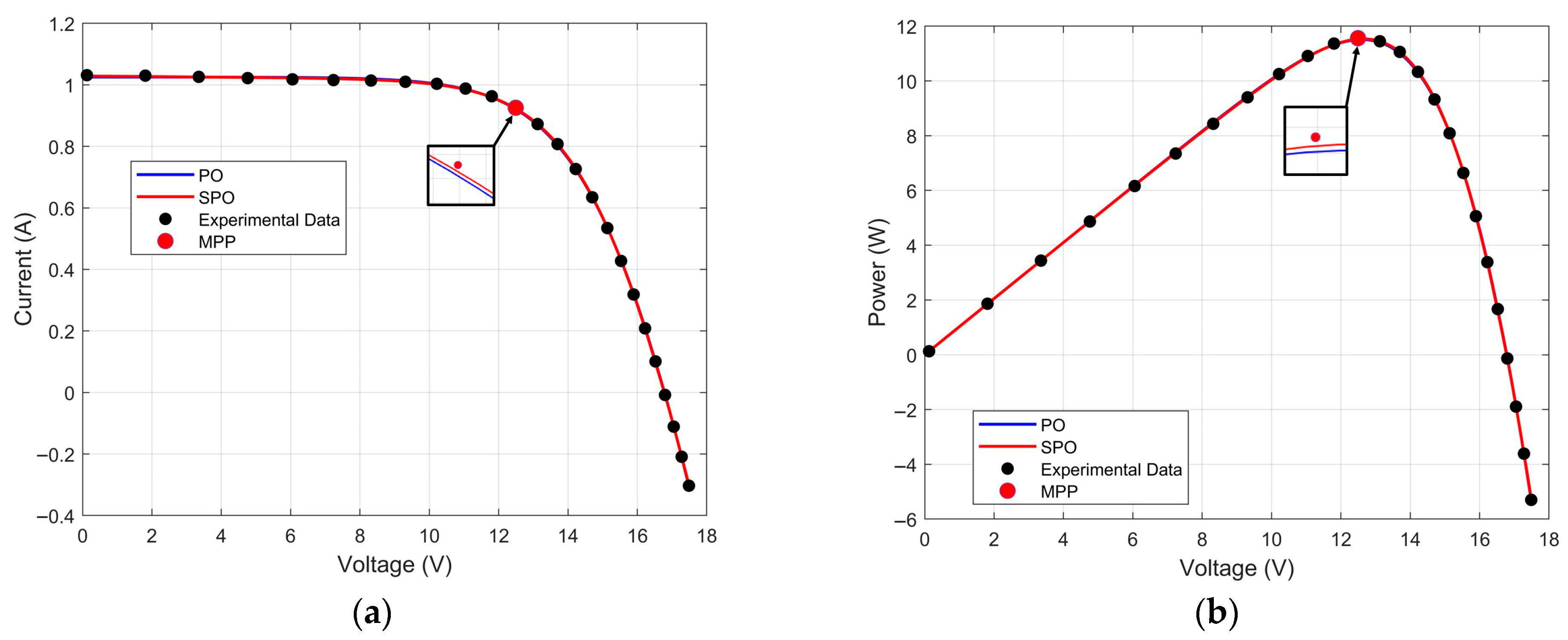
  • Applied SPO to accurately extract parameters for four photovoltaic models: SDM, DDM, TDM, and PMM.
  • A comparative performance analysis of SPO against multiple advanced algorithms using metrics including best fitness, mean fitness, and standard deviation.
  • Performed OFAT sensitivity analysis to identify the influence of individual parameters and determine the key factors in each PV model.

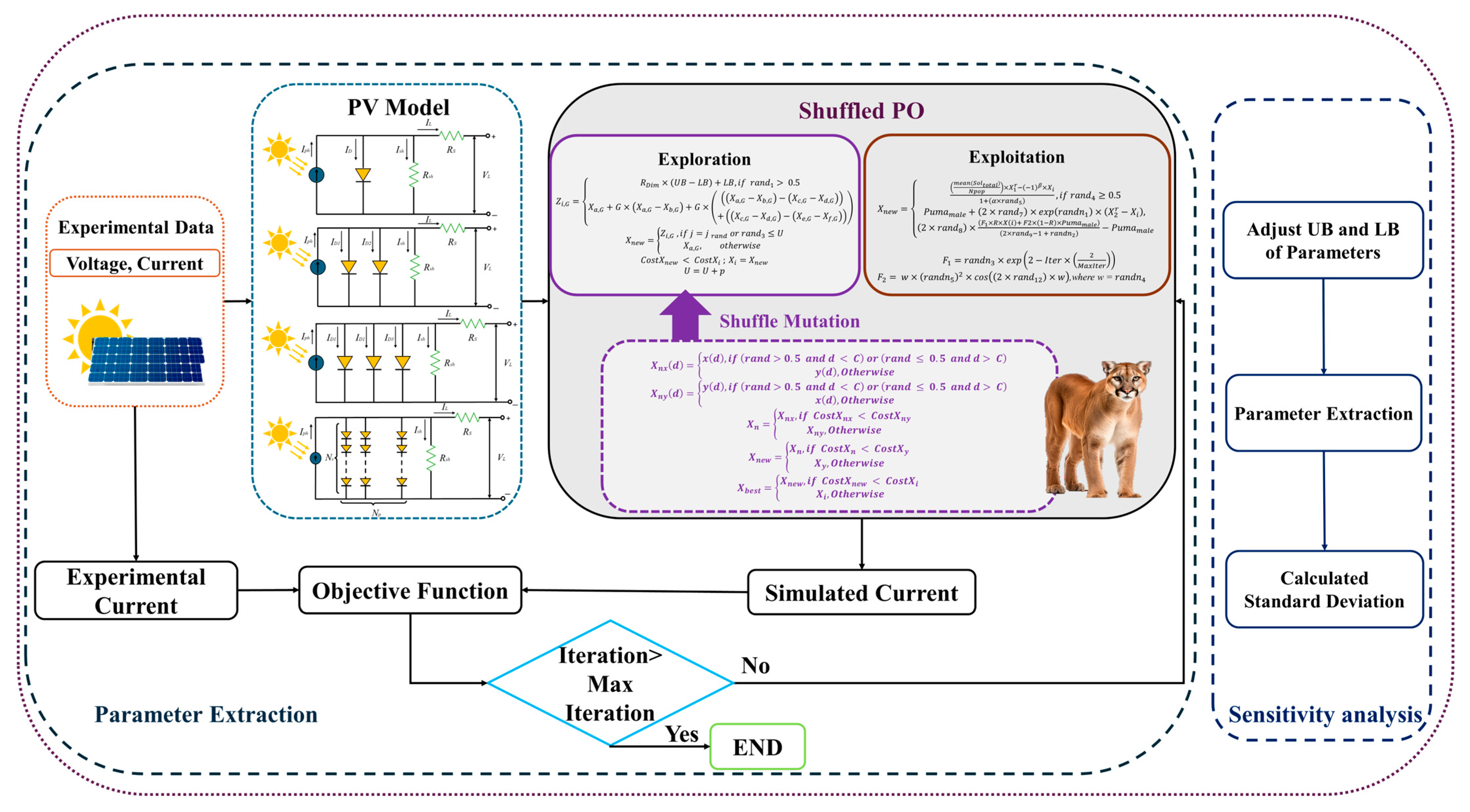
2.2. Research Framework

  • Detailed experimental data collected from the PV system.
  • Built multi-diode models to represent the behavior of the PV system.
  • Enhanced Puma Optimizer with mutation-shuffle strategy.
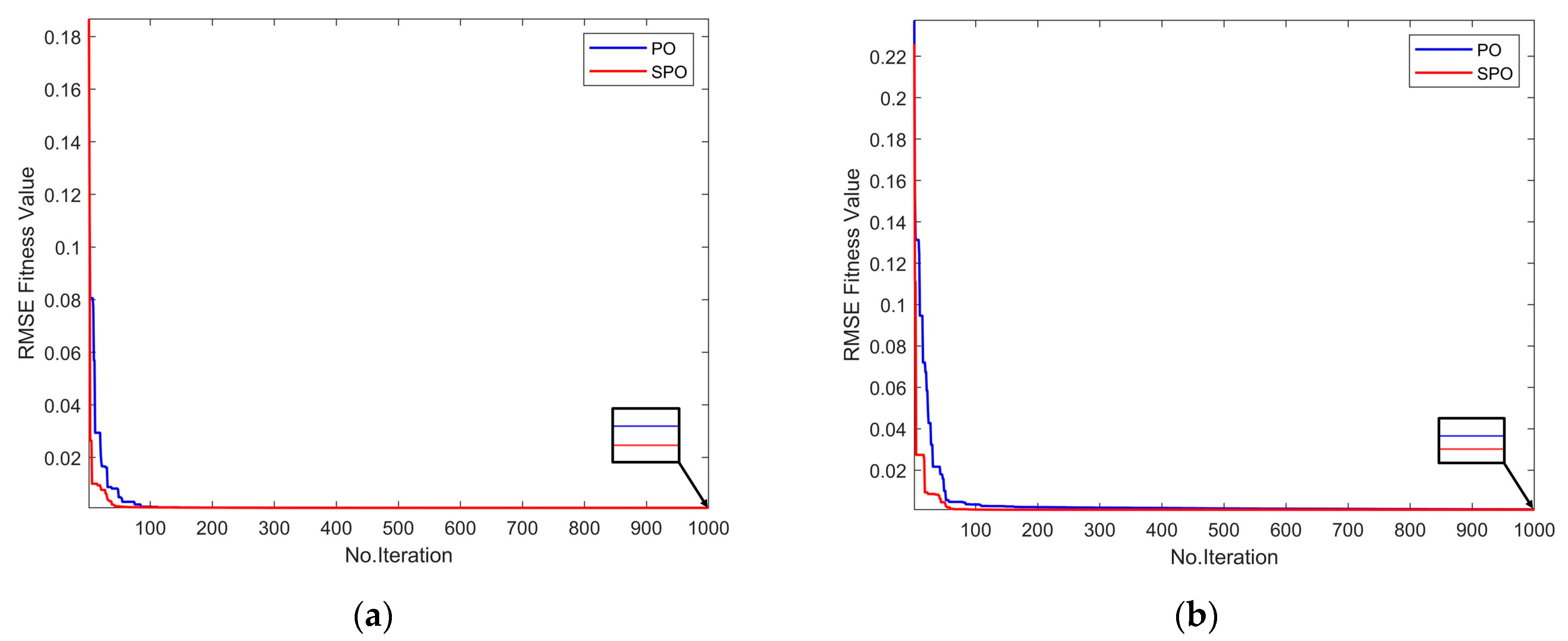
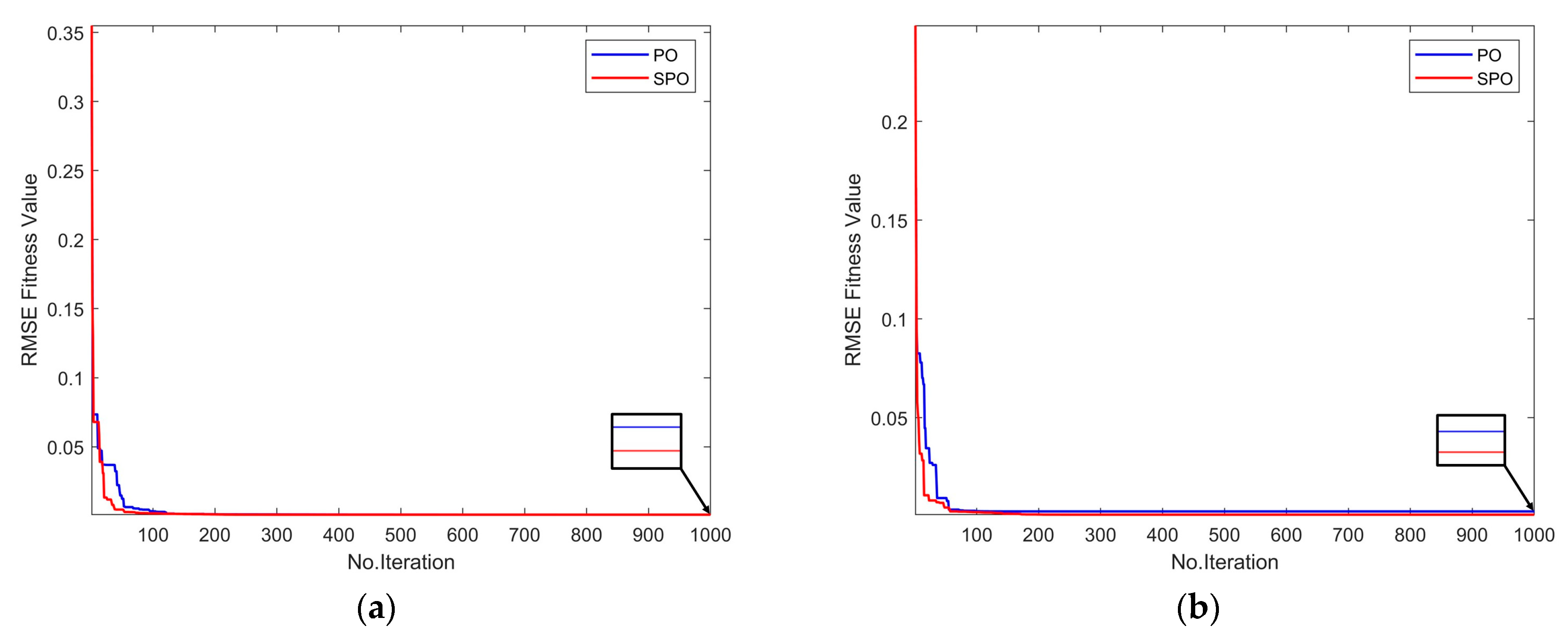
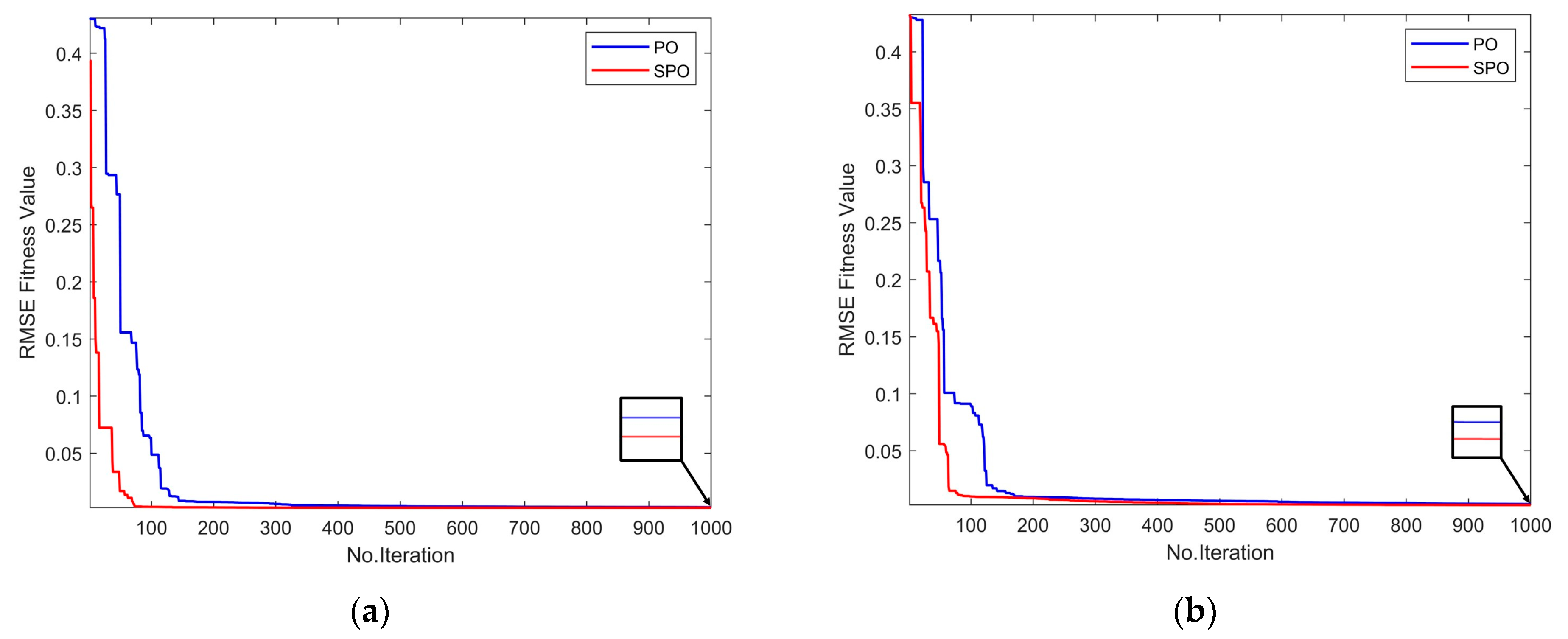
  • Using SPO to extract PV model parameters and analyze the algorithm’s robustness in RMSE.
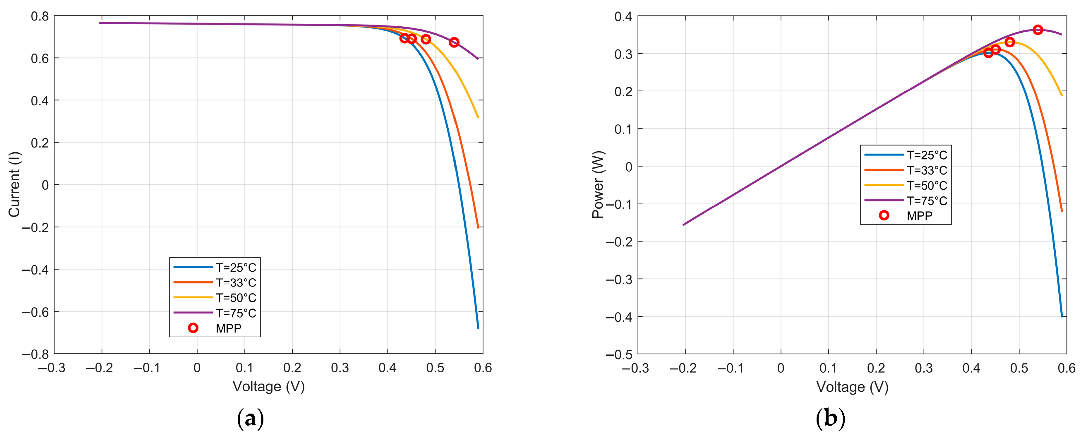
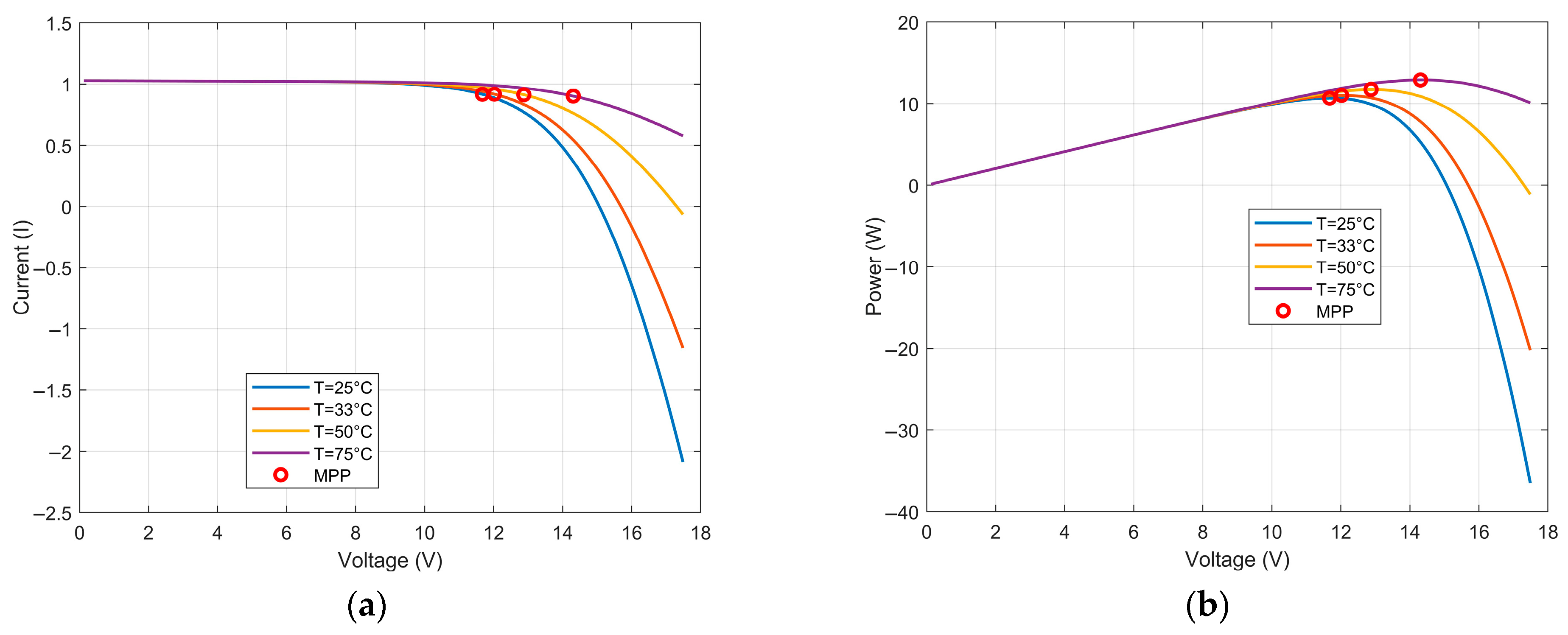
  • Predict PV system performance and maximum power point under four different temperature conditions.
  • Use the OFAT method to analyze key parameters in PV models.

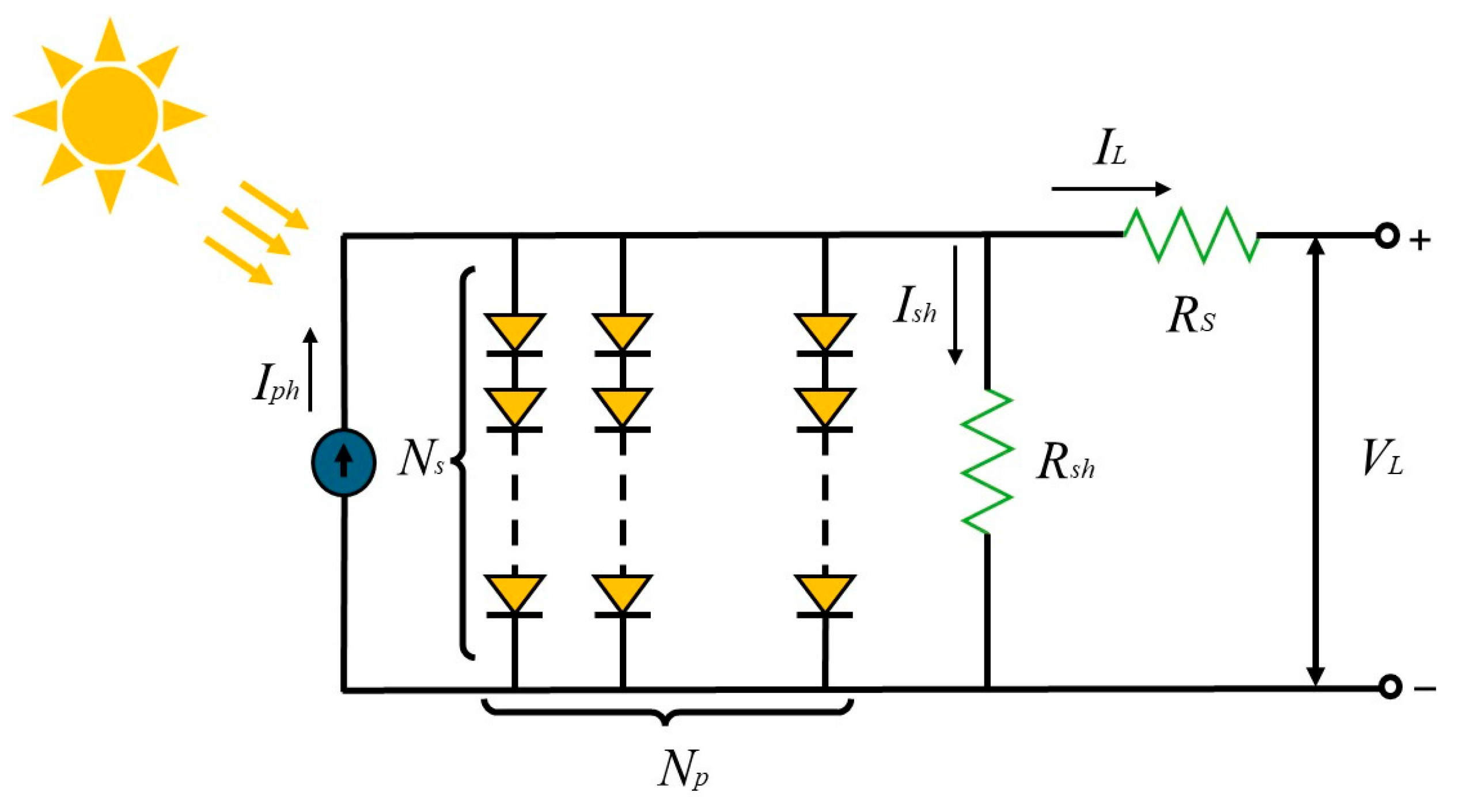
2.3. Photovoltaic System Modeling

Mathematical modeling is essential for fully describing photovoltaic system power characteristics. PV is innately a lighting diode. This section will discuss the single diode model, double diode model, triple diode model, and photovoltaic module model, and further detail the undetermined parameters in each model.

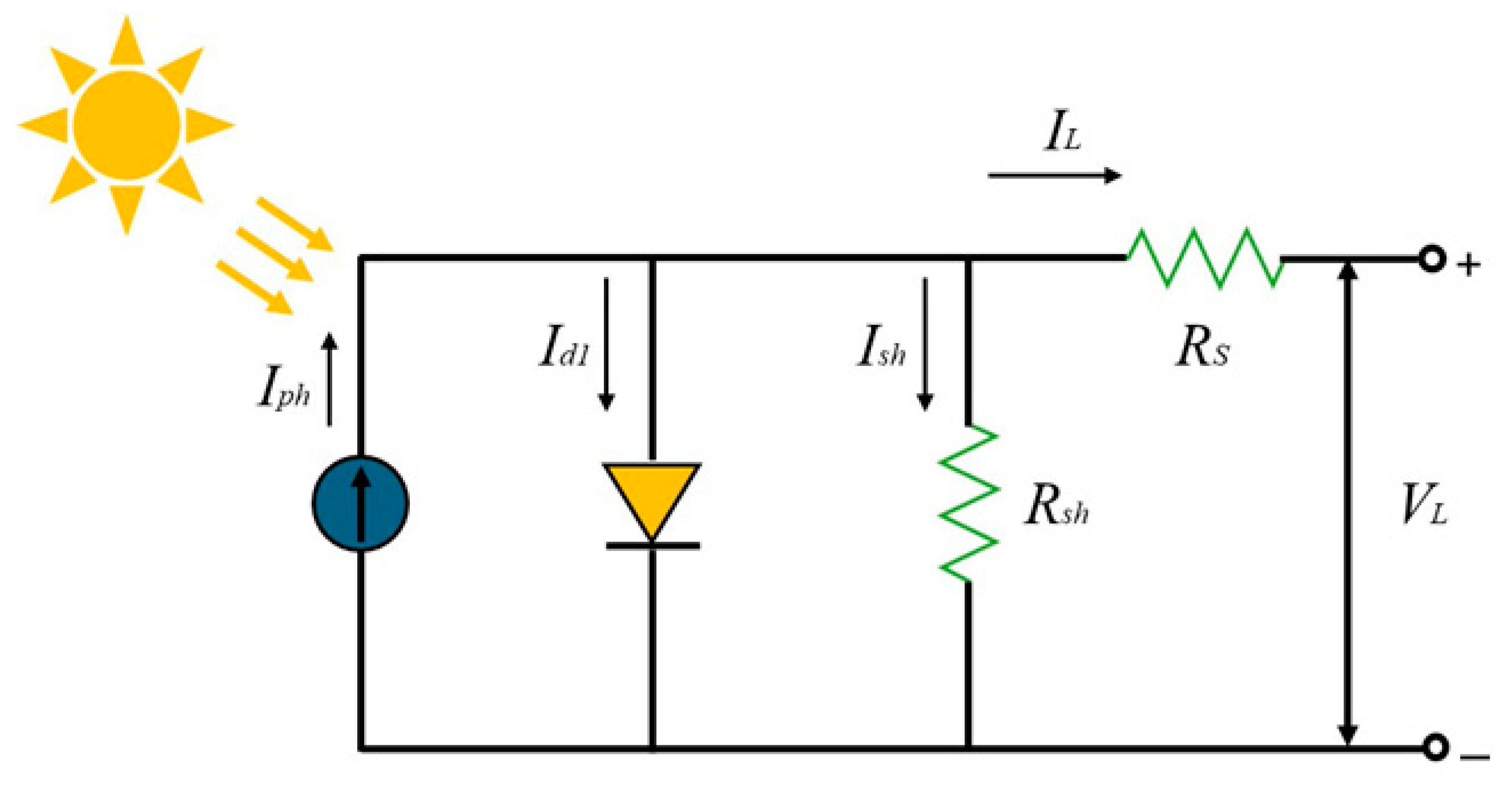
2.3.1. Single Diode Model

SDM is the simplest analog model. It considers the effects of negative doping, internal defects, and leakage current within the PV cell. The equivalent circuit is shown in Figure 2, and the terminal current is calculated as shown in Equation (1), where Iph represents the ideal light-generated current source, Id1 represents the reverse current flowing through the diode due to the diffusion effect, and Ish is the leak current due to the internal defects. Rs is the series resistance, and Rsh is the shunt resistance. The diode reverse current Isd1 is based on the Shockley diode equation, as shown in Equation (2), and Ish is calculated using Equation (3).
I L = I p h I d 1 I s h
I d 1 = I s d 1 exp q V L + I L R s n 1 k T 1
I s h = V L + I L R s R s h
The Isd is the reverse saturation current, q is the elementary charge, and VL and IL represent the terminal voltage and current, respectively. n1 is the diode ideality factor, k is the Boltzmann constant, and T is the absolute temperature in Kelvin. Rs is the series resistance, and Rsh is the shunt resistance. The SDM undetermined parameters are [Iph, Isd1, Rs, Rsh, n1].

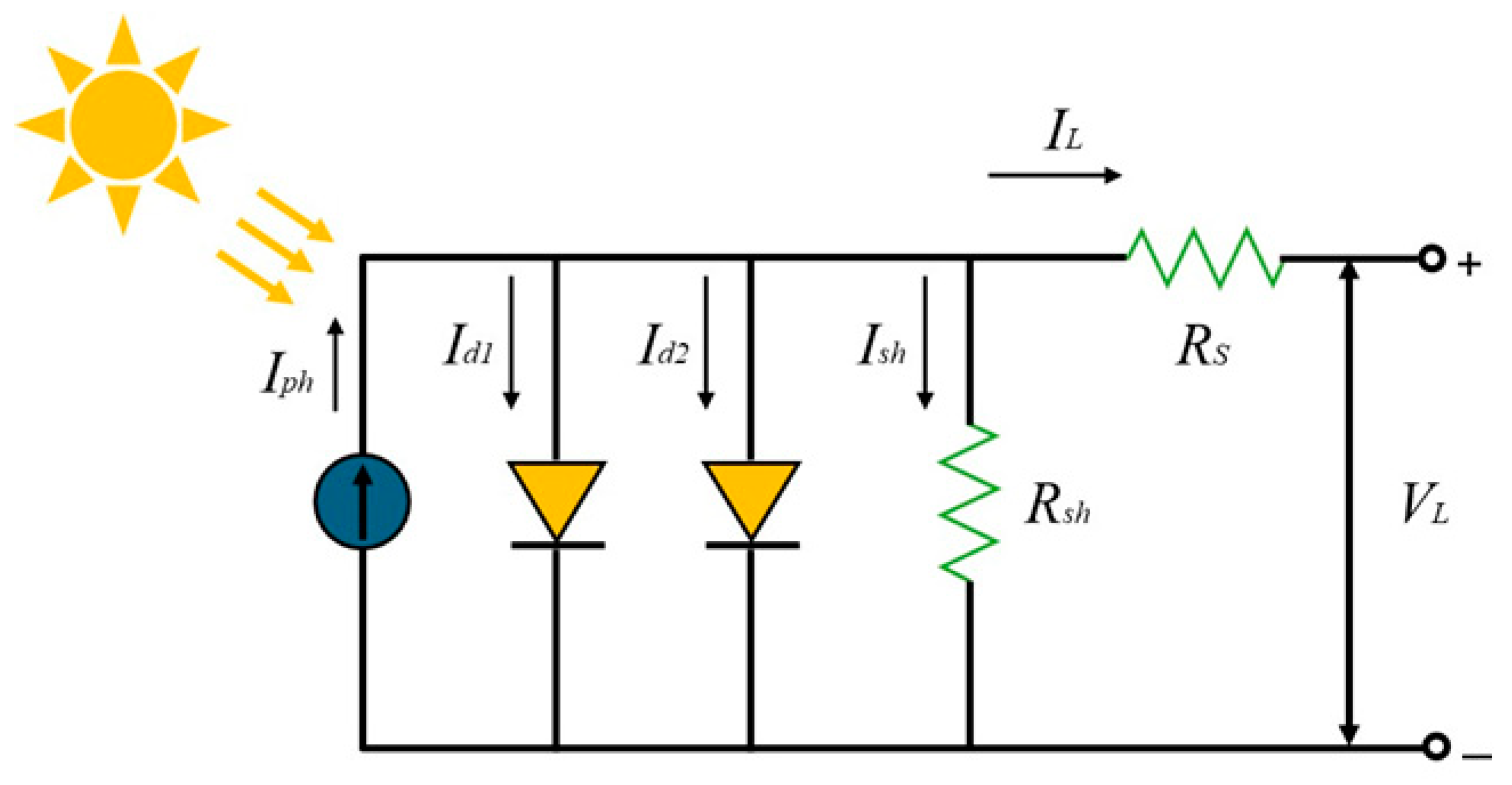
2.3.2. Double Diode Model

Compared with the SDM, the DDM includes an additional shunt diode to account for the recombination effect, especially under low irradiation conditions. The DDM equivalent circuit is shown in Figure 3, and the terminal current IL is expressed by Equation (4).
I L = I p h I d 1 I d 2 I s h
Id1 and Id2 are expressed by Equations (5) and (6), and Ish is shown in Equation (3).
I d 1 = I s d 1 e x p q V L + I L R s n 1 k T 1
I d 2 = I s d 2 e x p q V L + I L R s n 2 k T 1
where Isd1 and Isd2 represent the reverse saturation currents due to diffusion and recombination effects, respectively. n1 and n2 are the diode ideality factors. The DDM undetermined parameters are [Iph, Isd1, Isd2, Rs, Rsh, n1, n2]; the equivalent circuit is shown in Figure 3.

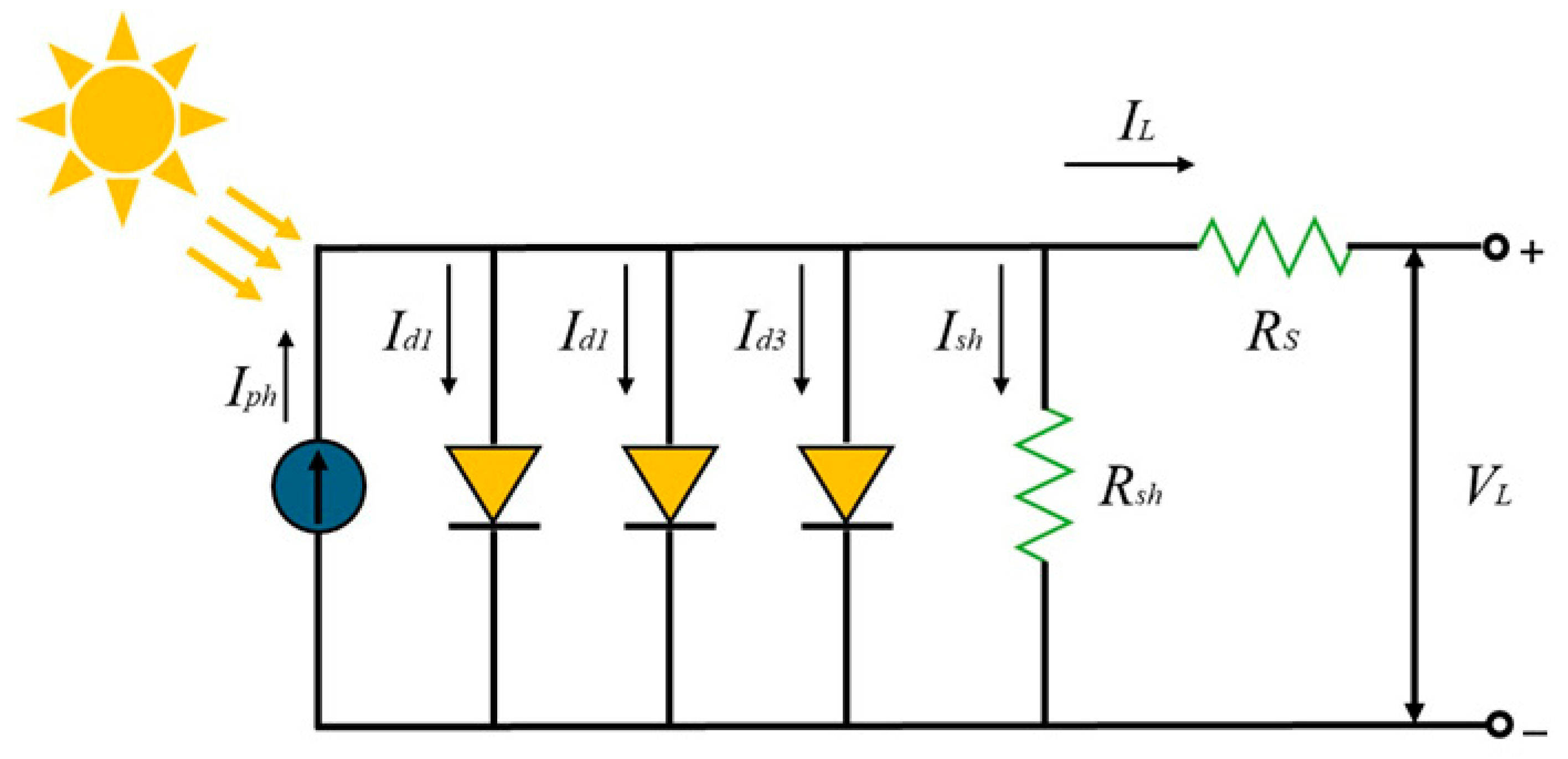
2.3.3. Triple Diode Model

TDM additionally considers the leak current by grain boundary recombination, typically observed in polycrystalline cells. The TDM output IL is expressed in Equation (7).
  I L = I p h I d 1 I d 2 I d 3 I s h
The Id1, Id2, and Id3 are expressed in Equations (8)–(10), respectively. Ish is the same as in Equation (3).
I d 1 = I s d 1 exp q V L + I L R s n 1 k T 1
    I d 2 = I s d 2 exp q V L + I L R s n 2 k T 1
I d 3 = I s d 3 exp q V L + I L R s n 3 k T 1
where Isd3 represents the reverse saturation current due to grain boundary recombination, and n3 is the ideality factor of the third diode. The TDM undetermined parameters are [Iph, Isd1, Isd2, Isd3, Rs, Rsh, n1, n2, n3], and the equivalent circuit is shown in Figure 4.

2.3.4. Photovoltaic Module Model

PMM represents multiple PV cells connected in series and parallel to form a PV module. The terminal IL of the module is expressed in Equation (11).
I L = I p h N p I s d 1 N p exp q V L / N s + I L R s / N p n 1 k T 1 V L N p / N s + I L R s R s h
where Np and Ns are represents the numbers of PV cells connected in parallel and series, respectively. Similar to SDM, PMM has five undetermined parameters [Iph, Isd1, Rs, Rsh, n1], and its equivalent circuit is shown in Figure 5.

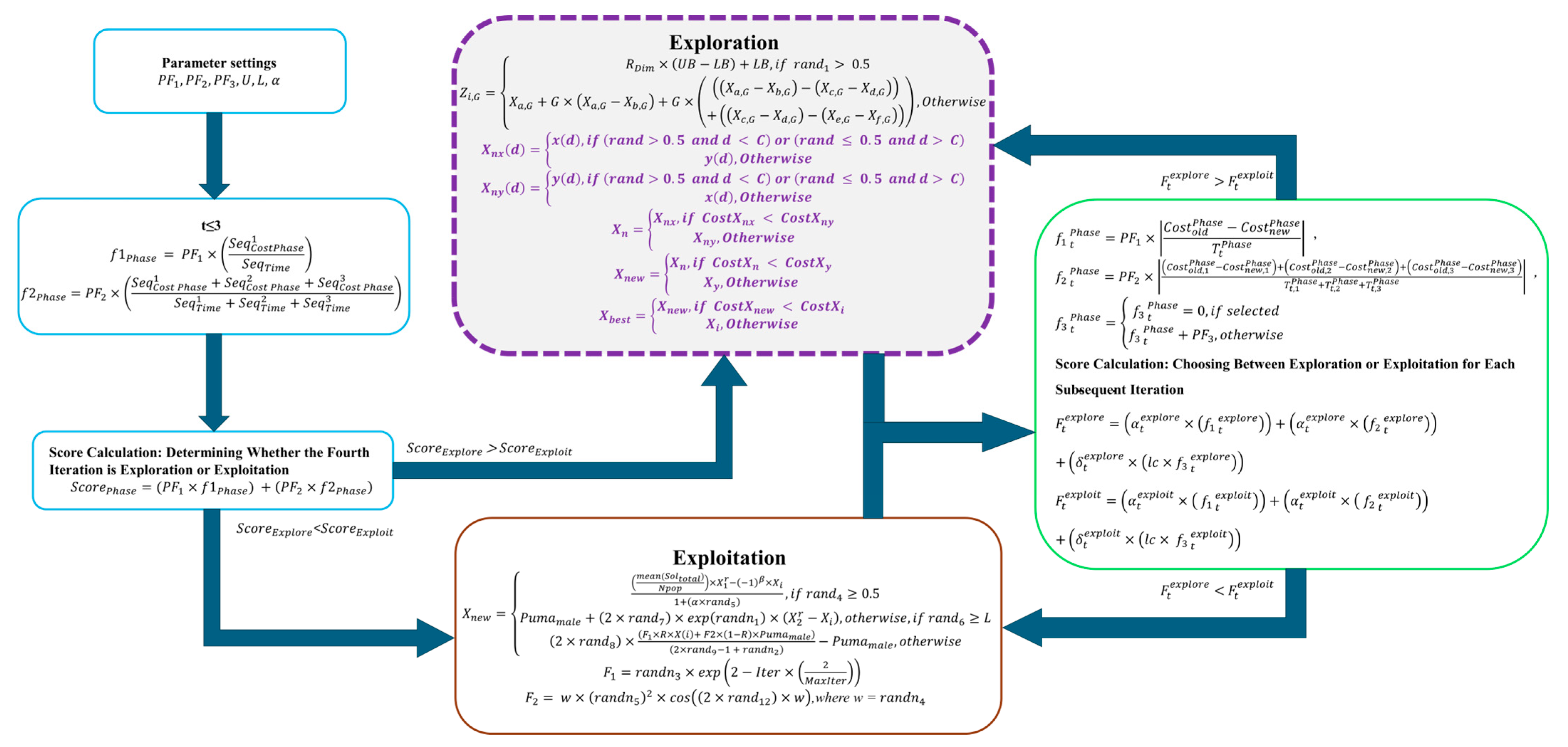
2.4. Shuffled Puma Optimizer

PO is created based on the intelligence and behavioral patterns of pumas [21]. The algorithm has a strong search mechanism in both the exploration and exploitation phases. It also features a flexible switching mechanism between the two phases based on a scoring system, which dynamically balances their ratio to prevent the algorithm from being trapped in local optima. This section will detail the mathematical formulation of the algorithm.

2.4.1. Initialization

The population is defined in Equation (12), where A represents the puma population, Xi is the position of the i-th puma, n is population size, and D is the problem dimension. The puma population is randomly distributed within the search area, as shown in Equation (13).
A = x 1 x 2 x n = x 11 x 12 x 13 x 1 D x 21 x 22 x 23 x 2 D x n 1 x n 2 x n 3 x n D
x i = L B i + r 1 × U B i L B i
where xi is the position of an individual puma, LBi and UBi are the lower and upper bounds of the dimension, respectively, and r1 is a random number between 0 and 1.

2.4.2. Unexperienced Phase

The algorithm performs both exploration and exploitation during the unexperienced phase, as the pumas are not yet familiar with the environment. In each iteration, the puma population will execute two search mechanisms to evaluate the fitness and rank the agents. The best puma position is retained to ensure optimal population evolution. After the first three iterations, the algorithm compares two functions, f1 and f2, to decide which should be executed first in the experienced phase, as shown in Equations (14) and (15). Since the exploration and exploitation phases follow the same execution logic, the variable Phase is defined to represent both phases.
f 1 P h a s e   = P F 1 × S e q C o s t   P h a s e 1 S e q T i m e
f 2 P h a s e = P F 2 × S e q C o s t   P h a s e 1 + S e q C o s t   P h a s e 2 + S e q C o s t   P h a s e 3 S e q T i m e 1 + S e q T i m e 2 + S e q T i m e 3
The f1Phase and f2Phase are the calculation methods for the exploration and exploitation phases. The variables S e q C o s t 1 , S e q C o s t 2 and S e q C o s t 3 represent the calculation results of the two phases in the t-th iteration, as shown in Equations (16)–(18). SeqTime represents that every phase is chosen in every single iteration.
S e q C o s t   P h a s e 1 = C o s t B e s t I n i t i a l C o s t P h a s e 1
S e q C o s t   P h a s e 2 = C o s t B e s t 2 C o s t P h a s e 1
S e q C o s t   P h a s e 3 = C o s t P h a s e 3 C o s t P h a s e 2
In Equations (16)–(18), C o s t B e s t I n i t i a l , C o s t P h a s e 1 , C o s t P h a s e 2 and C o s t P h a s e 3 represent the best fitness values in the initial, first, second, and third iterations, respectively. Equation (19) represents the final score calculation in the unexperienced phase. PF1 and PF2 are constants set to 0.5. The calculation methods for f1Phase and f2Phase are defined in Equations (14) and (15), respectively.
S c o r e P h a s e   = P F 1 × f 1 P h a s e   + P F 2 × f 2 P h a s e  

2.4.3. Experienced Phase

In the experienced phase, the pumas will determine the subsequent execution mode based on the previous experiences. Unlike the unexperienced phase, the experienced phase executes only one of the two phases: exploration or exploitation. After each iteration, the algorithm will evaluate scoring function f1, f2, and f3, incorporating the historical efficiency of exploration and exploitation to ensure the algorithm chooses the best strategy in further iterations. The f1 and f2 functions are presented in Equations (20) and (21), respectively.
f 1 t P h a s e = P F 1 × C o s t o l d P h a s e C o s t n e w P h a s e T t P h a s e
f 2 t P h a s e = P F 2 × C o s t o l d , 1 P h a s e C o s t n e w , 1 P h a s e + C o s t o l d , 2 P h a s e C o s t n e w , 2 P h a s e + C o s t o l d , 3 P h a s e C o s t n e w , 3 P h a s e T t , 1 P h a s e + T t , 2 P h a s e + T t , 3 P h a s e
In the above equations, PF1 and PF2 are constants set to 0.5, C o s t o l d P h a s e denotes the fitness value from the previous iteration of either exploration or exploitation, while C o s t o l d P h a s e presents the best solution obtained in the current iteration. T t P h a s e represents the number of times the corresponding phase has not been selected up to the current iteration. T t , 1 P h a s e , T t , 2 P h a s e , T t , 3 P h a s e are the same concept as T t P h a s e , but correspond to the three historical records from previous iterations. The f3 function is shown in Equation (22):
f 3 t P h a s e = f 3 t P h a s e = 0 , i f   s e l e c t e d     f 3 t P h a s e + P F 3 , o t h e r w i s e  
f 3 t P h a s e is an artificially balanced operator, as only one phase (either exploration or exploitation) is executed in each iteration. If a phase is not selected in a given iteration, a constant value PF3 set to 0.3, is added until that phase is eventually chosen. Equations (23) and (24) present the scoring methods for the exploration and exploitation phases in F t e x p l o r e and F t e x p l o i t , respectively.
F t e x p l o r e = α t e x p l o r e × f 1 t e x p l o r e + α t e x p l o r e × f 2 t e x p l o r e + δ t e x p l o r e × l c × f 3 t e x p l o r e
F t e x p l o i t = α t e x p l o i t ×   f 1 t e x p l o i t + α t e x p l o i t ×   f 2 t e x p l o i t + δ t e x p l o i t × l c × f 3 t e x p l o i t
l c = C o s t o l d C o s t N e w e x p l o i t a t i o n     C o s t o l d C o s t N e w   e x p l o r a t i o n ,   0 l c
α t e x p l o r e ,   e x p l o i t = α e x p l o i t = 0.99 ,   α e x p l o r e = α e x p l o r e 0.01 , 0.01 , i f   F e x p l o i t > F e x p l o r e α e x p l o r e = 0.99 ,   α e x p l o i t = α e x p l o i t 0.01 , 0.01 , O t h e r w i s e
δ t e x p l o r e = 1 α t e x p l o r e
δ t e x p l o i t = 1 α t e x p l o i t
Equations (25)–(28) provide the detailed references in Equations (23) and (24). PO coordinates the f1 and f2 ratio. If the exploitation score is greater than the exploration score, α will decrease linearly, while δ increases to prevent the algorithm from executing more in one phase, avoiding imbalance that may cause the search to diverge or be limited in local optima. l c represents the difference in fitness between the best solutions of the exploration and exploitation modes before and after the current iteration.

2.4.4. Exploration Phase

During the exploration phase, the puma will either move toward a new area or randomly collaborate with other pumas for hunting. The expression is shown in Equation (29).
Z i , G = R D i m × U B L B + L B , i f     r a n d 1 > 0.5   X a , G + G × X a , G X b , G + G × X a , G X b , G X c , G X d , G + X c , G X d , G X e , G X f , G , O t h e r w i s e  
G = 2 × r a n d 2 1
where rand1 and rand2 are the randomly generated values between 0 and 1 and UB and LB represent the upper and lower bounds in the search area, respectively. X a , G , X b , G , X c , G , X d , G , X e , G , X f , G are the solutions of six different pumas in the population. G denotes the direction vector in [−1, 1].
X n e w = Z i , G   ,   i f   j = j r a n d   o r   r a n d 3 U X a , G ,     o t h e r w i s e
N C = 1 U
p = N C N p o p
C o s t X n e w < C o s t X i   ;   X i = X n e w
U = U + p
The new solution is defined in Equation (31). In Equations (32)–(35), Zi,G denotes the newly generated solution, jrand is the randomly selected index within the solution’s dimension, U is a decreasing value between 0 and 1, and Npop represents the number of pumas in the population. If the new cost is smaller than the original cost, the original solution is replaced.

2.4.5. Exploitation Phase

The exploitation phase is inspired by the puma’s running and hunting behavior. The renewed solution is expressed in Equation (36), and the related parameters are calculated as shown in Equations (37)–(41).
X n e w = m e a n S o l t o t a l N p o p × X 1 r 1 β × X i 1 + α × r a n d 5 ,   i f   r a n d 4 0.5 P u m a m a l e + 2 × r a n d 7 × e x p r a n d n 1 × X 2 r X i ,   o t h e r w i s e , i f   r a n d 6 L 2 × r a n d 8 × F 1 × R × X i + F 2 × 1 R × P u m a m a l e 2 × r a n d 9 1 + r a n d n 2 P u m a m a l e , o t h e r w i s e
X 2 r = r o u n d 1 + N p o p 1 × r a n d 10
R = 2 × r a n d 11 1
F 1 = r a n d n 3 × e x p 2 I t e r × 2 M a x I t e r
F 2 = w × r a n d n 5 2 × c o s 2 × r a n d 12 × w
w = r a n d n 4
In Equations (36)–(41), rand4, rand5, rand6, rand7, rand8, rand9, rand10, rand11, and rand12 are randomly generated values between 0 and 1. When rand4 is greater than 0.5, the running behavior is executed; otherwise, a short or long jump is performed depending on the value of rand6. Soltotal is the sum of all solutions, and Npop is the number of pumas in the population. The parameters α and L are constant values set to 2 and 0.67, respectively. r a n d n 1 , r a n d n 2 , r a n d n 3 , r a n d n 4 and r a n d n 5 are randomly generated numbers following a normal distribution. Pumamale is the best candidate solution among all iterations so far. MaxIter is the maximum number of iterations. The values representing the balance between the puma’s recent position and the best position are denoted as F1 and F2, respectively.

2.4.6. A Shuffle Mutation Strategy for Global Optimization

In this section, we introduce the shuffle technique as a novel mutation strategy to enhance the algorithm’s exploration capability. The principle of shuffle mutation involves randomly swapping or rearranging the order of solutions. In each iteration, solutions are first ranked based on fitness, followed by a shuffle operation that disrupts structural patterns and generates more diverse solution sequences. This approach expands the solution distribution, reduces the likelihood of local optima, and avoids premature convergence of the algorithm. The modified mutation and selection mechanisms in the PO are designed to enhance its exploration ability and overall search performance in high-dimensional solution spaces, as shown in Equations (42)–(45).
X n x d = x d , i f   r a n d > 0.5   a n d   d < C   o r   r a n d     0.5   a n d   d > C   y d , O t h e r w i s e   X n y d = y d , i f   r a n d > 0.5   a n d   d < C   o r   r a n d     0.5   a n d   d > C   x d , O t h e r w i s e  
X n = X n x , i f     C o s t X n x < C o s t X n y   X n y , O t h e r w i s e  
X n e w = X n , i f     C o s t X n < C o s t X y   X y , O t h e r w i s e  
X b e s t = X n e w , i f     C o s t X n e w < C o s t X i     X i , O t h e r w i s e  
The mutation and selection processes involve multiple random and conditional operations to enhance search efficiency and solution quality. First, a random number rand is set within the range [0, 1] and used to determine the probability of the swap direction. The crossover point C is a randomly selected index within the solution’s dimensional range, used for subsequence exchange. The current dimension is denoted by d, x represents the current solution, and y is the new solution obtained through exploration.
An alternative mutation mechanism is developed in this study, as shown in Equation (42), to replace the traditional crossover method. When the random number rand is greater than 0.5 and the current dimension is less than the crossover point C, or when rand is less than or equal to 0.5 and the dimension is greater than C, the subsequence before point C is retained from the original solution x, while the subsequence after point C is taken from the newly explored solution y. Otherwise, the subsequence before C is retained from y, and the subsequence after C is taken from x, resulting in the crossover solutions Xnx and Xny. Figure 6 shows the proposed improved mechanism.
In addition, all solutions are subjected to fitness analysis to evaluate their performance in the solution space. Fitness evaluation helps identify potential high-quality solutions. As shown in Equation (43). The two crossover solutions, Xnx and Xny, are initially generated with corresponding costs Xnx and Xny. The algorithm first compares the costs of these two solutions and selects the one with the lower cost as the result Xn, which is then compared with Xy. Equation (44) performs the second-stage comparison between Xn, the result obtained from Equation (43), and the newly explored solution Xy, with corresponding costs CostXn and CostXy. The solution with the lower cost is recorded as Xnew, as shown in Equation (45).
The improved strategy with the shuffle-mutation mechanism can effectively increase population diversity and solution quality. The calculation flow of the SPO is shown in Figure 7.

2.5. Objective Function and Parameter Setting

This section introduces the parameter identification and parameter sensitivity objective functions. The goal of PV modeling is to find the optimal solution by minimizing the difference between the experimental data and the calculated data, as shown in Equation (46).
R M S E = 1 N t = 1 N I c a l c I e x p 2 = 1 N t = 1 N f m o d e l V L , I L , x I t 2
Icalc denotes the calculated current by the algorithm, while Iexp refers to the experimental data of the PV cell or system., N is the number of data points. VL and IL represent the PV terminal voltage and current, respectively. x is the parameter vector defined in Table 1, and f represents the mathematical function of the four PV models.
To extract the physical meaning of the parameters, the algorithm requires a defined search range. Table 2 presents all parameters along with their corresponding identification ranges.
To evaluate the parameter sensitivity of the PV models, this study adopts the OFAT method as the sensitivity objective function, as shown in Equation (47). The sensitivity test is conducted by varying each parameter from 0.8 to 1.2 times its original value. The standard deviation (STD) of the RMSE across the tested range is then calculated to identify the influential parameters in the four models, where RMSEi is the error corresponding to a single parameter and R M S E ¯ is the average error across the entire range of parameter variations.
S T D = 1 M i = 0.8 1.2 R M S E i R M S E ¯ 2
Both the shuffled PO and the original PO were evaluated over 30 independent runs, using 30 agents and 1000 iterations, as shown in Table 3. All simulations were conducted on an Intel i9-01 CPU using MATLAB 2024a.

3. Results and Discussion

To evaluate the adaptability of the shuffled PO in PV parameter optimization, the results are compared with the original PO and several competitive algorithms in terms of best fitness, mean fitness, and standard deviation. After comparing the robustness of the algorithms, the PV performance and maximum power point (MPP) are further predicted under various temperature conditions.

3.1. SDM

In SDM, there are five undetermined parameters. Table 4 shows SPO and PO compared with experimental data. Table 5 presents the comprehensive algorithm estimation results, including best fitness, mean fitness, and standard deviation. The results show that SPO achieves the best search performance in the SDM. Figure 8 shows that SPO has better best and mean convergence speed than the original PO. Figure 9 displays the experimental I–V and P–V curves against SPO and PO. The SPO’s best parameters were then applied to predict the performance in various temperature conditions, as shown in Figure 10.

3.2. Double Diode Model

There are seven undetermined parameters in DDM. Table 6 lists SPO and PO against the experiment at each point. Table 7 is the parameter extraction results; SPO also has better search results in the DDM model. Figure 11 and Figure 12 are the algorithms’ convergence curve and the I–V and P–V curves, respectively. Figure 13 shows SPO predicted performance in different temperature conditions.

3.3. Triple Diode Model

There are nine undetermined parameters in the TDM model. Table 8 shows the calculation results of SPO and PO at each data point. Table 9 presents the robustness results of ten algorithms, including the best, mean, and standard deviation of fitness. The convergence curves and comparison results are shown in Figure 14 and Figure 15. The prediction performance of the TDM model under different temperature conditions is shown in Figure 16.

3.4. Photovolataic Module Model

For PMM parameter extraction, ten algorithms are compared to evaluate the robustness of SPO. Table 10 presents the comparison between experimental data, SPO, and PO at each data point. Table 11 shows the robustness results in terms of best, mean, and standard deviation values. The convergence curves in Figure 17 indicate that SPO achieves better search speed and solution quality than PO. Figure 18 shows the comparison results with experimental data, and Figure 19 illustrates the SPO prediction performance in the PMM model under four different temperature conditions.
The above results indicate that SPO achieves better search performance than PO, as its enhanced global search capability allows for more effective exploration of the solution space and reduces the risk of being trapped in local optima. Table 12 further demonstrates that the improved mutation strategy strengthens the algorithm’s global search ability in PV system parameter extraction.

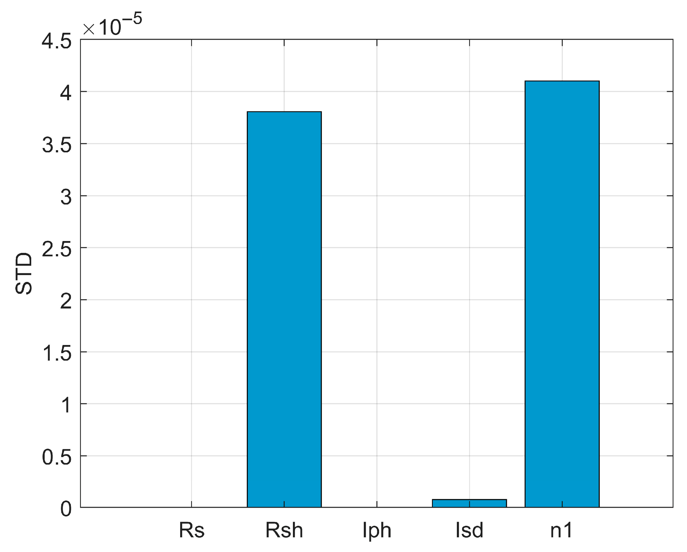
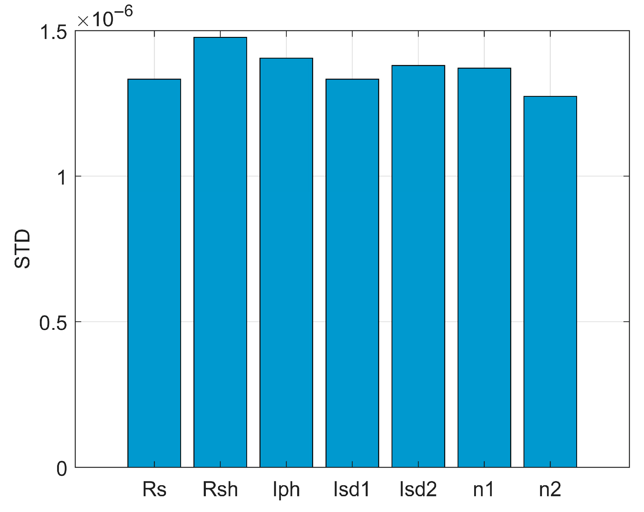
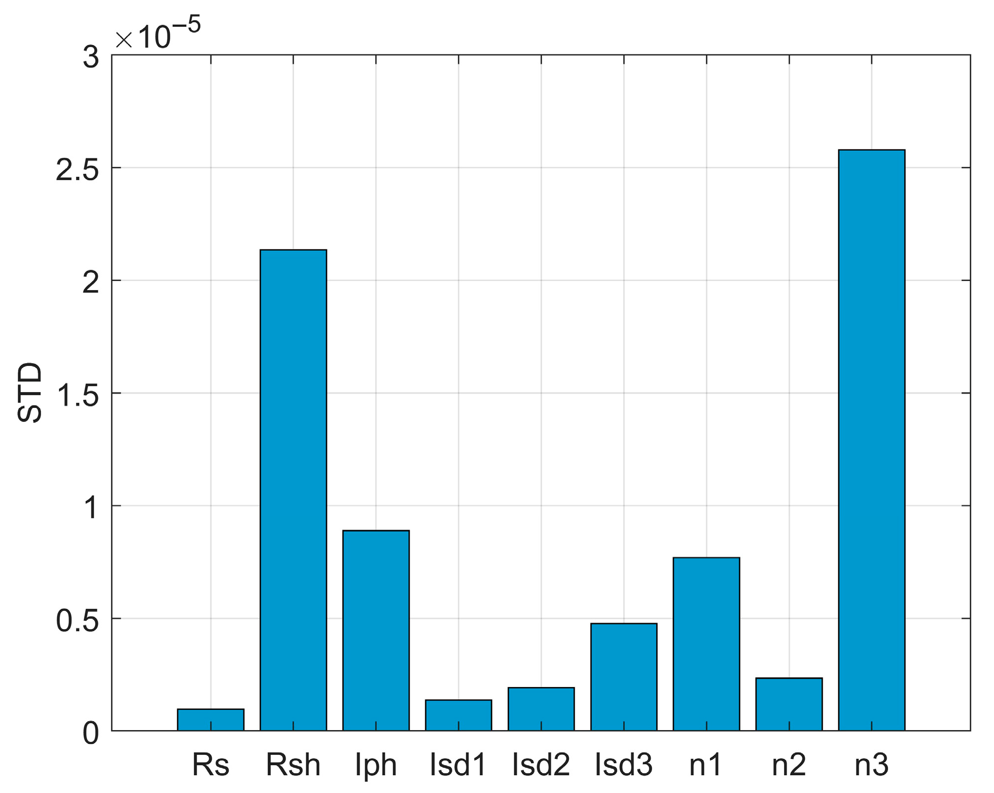
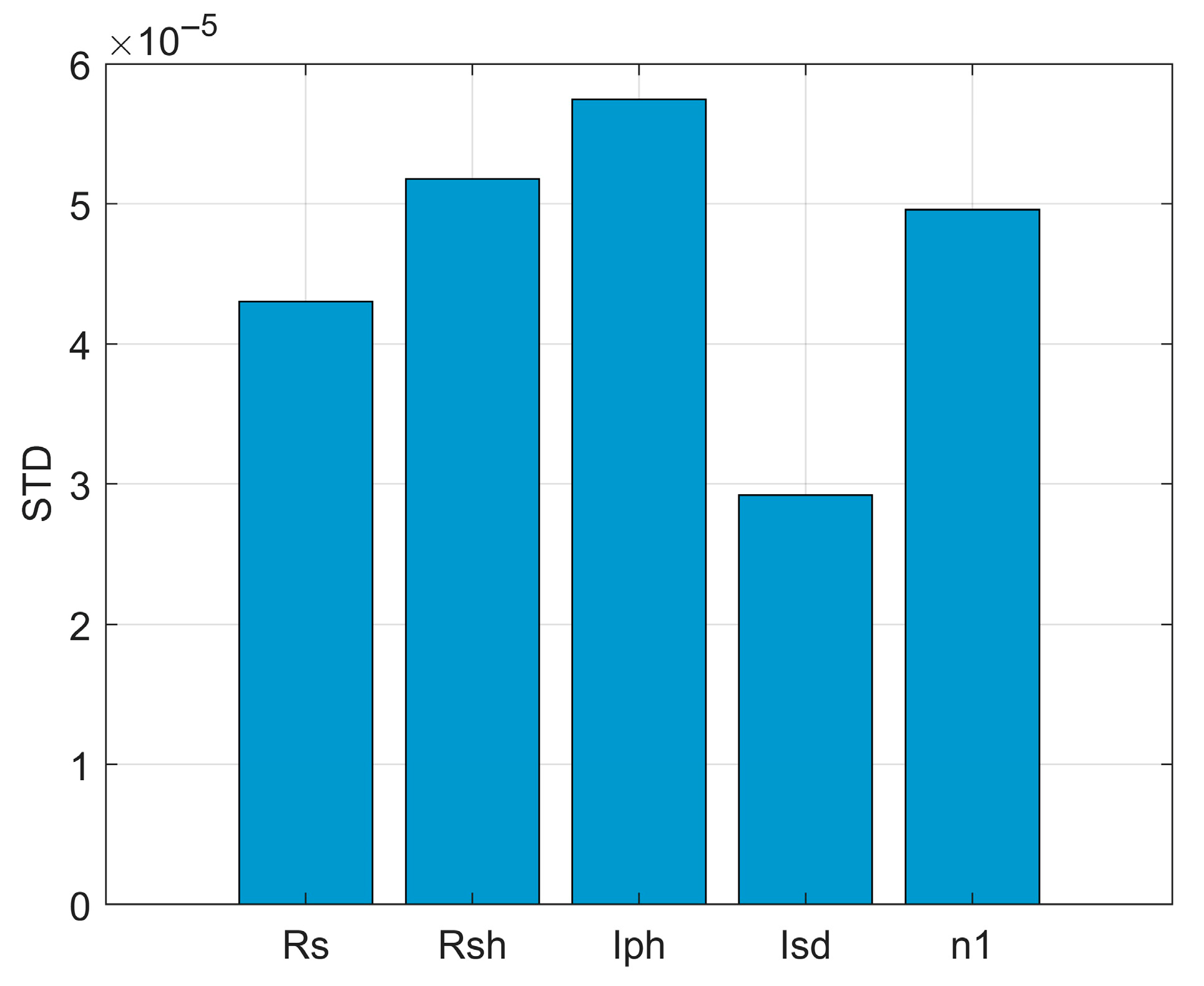
3.5. Sensitivity Analysis

Model complexity affects computational cost. Using fewer parameters to produce a minimized solution offers high adaptability in real-time scenarios. Parameter sensitivity analysis evaluates model robustness under small input variations and supports parameter prioritization, helping manufacturers focus optimization efforts on the most impactful parameters. This research applies the OFAT method to evaluate parameter effectiveness in the SDM, DDM, TDM, and PMM, with results shown in Figure 20, Figure 21, Figure 22 and Figure 23.

4. Conclusions

Limited manufacturer information and the nonlinear characteristics of PV systems hinder accurate performance prediction, MPP identification, and integration with EMS. This study establishes a rigorous benchmark process for accurate PV modeling and conducts a comprehensive analysis to prioritize key model parameters, thereby advancing the precision and reliability of photovoltaic performance prediction. The SPO is proposed for efficient PV model parameter extraction, performance prediction, and sensitivity analysis. The overall results indicate that SPO exhibits stronger global search capability compared to the original PO. To evaluate its robustness in PV system modeling, SPO is compared with several algorithms using best value, mean value, standard deviation, and convergence performance. For the four PV models (SDM, DDM, TDM, and PMM), SPO achieves the lowest objective values, with the best fitness results of 8.8180 × 10⁻⁴, 8.5513 × 10⁻⁴, 8.4900 × 10⁻⁴, and 2.3941 × 10⁻³, respectively. In terms of solution stability, SPO also outperforms PO, with corresponding standard deviations of 3.7924 × 10⁻¹⁷, 9.3500 × 10⁻⁶, 1.6800 × 10⁻⁵, and 1.1942 × 10⁻⁵. Based on the identified optimal parameters, this study predicts the performance of the PV system and MPP under four different temperature conditions. Furthermore, sensitivity analysis identifies shunt resistance as the most influential parameter across all PV models, highlighting that leakage current is an important factor in PV system behavior.
Overall, the results show that accurate parameter estimation combined with sensitivity analysis supports reliable PV modeling by enhancing prediction accuracy and simplifying model structure, making the approach suitable for PV researchers and manufacturers.

Author Contributions

Conceptualization, E.-J.L.; methodology, R.-W.C.; software, Q.-A.W.; validation, W.-L.L.; investigation, R.-W.C.; data curation, Q.-A.W.; visualization, R.-W.C.; writing—original draft, E.-J.L.; project administration, E.-J.L. All authors have read and agreed to the published version of the manuscript.

Funding

All authors gratefully acknowledge the financial support from the National Science and Technology Council under Grant No. 114-2221-E-143-005.

Data Availability Statement

The data that support the findings of this study are available on request from the corresponding author.

Acknowledgments

The author wishes to thank the editor and the reviewers for their insightful feedback and constructive comments which have helped improve the quality of this research.

Conflicts of Interest

The authors declare no conflicts of interest.

References

  1. Küfeoğlu, S. Net Zero: Decarbonizing the Global Economies; Springer Nature: Berlin/Heidelberg, Germany, 2024. [Google Scholar]
  2. Liu, Y.; Ding, K.; Zhang, J.; Li, Y.; Yang, Z.; Zheng, W.; Chen, X. Fault diagnosis approach for photovoltaic array based on the stacked auto-encoder and clustering with IV curves. Energy Convers. Manag. 2021, 245, 114603. [Google Scholar] [CrossRef]
  3. Fahim, S.R.; Hasanien, H.M.; Turky, R.A.; Aleem, S.H.A.; Ćalasan, M. A comprehensive review of photovoltaic modules models and algorithms used in parameter extraction. Energies 2022, 15, 8941. [Google Scholar] [CrossRef]
  4. Yang, B.; Wang, J.; Zhang, X.; Yu, T.; Yao, W.; Shu, H.; Zeng, F.; Sun, L. Comprehensive overview of meta-heuristic algorithm applications on PV cell parameter identification. Energy Convers. Manag. 2020, 208, 112595. [Google Scholar] [CrossRef]
  5. Reis, L.; Camacho, J.R.; Novacki, D. The Newton Raphson method in the extraction of parameters of PV modules. Renew. Energy Power Qual. J. 2017, 1, 634–639. [Google Scholar]
  6. Et-Torabi, K.; Nassar-Eddine, I.; Obbadi, A.; Errami, Y.; Rmaily, R.; Sahnoun, S.; Agunaou, M. Parameters estimation of the single and double diode photovoltaic models using a Gauss–Seidel algorithm and analytical method: A comparative study. Energy Convers. Manag. 2017, 148, 1041–1054. [Google Scholar] [CrossRef]
  7. Maouhoub, N. Photovoltaic module parameter estimation using an analytical approach and least squares method. J. Comput. Electron. 2018, 17, 784–790. [Google Scholar] [CrossRef]
  8. Di Piazza, M.C.; Luna, M.; Vitale, G. Dynamic PV model parameter identification by least-squares regression. IEEE J. Photovolt. 2013, 3, 799–806. [Google Scholar] [CrossRef]
  9. Toledo, F.J.; Galiano, V.; Herranz, V.; Blanes, J.M. Efficient computation of the photovoltaic single-diode model curve by means of a piecewise linear self-adaptive representation. J. Comput. Sci. 2024, 75, 102199. [Google Scholar] [CrossRef]
  10. Rezk, H.; Olabi, A.; Wilberforce, T.; Sayed, E.T. A comprehensive review and application of metaheuristics in solving the optimal parameter identification problems. Sustainability 2023, 15, 5732. [Google Scholar] [CrossRef]
  11. Houssein, E.H.; Zaki, G.N.; Abualigah, L.; Younis, E.M. Metaheuristics for parameter estimation of solar photovoltaic cells: A comprehensive review. In Integrating Meta-Heuristics and Machine Learning for Real-World Optimization Problems; Springer Nature: Berlin/Heidelberg, Germany, 2022; pp. 149–179. [Google Scholar]
  12. Yesilbudak, M. A comparative study on accurate parameter estimation of solar photovoltaic models using metaheuristic optimization algorithms. Electr. Power Compon. Syst. 2024, 52, 1001–1021. [Google Scholar] [CrossRef]
  13. Fathi, H.; Alsekait, D.M.; Tawil, A.A.; Kamal, I.W.; Aloun, M.S.; Manhrawy, I.I. Enhancing sustainability in renewable energy: Comparative analysis of optimization algorithms for accurate pv parameter estimation. Sustainability 2025, 17, 2718. [Google Scholar] [CrossRef]
  14. Wolpert, D.H.; Macready, W.G. No free lunch theorems for optimization. IEEE Trans. Evol. Comput. 2002, 1, 67–82. [Google Scholar] [CrossRef]
  15. Gao, S.; Wang, K.; Tao, S.; Jin, T.; Dai, H.; Cheng, J. A state-of-the-art differential evolution algorithm for parameter estimation of solar photovoltaic models. Energy Convers. Manag. 2021, 230, 113784. [Google Scholar] [CrossRef]
  16. Liu, E.-J.; Hung, Y.-H.; Hong, C.-W. Improved metaheuristic optimization algorithm applied to hydrogen fuel cell and photovoltaic cell parameter extraction. Energies 2021, 14, 619. [Google Scholar] [CrossRef]
  17. Xiong, G.; Zhang, J.; Shi, D.; He, Y. Parameter extraction of solar photovoltaic models using an improved whale optimization algorithm. Energy Convers. Manag. 2018, 174, 388–405. [Google Scholar] [CrossRef]
  18. Rawat, N.; Thakur, P.; Singh, A.K.; Bhatt, A.; Sangwan, V.; Manivannan, A. A new grey wolf optimization-based parameter estimation technique of solar photovoltaic. Sustain. Energy Technol. Assess. 2023, 57, 103240. [Google Scholar] [CrossRef]
  19. Lei, W.; He, Q.; Yang, L.; Jiao, H. Solar photovoltaic cell parameter identification based on improved honey badger algorithm. Sustainability 2022, 14, 8897. [Google Scholar] [CrossRef]
  20. Elshara, R.; Hançerlioğullari, A.; Rahebi, J.; Lopez-Guede, J.M. PV cells and modules parameter estimation using coati optimization algorithm. Energies 2024, 17, 1716. [Google Scholar] [CrossRef]
  21. Abdollahzadeh, B.; Khodadadi, N.; Barshandeh, S.; Trojovský, P.; Gharehchopogh, F.S.; El-kenawy, E.-S.M.; Abualigah, L.; Mirjalili, S. Puma optimizer (PO): A novel metaheuristic optimization algorithm and its application in machine learning. Clust. Comput. 2024, 27, 5235–5283. [Google Scholar] [CrossRef]
  22. Easwarakhanthan, T.; Bottin, J.; Bouhouch, I.; Boutrit, C. Nonlinear minimization algorithm for determining the solar cell parameters with microcomputers. Int. J. Sol. Energy 1986, 4, 1–12. [Google Scholar] [CrossRef]
  23. Bouali, Y.; Alamri, B. Parameter Extraction for Photovoltaic Models with Flood-Algorithm-Based Optimization. Mathematics 2024, 13, 19. [Google Scholar] [CrossRef]
  24. Qaraad, M.; Amjad, S.; Hussein, N.K.; Farag, M.; Mirjalili, S.; Elhosseini, M.A. Quadratic interpolation and a new local search approach to improve particle swarm optimization: Solar photovoltaic parameter estimation. Expert Syst. Appl. 2024, 236, 121417. [Google Scholar] [CrossRef]
  25. Yuan, S.; Ji, Y.; Chen, Y.; Liu, X.; Zhang, W. An improved differential evolution for parameter identification of photovoltaic models. Sustainability 2023, 15, 13916. [Google Scholar] [CrossRef]
  26. Lu, Y.; Liang, S.; Ouyang, H.; Li, S.; Wang, G.-g. Hybrid multi-group stochastic cooperative particle swarm optimization algorithm and its application to the photovoltaic parameter identification problem. Energy Rep. 2023, 9, 4654–4681. [Google Scholar] [CrossRef]
  27. Kullampalayam Murugaiyan, N.; Chandrasekaran, K.; Manoharan, P.; Derebew, B. Leveraging opposition-based learning for solar photovoltaic model parameter estimation with exponential distribution optimization algorithm. Sci. Rep. 2024, 14, 528. [Google Scholar] [CrossRef] [PubMed]
  28. Chen, Z.; Kuang, F.; Yu, S.; Cai, Z.; Chen, H. Static photovoltaic models’ parameter extraction using reinforcement learning strategy adapted local gradient Nelder-Mead Runge Kutta method. Appl. Intell. 2023, 53, 24106–24141. [Google Scholar] [CrossRef]
  29. Premkumar, M.; Jangir, P.; Elavarasan, R.M.; Sowmya, R. Opposition decided gradient-based optimizer with balance analysis and diversity maintenance for parameter identification of solar photovoltaic models. J. Ambient. Intell. Humaniz. Comput. 2023, 14, 7109–7131. [Google Scholar] [CrossRef]
  30. Izci, D.; Ekinci, S.; Ma’arif, A. Parameter Extraction of Triple-diode Photovoltaic Model via RIME Optimizer with Neighborhood Centroid Opposite Solution. J. Robot. Control. (JRC) 2024, 5, 1098–1103. [Google Scholar]
  31. Arıkan, B.; Koçkanat, S. Estimation and Analysis of the Characteristic Parameters of Photovoltaic Cells by Mayfly Algorithm. Avrupa Bilim Ve Teknol. Derg. 2022, 33, 223–235. [Google Scholar] [CrossRef]
  32. Ji, Y.; Yuan, S.; Zhang, W.; Chen, Y.; Liu, X. Parameters Estimation of Photovoltaic Models via an Improved Differential Evolution Algorithm. In Proceedings of the 4th International Conference on Artificial Intelligence and Computer Engineering, Dalian, China, 17–19 November 2023; pp. 9–16. [Google Scholar]
  33. Temurtaş, H.; Yavuz, G.; Özyön, S.; Ünlü, A. Estimating equivalent circuit parameters in various photovoltaic models and modules using the dingo optimization algorithm. J. Comput. Electron. 2024, 23, 1049–1090. [Google Scholar] [CrossRef]
  34. İzCi, D.; EkinCi, S.; Güleydin, M. Improved reptile search algorithm for optimal design of solar photovoltaic module. Comput. Sci. 2023, 172–179. [Google Scholar] [CrossRef]
  35. Yu, X.; Duan, Y.; Cai, Z. Sub-population improved grey wolf optimizer with Gaussian mutation and Lévy flight for parameters identification of photovoltaic models. Expert Syst. Appl. 2023, 232, 120827. [Google Scholar] [CrossRef]
  36. Zhou, T.t.; Shang, C. Parameter identification of solar photovoltaic models by multi strategy sine–cosine algorithm. Energy Sci. Eng. 2024, 12, 1422–1445. [Google Scholar] [CrossRef]
  37. Słowik, A.; Cpałka, K.; Xue, Y.; Hapka, A. An efficient approach to parameter extraction of photovoltaic cell models using a new population-based algorithm. Appl. Energy 2024, 364, 123208. [Google Scholar] [CrossRef]
  38. Liang, Z.; Wang, Z.; Mohamed, A.W. A novel hybrid algorithm based on improved marine predators algorithm and equilibrium optimizer for parameter extraction of solar photovoltaic models. Heliyon 2024, 10, e38412. [Google Scholar] [CrossRef] [PubMed]
Figure 1. The research flowchart.
Energies 18 04008 g001
Figure 2. SDM equivalent circuit.
Energies 18 04008 g002
Figure 3. DDM equivalent circuit.
Energies 18 04008 g003
Figure 4. TDM equivalent circuit.
Energies 18 04008 g004
Figure 5. PMM equivalent circuit.
Energies 18 04008 g005
Figure 6. The mechanism of the shuffle strategy in SPO.
Energies 18 04008 g006
Figure 7. Flowchart of SPO.
Energies 18 04008 g007
Figure 8. (a) Best and (b) mean convergence curves of SPO and PO in SDM parameter extraction.
Energies 18 04008 g008
Figure 9. Experimental data compared with algorithms in (a) I–V and (b) P–V curves in the SDM.
Energies 18 04008 g009
Figure 10. SPO prediction of the SDM in (a) I–V and (b) P–V curves under various temperature conditions.
Energies 18 04008 g010
Figure 11. (a) Best and (b) mean convergence curves of SPO and PO in DDM parameter extraction.
Energies 18 04008 g011
Figure 12. Experimental data compared with algorithms in (a) I–V and (b) P–V curves in the DDM.
Energies 18 04008 g012
Figure 13. SPO prediction of the DDM in (a) I–V and (b) P–V curves under various temperature conditions.
Energies 18 04008 g013
Figure 14. (a) Best and (b) mean convergence curves of SPO and PO in TDM parameter extraction.
Energies 18 04008 g014
Figure 15. Experimental data compared with algorithms in (a) I–V and (b) P–V curves in the TDM.
Energies 18 04008 g015
Figure 16. SPO prediction of the TDM in (a) I–V and (b) P–V curves under various temperature conditions.
Energies 18 04008 g016
Figure 17. (a) Best and (b) mean convergence curves of SPO and PO in PMM parameter extraction.
Energies 18 04008 g017
Figure 18. Experimental data compared with algorithms in (a) I–V and (b) P–V curves in the PMM.
Energies 18 04008 g018
Figure 19. SPO prediction of the PMM in (a) I–V and (b) P–V curves under various temperature conditions.
Energies 18 04008 g019
Figure 20. Parameter sensitivity analysis of the SDM.
Energies 18 04008 g020
Figure 21. Parameter sensitivity analysis of the DDM.
Energies 18 04008 g021
Figure 22. Parameter sensitivity analysis of the TDM.
Energies 18 04008 g022
Figure 23. Parameter sensitivity analysis of the PMM.
Energies 18 04008 g023
Table 1. The parameter vector of the PV models.
FunctionParameter Vector
f S D M x   =   [   I p h , I s d 1 , R s , R s h , n 1 ]
f D D M x   =   [   I p h ,   I s d 1 ,   I s d 2 ,   R s ,   R s h ,   n 1 ,   n 2 ]
f T D M x   =   [   I p h ,   I s d 1 ,   I s d 2 ,   I s d 3 ,   R s ,   R s h ,   n 1 ,   n 2 ,   n 3 ]
f P M M x   =   [   I p h ,   I s d 1 ,   R s ,   R s h ,   n 1 ]
Table 2. Undetermined parameter search ranges for SDM, DDM, TDM, and PMM.
SDM, DDM, TDM
ParameterRange ParameterRange
1Iph (A)[0, 1]6Isd2 (μA)[0, 1]
2Rs (Ω)[0, 0.5]7n2[1, 2]
3Rsh (Ω)[0, 100]8Isd3 (μA)[0, 1]
4Isd1 (μA)[0, 1]9n3[1, 2]
5n1[1, 2]---
PMM
1Iph (A)[0, 2]4Isd1 (μA)[0, 50]
2Rs (Ω)[0, 2]5n1[1, 50]
3Rsh (Ω)[0, 2000]---
Table 3. Algorithm settings for the SPO and PO.
Algorithm Setting
Independent run time30
Population size30
Iteration time1000
Table 4. The experimental data are compared with the SPO and PO results at each data point.
Experimental Data [22]SPOPO
Vt (V)It (A)Computed It (A)
−0.20570.7640.7642210.763816
−0.12910.7620.7627520.762509
−0.05880.76050.7614040.761308
0.00570.76050.7601660.760206
0.06460.760.7590330.759197
0.11850.7590.757990.758265
0.16780.7570.7570130.757385
0.21320.7570.7560410.756493
0.25450.75550.7549730.755477
0.29240.7540.7535490.754059
0.32690.75050.7512950.751743
0.35850.74650.7473020.747593
0.38730.73850.7401350.740164
0.41370.7280.7274890.72716
0.43730.70650.7071630.706447
0.4590.67550.6755160.67448
0.47840.6320.6309650.629802
0.4960.5730.5720260.570992
0.51190.4990.4995430.498877
0.52650.4130.413410.413295
0.53980.31650.3171670.317613
0.55210.2120.2118440.212718
0.56330.10350.1021740.103172
0.5736−0.01−0.00828−0.00768
0.5833−0.123−0.12431−0.1245
0.59−0.21−0.20647−0.20777
RMSE 8.8180081   ×   10 4 8.8180083   ×   10 4
Table 5. The SDM parameter extraction results.
PARAM/ALGOFLA [23]QPSOL [24]DODE [25]HMSCPSO [26]OBEDO [27]RLGNMRUN [28]OBGOA [29]POSPO
Rs (Ω)0.036377 3.63770924   ×   10 2 0.036377090.0363770930.0364 3.637   ×   10 2 0.03640.03560.0370
Rsh (Ω)53.7189 5.37185307   ×   10 1 53.7185234553.7185205453.7185 5.372   ×   10 1 53.7258.533652.1064
Iph (A)0.76078 7.60775530   ×   10 1 0.760775530.7607755310.7608 7.608   ×   10 1 0.76080.76080.7608
Isd1 (μA)0.32302 3.23020843   ×   10 - 7 0.32302080 3.230208   ×   10 7 3.23   ×   10 7 3.230   ×   10 7 3.23   ×   10 7 0.39910.2918
n11.48121.481183601.481183581.4811835881.48121.4811.48121.50421.4723
Best 9.8602   ×   10 4 9.860218778923943   ×   10 4 9.86021877891317   ×   10 4 9.8602   ×   10 4 9.8602   ×   10 4 9.86022   ×   10 4 9.8602   ×   10 4 8.8180083   ×   10 4 8.8180081   ×   10 4
Mean 1.0933   ×   10 3 9.86022   ×   10 4 9.86021877891411   ×   10 4 9.8602   ×   10 4 9.8602   ×   10 4 9.86022   ×   10 4 9.987   ×   10 4 9.4586   ×   10 4 8.8180   ×   10 4
Std. 1.9376   ×   10 4 2.20547   ×   10 19 4.76436810281140   ×   10 17 5.7282   ×   10 15 4.7451   ×   10 17 5.18128   ×   10 12 6.489   ×   10 7 7.8446   ×   10 5 3.7924   ×   10 17
Table 6. Experimental data compared with the two algorithms at each data point in the DDM.
Experimental Data [22]SPOPO
Vt (V)It (A)Computed It (A)
−0.20570.7640.7641040.762619
−0.12910.7620.7626780.761854
−0.05880.76050.7613680.761151
0.00570.76050.7601640.760504
0.06460.760.7590630.759909
0.11850.7590.7580460.75935
0.16780.7570.7570890.758794
0.21320.7570.7561290.758162
0.25450.75550.7550590.757305
0.29240.7540.7536170.755893
0.32690.75050.7513270.753357
0.35850.74650.7472860.748696
0.38730.73850.7400710.740431
0.41370.7280.727390.726323
0.43730.70650.7070580.704452
0.4590.67550.6754370.671549
0.47840.6320.6309350.62651
0.4960.5730.5720460.568077
0.51190.4990.4995960.497005
0.52650.4130.4134660.412962
0.53980.31650.31720.31882
0.55210.2120.2118370.215068
0.56330.10350.1021320.105784
0.5736−0.01−0.0083−0.00632
0.5833−0.123−0.12432−0.12551
0.59−0.21−0.20638−0.21211
RMSE 8.5513   ×   10 4 8.5746   ×   10 4
Table 7. DDM parameter extraction results.
PARAM/ALGOFLA [23]QPSOL [24]DODE [25]HMSCPSO [26]OBEDO [27]RLGNMRUN [28]OBGOA [29]POSPO
Rs (Ω)0.036739 5.54831293   ×   10 1 0.036740430.0367542730.0367 3.678   ×   10 2 0.03680.03140.0372
Rsh (Ω)55.4771.9999917955.4854443555.555500155.3995 5.568   ×   10 1 55.832610053.6401
Iph (A)0.76078 7.60781011   ×   10 1 0.760781070.760781260.7608 7.608   ×   10 1 0.76080.76080.7608
Isd1 (μA)0.22635 7.46747588   ×   10 7 0.74934831 7.76   ×   10 7 2.31   ×   10 7 2.176   ×   10 7 2.2021   ×   10 7 10.1871
Isd2 (μA)0.74607 3.67384044   ×   10 2 0.22597418 2.23   ×   10 7 7.08   ×   10 7 8.208   ×   10 7 8.02   ×   10 7 00.3718
n11.4512 2.26326208   ×   10 7 2.0000000021.45291.4481.44891.60591.4385
n221.451149691.451016731.449884322.00001.9992.00001.74401.7895
Best 9.8248   ×   10 4 9.824852169462424   ×   10 4 9.82484851784979   ×   10 4 9.8768   ×   10 4 9.8250   ×   10 4 9.82535   ×   10 4 9.8258   ×   10 4 8.5746   ×   10 4 8.5513   ×   10 4
Mean 1.3092   ×   10 3 9.86089   ×   10 4 9.83192257013672   ×   10 4 9.8521   ×   10 4 1.0282   ×   10 3 9.83289   ×   10 4 1.0254   ×   10 3 1.0392   ×   10 3 8.7233   ×   10 4
Std. 6.0582   ×   10 4 3.39608   ×   10 6 1.41481043888143   ×   10 6 1.2717   ×   10 6 1.3384   ×   10 4 7.37027   ×   10 7 5.689   ×   10 5 3.2449   ×   10 4 9.35   ×   10 6
Table 8. Experimental data compared with the two algorithms at each data point in the TDM.
Experimental Data [22]SPOPO
Vt (V)It (A)Computed It (A)
−0.20570.7640.7642110.76265
−0.12910.7620.7627490.761884
−0.05880.76050.7614070.761182
0.00570.76050.7601740.760535
0.06460.760.7590470.75994
0.11850.7590.7580080.759381
0.16780.7570.7570340.758825
0.21320.7570.7560650.758194
0.25450.75550.7549970.757337
0.29240.7540.753570.755926
0.32690.75050.7513080.753393
0.35850.74650.7473040.748735
0.38730.73850.7401240.740473
0.41370.7280.7274630.726369
0.43730.70650.7071280.704499
0.4590.67550.6754790.671595
0.47840.6320.6309360.62655
0.4960.5730.572010.568107
0.51190.4990.4995430.497028
0.52650.4130.4134240.412982
0.53980.31650.3171890.318851
0.55210.2120.2118660.215129
0.56330.10350.1021910.105897
0.5736−0.01−0.00827−0.00612
0.5833−0.123−0.12432−0.12521
0.59−0.21−0.20648−0.21171
RMSE 8.4900   ×   10 4 8.5864   ×   10 4
Table 9. TDM parameter extraction results.
PARAM/ALGOFLA [23]DODE [25]HMSCPSO [26]OBEDO [27]RLGNMRUN [28]NCO-RIME [30]POSPO
Rs (Ω)0.0367360.036740420.036736460.0367 3.672   ×   10 2 0.0367280.03140.0370
Rsh (Ω)55.75255.4854432455.4577579255.7780 5.539   ×   10 1 55.3610052.3502
Iph (A)0.760780.760781070.760781680.7608 7.608   ×   10 1 0.760780.76080.7608
Isd1 (μA)0.379260.22597432 2.84   ×   10 7 5.88   ×   10 7 4.597   ×   10 10 0.379090.99380.0170
Isd2 (μA)0.239130.25789585 2.27   ×   10 7 2.34   ×   10 7 7.110   ×   10 7 0.22898 1.00   ×   10 3 0.0065
Isd3 (μA)10.49145138 4.57   ×   10 7 9.79   ×   10 7 2.298   ×   10 7 0.34284 1.00   ×   10 3 0.2850
n11.99991.451016781.999999891.99951.59421.60521.5409
n21.45512.000000001.451340721.45371.9991.45212.00001.3433
n32.39822.000000001.999999892.73161.45221.98581.4845
Best 9.8034   ×   10 4 9.82484851784993   ×   10 4 9.8875   ×   10 4 9.8082   ×   10 4 9.82508   ×   10 4 9.8249   ×   10 4 8.5864   ×   10 4 8.4900   ×   10 4
Mean 1.2355   ×   10 3 9.82779670496747   ×   10 4 9.8449   ×   10 4 9.9957   ×   10 4 9.83300   ×   10 4 9.8343   ×   10 4 1.3663   ×   10 3 8.7164   ×   10 4
Std. 6.4815   ×   10 4 9.09172775217468   ×   10 7 1.7012   ×   10 6 5.1873   ×   10 5 8.02698   ×   10 7 6.5370   ×   10 7 4.64   ×   10 4 1.68   ×   10 5
Table 10. Experimental data compared with the two algorithms at each data point in the PMM.
Experimental Data [22]SPOPO
Vt (V)It (A)Computed It (A)
0.12481.03151.0286211.025411
1.80931.031.0270491.025334
3.35111.0261.0255611.025182
4.76221.0221.024061.024843
6.05381.0181.0223591.024087
7.23641.01551.0200891.022484
8.31891.0141.0165831.019281
9.30971.011.0107381.013293
10.21631.00351.0008481.002775
11.04490.9880.9846980.985561
11.80180.9630.9595650.9591
12.49290.92550.9227550.920988
13.12310.87250.8723940.869663
13.69830.80750.8069780.803917
14.22210.72650.7279980.725269
14.69950.63450.6368120.635023
15.13460.53450.5359510.535496
15.53110.42750.4293480.430223
15.89290.31850.3187330.320777
16.22290.20850.2074750.210208
16.52410.1010.0963810.099323
16.7987−0.008−0.00803−0.00603
17.0499−0.111−0.11056−0.10996
17.2793−0.209−0.20881−0.21022
17.4885−0.303−0.3004−0.30456
RMSE 2.3941   ×   10 3 2.8356   ×   10 3
Table 11. PMM parameter extraction results.
PARAM/ALGOMA
[31]
DPDE-SIRM
[32]
DOA
[33]
RSALF
[34]
SPGWO [35]ESCA
[36]
μAFCSO [37]IMPAEO
[38]
POSPO
Rs (Ω)1.20130.0334 3.327710   ×   10 2 1.20131.20127101.201271010.033371.201270.03080.0333
Rsh (Ω)981.987027.2773 2.826762   ×   10 1 981.98981.9822009981.9823060427.27673981.982381450.980730.2393
Iph (A)1.03051.03051.0303621.03051.03051431.030514301.030511.030511.02541.0299
Isd1 (μA)3.48233.4823 3.597389   ×   10 6 3.4823 3.48   ×   10 6 3.482262933.482113.482268.03273.6837
n148.64281.35121.35465248.64348.642834648.642834881.3511848.642841.44731.3583
Best 2.4250   ×   10 3 2.4251   ×   10 3 2.426797   ×   10 3 2.4251   ×   10 3 2.4251   ×   10 3 2.42507487   ×   10 3 2.4251   ×   10 3 2.4251   ×   10 3 2.8356   ×   10 3 2.3941   ×   10 3
Mean 2.4272   ×   10 3 2.4251   ×   10 3 6.488512   ×   10 2 2.4251   ×   10 3 2.4251   ×   10 3 2.425075   ×   10 3 2.5081   ×   10 3 2.4251   ×   10 3 5.0614   ×   10 3 2.403   ×   10 3
Std. 3.0873   ×   10 6 3.8420   ×   10 17 8.259631   ×   10 2 2.6992   ×   10 17 1.9187   ×   10 17 1.742315   ×   10 17 1.3064   ×   10 4 9.3470   ×   10 17 7.76   ×   10 3 1.1942   ×   10 5
Table 12. Exploration–Exploitation tradeoff in algorithm computation.
PV ModelAlgorithmExploration (%)Exploitation (%)Total Iteration
SDMSPO62.0937.911000
PO57.1742.831000
DDMSPO73.7226.281000
PO52.0647.941000
TDMSPO71.8228.181000
PO50.0549.951000
PMMSPO70.2129.791000
PO53.4646.541000
Disclaimer/Publisher’s Note: The statements, opinions and data contained in all publications are solely those of the individual author(s) and contributor(s) and not of MDPI and/or the editor(s). MDPI and/or the editor(s) disclaim responsibility for any injury to people or property resulting from any ideas, methods, instructions or products referred to in the content.

