Evaluation of Seismicity Induced by Geothermal Development Based on Artificial Neural Network

Abstract

The process of geothermal energy development may cause induced seismic activities, posing a potential threat to the sustainable utilization and safety of geothermal energy. To effectively evaluate the danger of induced seismic activities, this paper establishes an artificial neural network model and selects nine influencing factors as the input parameters of the neurons. Based on the results of induced seismic activity under different parameter conditions, a sensitivity analysis is conducted for each parameter, and the influence degree of each parameter on the magnitude of induced seismic activity is ranked from largest to smallest as follows: in situ stress state, fault presence or absence, depth, degree of fracture aggregation, maximum in situ stress, distance to fault, injection volume, fracture dip angle, angle between fracture, and fault. Then, the weights of each parameter in the model are modified to improve the accuracy of the model. Finally, through data collection and the literature review, the Pohang EGS project in South Korea is analyzed, and the induced seismic activity influencing factors of the Pohang EGS site are analyzed and evaluated using the induced seismic activity evaluation model. The results show that the induced seismicity are all located below 3.7 km (drilling depth). As the depth increases, the seismicity magnitude also shows a gradually increasing trend. An increase in injection volume and a shortening of the distance from faults will also lead to an increase in the seismicity magnitude. When the injection volume approaches 10,000 cubic meters, the intensity of the seismic activity sharply increases, and the maximum magnitude reaches 5.34, which is consistent with the actual situation. This model can be used for the induced seismic evaluation of future EGS projects and provide a reference for project site selection and induced seismic risk warning.

1. Introduction

As a new type of energy, geothermal energy has the advantages of being clean, having abundant reserves and being widely distributed. As the key research object of renewable and clean energy in the world, geothermal energy can be divided into three categories according to the depth of burial: shallow, medium, and deep geothermal energy. Deep geothermal energy mainly exists in the form of hot dry rock [1,2]. Hot dry rocks are usually found at a depth of 3 to 10 km beneath the surface, with temperatures ranging from 150 to 650 °C. To effectively exploit the vast thermal energy contained within them, techniques such as hydraulic fracturing are required to transform them into highly permeable heat storage rock masses. This artificial modification is aimed at meeting the engineering requirements of enhanced geothermal systems (EGS) and ultimately achieving large-scale exploitation and efficient utilization of geothermal energy [3,4].

However, the stimulation of geothermal reservoirs and the process of heat extraction are accompanied by inevitable induced seismicity [5,6]. In Besel, Switzerland, as a result of the development of EGS, 3500 seismicity events occurred in 2006–2007, including as many as four seismicity of around magnitude 3, resulting in the suspension of the project and disaster compensation [7]. The geothermal area of the American Geysers geothermal field experienced significant seismic activities twice in 1997 and 2003 due to fluid movements. During these two events, the region recorded nearly a thousand seismicity of magnitude 1.5 and above on the Richter scale, including several seismicity reaching or exceeding magnitude 4.0 [8,9]. On 15 November 2017, a 5.5-magnitude seismicity triggered during the development of Pohang EGS in South Korea caused a large number of casualties and property damage, which is the largest known induced seismicity caused by geothermal development [10,11]. This makes the whole world worried about the negative environmental effects caused by geothermal resources development and the future of geothermal development.

In order to reduce the negative environmental effects in the process of geothermal development, the artificial neural network (ANN) model has been introduced and widely used in seismicity prediction [12,13]. Using the ANN model, Grigoli et al. successfully identified the nonlinear relationship between injected fluid and seismicity activity in Geysers geothermal field in the United States and predicted the possibility and magnitude range of future seismicity activity [14]. Deichmann et al. predicted the spatio-temporal evolution of seismicity activity by using the ANN model combined with seismicity monitoring data, injection parameters and geological information of the Basel geothermal project in Switzerland [15]. Gaucher et al. used the ANN model, combined with seismicity monitoring data and geothermal development parameters of Icelandic geothermal field, to effectively predict the spatio-temporal evolution of seismicity activity and identify high-risk areas [16].

Therefore, in this paper, based on the artificial neural network model, the influencing factors of induced seismicity are selected as the neuronal import parameters, the sensitivity analysis and weight correction of these parameters are carried out, and finally the evaluation model of induced seismicity is established. Then it is applied to the EGS project in Pohang, South Korea, to analyze and evaluate the influencing factors of induced seismicity, hoping to provide reference for future EGS projects.

2. Model Construction

The artificial neural network model is to establish the model of information integration and analysis processing and then to form different networks according to different connection modes [17]. A classification of neural network models can take into account a variety of factors, including connection topologies, different types of neurons, and differences in learning rules [18]. Neural networks can be classified into various types based on different algorithms. Currently, the algorithms used for seismicity prediction include BP algorithm, genetic algorithm, probabilistic algorithm, and so on [19,20,21,22]. In this paper, Back Propagation (BP) neural network algorithm is used as the basis and some advantages of other algorithms are combined to improve the accuracy of induced seismicity evaluation model.

2.1. Network Structure Parameter

The selection of input parameters must follow certain principles, and the parameters need to be independent of each other, with little or no correlation between each other, and the input parameters should be easy to obtain, and can have a greater impact on the output results. According to these principles, we select nine parameters that are unrelated or have little correlation, but have a significant impact on induced seismicity, namely, fault presence or absence, state of in situ stress, fracture dip angle, angle between fracture and fault, degree of fracture aggregation, fluid injection volume, distance to fault, depth, and maximum in situ stress. These parameters are represented by numerical variables. The specific situation is shown in

Table 1. Input parameters in the neural network model.

Input	Preset Parameters
Fault	0 (absence)						1 (presence)
In situ stress state	1 (normal faulting stress state)				0 (strike-slip faulting stress state)				−1 (reverse faulting stress state)
Fracture dip angle	0~90°
The angle between fracture and fault	0~90°
Degree of fracture aggregation	1			2			3			4
Fluid injection volume	1~5 × 104 m3
Distance to fault	1~5 km
Maximum in situ stress	80~160 MPa
Depth	1~5 km

, and the four types of fracture aggregation are shown in Figure 1. In Figure 1, sub-figures 1, 2, 3, and 4, respectively, represent four different degrees of fracture aggregation. Among them, 1 indicates that the fractures are uniformly distributed and have little correlation with faults; 2 indicates that the fractures begin to accumulate towards the fault; 3 indicates that fractures start to accumulate in large quantities towards the fault; and 4 indicates that fractures are basically all gathered around the fault.

In the induced seismicity evaluation model, we take the maximum magnitude, quantity and distance of seismicity as the output parameters, so as to evaluate the induced seismicity better.

The initial weight of neurons in the network structure not only affects the initial training position of the neural network but also affects the error size of the final output parameters. Therefore, the determination of the initial structure of the neural network can greatly improve the training performance of the network. The structure function inside the neuron is a symmetric function. If the input of each neuron is distributed around the zero point of the coordinate axis, the output will be distributed near the midpoint of the structure function. Such a distribution mode can not only avoid the information saturation domain of the internal structure function, but also the distribution position can be sensitive to the change in the function. It can increase the training speed and learning ability of the network. According to the input of the neural network and its expression form, in order to ensure that the initial input value of each neuron is located around the zero of the coordinate axis as far as possible, there are two main solutions: make the initial weight of the neuron as small as possible or ensure that the number of initial weights with positive one and negative one is equal. This paper combines the two methods.

In the established neural network, the input vector can be represented as follows:

Akn = (a1n, a2n, …, ann) (k = 1, 2, 3, …, M; n = 1, 2, 3, …, N)

(1)

where M represents the number of training samples, and N is the number of neurons in the input layer.

The target output vector is denoted as Yk = (y1, y2,…, yk), where k is the number of neurons in the output layer. For each neuron unit in the middle layer (hidden layer), its input value is calculated as follows:

$$S_j={\sum }_{j=1}^n{W}_{ij}{a}_j-{\theta }_j(j=1,2,3,\dots ,\mathrm{p})$$

(2)

where W_ij corresponds to the connection weight between the input layer neuron i and the hidden layer neuron j; θ_j represents the activation function threshold of each neuron j in the hidden layer; p represents the total number of neuron units in the hidden layer.

In order to make the model better fit and ensure the output of neurons inside the hidden layer, we choose Sigmoid function as the built-in function of the neural network. The Sigmoid function is as follows:

$$f\left(x\right)={\displaystyle \frac{1}{\left[1+e^{-\left(\raisebox{1ex}{$x$}\!\left/ \!\raisebox{-1ex}{$x_0$}\right.\right)}\right]}}$$

(3)

where f(x) is the activation function inside the model. The function threshold of the middle layer is as follows:

$$b_j=f\left(x_j\right)(\mathrm{j}=1,2,\dots ,\mathrm{q})$$

(4)

The input information of a function is first passed to the input layer, and then to the output layer via internal connections. So, as long as we input the relevant information, we can achieve the corresponding result through the neural network.

$$\left\{\begin{array}{c}{L}_t=\sum _{j=1}^n{v}_{jt}{b}_j-{\gamma }_t\\ C_t=f\left(L_t\right)\end{array}\right.$$

(5)

In the above expression, L_t represents the information passed to the various neural nodes in the output layer; C_t represents the final output of the neural network.

The relevant parameter information of the internal structure of the neural network determines the speed of calculation and the accuracy of the final result. Therefore, before creating the neural network, we must first determine the number of data layers in the appropriate internal structure. Relevant studies show that when there is only a single hidden layer in the neural network, it is enough to express all continuous functions, but when the function is discontinuous, the neural network needs multiple hidden layers to learn. Therefore, the more common method is to set up only one hidden layer. If the number of neural nodes in a single hidden layer is already large, but it is not very helpful to improve the performance of the network, we need to consider adding a hidden layer. This algorithm adopts the standard three-layer neural network architecture, namely the input layer, the hidden layer, and the output layer. Among them, the number of neurons in the hidden layer is the core parameter of its topological design. Only the appropriate number of nodes can ensure the performance of the neural network. Too little or too much will have a great impact on its calculation accuracy and speed. The number of hidden nodes is usually determined by an empirical formula:

$$\mathrm{r}=2\mathrm{n}+1$$

(6)

where r is the number of nodes inside the hidden layer of the neural network, and n is the number of nodes inside the input layer of the network. Since the number of internal nodes n in the input layer is 9 in the model we established, the number of hidden layer nodes in the neural network is set to 19. Figure 2 is a schematic diagram of the neural network structure.

In this three-layer structure, the input layer is responsible for receiving information, the hidden layer is responsible for information transformation and numerical processing, and the output layer is responsible for generating the final result. The theory indicates that a three-layer neural network has the ability to approximate any continuous function mapping relationship with arbitrary precision, which fully meets our modeling accuracy requirements. However, to convert this theoretical potential into specific applications, it is still necessary to build and optimize the actual mapping relationship through the training process.

2.2. Model Training and Error Analysis

This study explores the seismic activity caused by fluid injection by establishing a three-dimensional numerical model. The model parameters were based on the data of the Pohang Geothermal Field from the literature. The model was designed as a rectangular area with dimensions of 6000 m in length, 5000 m in width, and 2000 m in height (as shown in Figure 3), to avoid the influence of boundary effects. The Z-axis coverage range of this model is from −2000 m to −4000 m (that is, starting from 2000 m below the surface, with a total thickness of 2000 m), and the target reservoir body is buried in the middle of the model, approximately between 2400 m and 3600 m. The influence of the overlying rock layer is simulated by applying stress boundary conditions at the top of the model.

To investigate the role of faults in inducing seismic activity, two different geometric forms of faults were randomly generated in the model. Subsequent numerous simulation results involving various randomly shaped faults of different geometries indicated that the specific geometric form of the faults had little impact on the simulation results. The two dark green faults shown in Figure 3 are distributed in a north-northeast direction with an inclination angle of approximately 40°.

It should be noted that the study simultaneously simulated two scenarios: reservoirs with faults and reservoirs without faults. Although faults are common in natural reservoirs, the model without faults is an idealized state. However, simulating it still has specific purposes: (1) to verify the accuracy and applicability of the established model under simplified conditions; (2) using the reservoir without faults as a reference case, by comparing the differences in the hydraulic fracture propagation patterns under the conditions of no faults and with faults, a clearer understanding of the key influence of faults on inducing seismic events can be achieved.

Through numerical simulation, 22 sets of data results were obtained as training data, as shown in

Table 2. Initial data set for model training.

Number	Input Parameters									Output Parameters
	Fault	State of In Situ Stress	Fracture Dip Angle	The Angle Between Fracture and Fault	Degree of Fracture Aggregation	Fluid Injection Volume	Distance to Fault	Maximum In Situ Stress	Depth	Maximum Magnitude	Quantity of Seismicity	Distance of Seismicity
1	0	1	90°	50°	1	43,200 L	0.759 km	93.2 MPa	2.9 km	0.12	847	530 m
2	1	0	90°	50°	3	43,200 L	0.759 km	93.2 MPa	2.9 km	0.22	735	682 m
3	1	−1	90°	50°	3	43,200 L	0.759 km	93.2 MPa	2.9 km	0.1	1292	1316 m
4	1	1	90°	50°	3	43,200 L	0.759 km	93.2 MPa	2.9 km	0.23	64	148 m
5	1	0	90°	50°	3	43,200 L	0.759 km	93.2 MPa	2.9 km	0.22	735	682 m
6	1	0	0°	90°	3	43,200 L	0.759 km	93.2 MPa	2.9 km	−0.15	56	308 m
7	1	0	30°	90°	3	43,200 L	0.759 km	93.2 MPa	2.9 km	−0.16	53	100 m
8	1	0	60°	90°	3	43,200 L	0.759 km	93.2 MPa	2.9 km	0.16	320	402 m
9	1	0	0°	45°	3	43,200 L	0.759 km	93.2 MPa	2.9 km	0.08	440	915 m
10	1	0	30°	45°	3	43,200 L	0.759 km	93.2 MPa	2.9 km	−0.03	464	403 m
11	1	0	60°	45°	3	43,200 L	0.759 km	93.2 MPa	2.9 km	−0.01	685	535 m
12	1	0	0°	0°	3	43,200 L	0.759 km	93.2 MPa	2.9 km	0.02	1198	794 m
13	1	0	30°	0°	3	43,200 L	0.759 km	93.2 MPa	2.9 km	0.23	523	459 m
14	1	0	60°	0°	3	43,200 L	0.759 km	93.2 MPa	2.9 km	0.06	204	297 m
15	1	0	90°	50°	1	43,200 L	0.759 km	93.2 MPa	2.9 km	−0.75	434	269 m
16	1	0	90°	50°	2	43,200 L	0.759 km	93.2 MPa	2.9 km	0.03	339	505 m
17	1	0	90°	50°	3	43,200 L	0.759 km	93.2 MPa	2.9 km	0.09	735	682 m
18	1	0	90°	50°	4	43,200 L	0.759 km	93.2 MPa	2.9 km	0.22	64	304 m
19	1	0	90°	50°	3	12,960 L	0.759 km	93.2 MPa	2.9 km	0.2193	253	201 m
20	1	0	90°	50°	3	43,200 L	1.78 km	93.2 MPa	2.9 km	0.07	104	339 m
21	1	0	90°	50°	3	43,200 L	0.759 km	93.2 MPa	2.9 km	0.18	387	492 m
22	1	0	90°	50°	3	43,200 L	0.759 km	139 MPa	2.9 km	0.13	261	201 m

. Input and output parameters are extracted from the simulation results as training data sets. However, the insufficient number of model samples has made the subsequent modeling work required to meet the training needs extremely time-consuming and labor-intensive. Therefore, we conducted data augmentation on these 22 sets of data to meet the needs of model training. The main factors that affect the training results of neural networks are the generalization and robustness of the sample data set. Data augmentation can improve the generalization of the sample data set by increasing the amount of trained data, so that the neural network can better fit the reality, and the increase in the amount of data in the sample data set can also increase its robustness [23,24].

In many cases, the standard data is too regular and lacks a certain experimental value. In this way, we need to use Gaussian noise [25] so that it can have a certain error and then perform certain processing on the data set, such as Gaussian filtering [26]. In essence, Gaussian filtering is used to filter the data so that it can be smoother. The Gaussian filtering of the data can detect and remove the abnormal points in the data, so as to ensure that the data set can be better represented. In the learning process of the neural network, there may be overfitting phenomenon, and adding some Gaussian noise can improve the learning ability of the network.

We use unsupervised learning methods to combine data generation and learning enhancement, add Gaussian noise to the data set, and then use Gaussian filtering to remove unreasonable data in the expanded data sample set, to achieve the effect of data augmentation.

The 22 groups of initial data are shown in Table 2, and the sample set is expanded to 94 groups after data augmentation. When these 94 groups of data are substituted into the neural network model established above, the neural network will automatically divide the data into three groups during training, testing, and verification, respectively, with a ratio of 8:1:1. Before importing the data into the training model, it is also necessary to normalize the data so that all the data changes in a small range, thereby improving the accuracy of the model training. After the training is complete, reverse the data operation to achieve the original data format.

Before the training begins, a monitoring cycle number will be set for the validation set (for example, the default is 6 training cycles). Based on this, the system determines the following: if the error on the validation set does not decrease (or even may increase) for six consecutive times, it indicates that the learning effect of the model on the training set has stagnated (the training error no longer significantly decreases), and continuing the training is difficult to further improve the performance. At this time, even if the preset maximum training times (5000 times) have not been reached, the training should be prematurely terminated. This training uses a learning rate of 0.001 and the target training accuracy (error threshold) is set to 0.00001.

Figure 4a–c displays the comparison between the numerical simulation results of the training data set and the model training results, respectively, including the three output parameters of maximum magnitude, quantity of seismicity and seismicity distance. In the figure, the black dotted line is the standard line, that is, the fitting line when the numerical simulation results are completely consistent with the model training results, and the red solid line is the fitting line, that is, the curve of the fitting function obtained by linear fitting according to the data points. As shown in the figure, the slope of the fitting function obtained after linear fitting regression analysis is 0.9326, 0.9821, and 0.9354, respectively, all close to 1; R² is 0.8335, 0.9930, and 0.9906, respectively, all close to 1. When the slope of the fitted curve (regression line) is closer to 1 and the coefficient of determination R² is closer to 1, it indicates that the goodness of fit of the model is higher. This shows that the training effect of the established neural network model is great, the simulation results are not much different from the numerical simulation results, and no large errors or wrong sample data are observed. In Figure 4, (d) is the relative error between the numerical simulation results and the model training results. It can be seen that the relative errors of seismicity magnitude, quantity, and distance are all within the range of ±10%, which is within the acceptable range.

Figure 5 shows the data fitting obtained after the training sample data set is divided into training group, verification group, and test group. The ratio of training group, verification group and test group is 8:1:1. In each set of data, seismicity magnitude, seismicity number, and seismicity distance were mixed together to compare the model output with the numerical simulation results. The results show that the slope of the fitting function obtained by linear fitting regression analysis in the training group, the verification group, and the test group is 0.99, 0.99, and 0.99, respectively, and the R² is 0.97, 0.97, and 0.98, respectively, all of which are close to 1. Finally, linear fitting regression analysis was performed on all the data. The slope of fitting function is 0.99 and R² is 0.97, both of which were close to 1. This also proves once again that the training effect of the neural network model is good, and there is no large mistake or error.

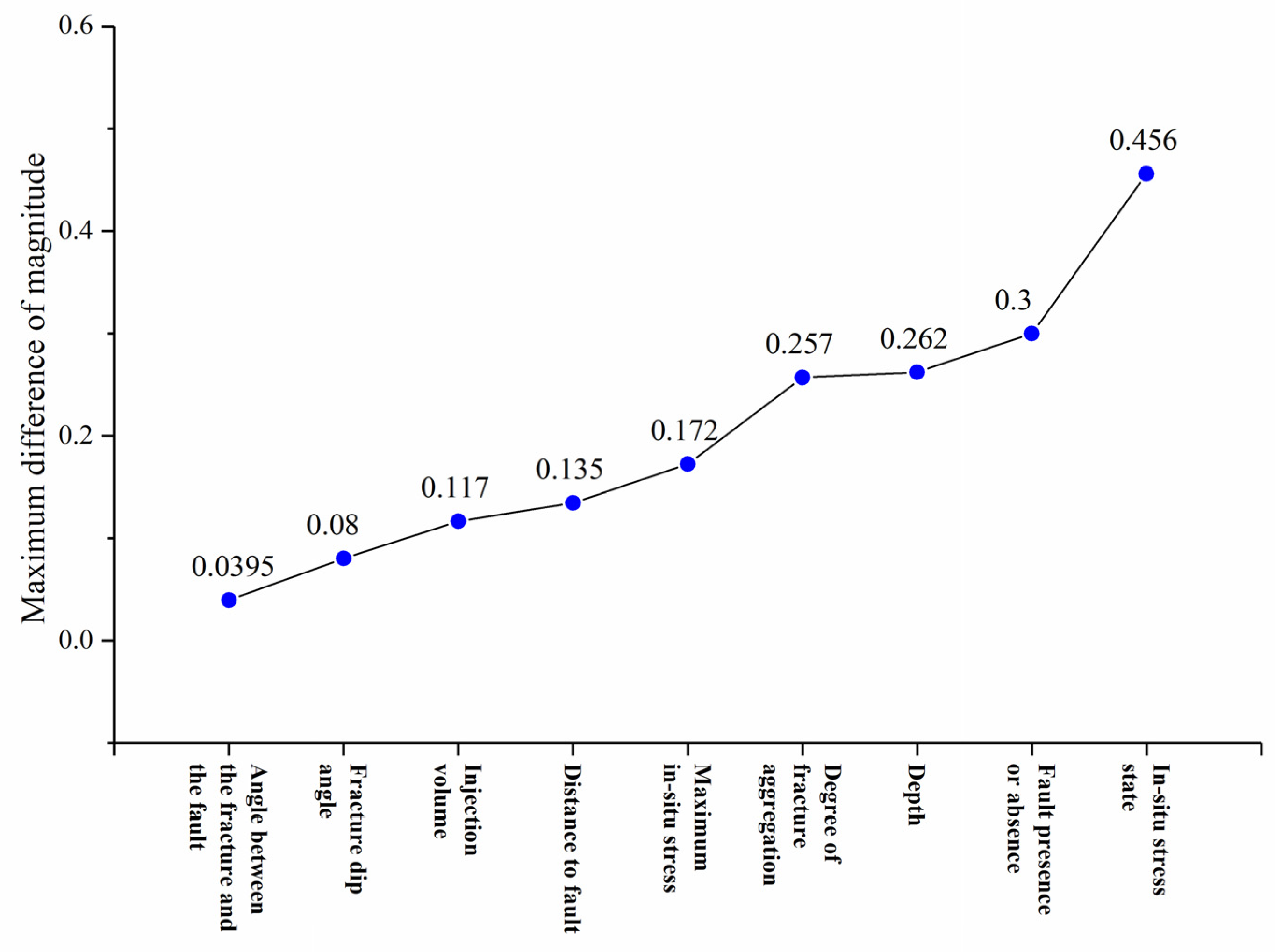
3. Parameter Sensitivity Analysis

The trained neural network model can be used to induce seismicity evaluation. As shown in Table 1, among the nine input parameters, each item is divided into several different situations. If all the situations are traversed, a total of 180,000 situations need to be calculated, which is too much of a calculation. Therefore, we divide the nine parameters into two groups, excluding the fault presence or absence. The first group of parameters includes in situ stress state, fracture dip angle, maximum in situ stress and depth. The second group of parameters includes injection volume, the angle between the fracture and the fault, the degree of fracture aggregation and the distance to fault. Dividing these input parameters into two groups and analyzing the influence of each group of input parameters on inducing seismicity, respectively, can greatly reduce the amount of calculation [27,28,29].

In the absence of fault, we can analyze the influence of maximum in situ stress, depth, in situ stress state, and fracture dip angle on inducing seismicity. Figure 6 shows the variation in the magnitude of the induced seismicity with the maximum in situ stress and depth obtained from the neural network model. Figure 6a shows the result of the induced seismicity without fault, and Figure 6b shows the result of the induced seismicity with fault. As shown in the figure, under the combined effect of the maximum in situ stress and depth factor, a smaller maximum in situ stress and a larger depth will result in a smaller seismicity magnitude. In the absence of fault, the maximum seismicity magnitude difference caused by the maximum in situ stress is 0.1723, and the maximum seismicity magnitude difference caused by depth is 0.2552. In the case of fault, the maximum seismicity magnitude difference caused by the maximum in situ stress is 0.1705, and the maximum seismicity magnitude difference caused by depth is 0.2621. It can be known through comparison that the maximum magnitude in the case of fault is greater than that in the case without fault, and the maximum magnitude difference is 0.3. Among the combined factors of maximum in situ stress and depth, the maximum in situ stress plays a dominant role.

Figure 7 shows the variation in the induced seismicity magnitude with in situ stress state and fracture dip angle obtained from the neural network model. In Figure 7, (a) shows the induced seismicity results without fault, and (b) shows the induced seismicity results with fault. As shown in the figure, under the combined factor of in situ stress state and fracture dip angle, a smaller seismicity magnitude is generated under the normal faulting stress state, while the seismicity magnitude generated under the reverse faulting stress state is larger. However, the fracture dip angle has a small and insignificant influence on the seismicity magnitude. In the absence of fault, the maximum seismicity magnitude difference caused by the in situ stress state is 0.373, and the maximum seismicity magnitude difference caused by the fracture dip angle is 0.035. In the case of fault, the maximum seismicity magnitude difference caused by the in situ stress state is 0.456, and the maximum seismicity magnitude difference caused by the fracture dip angle is 0.08. It can be revealed through comparison that the maximum magnitude in the case of fault is greater than that in the case without fault, and the maximum magnitude difference is 0.2842. Among the combined factors of in situ stress state and fracture dip angle, the in situ stress state plays a dominant role.

For the second set of input control parameters—injection volume, fracture-fault angle, the degree of fracture aggregation, and distance to the fault—the influence patterns are shown in Figure 8a. This sub-figure particularly focuses on how the fracture-fault angle and the degree of fracture aggregation jointly affect the intensity of induced seismicity. The analysis results indicate that the more dispersed the fracture network, the smaller the intensity of seismic activity.

However, the angle between the fracture and the fault has no obvious influence on the magnitude of the seismicity. Among them, the maximum seismicity magnitude difference caused by the degree of fracture aggregation is 0.257, while the maximum seismicity magnitude difference caused by the angle between the fracture and the fault is 0.0395. Among the combined factors of the angle between fractures and fault and the degree of fracture aggregation, the degree of fracture aggregation plays a leading role. In Figure 8, (b) shows the variation in the induced seismicity magnitude with the injection volume and the distance to fault. Under the combined factor of injection volume and distance to fault, a smaller injection volume and a larger distance to fault will lead to a reduction in the magnitude of the seismicity. Among them, the maximum seismicity magnitude difference caused by the injection volume is 0.1167, and the maximum seismicity magnitude difference caused by the distance to fault is 0.1347. Therefore, among the combined factors of injection volume and distance to fault, the effect of distance to fault is slightly greater than that of injection volume.

To minimize the harm caused by induced seismicity as much as possible, it is necessary to control the magnitude of induced seismicity. Based on the above analysis, the nine input parameters are sorted according to the maximum magnitude differences caused by each input parameter to represent the degree of influence of each parameter on the seismicity magnitude. Among them, the in situ stress state has the greatest influence on the magnitude of seismicity, even greater than that of fault on seismicity. However, the occurrence of fractures (including the fracture dip angle and the angle between fractures and fault) has a relatively small influence on the magnitude of seismicity. To sum up, in order of the influence degree of each parameter on the magnitude of a seismicity, from largest to smallest, they are as follows: in situ stress state, fault presence or absence, depth, degree of fracture aggregation, maximum in situ stress, distance to fault, injection volume, fracture dip angle, and the angle between the fracture, and the fault, as shown in Figure 9.

In order to reduce the magnitude of induced seismicity, it is necessary to avoid factors that have a significant impact on the magnitude of seismicity as much as possible in actual engineering operations. For example, in the site selection process, fault should be avoided as much as possible or the distance to fault should be too far. In terms of in situ stress state, areas with normal faulting stress state or strike-slip faulting stress state should be selected as much as possible, and areas with reverse faulting stress state should be avoided. At the same time, it is necessary to avoid excessive seismicity magnitude caused by excessive in situ stress as much as possible. In addition, areas with well-developed and relatively scattered fractures should be selected as much as possible, and the drilling depth should also be ensured to be sufficiently deep, so as to ensure that the magnitude of the seismicity can be controlled within a certain range. As for the occurrence of fractures, their influence on the magnitude of seismicity is relatively small. A little attention should be paid during the site selection of geothermal projects and geological surveys. Since the injection volume during the fracturing process is controllable by humans, in actual engineering, the injection volume needs to be controlled in combination with the actual situation on site. In conclusion, the EGS project should be located in areas with normal faulting stress state or strike-slip faulting stress state and relatively low in situ stress as much as possible. Moreover, it is necessary to avoid fault or areas that are either too close to faults, located at deep depth, or characterized by dispersed fractures as much as possible, in order to reduce the magnitude of induced seismicity and avoid the hazards caused by induced seismicity.

During the calculation process of the neural network model, each input parameter is assigned a certain weight before participating in the calculation, as shown in Equation (2). The initial weight value of each input parameter is set to 1. After the model is trained, it still needs to be analyzed based on the calculation results and then the initial weights need to be corrected. Sort the parameters according to the degree of influence of each parameter on the seismicity magnitude and then assign weights to each parameter based on its importance. Assume the total weight value is 1. The corrected weights are shown in

Table 3. The corrected weight values of each parameter.

Parameters	Ranking of the Degree of Influence	The Corrected Weight Value
In situ stress state	1	0.2
Fault presence or absence	2	0.18
Depth	3	0.16
Degree of fracture aggregation	4	0.13
Maximum in situ stress	5	0.11
Distance to fault	6	0.09
Fluid injection volume	7	0.07
Fracture dip angle	8	0.04
The angle between fracture and fault	9	0.02

. Applying the optimized parameter weights to Equation (2) and correcting the model parameters can, to a certain extent, improve the computational accuracy and operational efficiency of the neural network.

By conducting sensitivity analysis on each input parameter in the neural network model, the weights of each input parameter can be corrected according to the influence degree of the seismicity magnitude. The revised weight values are directly integrated into the neural network model, which helps to improve its calculation accuracy. More importantly, by analyzing the specific influence patterns of different parameters on the intensity of induced seismic activities, this model can provide important references and risk assessment basis for key links such as the site selection evaluation, geological exploration of the enhanced geothermal system (EGS) project, and the design of reservoir stimulation (fracturing, etc.) schemes. Based on this, targeted measures can be formulated to effectively reduce or avoid the potential engineering risks and environmental hazards caused by induced seismic events.

4. Model Application

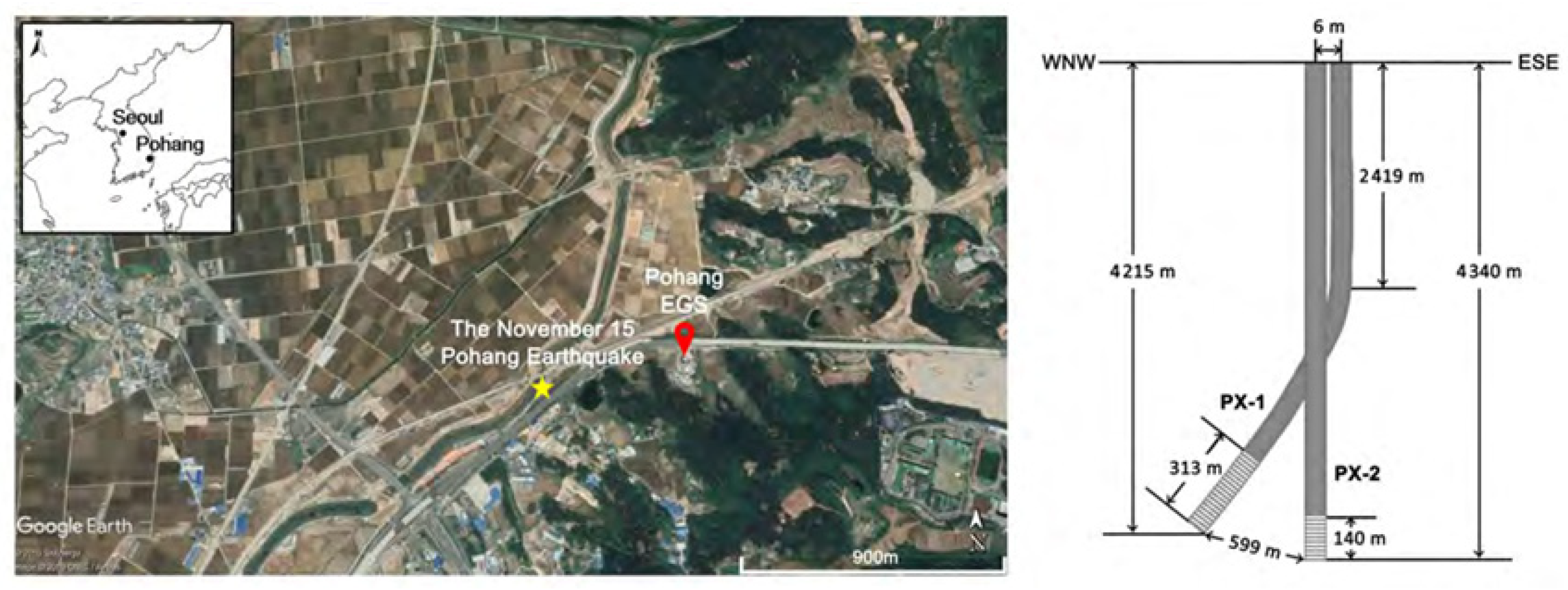
4.1. Pohang EGS Project Overview

On 15 November 2017, a seismicity occurred in Pohang, South Korea, with a magnitude as high as 5.5. According to the estimation of relevant departments in South Korea, the seismicity injured 135 residents, urgently evacuated over 1700 people, caused direct losses of more than 75 million dollars, and had a total economic impact of more than 300 million dollars. This is the most destructive seismicity that has occurred on the Korean Peninsula in several centuries. The drilling site of South Korea’s first enhanced geothermal system (EGS) project is near the epicenter (Figure 10). At present, international scholars generally believe that the injection fluid of the Pohang EGS project caused fault sliding, thereby inducing a magnitude 5.4 seismicity [30].

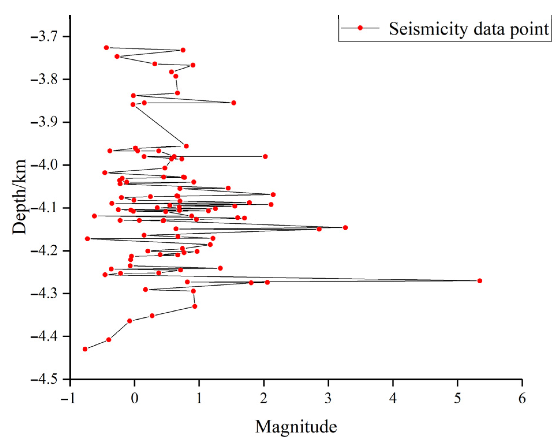
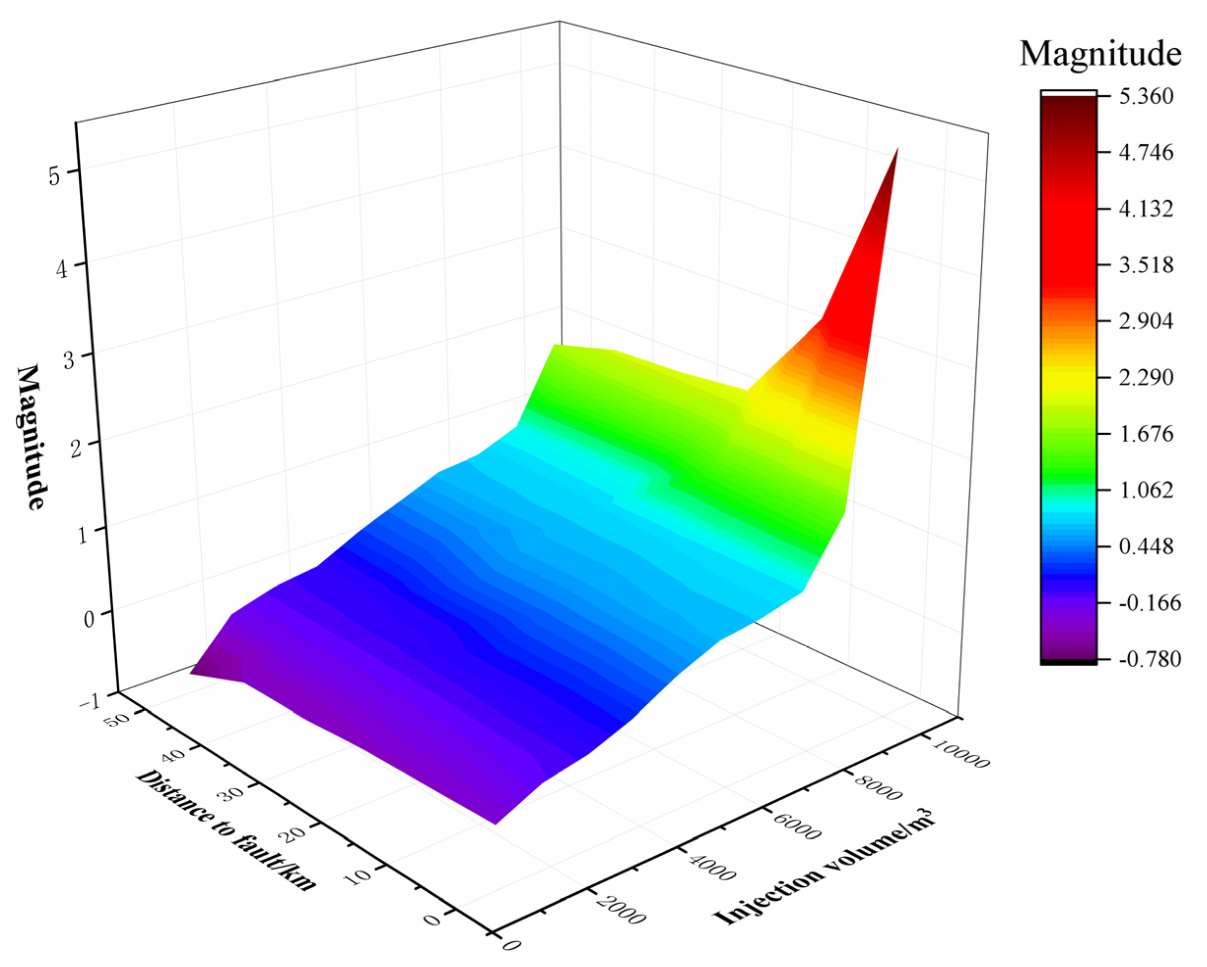
4.2. Application of Neural Network Model

Based on the artificial neural network (ANN) model established by us earlier, it was applied to the Pohang EGS site in South Korea for the assessment of induced seismicity. Then, the assessment results were compared with the actual site-induced seismicity situation to test the accuracy of the model calculation results, and the model was corrected based on the comparison between the predicted results and the actual results to better reflect the actual conditions. Although the model has been trained to a certain extent before, it is still necessary to substitute the seismic data information and related engineering parameters of the study area into the network model for secondary training, so as to make the model more in line with the actual situation of the study area.

Although a large amount of seismicity data information can make the results more accurate, since South Korea began national seismicity monitoring in 1978, only 15 seismicity with Ms ≥ 2.5 have been recorded, and among them, only 11 records have detailed data that can be used for seismicity analysis. Therefore, based on these 11 sets of data, combined with the data of seven induced seismicity that have occurred in typical geothermal development zones around the world [5,31,32], as well as some of the seismicity data generated during the actual development process of the Pohang EGS project (98 sets), we integrated these 116 sets of data and substitute them into the artificial neural network model for training and correction of the model. Subsequently, based on the actual conditions of the study area (Pohang geothermal field), a comprehensive assessment of the induced seismic activity was conducted.

The detailed seismic activity parameters used for the assessment are listed in

Table 4. Data of natural seismicity (Ms ≥ 2.5) near Pohang and some typical induced seismicity.

	Fluid Injection Volume	Distance to Fault	Depth	In Situ Stress		Maximum Magnitude	Focal Mechanism
				Magnitude	Direction
1	0	66 km	10 km	158 MPa	244°	3.5	Unknown
2	0	172 km	5.4 km	86 MPa	22°	4.7	Sinistral reverse
3	0	168 km	10 km	129 MPa	101°	4.7	Unknown
4	0	172 km	11.5 km	182 MPa	26°	5.5	Dextral reverse
5	0	137 km	10 km	113 MPa	119°	3.5	Unknown
6	0	57 km	8.8 km	139 MPa	73°	4.6	Dextral normal
7	0	59.8 km	13 km	206 MPa	29°	5.4	Dextral Strike-slip
8	0	54.9 km	10 km	129 MPa	49°	4.9	Unknown
9	0	56 km	10 km	113 MPa	214°	4.7	Unknown
10	0	25 km	10 km	158 MPa	225°	4.8	Unknown
11	0	161 km	10 km	129 MPa	43°	4.4	Sinistral normal
12	9 × 102 m3	0.21 km	5.49 km	243 MPa	75°	5.5	Reverse
13	2 × 104 m3	0.34 km	4.13 km	91 MPa	101°	3.7	Unknown
14	4 × 104 m3	1.21 km	4.98 km	91.3 MPa	175°	2.9	Unknown
15	2 × 108 m3	0.58 km	2.5 km	72.3 MPa	155°	4.4	Dextral
16	1.1566 × 104 m3	1.35 km	5 km	115 MPa	144°	3.4	Unknown
17	1.36 × 1010 m3	6 km	3.39 km	98.3 MPa	26°	4.6	Dextral normal
18	4 × 103 m3	0.47 km	9.1 km	150 MPa	166°	1.2	Unknown

. This table integrates 18 seismic events, including 11 earthquakes that occurred within the study area with a magnitude of 2.5 or greater, and seven typical induced seismic events triggered by global typical geothermal development projects. To improve the accuracy of the model predictions, necessary data preprocessing was carried out before inputting the seismic activity parameters into the model. Finally, a trained neural network model was applied to quantitatively assess the specific seismic activity induced by fluid injection at the Pohang Enhanced Geothermal System (EGS) site. The assessment results and analyses are visually presented in Figure 11 and Figure 12.

In the established model, the drilling depth of the Pohang EGS site is 3.7 km, the maximum in situ stress is 243 MPa, and the direction of the maximum in situ stress is 77°. Firstly, we studied the variation in the magnitude of the induced seismicity with depth. With the increase in depth, the magnitude of seismicity also showed a gradually increasing trend, as shown in Figure 11. Since the drilling depth is 3.7 km, the induced seismicity generated are all below 3.7 km and reach a depth close to 4.5 km. Most of the seismicity generated in this simulation had magnitudes less than 1. There were a total of 19 seismic events with magnitudes greater than 1 and 7 seismicity with magnitudes greater than 2. Among them, the magnitude of the largest seismicity event was 5.34, which was close to the magnitude 5.5 seismicity that occurred in the actual Pohang project. Overall, with the increase in depth, the magnitudes of most seismic events are still concentrated between −1 and 2, but larger magnitude events (>1 magnitude) will increase with the increase in depth. Seismicity of magnitude 2.0 or above began to occur when the depth was greater than 4 km. The largest seismicity of magnitude 5.34 occurred at a distance of 4.27 km. Therefore, we can conclude that an increase in depth will lead to a rise in the magnitude of seismic events, and most seismicity with larger magnitudes occur at greater depths.

Figure 12 shows the trend of seismicity magnitude variation with injection volume and distance to fault. It can be seen from the figure that with the increase in the injection volume and the decrease in the distance to fault, the seismicity magnitude shows a gradually increasing trend. Among them, the increase in the injected volume caused a very obvious increase in the magnitude of the seismicity. When the injected volume approached 10,000 m³, a seismicity event of magnitude 5.34 occurred. There is a sudden change in the magnitude of seismicity in this part. The reason might be that the injection volume is too large, causing the injected energy to exceed the maximum energy that the underground structure can withstand, resulting in the destruction of the underground structure, the sliding of the fault, and thus leading to the occurrence of a large seismicity. This is also consistent with the fact that there is fault in the lower part of the Pohang EGS site, verifying the accuracy of our model from the side. However, the increase in distance to fault does not have a very obvious impact on the magnitude of seismicity. With the increase in the distance to fault, the magnitude of seismicity also shows a gradually increasing trend, but the change is not very obvious. The sudden change in the magnitude of seismicity events also occurs in areas with smaller distance to fault, which also proves from another aspect the influence of distance to fault on seismicity events.

5. Discussion

Neural network applications in the evaluation assessment of geothermal-induced seismicity have recently crystallized into several core research directions [33,34,35]. In the aspects of seismic activity prediction and risk assessment, researchers utilize Long Short-Term Memory networks (LSTM) and gated recurrent units (GRU) to analyze time series data, such as injection pressure, flow rate, and historical earthquake catalogs, in order to capture the delayed response relationship between fluid injection and earthquake activity [13,36,37]. For instance, Liang et al. [38] processed the hydraulic stimulation and tracer tests using numerical models and LSTM neural network models and applied them to the Habinore geothermal system in Australia, significantly improving the prediction accuracy of injection wellhead pressure and tracer agent concentration output. Meanwhile, Convolutional Neural Networks (CNN) are used to process spatially grid-based data, such as Shaheen et al. [39], who proposed a convolutional neural network (CNN) to detect seismic events from the shallow borehole stations in Groningen, the Netherlands. The proposal of this method facilitates its application and promotion to other microseismic monitoring networks that incorporate multiple sensors. At the same time, researchers such as Grigoli used artificial neural networks to predict and evaluate the probability of possible future seismic activities and the magnitude range in the Geysers geothermal field in the United States [14]. Deichmann et al. used the ANN model to predict the spatiotemporal evolution of seismic activities in the Basel geothermal project in Switzerland [15]. Gaucher et al. et al. effectively used the ANN model to predict the spatiotemporal evolution of seismic activities in the Icelandic geothermal field and identified high-risk areas [16].

In this study, the internal structure of the artificial neural network was improved. To ensure that the initial input values of each neuron are as close as possible to the origin of the coordinate axis, two methods were combined. Firstly, the initial weights of the neurons were made as small as possible, while ensuring that the number of initial weights with positive and negative values was equal. After conducting a sensitivity analysis, the weights of each parameter were corrected, significantly improving the accuracy of the model. Compared with the results of other researchers [40], through the model analysis results, the different degrees of influence of different geological parameters and artificial operation parameters on inducing seismic activities were obtained. Thus, in the actual geothermal development process, according to the different degrees of influence, relevant parameters can be artificially controlled to reduce or avoid the occurrence of induced seismic activities, thereby ensuring the safe operation of the EGS project.

This paper also expands the data set through data augmentation techniques to enhance the generalization ability of the model. In the results of other researchers, the scarcity of data severely restricts the generalization ability of the model, especially the problem of insufficient samples for inducing major seismic activities (M > 3) is particularly prominent. By introducing data augmentation techniques, the problem of insufficient data can be significantly alleviated, the generalization ability of the model can be improved, and thus the accuracy of the model can be enhanced.

Finally, this model was applied to the Pohang EGS project, and the causes of the 5.4 magnitude earthquake were analyzed. The black-box output results of the neural network model were combined with the actual physical process, shifting the purely data-driven model towards a physical-constrained architecture to ensure physical consistency. Under the premise of not violating the mechanical principles, the prediction and evaluation of EGS-induced seismic activities were conducted through the neural network model.

In summary, in response to the induced seismicity issue during the EGS engineering development process, we have established an induced seismicity evaluation model based on artificial neural networks. We introduced data augmentation techniques to alleviate the problem of insufficient data and enhance the model’s generalization ability. Then, we improved the model’s accuracy through weight correction. Finally, we combined the data-driven approach of the model with physical constraints to ensure physical consistency. This model can be used for the induced seismic evaluation of future EGS projects and provide a reference for project site selection and induced seismic risk warning.

6. Conclusions

Based on the artificial neural network model, this study selected nine influencing factors that induce seismicity as the neuron input parameters, conducted sensitivity analysis and weight correction on these parameters, and finally established the evaluation model of induced seismicity. Then it was applied to the Pohang EGS project in South Korea, and the analysis and evaluation of the influencing factors of induced seismicity were carried out. The following conclusions were drawn below:

(1) Nine parameters were selected as the input parameters of the induced seismicity evaluation model. The influence degrees of each parameter on the magnitude of the induced seismicity, from large to small, are as follows: in situ stress state, presence or absence of fault, depth, degree of fracture aggregation, maximum in situ stress, distance to fault, injection volume, fracture dip angle, and the angle between the fracture and the fault.

(2) The induced seismicity evaluation model was applied to analyze and evaluate the influencing factors of induced seismicity in the Pohang EGS site. It was estimated that the induced seismicity generated were all below 3.7 km (drilling depth). With the increase in depth, the seismicity magnitude also showed a gradually increasing trend. Higher injection volumes and closer fault distances both result in greater seismicity magnitude.

(3) The evaluation results of the Pohang EGS engineering model show that when the injection volume is close to 10,000 m³, the magnitude of the seismicity increases sharply, and the maximum magnitude reaches 5.34. This might be because the injected energy exceeds the maximum energy that the underground structure can bear, causing the underground structure to be damaged, fault to slide, and thus leading to the occurrence of major seismicity.

References

1. Ellabban, H.; Abu-Rub, F. Blaabjerg. Renewable energy resources: Current status, future prospects and their enabling technology. Renew. Sustain. Energy Rev. 2014, 39, 748–764. [Google Scholar] [CrossRef]
2. Barbier, E. Geothermal Energy Technology and Current Status: An Overview. Renew. Sustain. Energy Rev. 2002, 6, 3–65. [Google Scholar] [CrossRef]
3. Olasolo, P.; Juárez, M.C.; Morales, M.P.; Damico, S.; Liarte, I.A. Enhanced geothermal systems (EGS): A review. Renew. Sustain. Energy Rev. 2016, 56, 133–144. [Google Scholar] [CrossRef]
4. Lu, S.-M. A global review of enhanced geothermal system (EGS) Renew. Sustain. Energy Rev. 2018, 81, 2902–2921. [Google Scholar] [CrossRef]
5. Majer, E.L.; Baria, R.; Stark, M.; Oates, S.; Bommer, J.; Smith, B.; Asanuma, H. Induced seismicity associated with Enhanced Geothermal Systems. Geothermics 2007, 36, 185–222. [Google Scholar] [CrossRef]
6. Catalli, F.; Rinaldi, A.P.; Gischig, V.; Nespoli, M.; Wiemer, S. The importance of earthquake interactions for injection-induced seismicity: Retrospective modeling of the Basel Enhanced Geothermal System. Geophys. Res. Lett. 2016, 43, 4992–4999. [Google Scholar] [CrossRef]
7. Goertz-Allmann, B.; Goertz, A.; Wiemer, S. Stress Drop Variations of Induced Earthquakes at the Basel Geothermal Site. Geophys. Res. Lett. 2011, 38, L09308. [Google Scholar] [CrossRef]
8. Johnson, L.R.; Majer, E.L. Induced and triggered earthquakes at The Geysers geothermal reservoir. Geophys. J. Int. 2017, 209, 1221–1238. [Google Scholar] [CrossRef]
9. Lin, G.; Thurber, C.H. Seismic velocity variations along the rupture zone of the 1989 Loma Prieta earthquake, California. J. Geophys. Res. 2012, 117. [Google Scholar] [CrossRef]
10. Kim, K.-H.; Ree, J.-H.; Kim, Y.; Kim, S.; Su, Y.K.; Seo, W. Assessing whether the 2017 Mw 5.4 Pohang earthquake in South Korea was an induced event. Science 2018, 360, 6392. [Google Scholar] [CrossRef]
11. Shapiro, S.A.; Kim, K.H.; Ree, J.H. Magnitude and nucleation time of the 2017 Pohang Earthquake point to its predictable artificial triggering. Nat. Commun. 2021, 12, 6397. [Google Scholar] [CrossRef] [PubMed]
12. Shan, K.; Zhang, Y.; Zheng, Y.; Li, L.; Deng, H. Risk assessment of fracturing induced earthquake in the Qiabuqia Geothermal Field, China. Energies 2020, 13, 5977. [Google Scholar] [CrossRef]
13. Prezioso, E.; Sharma, N.; Piccialli, F.; Convertito, V. A data-driven artificial neural network model for the prediction of ground motion from induced seismicity: The case of the geysers geothermal field. Front. Earth Sci. 2022, 10, 917608. [Google Scholar] [CrossRef]
14. Grigoli, F.; Cesca, S.; Priolo, E.; Rinaldi, A.P.; Clinton, J.F.; Stabile, T.A.; Dost, B.; Fernandez, M.G.; Wiemer, S.; Dahm, T. Current challenges in monitoring, discrimination, and management of induced seismicity related to underground industrial activities: A European perspective. Rev. Geophys. 2017, 55, 310–340. [Google Scholar] [CrossRef]
15. Deichmann, N.; Giardini, D. Earthquakes induced by the stimulation of an enhanced geothermal system below basel (Switzerland). Seismol. Res. Lett. 2020, 80, 784–798. [Google Scholar] [CrossRef]
16. Gaucher, E.; Schoenball, M.; Heidbach, O.; Zang, A.; Fokker, P.A.; van Wees, J.D.; Kohl, T. Induced seismicity in geothermal reservoirs: A review of forecasting approaches. Renew. Sustain. Energy Rev. 2015, 52, 1473–1490. [Google Scholar] [CrossRef]
17. Schmidhuber, J. Deep learning in neural networks: An overview. Neural Netw. 2015, 61, 85–117. [Google Scholar] [CrossRef]
18. Jordan, M.I.; Mitchell, T.M. Machine learning: Trends, perspectives, and prospects. Science 2015, 349, 255–260. [Google Scholar] [CrossRef]
19. Adeli, H.; Panakkat, A. A probabilistic neuralnetwork for earthquake magnitude prediction. Neural Netw. 2009, 22, 1018–1024. [Google Scholar] [CrossRef] [PubMed]
20. Wang, Q.; Guo, Y.; Yu, L.; Li, P. Earthquake prediction based on spatio-temporal data mining: An LSTM network approach. IEEE Trans. Emerg. Top. Comput. 2017, 8, 148–158. [Google Scholar] [CrossRef]
21. Ashif, P.; Hojjat, A. Neural network model for earthquake magnitude prediction using multiple seismicity indicator. Int. J. Syst. 2007, 17, 13–33. [Google Scholar]
22. Panakkat, A.; Adeli, H. Recurrent neural network for approximate earthquake time and location prediction using multiple seismicity indicators. Comput. Aided Civ. Infrastruct. Eng. 2009, 24, 280–292. [Google Scholar] [CrossRef]
23. Zhang, H.; Alkhalifah, T.; Liu, Y.; Birnie, C.; Di, X. Improving the generalization of deep neural networks in seismic resolution enhancement. IEEE Geosci. Remote Sens. Lett. 2023, 20, 1–5. [Google Scholar] [CrossRef]
24. Zhou, J.C.; Wen, X.Y.; Guo, M.J. A symmetric difference data enhancement physics-informed neural network for the solving of discrete nonlinear lattice equations. Commun. Theor. Phys. 2025, 77, 065002. [Google Scholar] [CrossRef]
25. Yu, X.; Jin, G.; Li, J. Target tracking algorithm for system with gaussian/non-gaussian multiplicative noise. IEEE Trans. Veh. Technol. 2019, 69, 90–100. [Google Scholar] [CrossRef]
26. Kotecha, J.H.; Djuric, P.M. Gaussian particle filtering. IEEE Trans. Signal Process. 2003, 51, 2592–2601. [Google Scholar] [CrossRef]
27. Drechsler, M. Sensitivity analysis of complex models. Biol. Conserv. 1998, 86, 401–412. [Google Scholar] [CrossRef]
28. Liu, Y.P.; Wang, S.; Gong, C.S.; Zeng, D.W.; Ren, Y.L.; Li, X. Sensitivity Analysis of the Land Surface Characteristic Parameters in Different Climatic Regions of the Loess Plateau. Atmosphere 2023, 14, 1528. [Google Scholar] [CrossRef]
29. Xue, X.; Ren, Z.Y.; Zhang, Y.X.; Gao, A.H. The study of sensitivity analysis of parameters of groundwater numerical simulation. Adv. Mat. Res. 2013, 726, 3564–3569. [Google Scholar] [CrossRef]
30. Li, Z.; Elsworth, D.; Wang, C. Constraining maximum event magnitude during injection-triggered seismicity. Nat. Commun. 2021, 12, 1528. [Google Scholar] [CrossRef]
31. Grünthal, G. Induced seismicity related to geothermal projects versus natural tectonic earthquakes and other types of induced seismic events in central Europe. Geothermics 2014, 52, 2235. [Google Scholar] [CrossRef]
32. Yeo, I.-W.; Brown, M.R.M.; Ge, S.; Lee, K.K. Causal mechanism of injection-induced earthquakes through the Mw 5.5 Pohang earthquake case study. Nat. Commun. 2020, 11, 2614. [Google Scholar] [CrossRef]
33. Zheng, Y.; Li, J.; Zhu, T.; Li, J. Experimental and MPM modelling of widened levee failure under the combined effect of heavy rainfall and high riverine water levels. Comput. Geotech. 2025, 184, 107259. [Google Scholar] [CrossRef]
34. Picozzi, M.; Iaccarino, A.G. Forecasting the preparatory phase of induced earthquakes by recurrent neural network. Forecasting 2021, 3, 17–36. [Google Scholar] [CrossRef]
35. Nooshiri, N.; Bean, C.J.; Dahm, T.; Grigoli, F.; Kristjansdottir, S.; Obermann, A.; Wiemer, S. A multi-branch, multi-target neural network for rapid point-source inversion in a micro-seismic environment: Examples from the hengill geothermal field, iceland. Geophys. J. Int. 2022, 229, 999–1016. [Google Scholar] [CrossRef]
36. Zheng, Y.; Coop, M.R.; Tang, H.; Fan, Z. Effects of overconsolidation on the reactivated residual strength of remoulded deep-seated sliding zone soil in the Three Gorges Reservoir Region, China. Eng. Geol. 2022, 310, 106882. [Google Scholar] [CrossRef]
37. Yang, Y.X.; Zhang, Y.; Cheng, Y.; Lei, Z.; Gao, X.; Huang, Y.; Ma, Y. Using one-dimensional convolutional neural networks and data augmentation to predict thermal production in geothermal fields. J. Clean. Prod. 2023, 387, 135879. [Google Scholar] [CrossRef]
38. Liang, X.; Xu, T.; Chen, J.; Jiang, Z. A deep-learning based model for fracture network characterization constrained by induced micro-seismicity and tracer test data in enhanced geothermal system. Renew. Energy 2023, 216, 119046. [Google Scholar] [CrossRef]
39. Shaheen, A.; Waheed, U.B.; Fehler, M.; Sokol, L.; Hanafy, S. GroningenNet: Deep learning for low-magnitude earthquake detection on a multi-level sensor network. Sensors 2021, 21, 8080. [Google Scholar] [CrossRef]
40. Yin, X.X.; Jiang, C.S.; Yin, F.L.; Zhai, H.Y.; Zheng, Y.; Wu, H.D.; Niu, X.; Zhang, Y.; Jiang, C.; Li, J.W. Assessment and optimization of maximum magnitude forecasting models for induced seismicity in enhanced geothermal systems: The Gonghe EGS Project in Qinghai, China. Tectonophysics 2024, 886, 230438. [Google Scholar] [CrossRef]
Figure 1. Different degrees of fracture aggregation: (1) The fractures are evenly distributed; (2) The fractures began to converge towards the fault; (3) The fractures further converge towards the fault; (4) The fractures are concentrated near the fault.
Energies 18 04004 g001
Figure 2. Schematic diagram of the neural network structure.
Energies 18 04004 g002
Figure 3. Schematic of the established 3D geothermal reservoir model.
Energies 18 04004 g003
Figure 4. Comparison of numerical simulation results and model training results: (a) The comparison between the maximum magnitude results obtained from the numerical simulation of the training dataset and those from the model training process; (b) The comparison between the quantity of seismicity results obtained from the numerical simulation of the training dataset and those from the model training process; (c) The comparison between the seismicity distance results obtained from the numerical simulation of the training dataset and those from the model training process; (d) The relative error between the numerical simulation results and the model training results.
Energies 18 04004 g004
Figure 5. Accuracy verification of the data set: (a) The data fitting results of the training group. (b) The data fitting results of the verification group. (c) The data fitting results of the test group. (d) The data fitting results of all data.
Energies 18 04004 g005
Figure 6. Variation in induced seismicity magnitude with the maximum in situ stress and depth.
Energies 18 04004 g006
Figure 7. Variation in induced seismicity magnitude with in situ stress state and fracture dip angle.
Energies 18 04004 g007
Figure 8. Variation in induced seismicity magnitude with the angle between the fracture and the fault and the degree of fracture aggregation (a), as well as with the injection volume and the distance to fault (b).
Energies 18 04004 g008
Figure 9. Maximum magnitude difference under the influence of various parameters.
Energies 18 04004 g009
Figure 10. Schematic diagram of the Pohang EGS project.
Energies 18 04004 g010
Figure 11. Variation in seismicity magnitude with depth.
Energies 18 04004 g011
Figure 12. The variation in induced seismicity magnitude with fault distance and injection volume.
Energies 18 04004 g012