Integrating BIM Forward Design with CFD Numerical Simulation for Wind Turbine Blade Analysis

Abstract

Wind turbine blades face significant challenges from stochastic wind loads, impacting structural integrity. Traditional analysis often isolates Computational Fluid Dynamics (CFD) from Building Information Modeling (BIM) in the design process. This study bridges this gap by integrating BIM forward design with CFD simulation. A universal BIM modeling framework is developed for rapid blade modeling, which is compatible with ANSYS Workbench 2022 R1 through intermediate format conversion. The influence of wind load on the blades under various wind speed conditions is analyzed, and the results indicate a significant correlation between wind load intensity and blade structural response. The maximum windward pressure reaches 4.96 kPa, while the leeward suction peaks at −6.28 kPa. The displacement at the tip and middle part of the blades significantly increases with the increase in wind speed. The growth rate of displacement between adjacent speeds rises from 1.20 to 1.94, and the overall increase rate within the entire range rises from 1.02 to 4.16. These results demonstrate the feasibility of using BIM forward design in accurate performance analysis, and also extends the value of BIM in wind energy. Furthermore, a bidirectional information flow is established, where BIM provides geometry for CFD, and simulation results will inform BIM design refinement.

1. Introduction

With the increasing global concern about and demand for renewable energy, wind energy, as a clean and sustainable form of power, has been widely promoted and adopted worldwide [1]. The wind turbine is the essential piece of equipment for converting wind energy into electricity. In recent years, it has been continuously developed to be larger and lighter [2]. The length of its blades is increasing, while its structural safety margin is decreasing. Especially for long, flexible blades, structural damage or failure may occur during operation [3]. Wind load, due to its unpredictability, dynamic changes and destructive potential, is the primary cause of blade breakage, fracture and even complete structural failure. It is also an important factor to be considered in design [4]. Therefore, to ensure that a blade design can withstand complex wind load conditions, conducting an initial analysis of its rationality is crucial. This requires us to explore an efficient and accurate design analysis method.

Wind turbine blades have the characteristics of high unit cost and complex multidisciplinary coupling design [5], and traditional trial-and-error development faces huge economic risks. Therefore, high-fidelity models are needed to improve analysis accuracy in order to more accurately reflect the real performance of blades under the action of the flow field and reduce the cost of trial and error and the risk of operation and maintenance. ANSYS is a widely used simulation analysis software that provides a comprehensive and integrated simulation solution covering the entire process from 3D model construction to performance analysis, and it is applied in various engineering fields, including structural [6], fluid [7], heat transfer [8] and electromagnetic [9]. DesignModeler (DM), as the built-in modeling software in ANSYS, has excellent solid modeling capabilities [10]. However, it has certain limitations when dealing with complex geometric shapes and structural features, especially when constructing wind turbine blades with complex, variable cross-sections and twisted shapes, which demand more time and effort [11]. Meanwhile, although the current design process can quickly achieve the digitalization of design results, its essence of “drawing first, then modeling” perpetuates the information fragmentation in the workflow [12], resulting in 30% to 50% of design changes occurring during the model reconstruction process in the construction stage [13]. Such late-stage modifications inevitably lead to cost overruns and project delays [14], which exposes the critical need for a paradigm shift in engineering workflows.

Building Information Modeling (BIM) [15] establishes a data-centric paradigm by integrating parametric modeling, multidisciplinary collaboration and real-time information sharing [16] from the conceptual phase onward. This method constructs a digitally integrated twin [17] that encapsulates the geometric, semantic and behavioral attributes of building components, ensuring data continuity throughout the entire design–construction life cycle [18]. BIM has become a key strategy for addressing the inherent limitations of traditional fragmented workflows [19], not only eliminating information silos but also enabling predictive simulations during the design phase [17], thereby fundamentally preventing the need for reactive changes in later stages. Meanwhile, BIM platforms typically offer a high degree of data interoperability, which enables easy data exchange and integration with other software [20]. This enables the blade simulation model construction process to easily access externally imported model parameters for refined model construction. In contrast, DM, the built-in software in ANSYS, focuses more on numerical analysis and simulation calculations [21] and is much less specialized and flexible than BIM technology in model construction. Therefore, this study applies BIM technology during the model construction phase to create models of wind turbine blades and explores the application of BIM in forward design.

The analysis of aerodynamic performance under wind load is crucial for the design of wind turbine blades. In addition to the accuracy of model construction, selecting an appropriate performance analysis method is essential. Common methods for analyzing the aerodynamic performance of wind turbine blades include field tests, wind tunnel tests, numerical simulations and theoretical calculations. Field tests and wind tunnel tests require high-precision equipment and specialized technology support, which can lead to relatively high costs. The theoretical calculation method is usually applicable to some specific working-condition parameters. For some complex flow phenomena and aerodynamic performance parameters, a large amount of computational resources and time may be required, which is inefficient. In contrast, the numerical simulation method based on a computer platform offers the advantages of low cost and high computational efficiency. Meanwhile, this method can simulate more complex flow phenomena and aerodynamic performance parameters, provides more accurate prediction results and has a wide range of applications [22]. Therefore, this paper adopts the numerical simulation method for performance analysis.

Numerical simulations, such as Finite Element Analysis (FEA) and Computational Fluid Dynamics (CFD), utilize a BIM model as a unified data source to enable predictive analytics and performance-driven optimization. Among these methods, the CFD method is a commonly used analysis method, specifically used to solve fluid dynamics problems, providing a powerful tool for engineering design and scientific research [23], and has been widely applied in the wind power field.

The CFD method can simulate the interaction between wind turbine blades and airflow, predict the forces and vibration characteristics of blades [24] and also predict the performance of wind turbines under different wind speeds and pressures. These capabilities enable the assessment of turbine generation capacity and stability under various working conditions, providing an important reference for the planning and operation of wind farms [25]. Furthermore, the CFD method aids in mitigating noise pollution by simulating acoustic emissions and guiding blade shape optimization or unit layout adjustments [26]. These multidisciplinary capabilities position CFD as a pivotal methodology for enhancing the holistic design of wind turbines. Therefore, in this paper, the CFD method will be employed to analyze the performance of wind turbine blades under various wind loads. Compared with the detailed simulation of complex flow fields by CFD, in engineering practice, it is also necessary to balance calculation efficiency and the requirements of system-level analysis. The Blade Element Momentum (BEM) theory, as a class of industrially verified deterministic numerical models [27], provides an efficient solution for this purpose. Therefore, in this study, the BEM method is employed as an auxiliary approach in the performance analysis of blades. The BEM theory provides a simplified framework for calculating aerodynamic loads by discretizing blades into two-dimensional blade elements and coupling the law of momentum conservation with the aerodynamic characteristics of airfoils, thereby enabling efficient calculation of aerodynamic loads.

Currently, research on both BIM technology and CFD numerical simulation is becoming increasingly mature within their respective domains. The accuracy and reliability of the conventional CFD method may be compromised at microscopic scales or for complex geometries [28]. In contrast, the method of integrating BIM with CFD is suitable for scenarios where the fluid dynamic performance of complex geometries needs to be accurately modeled. With the continuous deepening of scientific research exploration, the integration of BIM technology and CFD numerical simulation is applied to the practical research in the field of engineering, an approach that has demonstrated significant feasibility and broad application prospects.

BIM+CFD can be applied in the construction of hydraulic tunnels to enhance construction efficiency and safety [29]. BIM+CFD can be applied to the design of steel industrial buildings, reduce the time and cost of design, material consumption and simplify the transport and erection of structure [30]. BIM+CFD can also be used to assess the building outdoor environment and optimize the building design process [31]. The integration of BIM and numerical simulation further amplifies the necessity of conducting design rationality verification in the early stages of engineering design. However, there is a lack of research on the application of BIM combined with CFD in the wind power field. Damage to wind turbine blades under random wind loads occurs frequently, and blade shapes are so complex [5] that the traditional 2D design can no longer meet blade design requirements. Therefore, this study aims to provide practical preliminary design solutions for designers by proposing a numerical simulation analysis framework that integrates BIM and CFD for wind turbine blade performance analysis and to explore the feasibility of this methodology.

The main research questions are as follows: (1) How can we ensure both efficiency and accuracy when designing complex blade shapes? (2) How can BIM technology combined with the CFD method be applied to wind turbines? (3) How can we feed numerical analysis results back into BIM? In this paper, firstly, based on the blade parameters, combined with the BEM theory, the data points required for constructing the blade model are processed using MATLAB R2021b. Secondly, the 3D model of the blades is established by using BIM technology to complete the conversion from BIM model to finite element model. Finally, the performance of blades under wind load is analyzed through numerical simulation by combining the CFD simulation method with the fluid–structure coupling method. The results are obtained from wind pressure and structural deformation at various wind speed conditions. The novelties of this research lie in three parts: (1) Using BIM technology and based on the BEM theory to design the blade model, which can divide the complex shape of blades into multiple blade elements. Moreover, using MATLAB R2021b to write data conversion formulas for the coordinates of multiple blade element points, thereby enhancing conversion efficiency. (2) Proposing a basic framework of applying BIM forward design to the performance analysis of wind turbines, which develops an innovative approach for performance evaluation in the wind power field. (3) Proposing a two-way collaborative framework integrating BIM and CFD, this approach utilizes the CFD method to analyze blade performance under different wind load conditions and feeds analytical results back into the BIM model design, thereby providing a reference for designers.

2. Methodology

2.1. BIM+ Numerical Simulation Method

BIM forward design provides a reliable analytical foundation for numerical simulation by creating integrated 3D models. Numerical simulation relies on the geometric and attribute information of BIM models and can scientifically predict and dynamically optimize key indicators such as building structure performance, environmental response and energy efficiency.

In this context, the integration of BIM and numerical simulation has further expanded the application boundaries of BIM. The collaborative framework not only addresses the issues of efficiency loss and error transfer caused by “model reconstruction” in traditional simulation, but also enables the real-time verification and feedback optimization of the design scheme through two-way data interaction. BIM + numerical simulation can be seamlessly integrated with structural mechanics simulation to identify weak links quickly. Meanwhile, the numerical simulation data is fed back to the BIM model in real time to enrich the information of BIM model. This technological integration marks a paradigm shift in architectural design from experience-driven to data-driven and provides key technical support for the wind energy industry to move towards innovative construction.

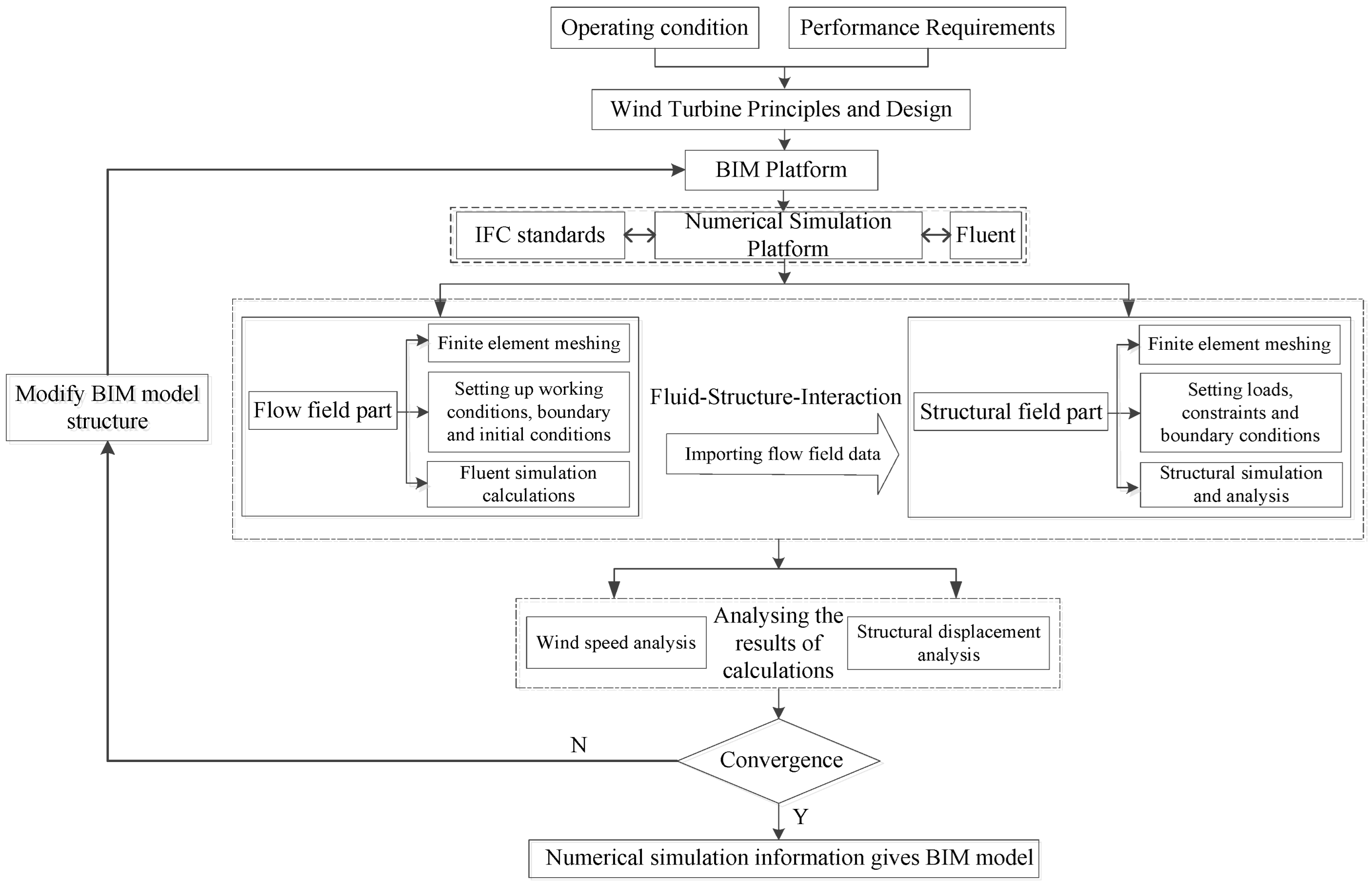
2.1.1. BIM+ Numerical Simulation Analysis Framework

The structure of wind turbine blades is complex. To meet the complex and variable design needs and assess the performance of blades under various wind loads, this paper performs a performance analysis of wind turbine blades based on BIM forward design. The core workflow comprises five steps:

Step 1: According to the design specification of wind turbine blades, a 3D integrated model of the blades is built in the BIM platform.

Step 2: The geometric and attribute information in BIM model is transferred to numerical simulation platform via a standardized data interface.

Step 3: The numerical calculation of the flow field part is completed on the numerical simulation platform, and the flow field data is then imported into the structural field for numerical calculation.

Step 4: The fluid–structure interaction (FSI) is employed to calculate and analyze the blades’ pressure distribution and displacement under wind load effects.

Step 5: The simulation results are iteratively integrated into the BIM model through a bidirectional data linkage, enabling parametric updates and enhancing the model’s informational depth.

The specific analysis framework is shown in Figure 1.

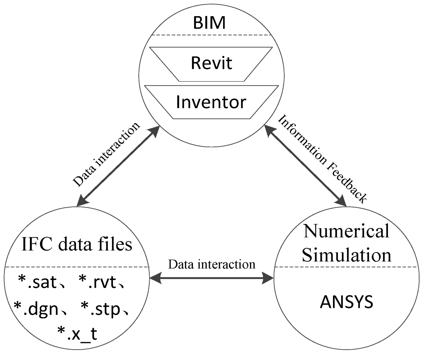
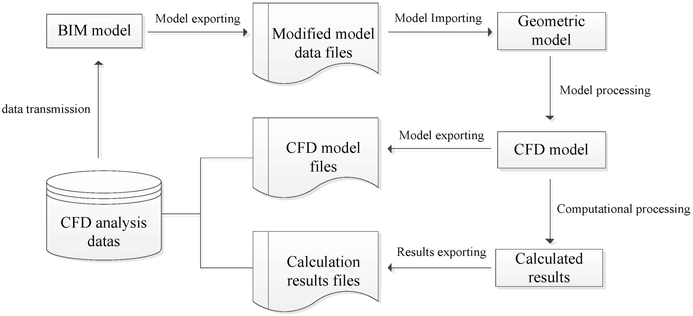
2.1.2. BIM and Numerical Simulation Data Transfer Method

BIM, as an advanced object-based modeling and collaboration platform [32], provides detailed physical parameter support for numerical simulation on wind turbines. The integration of BIM and numerical simulation enables the use of specific numerical algorithms to explore the potential performance of design solution in a hypothetical scenario, thus creating a highly integrated and accurate design environment for wind turbine blades. There are three main ways to transfer data between the BIM platform and the numerical simulation platform [33]: Firstly, data transfer is carried out through internal interfaces for data transmission, in which different BIM and numerical simulation software are often produced by different development teams or companies with varying internal interface standards. This situation leads to the fact that the internal interface of one software may not be directly compatible with the internal interfaces of other software [31], thereby limiting the breadth and flexibility of data interaction. Secondly, data transmission is carried out through external programming or plug-ins, which require users to have specific programming skills or at least understand the configuration and use of plug-ins, which may pose a big challenge for users with non-technical backgrounds. Thirdly, data transmission is carried out through the export of intermediate format files, which makes the data interaction between different software no longer limited to a specific internal interface. Therefore, this paper adopts the export of intermediate format files for data transfer.

The IFC (Industry Foundation Class) standard is a fundamental standard for data expression and information sharing, specifically for the construction industry [34]. A variety of BIM software can export their intermediate format files for numerical simulation and analysis, thereby solving the problem of information isolation at different stages of the project. The data transfer path based on the IFC standard is shown in Figure 2. In the figure, “*” represents a wildcard for any filename.

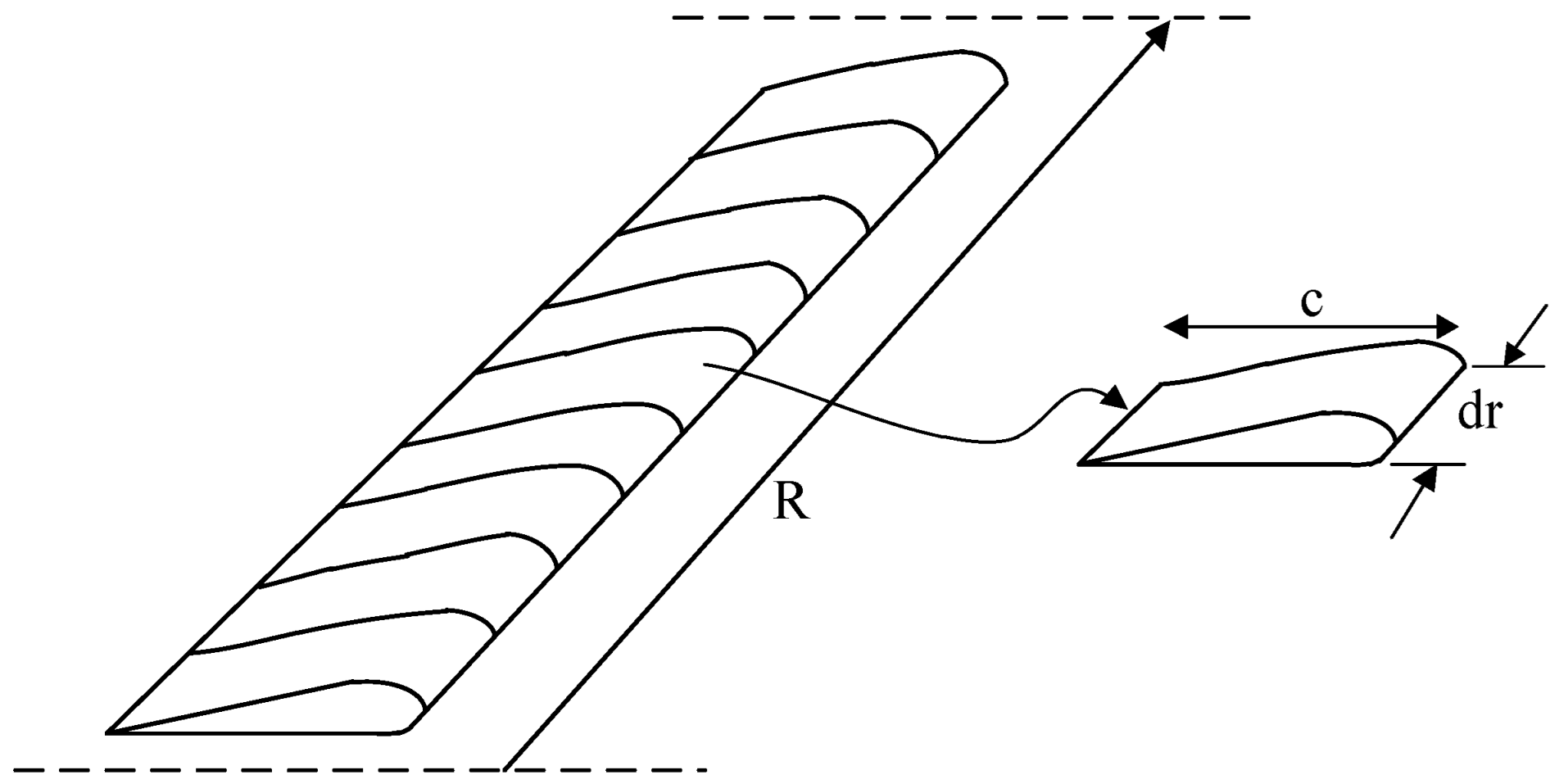
2.2. Blade-Element Theory

The blade-element theory is a mathematical model commonly used in the wind power field [35]. This model follows the classical formulation of blade-element momentum (BEM) theory, which is a foundational methodology for wind turbine aerodynamics as described by Manwell et al. [36]. The theory assumes that a wind turbine blade of finite length is divided into many micro-segments along the spreading direction, and each unit micro-segment is called a blade-element. Each blade-element can be considered as a 2D airfoil. It is assumed that there is no interference between the different blade-elements and that the blade-element unit itself is small enough to be equivalent to an airfoil, as shown in Figure 3. Figure 3 is independently drafted based on the generic framework of blade-element theory, and it is consistent with the classical formulation by Manwell et al.

In Figure 3, R is the rotor radius; c is the chord length; and dr is the unit micro-segment of the blade.

The blade-element theory applies a differential method to reduce the blade into an organic composition of several airfoil sections, which solves the generality problem of wind turbine blade design parameters [37]. It provides new ideas for the design and manufacture of blades.

The basic assumptions of the blade-element theory are as follows:

(1) Interference between neighboring blade-elements along the direction of blade spread is not considered.

(2) The force acting on each blade-element is determined only by the aerodynamic properties of the blade-element’s airfoil.

2.3. CFD Numerical Simulation

The research on the aerodynamic characteristics of wind turbines mainly involves theoretical analysis and experimental tests. With the improvement of computer performance, the theory based on CFD has become the mainstream of theoretical analysis. The CFD method is a simulation method formed by the cross-fertilization of computer technology and numerical computation technology, which is used to simulate actual fluid flow situations. The virtual simulation of blades using the CFD method can accurately and quickly study their aerodynamic characteristics.

2.3.1. Fluid Control Equations

This study accounts for the actual operating environment of wind turbines. Under the idealized conditions, the fluid is considered a continuous and uniform medium, and its volume remains unchanged during flow process, which is regarded as incompressible. In addition, to simplify the analysis, the influence of temperature fluctuations on the fluid properties is ignored, and the energy equation is excluded, thereby focusing on the basic characteristics of fluid dynamics. In the field of CFD, the Navier–Stokes equations [38] are widely used for high-precision numerical simulations of complex fluid problems and are chosen to simulate the state of wind farm. The governing equations of the fluid flow are as follows.

The continuity equation:

$${\displaystyle \frac{\partial {\rho }_f}{\partial t}}+\nabla ·\left({\rho }_{f}v\right)=0$$

(1)

The Navier–Stokes equation:

$${\displaystyle \frac{\partial \left({\rho }_{f}v\right)}{\partial t}}+\nabla ·\left({\rho }_{f}vv-{\tau }_f\right)=f_f$$

(2)

where, ${\rho }_f$ is fluid density; $v$is velocity vector; $f_f$ is volumetric force vector; ${\tau }_f$ is shearing force tensor, equation for calculation is:

$${\tau }_f=\left(-p+\mu \nabla ·v\right)I+2\mu e$$

(3)

where, $p$ is fluid pressure; $\mu$ is dynamic viscosity; $I$ is unit matrix; $e$ is velocity stress tensor, $e=\left(\mathit{\nabla }v+\mathit{\nabla }{v}^T\right)/2$.

2.3.2. Solid Control Equations

According to Newton’s second law of Motion—Force and Acceleration, the conservation equation of solid part is derived:

$${\rho }_s{\ddot{d}}_s=\nabla ·{\sigma }_s+f_s$$

(4)

where,${\rho }_s$ is solid density; ${\ddot{d}}_s$ is local acceleration vectors in the solid domain; ${\sigma }_s$ is Cauchy stress tensor; $f_s$ is volumetric force vector.

2.3.3. Fluid-Solid Coupling Boundary Conditions

At the fluid-solid interaction boundary, physical quantities such as displacements and stresses in the flow field and the structural field must satisfy the principle of equivalence or conservation to ensure that the physical states at the interface of the two match and are conserved. The conservation equation is derived:

$$\left\{\begin{array}{c}{\tau }_f{n}_f={\tau }_s{n}_s\\ d_f=d_s\\ q_f=q_s\\ T_f=T_s\end{array}\right.$$

(5)

where, $\tau$ is the stress; $d$ is the displacement; $q$ is the heat flux; $T$ is the temperature; $n$ is the directional cosine. The subscript $f$ is the fluid; The subscript $s$ is the solid.

3. Constructing BIM Model of Blades

3.1. Design Overview

The wind turbines comprise several key components, including blades, hubs, spindles, gearboxes, generators and so on. These components interact with each other and work together to convert wind energy into electrical energy. When analyzing the performance of the blades, placement within the complete system context becomes essential. Thus, it is first necessary to construct a 3D model of wind turbine as a whole, and then the performance analysis of the blade structure can be performed.

3.1.1. Wind Turbine Design Parameters

In this paper, the TJ 2.2 MW wind turbine is taken as an example for modeling. The relevant design parameters are shown in

Table 1. Relevant parameters for wind turbine design.

Parameters	Numerical Value
Rated power/MW	2.2
Rated wind speed/m/s	12
Cut-in wind speed/m/s	3
Cut-out wind speed/m/s	25
Number of blades	3
Rotor diameter, Hub diameter/m	98.5, 4
Length of blade/m	47.3
Tower height/m	65

. The rated power of this turbine is 2.2 MW (the maximum continuous electrical output under stable working conditions), which is achieved at a rated wind speed of 12 m/s (the minimum wind speed required for the turbine to generate the nominal power). The operational wind speed range spans from a cut-in speed of 3 m/s (the minimum wind speed required to initiate power generation) to a cut-out speed of 25 m/s (the maximum safe wind speed before automatic shutdown).

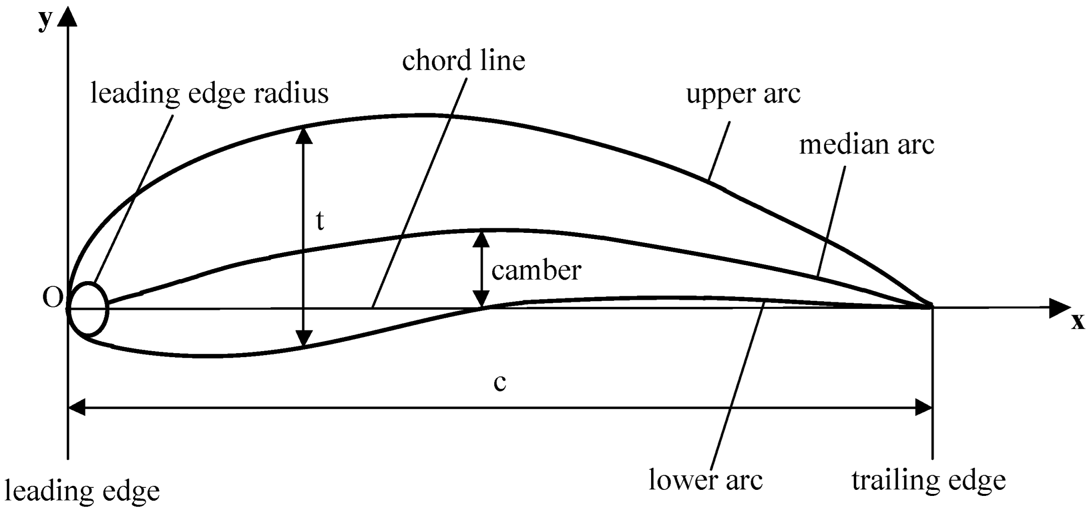
3.1.2. Airfoil Design Parameters

According to Blade-element theory, the TJ 2.2 MW wind turbine blade is divided into 19 blade-elements along the spreading direction, and its related parameters are shown in Appendix A.

3.2. Pre-Processing for Constructing BIM Models

Before constructing the BIM model, it is necessary to have the parameters of the wind turbine blade type for this case study and to process the coordinate data generated from the parameters. Firstly, the 2D coordinates of an airfoil section are obtained from the relevant parameters of blades, and these coordinates are then exported by the specialized airfoil design software XFOIL 6.99. Then, the 2D coordinates need to be processed to obtain the spatial coordinates of the discrete points of each section. In the data processing work, this paper proposes a method for efficiently processing blade data using MATLAB, aiming to enhance the efficiency of blade design and ensure the accuracy of the data used in constructing BIM model. Figure 4 shows this pre-modeling workflow, which comprises three main steps described below.

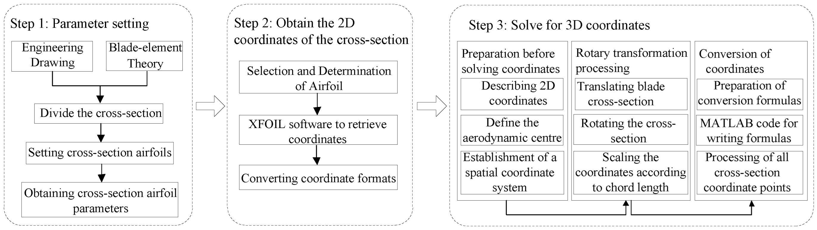
3.2.1. Parameter Setting

According to engineering drawings and blade-element theory, the basic unit of a blade consists of blade-element airfoils. The diameter of rotating swept plane of blades is referred to as the airfoil spread, which is the diameter of wind turbine’s rotation essentially. The contour curve of cross-section of wind turbine blades, perpendicular to the airfoil direction, is known as the airfoil shape.

The airfoil parameters include airfoil geometry parameters and airfoil aerodynamic [39] coefficients. Airfoils are generally long and thin, with a rounded leading edge and a blunt or pointed trailing edge. The geometric parameters describing airfoil include chord line, chord (c), thickness (t), camber, leading edge, leading edge radius, trailing edge and arcs (upper, mid and lower), as shown in Figure 5.

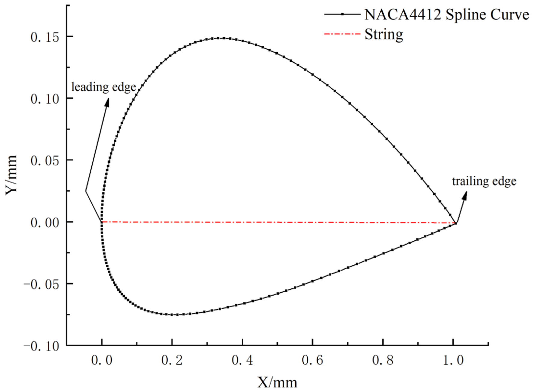
3.2.2. Obtaining 2D Coordinates of Cross-Section

When designing wind turbine blades, several key elements must be considered comprehensively [40], including blade mounting configuration standards, blade twisting angles, system lift-to-drag ratios, thicknesses, materials and so on. This work encompasses dynamics, electrical automation, blade loading, airfoil geometry parameters, composite structures, aerodynamic profile design, airfoil design and other technical functions related to the efficiency of wind turbines. It is critical to select the appropriate airfoil. XFOIL is a commonly used simulation software in airfoil design, which features a specific airfoil database, and a group of 2D coordinates of an airfoil cross-section can be obtained by inputting the required airfoil. The American NACA four-digit airfoil is widely used [41] in wind turbine blade design due to its low drag coefficient and high lift coefficient. Taking the NACA44XX series airfoil as an example, 19 groups of 2D coordinates of blade sections are obtained. There are a total of 160 points for each section. The 2D coordinate file is imported into Inventor 2018, and a spline curve is created based on point coordinates. Then, the 2D coordinate spline curve graph of an airfoil cross-section can be obtained. Taking the NACA4412 cross-section (r = 30.46 m, t/c = 12.22%) as an example, it is shown in Figure 6.

In Figure 6, the horizontal coordinate X represents the transverse coordinate of airfoil, and the vertical coordinate Y represents the longitudinal coordinate of airfoil. Wind turbine blades are spatially streamlined and have a complex spatial structure; therefore, it is necessary to perform a coordinate transformation of 2D coordinates to obtain 3D coordinates to create a 3D model.

3.2.3. Solving for 3D Coordinates

In the 3D spatial coordinate system, the coordinates of each blade discrete point can be represented in space, which is convenient for observing the positional relationship of each blade cross-section in space and understanding the streamlined structure of blades more intuitively. Therefore, it is necessary to establish an appropriate 3D spatial coordinate system to determine the spatial coordinates of discrete points on each blade section. The root of the blades, i.e., the cross-section of blades with a radius of 0, is defined as the XOY plane, and the direction along the Z-axis is represented as the blade extension direction. Then, the spatial coordinates of discrete points on each blade section are represented as $\left(x,y,z\right)$.

The steps for solving the blade spatial coordinates are as follows:

Step 1: The upper and lower chord coordinates of airfoil are obtained by XFOIL software, denoted as $\left(x0,y0\right)$.

Step 2: The aerodynamic center of the blade section with radius 0 is defined as the origin, which enables the 2D airfoil coordinates to be obtained with the aerodynamic center as the origin, denoted as $\left(x\prime ,y\prime \right)$.

Step 3: The 2D coordinates are processed by rotational transformation to obtain 3D spatial coordinates.

The specific solution steps of rotational transformation process are as follows:

Step 1: The blade cross-section is translated until the aerodynamic center of the airfoil with a cross-section radius of 0 is the origin of the coordinates.

Step 2: The coordinates of each blade airfoil are rotated according to the twisting angle of each cross-section.

Step 3: The airfoil coordinates are scaled according to the chord length of each part.

The final formula for this process is

$$x^{\prime }=c{\displaystyle \frac{\left|\chi -{\chi }_0\right|}{x-x_0}}\sqrt{{\left(x-x_0\right)}^2+z^2}\cos \left(\arctan {\displaystyle \frac{z}{x-x_0}}+\beta \right)$$

(6)

$$z^{\prime }=c{\displaystyle \frac{\left|\chi -{\chi }_0\right|}{x-x_0}}\sqrt{{\left(x-x_0\right)}^2+z^2}\sin \left(\arctan {\displaystyle \frac{z}{x-x_0}}+\beta \right)$$

(7)

$$y^{\prime }=r$$

(8)

where, $x,z$ are airfoil normalized coordinates;$x_0$ represents cross-section aerodynamic center coordinates; $x^{\prime }{,y}^{\prime },z^{\prime }$ are transformed section coordinates; $c$ is chord length; $\beta$ is twist angle; $r$ is radius.

Due to the huge number of discrete coordinate points, the number of discrete points obtained from a single cross-section obtained from XFOIL is as many as 160 points. The MATLAB software offers excellent programming functions and supports efficient data batch interpolation and arithmetic [42]. To optimize the efficiency of converting 2D to 3D coordinates, this study uses MATLAB to write Formulas (6)–(8) to batch convert 2D coordinates into 3D coordinates. The large amount of data obtained after processing is consolidated into a single file to facilitate the subsequent modeling process.

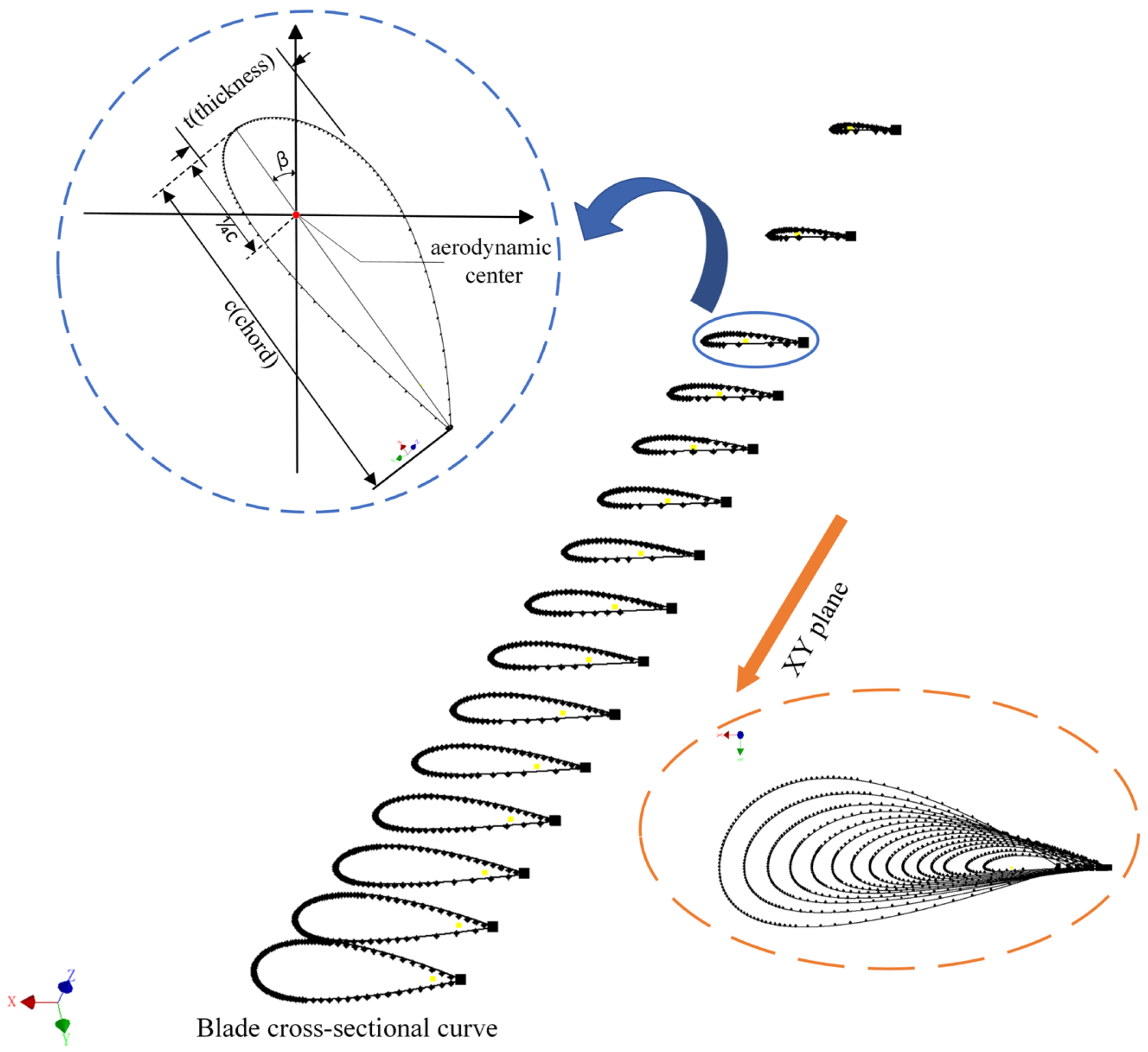
3.3. Generating Blade Cross-Section Curves

The spatial coordinates of the discrete points on blade cross-section are obtained using XFOIL software. The obtained file data are then imported into Autodesk Inventor 2018, and the blade cross-section curve can be generated by using the operation of creating a spline curve.

Specific operation methods are as follows:

Step 1: Use Inventor 2018 to select the “Create 3D Sketch Model” option and then import the point coordinate file.

Step 2: The software fits discrete point spatial coordinates and generates a spline curve, ultimately obtaining an exact spline curve for each blade section.

The generated spline curve and position of the blade cross-section are shown in Figure 7, which illustrates the parametric expression of a specific cross-section and the cross-section viewed in the XY plane.

In Figure 7, the yellow points denote the aerodynamic center locus along the blade extension direction (Z-axis). Each point represents the aerodynamic center of its local cross-section, forming the reference axis for aerodynamic analysis. This differs from discrete points defining the cross-section shape (black points).

3.4. Generating the Entity Model of Blade

3.4.1. Generating Preliminary Model

There are many ways of modeling blades, such as through points, curves, mesh curves and so on. Although all of these methods can construct a blade 3D model, the model accuracy varies greatly, and some of the blades obtained by these methods may even have obvious structural defects. The blade model obtained through the spline curve operation is relatively smooth compared to the other methods mentioned above, and its accuracy is relatively high because the process is carried out by the spline curve generated from multiple 3D discrete points. Therefore, this paper employs the method of spline curves to construct blade BIM model. The process is as follows:

Within Autodesk Inventor, the lofting operation is used, with the Z-axis direction serving as the direction of the leading string for the cross-sectional spline curve. The blade 3D entity model is created by clicking on the spline curves generated from each cross-section along the direction of lead strings in a sequential manner.

3.4.2. Checking and Trimming of Blade Model Surfaces

It is crucial to ensure the smoothness of the surface during model simulation [43], especially when dealing with complex surfaces such as blades. The model obtained by using Inventor’s loft operation is relatively accurate and smooth. However, because the surface is generated based on multiple spline curves, there are transition parts, and the curves of the transition parts vary greatly, resulting in the problem of unsmooth surface obtained by lofting. Therefore, it is required to check and trim the smoothness of blade surface to ensure streamlined lines and quality.

The detailed steps below explain how to check and trim the smoothness of the blade model surface:

Step 1: Load the blade 3D model using Inventor and identify areas with large curvature variations that may not be smooth by visual inspection or by using relevant analysis tools.

Step 2: Select a few key curves near identified unsmooth areas.

Step 3: For the selected curves, find the fitting points that may lead to an unsmooth phenomenon and adjust them, especially where the curvature changes most dramatically. Try to improve the curve smoothness by shifting the position of these points;

Step 4: After adjusting fit points, refit the curve using the “Recalculate” or “Update” function in Inventor software. If the curve is part of a surface, refit the entire surface to ensure that the entire surface is smooth.

Step 5: Use visualization tools in Inventor to check if the refitted curves and surfaces are as smooth as expected. If there is still an unsmooth problem, repeat steps three to five until satisfactory smoothness is achieved. In the final step, the validation and testing of designed blades are completed by measuring, observing or conducting performance tests.

A brief flowchart of blade check and trimming process is shown in Figure 8. After surface trimming, the 3D entity model of the TJ 2.2 MW wind turbine blades is constructed in Inventor software using the loft operation, as shown in Figure 9.

4. Numerical Simulation and Results Analysis of Blades

4.1. Setting Parameters and Meshing

4.1.1. Working Condition Parameters

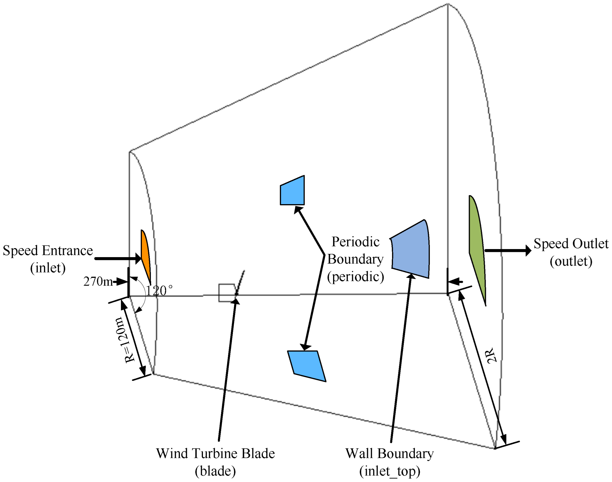
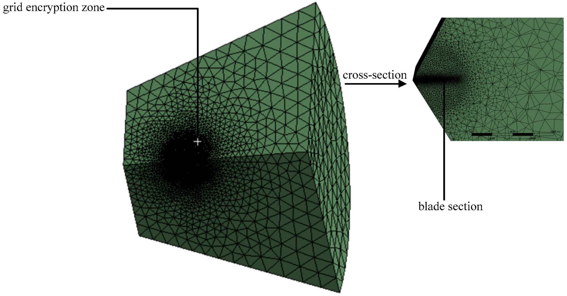
In the actual operation of wind turbines, wind speed constantly varies, which causes the wind load on blades to change dynamically [4]. By analyzing the dynamic changes in blade structure under different wind speeds, it becomes possible to better understand the force characteristics of blades in complex wind conditions and to develop more scientific and reasonable blade maintenance strategies, thereby providing reference directions for designers and maintenance personnel of wind turbines. Based on the actual working conditions of wind turbines, three simulation conditions with inlet wind speeds are selected for numerical simulation under different wind speed conditions. The specific working condition parameters are shown in

Table 2. Parameters of simulated working conditions.

Simulated Working Conditions	Inlet Wind Speed/m/s	Outlet Pressure/Pa
Low wind speed	8	101,325
Rated wind speed	12	101,325
High wind speed	25	101,325

.

4.1.2. CFD Modeling

The blade BIM model is imported into ANSYS 2022 R1-Design Model for model pre-processing. Before performing numerical simulations of wind turbine blades, it is essential to establish the fluid domain. The design of the shape and size of the fluid domain is crucial. Based on the actual working environment of wind turbines, this study uses a frustum shape instead of a rectangular domain because its conical structure better matches the wind speed gradient distribution, thereby reducing artificial flow field distortion. Its downstream expansion structure lowers the risk of backflow at the outlet, while the upstream contraction minimizes the disturbance of the inlet wind direction. The cross-sectional size of the fluid domain is $R_{min}=$ 120 m and $R_{max}$ = 240 m, with a height of 270 m. The minimum cross-sectional radius exceeds twice the blade length, mitigating pressure oscillations caused by small domain sizes. Furthermore, since the wind turbine blades are distributed in a circular array, only one blade CFD model is modeled, and then the number of array distributions is 3, with the Z-axis as the central axis in the final Fluent solver calculation. The specific parameters of the fluid computational domain and boundary conditions in the pre-processing are shown in Figure 10. The wind farm is selected as the target body, and Boolean operation is performed on the flow domain with the solid model of the wind turbine blades as the tool body to obtain the required fluid domain model.

Meshing is required after pre-processing. Face meshing is applied to the entire fluid domain, with a tetrahedral mesh form. The face meshing size of blades is set to be no larger than 0.3 m, and the mesh is encrypted in the transition region where the flow domain is in contact with blades. In the end, a total of about 351,769 meshes are divided, and 69,960 nodes are generated with an average mesh quality of 0.82, indicating that this mesh is of good quality [44]. The overall effect of the obtained fluid domain meshing is shown in Figure 11.

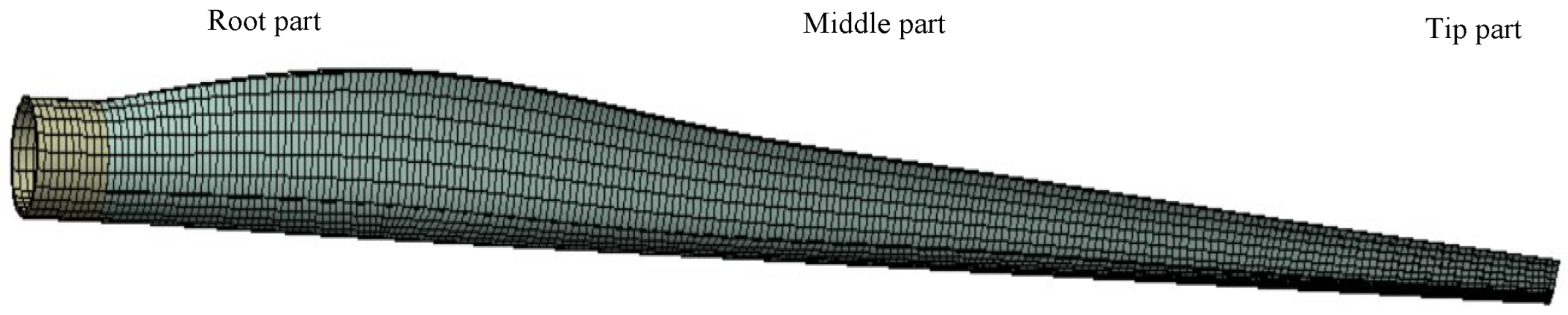
4.1.3. Finite Element Modeling of Blades

After establishing the finite element model in the fluid domain, the shared topological relationship between the flow field and the structural field is set at the same node. A Static Structural module is then created through the Workbench 2022 R1 platform, allowing flow field data calculated in the Fluent module to be transferred to the solid structure for the analysis of blade structure. The fluid domain is suppressed, and only blade structure is analyzed. The meshing strategy uses the face meshing (face mapping mesh) drawing method, and the size of the face mesh is set to be no larger than 0.2 m. Finally, a total of 5307 meshes are divided, and 5138 nodes are generated, with an average mesh quality of 0.84, indicating that the mesh quality is good [44]. The blade finite element model is shown in Figure 12.

In Figure 12, color segmentation corresponds to different functional domains: yellow denotes the root cylinder (pure mechanical interface), while green marks the aerodynamic airfoil area that requires a specialized flow-sensitive meshing.

4.2. Mesh Independence Verification

To mitigate the effects of discretization errors on computational results, this study performs a systematic mesh independence verification. For the aerodynamic performance prediction of a 2.2 MW wind turbine under rated conditions (wind speed of 12 m/s), an independence verification is carried out using a progressive mesh refinement strategy. The computational domain is divided into three mesh levels, with the relevant parameters detailed in

Table 3. Mesh parameters and results under different levels.

Mesh Level	Number of Nodes	${\mathit{C}}_{\mathit{p}}$	${\mathit{C}}_{\mathit{t}}$	Computational Time (h)	Mesh Quality (Min. Orthogonality)
Coarse	34,870	0.458	0.083	1.8	0.35
Medium	69,960	0.478	0.089	4.5	0.42
Fine	142,530	0.483	0.091	20.1	0.48
Benchmark	-	0.486	0.092	-	-

. The convergence behavior of the power coefficient ($C_p$) and torque coefficient ($C_t$) is primarily focused on, with Richardson extrapolation [45] used to compute extrapolated benchmark values for enhanced accuracy in mesh convergence assessment.

Convergence analysis under different mesh levels is performed using the parameters detailed in

Table 4. Convergence analysis under different mesh levels.

Mesh Comparison	${∆\mathit{C}}_{\mathit{p}}$ (%)	${∆\mathit{C}}_{\mathit{t}}$ (%)	Convergence
Coarse → Medium	+7.23	+4.37	Not converged
Medium → Fine	+2.25	+1.05	Converged
Fine → Benchmark	+1.10	+0.62	Fully converged

. The result shows that when refining from the coarse to the medium mesh level, $C_p$ increases by 4.37% (from 0.458 to 0.478) and $C_t$ rises by 7.23% (from 0.083 to 0.089), which indicates that the coarse mesh underestimates tip losses. Further refinement to the fine mesh level results in significantly diminished parameter variations (${∆C}_p$ = 1.05%, ${∆C}_t$ = 2.25%), meeting the convergence threshold criteria. Considering both calculation accuracy and efficiency, the optimal model performance occurs when the number of nodes is 69,960. At this point, the calculated value is relatively close to Richardson extrapolation value, and the mesh convergence is good.

4.3. Numerical Results Analysis

4.3.1. Wind Pressure Analysis

The surface of wind turbine blades is affected to different degrees under varying incoming wind speeds. In this study, the numerical simulation of the Fluent module is applied to obtain the distribution of wind pressure on both windward and leeward surfaces of blades under different incoming wind speeds, as shown in Figure 13. Figure 13 indicates the following: (1) Windward side: The pressure values are predominantly positive. The maximum pressure occurs at the leading edge of the blade tip and at the middle part. The pressure on the leading edge of the blades is obviously greater than the pressure on the trailing edge, which is the reason for the rotating motion of the blades. (2) Leeward side: The pressure values are primarily negative. The maximum value of negative pressure is distributed at the tip of the blades in low and rated wind speeds, and the distribution area of the maximum value of negative pressure is enlarged in the case of high wind speed. As the wind speed increases, the negative pressure values and negative pressure area of blades also increase, which will lead to an increased risk of blade instability and failure. (3) Speed–pressure relationship: As the wind speed increases, the overall pressure on the blades increases, with the maximum positive pressure on the windward side reaching 4.96 kPa and the maximum negative pressure on the leeward side reaching 6.28 kPa, both of which occur when the wind speed is 25 m/s. The average leading–trailing edge pressure difference increases with wind speed, peaking at 4.95 kPa at a wind speed of 25 m/s, which can influence the blades’ structural stability.

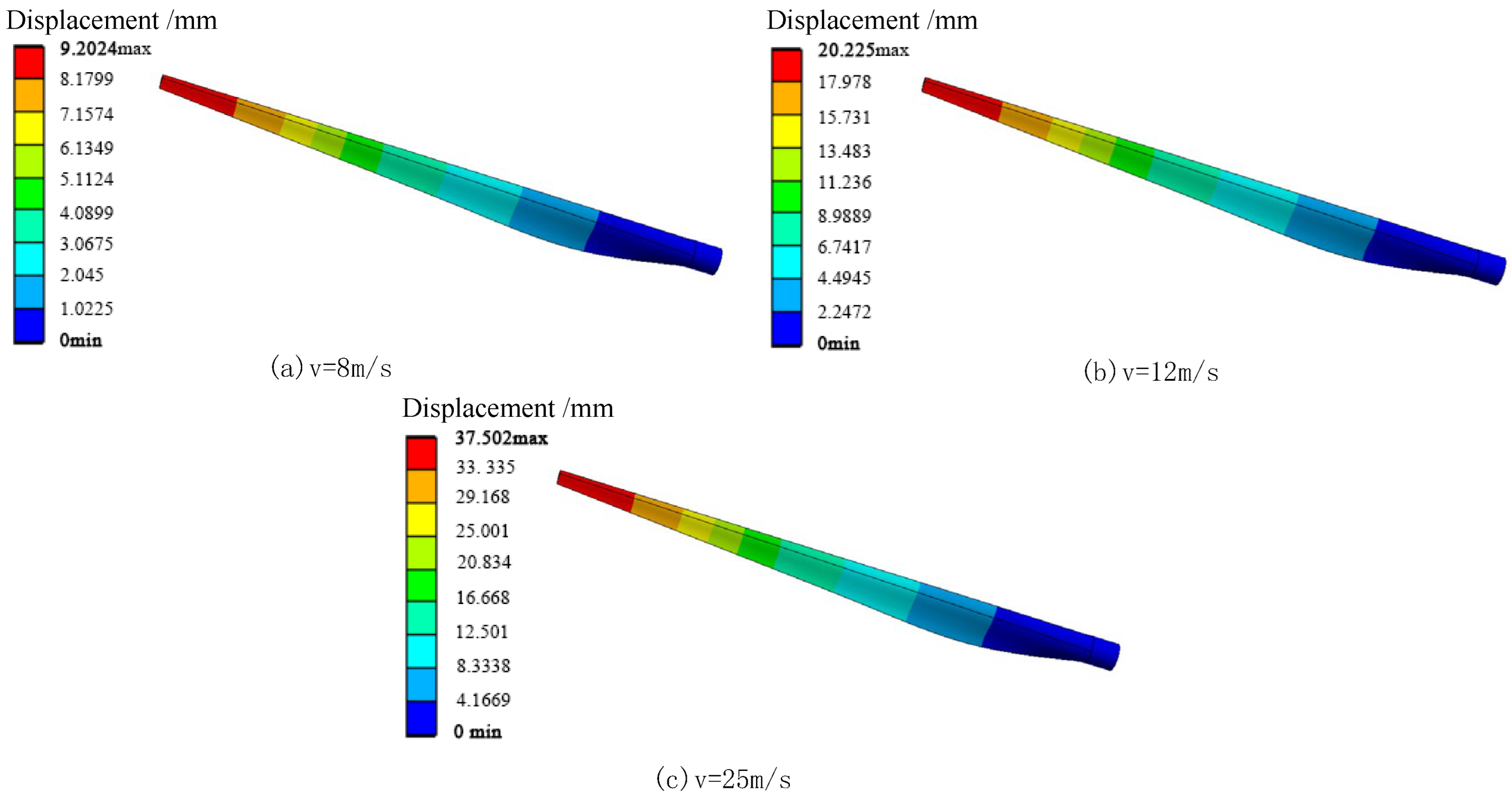
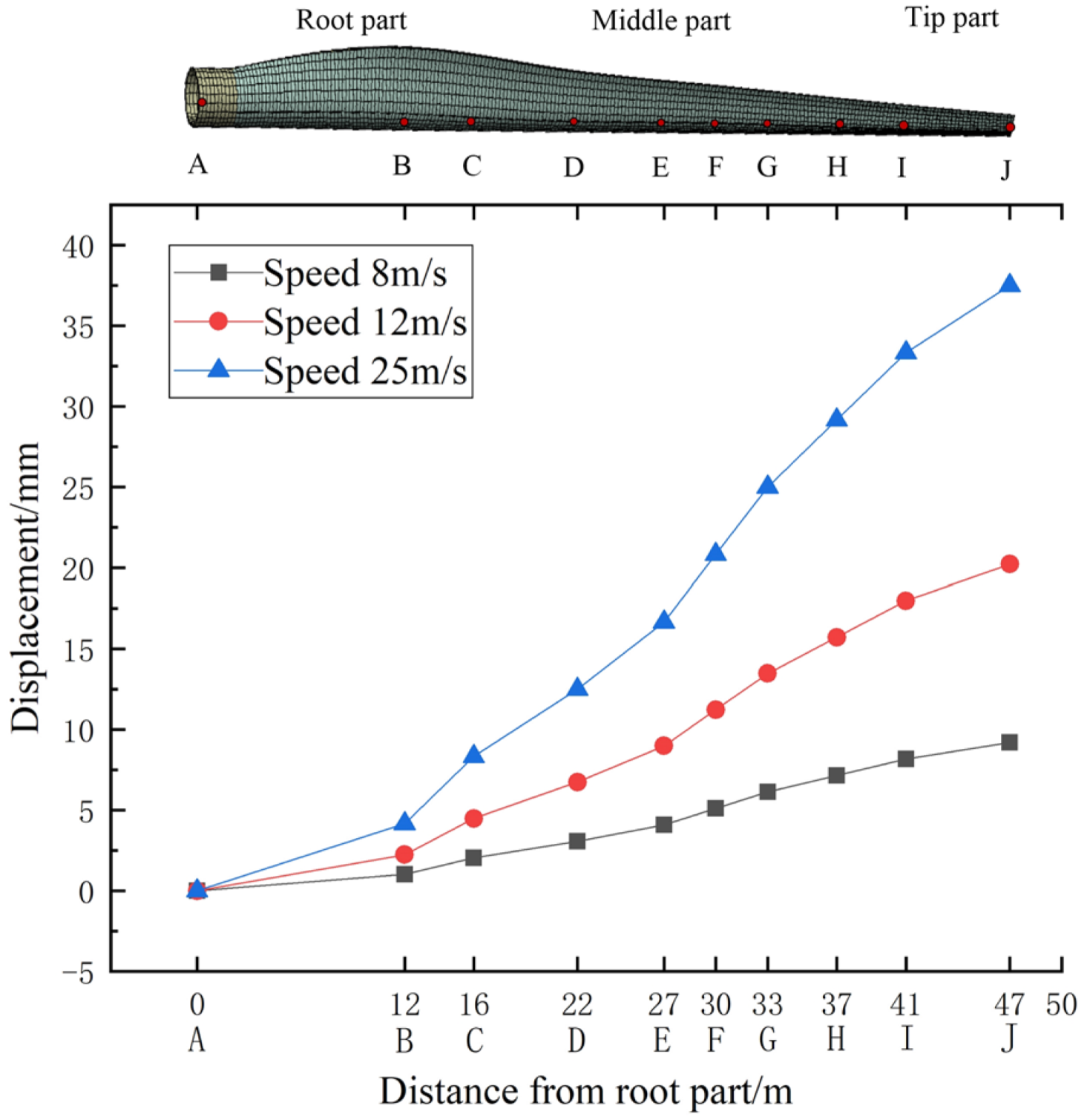
4.3.2. Blade Structure Displacement Analysis

Under different wind speed conditions, the blades will be subjected to varying degrees of wind loads, leading to swaying vibrations where different sections exhibit varying vibration amplitudes. Excessive swaying displacement may even cause permanent deformation of blade structure, impacting the aerodynamic performance of wind turbines and reducing power generation efficiency. It also hinders the elasticity recovery of blades, further increasing fatigue damage. The numerical simulation by Static Structural to obtain the displacement of blade structure under different wind speed conditions is shown in Figure 14. Figure 14 indicates the following: Under different conditions, the maximum displacement occurs at the blade tip part, and the displacement values show a decreasing trend from the tip to root, which suggests that the structural thickness of different blade sections should be considered in the design process. Furthermore, the displacement amplitude of each characteristic point of blades under different working conditions is compared and analyzed, as seen in Figure 15: The overall displacement of blades under each working condition increases with wind speed. The rate of change at the blade tip and middle displacements increases from 1.02 to 4.16, and the growth rate of maximum blade displacement between neighboring wind speeds ranges from 1.20 to 1.94. Therefore, the influence of wind speed on the safety and stability of the structure itself should not be ignored, and the excessive wind load on blades under extreme conditions may cause sudden increases in the displacement at the blade tip and middle part, potentially leading to blade fracture damage.

5. Verification and Application of the Numerical Results

5.1. Comparative Validation of the Numerical Results

Since the proposed BIM forward design combined with the CFD numerical simulation method is based on computer simulation results, and the wind speed in external environment is constantly changing, it is currently impossible to directly verify the performance data of blades in the real world. As an alternative validation approach, this study employs a benchmarking strategy by cross-referencing our model predictions with empirical data from comparable peer-reviewed investigations. These reference studies are selected based on similar characteristics, such as comparing pressure and deformation values under the same conditions. Through comparative analysis, we observe the deviation situation to determine whether it is within an acceptable range. This comparative analysis provides a relatively reliable basis for assessing the model’s credibility in the absence of specific performance data for the actual environment.

5.1.1. Verification of Wind Pressure Analysis Results

To rigorously assess the reliability of the analysis results, a systematic verification and comparison of the existing literature is conducted. Quantitative comparisons focus on three key aspects of wind pressure distribution: the pressure advantage on windward side, the suction characteristics on leeward side, and the relationship between wind speed and pressure. This study is compared with experimental measurements and high-precision calculation reference values. The specific comparison conclusions are as follows.

(1) Windward pressure distribution shows tip/mid-span concentration (4.96 kPa at 25 m/s), aligning with rotating blade test measurements (4.7–5.2 kPa, +5.0% deviation) in boundary layer wind tunnels [46], while leading edge dominance (contributing 60–75% of total driving force) is validated by 3D radial flow simulations capturing the Coriolis-enhanced lift mechanism [47];

(2) Leeward suction characteristics show tip-focused peaks (−6.28 kPa) matching full-scale blade pressure tap data [46] (−6.2 $\pm$ 0.3 kPa, +1.3% deviation). The suction area expansion correlates to a 15–20% increase in the rotating trial [48] and exceeds the DNV GL buckling threshold (−6.0 kPa) for composites. This phenomenon confirms a risk of structural instability.

(3) Wind speed–pressure correlation reveals a leading–trailing edge (ΔP) of 4.95 kPa at 25 m/s, residing within the LES-predicted range (4.8–5.2 kPa, +3.1% deviation) [49].

All core parameters show deviation ($\le$5%) from experimental and computational benchmarks, as indicated in

Table 5. Comparison of pressure simulation values with the literature results.

Parameter	Present Model	Comparison Model	Deviation	Source
Windward pressure	4.96 kPa	4.7 − 5.2 kPa	+5.0%	[46,47]
Leeward suction	−6.28 kPa	6.2 ± 0.3 kPa	+1.3%	[46,48]
ΔP	4.95 kPa	4.8 − 5.2 kPa	+3.1%	[49]

, meeting the validation criterion mandated (<10%) by the IEC standard for wind energy CFD models. Therefore, the results of integrating BIM forward design with CFD for the analysis of blade wind pressure are highly effective.

5.1.2. Verification of Displacement Analysis Results

To assess the reliability of blade structure displacement analysis results, this study compares and verifies the results with those of the other literature. The comparison focuses on two main aspects: the dominance of blade tip displacement and the correlation between wind speed and displacement. The key verification results are as follows:

(1) Maximum displacement consistently occurs at blade tip across all working conditions, aligning with rotating blade test measurements where tip displacement accounts for more than 80% of total displacement [50]. This phenomenon is validated by 3D transient simulations capturing rotational stiffening effects: centrifugal forces increase root stiffness by 35–40% while tip stiffness remains 20–25% of the root value.

(2) Large eddy simulation (LES) by Elias, S. [51] confirms that when the flow separation exceeds 12 m/s, airflow separation reduces aerodynamic damping by 42% and increases the displacement growth rate from 1.15 to 1.82. This matches the observed trend (1.20 $\to$ 1.94). As tip displacement exceeds 15% of the chord length (DNV GL threshold), composite buckling triggers stiffness attenuation. At 25 m/s, the stiffness attenuation reaches 12%, causing the displacement growth rate to exceed the linear prediction by 47%, which is consistent with the displacement surge observed in Figure 15.

A comparative analysis of the literature shows that the combined application of BIM and CFD numerical simulation is effective in the displacement analysis of wind turbine blade structures, as shown in

Table 6. Comparison of displacement simulation values with the literature.

Parameter	Present Model	Comparison Model	Deviation	Source
Displacement distribution	Blade tip	Tip displacement /total (>80%)	Spatial match	[50]
Wind speed displacement	Strong correlation	Strong correlation	Spatial match	[51]

.

5.2. Coupling of Numerical Simulation Results with BIM Model

The verification results have demonstrated the feasibility of integrating BIM forward design with CFD numerical simulation for the performance analysis of wind turbine blades. This method can construct a two-way collaborative framework, guiding the design process.

Through the fluid–structure coupling simulation process of wind turbine blades, the blade damage mechanism when subjected to wind load is revealed, and numerical simulation results can be attached to the corresponding components of the BIM model as additional information for integrating simulation results with BIM data. The information transfer process is shown in Figure 16. Using the numerical simulation results integrated into the BIM model, further analyses and applications can be performed. For instance, the safety of blade structure can be evaluated to optimize the blade design and provide designers with design optimization directions. Specifically, in this study, the maximum wind load positions at the blade tip and middle part can be obtained through wind pressure analysis results. Then, the pressure information can be added to the corresponding BIM component attributes. During the production design phase, different thicknesses can be set for different blade parts according to the results to adapt to a variety of wind speed environments and achieve the purpose of safe operation and cost savings.

6. Conclusions

As a critical component of wind turbines, blade performance analysis is essential to ensuring safe operation. This study performs numerical simulation analysis of wind turbine blades based on BIM forward design, providing model support for blade performance analysis process. Furthermore, based on the CFD calculation method, the blade performance under different wind speed conditions is analyzed. The numerical simulation results indicate the following: The influence of wind load is an important factor in blade damage, and an increase in wind speed will increase the negative pressure on blades, leading to instability and potential damage. Under different wind speeds, the tip and middle swing displacement of blades is the greatest, reaching a maximum of 37.50 mm in extreme conditions, which poses a risk of fracture damage. Therefore, it is crucial to select the appropriate materials and assign reasonable thicknesses to these areas during the design process. For the complex blade shape, this paper provides a detailed description of the modeling method with an example to offer clear design guidelines. This approach can be replicated in the design of other types of wind turbine models. The BIM model combined with the CFD numerical analysis method has a wide range of applicability, and its application in the field of wind power broadens new ideas for blade performance analysis applying it. In addition, the numerical simulation results can be exported and applied to BIM model design, serving as a reference for model design and optimization to prevent frequent blade damage.

Although this study has some reference significance for blade design optimization, certain limitations cannot be ignored. As the primary focus is to explore the feasibility of integrating BIM with CFD for the performance analysis of wind turbine blades, the analysis of blade performance is necessarily limited in scope. Future work will build upon this foundation to conduct a more comprehensive analysis, incorporating dynamic analysis to capture blade behavior over time. Furthermore, this study does not deeply investigate methods for embedding blade analysis results within the BIM model. While a practical implementation approach is proposed, the redesign and optimization processes based on these results are not subjected to detailed examination. In subsequent research, a comparative analysis of the model before and after optimization will be performed to verify the effectiveness of integrating BIM with CFD numerical simulation for blade optimization.

References

1. Hannan, M.A.; Al-Shetwi, A.Q.; Mollik, M.S.; Ker, P.J.; Mannan, M.; Mansor, M.; Al-Masri, H.M.K.; Mahlia, T.M.I. Wind energy conversions, controls, and applications: A review for sustainable technologies and directions. Sustainability 2023, 15, 3986. [Google Scholar] [CrossRef]
2. Badger, J.; Volker, P.J.H. Efficient large-scale wind turbine deployment can meet global electricity generation needs. Proc. Natl. Acad. Sci. USA 2017, 114, E8945. [Google Scholar] [CrossRef] [PubMed]
3. Verma, A.S.; Yan, J.; Hu, W.; Jiang, Z.; Shi, W.; Teuwen, J.J. A review of impact loads on composite wind turbine blades: Impact threats and classification. Renew. Sustain. Energy Rev. 2023, 178, 113261. [Google Scholar] [CrossRef]
4. Dai, J.; Li, M.; Chen, H.; He, T.; Zhang, F. Progress and challenges on blade load research of large-scale wind turbines. Renew. Energy 2022, 196, 482–496. [Google Scholar] [CrossRef]
5. Schubel, P.J.; Crossley, R.J. Wind turbine blade design. Energies 2012, 5, 3425–3449. [Google Scholar] [CrossRef]
6. Djerrad, A.; Fan, F.; Zhi, X.; Wu, Q. Experimental and FEM analysis of AFRP strengthened short and long steel tube under axial compression. Thin-Walled Struct. 2019, 139, 9–23. [Google Scholar] [CrossRef]
7. Zou, Y.; Zhao, X.; Chen, Q. Comparison of STAR-CCM+ and ANSYS Fluent for simulating indoor airflows. Build. Simul. 2018, 11, 165–174. [Google Scholar] [CrossRef]
8. Zheng, X.; Zhou, Y. A three-dimensional unsteady numerical model on a novel aerogel-based PV/T-PCM system with dynamic heat-transfer mechanism and solar energy harvesting analysis. Appl. Energy 2023, 338, 120899. [Google Scholar] [CrossRef]
9. Dou, J.-H.; Jia, X.; Huang, Z.-X.; Gu, X.-H.; Zheng, Y.-M.; Ma, B.; Xiao, Q.-Q. Theoretical and numerical simulation study on jet formation and penetration of different liner structures driven by electromagnetic pressure. Def. Technol. 2021, 17, 846–858. [Google Scholar] [CrossRef]
10. Rhakasywi, D.; Harinaldi; Kosasih, E.A.; Irwansyah, R. Computational and Experimental Study of Heat Transfer on the heat sink with an impinging synthetic jet under Various Excitation Wave. Case Stud. Therm. Eng. 2021, 26, 101106. [Google Scholar] [CrossRef]
11. de Schiara, L.S.; de Ribeiro, G.O. Finite element mesh generation for fracture mechanics in 3D coupled with ansys®: Elliptical cracks and lack of fusion in nozzle welds. J. Braz. Soc. Mech. Sci. Eng. 2016, 38, 253–263. [Google Scholar] [CrossRef]
12. Yang, B.; Liu, B.; Zhu, D.; Zhang, B.; Wang, Z.; Lei, K. Semiautomatic Structural BIM-Model Generation Methodology Using CAD Construction Drawings. J. Comput. Civ. Eng. 2020, 34, 04020006. [Google Scholar] [CrossRef]
13. Cheng, M.-Y.; Soegiono, D.V.; Khitam, A.F. Automated fall risk classification for construction workers using wearable devices, BIM, and optimized hybrid deep learning. Autom. Constr. 2025, 172, 106072. [Google Scholar] [CrossRef]
14. Wang, L.; Lee, J.; Nimawat, J.; Han, K.; Gupta, A. Integrated 4D Design Change Management Model for Construction Projects. J. Constr. Eng. Manag. 2024, 150, 04024023. [Google Scholar] [CrossRef]
15. Wang, H.; Jin, R.; Xu, P.; Gu, J. Generation Method for HVAC Systems Design Schemes in Office Buildings Based on Deep Graph Generative Models. Buildings 2024, 14, 3405. [Google Scholar] [CrossRef]
16. Aghaabbasi, M.; Sabri, S. Potentials of digital twin system for analyzing travel behavior decisions. Travel Behav. Soc. 2025, 38, 100902. [Google Scholar] [CrossRef]
17. Tuhaise, V.V.; Tah, J.H.M.; Abanda, F.H. Technologies for digital twin applications in construction. Autom. Constr. 2023, 152, 104931. [Google Scholar] [CrossRef]
18. Zhang, Z.; Wei, Z.; Court, S.; Yang, L.; Wang, S.; Thirunavukarasu, A.; Zhao, Y. A Review of Digital Twin Technologies for Enhanced Sustainability in the Construction Industry. Buildings 2024, 14, 1113. [Google Scholar] [CrossRef]
19. Tahmasebinia, F.; Lin, L.; Wu, S.; Kang, Y.; Sepesgozar, S. Advanced Energy Performance Modelling: Case Study of an Engineering and Technology Precinct. Buildings 2024, 14, 1774. [Google Scholar] [CrossRef]
20. Lee, Y.-C.; Eastman, C.M.; Solihin, W. Rules and validation processes for interoperable BIM data exchange. J. Comput. Des. Eng. 2021, 8, 97–114. [Google Scholar] [CrossRef]
21. Xu, P.; Liu, P.; Yan, L.; Zhang, Z. Effect of Solder Layer Void Damage on the Temperature of IGBT Modules. Micromachines 2023, 14, 1344. [Google Scholar] [CrossRef] [PubMed]
22. Kang, M.; Bian, J.; Li, B.; Fan, X.; Xi, Y.; Wang, Y.; Liu, Y.; Zhu, Y.; Zi, W. Advanced progress of numerical simulation in drum drying process: Gas–solid flow model and simulation of flow characteristics. Int. Commun. Heat Mass Transf. 2024, 157, 107758. [Google Scholar] [CrossRef]
23. Sayed, M.; Lutz, T.; Krämer, E.; Shayegan, S.; Wüchner, R. Aeroelastic analysis of 10 MW wind turbine using CFD–CSD explicit FSI-coupling approach. J. Fluids Struct. 2019, 87, 354–377. [Google Scholar] [CrossRef]
24. Liu, X.; Lu, C.; Liang, S.; Godbole, A.; Chen, Y. Vibration-induced aerodynamic loads on large horizontal axis wind turbine blades. Appl. Energy 2017, 185, 1109–1119. [Google Scholar] [CrossRef]
25. Sayed, M.A.; Kandil, H.A.; Shaltot, A. Aerodynamic analysis of different wind-turbine-blade profiles using finite-volume method. Energy Convers. Manag. 2012, 64, 541–550. [Google Scholar] [CrossRef]
26. Tadamasa, A.; Zangeneh, M. Numerical prediction of wind turbine noise. Renew. Energy 2011, 36, 1902–1912. [Google Scholar] [CrossRef]
27. Ismaiel, A. A Multivariate Machine Learning Approach for the Prediction of Wind Turbine Blade Structural Dynamics. Appl. Syst. Innov. 2025, 8, 12. [Google Scholar] [CrossRef]
28. Pourtousi, M.; Sahu, J.; Ganesan, P.; Shamshirband, S.; Redzwan, G. A combination of computational fluid dynamics (CFD) and adaptive neuro-fuzzy system (ANFIS) for prediction of the bubble column hydrodynamics. Powder Technol. 2015, 274, 466–481. [Google Scholar] [CrossRef]
29. Zhang, Y.; Zhang, J.; Wang, C.; Ren, X. An integrated framework for improving the efficiency and safety of hydraulic tunnel construction. Tunn. Undergr. Space Technol. 2023, 131, 104836. [Google Scholar] [CrossRef]
30. Tusnina, O.; Alekseytsev, A. LOD of a Computational Numerical Model for Evaluating the Mechanical Safety of Steel Structures. Buildings 2023, 13, 1941. [Google Scholar] [CrossRef]
31. Zheng, L.; Lu, W.; Wu, L.; Zhou, Q. A review of integration between BIM and CFD for building outdoor environment simulation. Build. Environ. 2023, 228, 109862. [Google Scholar] [CrossRef]
32. Jiang, S.; Feng, X.; Zhang, B.; Shi, J. Semantic enrichment for BIM: Enabling technologies and applications. Adv. Eng. Informatics 2023, 56, 101961. [Google Scholar] [CrossRef]
33. Sun, S.; Liu, X.; Zhang, R.; Liu, C.; Wang, A. Numerical Simulation and Analysis of Hydraulic Turbines Based on BIM for Sustainable Development. Sustainability 2023, 15, 16168. [Google Scholar] [CrossRef]
34. Ramaji, I.J.; Messner, J.I.; Mostavi, E. IFC-Based BIM-to-BEM Model Transformation. J. Comput. Civ. Eng. 2020, 34, 04020005. [Google Scholar] [CrossRef]
35. Fudlailah, P.; Allen, D.H.; Cordes, R. Verification of Euler–Bernoulli beam theory model for wind blade structure analysis. Thin-Walled Struct. 2024, 202, 111989. [Google Scholar] [CrossRef]
36. Manwell, J.F.; McGowan, J.G.; Rogers, A.L. Wind Energy Explained: Theory, Design and Application; John Wiley & Sons: Hoboken, NJ, USA, 2010. [Google Scholar]
37. Jia, R.; Xia, H.; Zhang, S.; Su, W.; Xu, S. Optimal design of Savonius wind turbine blade based on support vector regression surrogate model and modified flower pollination algorithm. Energy Convers. Manag. 2022, 270, 116247. [Google Scholar] [CrossRef]
38. Shu, W. On a new 3D model for incompressible euler and navier-stokes equations. Acta Math. Sci. 2010, 30, 2089–2102. [Google Scholar] [CrossRef]
39. Firoozi, A.A.; Hejazi, F.; Firoozi, A.A. Advancing Wind Energy Efficiency: A Systematic Review of Aerodynamic Optimization in Wind Turbine Blade Design. Energies 2024, 17, 2919. [Google Scholar] [CrossRef]
40. Bae, S.-Y.; Kim, Y.-H. Structural design and analysis of large wind turbine blade. Mod. Phys. Lett. B 2019, 33, 1940032. [Google Scholar] [CrossRef]
41. Chen, X.; Agarwal, R.K. Optimization of Wind Turbine Blade Airfoils Using a Multi-Objective Genetic Algorithm. J. Aircr. 2013, 50, 519–527. [Google Scholar] [CrossRef]
42. Guie, T.; Jiudong, Y.; Jinhua, W. Analysis of MATLAB for Data Processing in Surveying and Mapping. Agro Food Ind. Hi-Tech 2017, 28, 280–284. [Google Scholar]
43. Rossgatterer, M.; Jüttler, B.; Kapl, M.; Della Vecchia, G. Medial design of blades for hydroelectric turbines and ship propellers. Comput. Graph. 2012, 36, 434–444. [Google Scholar] [CrossRef]
44. Sorgente, T.; Biasotti, S.; Manzini, G.; Spagnuolo, M. A survey of Indicators for Mesh Quality Assessment. In Computer Graphics Forum; Wiley: Hoboken, NJ, USA, 2023; Volume 42, pp. 461–483. [Google Scholar]
45. Meana-Fernández, A.; Oro, J.M.F.; Díaz, K.M.A.; Galdo-Vega, M.; Velarde-Suárez, S. Application of Richardson extrapolation method to the CFD simulation of vertical-axis wind turbines and analysis of the flow field. Eng. Appl. Comput. Fluid Mech. 2019, 13, 359–376. [Google Scholar] [CrossRef]
46. Kim, B.; Park, S.-J.; Ahn, S.; Kim, M.-G.; Yang, H.-G.; Ji, H.-S. Numerically and Experimentally Verified Design of a Small Wind Turbine with Injection Molded Blade. Processes 2021, 9, 776. [Google Scholar] [CrossRef]
47. Li, Z.; Yang, X. Resolvent-based motion-to-wake modelling of wind turbine wakes under dynamic rotor motion. J. Fluid Mech. 2024, 980, A48. [Google Scholar] [CrossRef]
48. Lee, H.M.; Wu, Y.-H. Experimental Study of Rotational Effect on Stalling. Chin. Phys. Lett. 2013, 30, 064703. [Google Scholar] [CrossRef]
49. Bin Shahadat, M.R.; Doranehgard, M.H.; Cai, W.; Meneveau, C.; Schafer, B.; Li, Z. An airfoil-based synthetic actuator disk model for wind turbine aerodynamic and structural analysis. Renew. Energy 2025, 255, 123780. [Google Scholar] [CrossRef]
50. Bai, D.; Wang, B.; Li, Y.; Wang, W. Study on load reduction and vibration control strategies for semi-submersible offshore wind turbines. Sci. Rep. 2025, 15, 1148. [Google Scholar] [CrossRef] [PubMed]
51. Elias, S. Vibration Improvement of Offshore Wind Turbines Under Multiple Hazards. In Structures; Elsevier: Hoboken, NJ, USA, 2024; Volume 59, p. 105800. [Google Scholar]
Figure 1. BIM+CFD numerical simulation analysis framework.
Energies 18 03989 g001
Figure 2. Data transfer path based on IFC standard.
Energies 18 03989 g002
Figure 3. Sample image of blade-element (adapted from Manwell et al. [37], chapter 3).
Energies 18 03989 g003
Figure 4. Pre-processing flow for constructing BIM model.
Energies 18 03989 g004
Figure 5. Airfoil geometry parameters.
Energies 18 03989 g005
Figure 6. NACA4412 cross-section 2D coordinate plot.
Energies 18 03989 g006
Figure 7. Partial blade cross-section spline curve and position.
Energies 18 03989 g007
Figure 8. Blade model surface check and trimming procedure.
Energies 18 03989 g008
Figure 9. BIM model of TJ 2.2 MW wind turbine blades.
Energies 18 03989 g009
Figure 10. Computational domain and boundary conditions.
Energies 18 03989 g010
Figure 11. Fluid domain meshing effect.
Energies 18 03989 g011
Figure 12. Blade finite element model.
Energies 18 03989 g012
Figure 13. Analysis of wind pressure on windward and leeward sides of blades under different working conditions.
Energies 18 03989 g013
Figure 14. Displacement of blade structure under different working conditions.
Energies 18 03989 g014
Figure 15. The maximum displacement of each node of blade under different working conditions.
Energies 18 03989 g015
Figure 16. Data transfer process between BIM and numerical simulation.
Energies 18 03989 g016