1. Introduction
The steam power system features mature technology and high reliability, playing a crucial role in power generation, marine power, and other fields. The supercharged boiler directly provides energy by steam for the power system as the heart of the steam power system [
1]; the supercharged boiler evaporator tubes are vital as the crucial steam-generating equipment. In recent years, increasing attention has been paid to the research on supercharged boiler evaporator tubes. Through the analysis of heat flux phenomena in supercharged boiler evaporators, it has been found that numerous factors can lead to tube rupture and damage [
2]. A boiler evaporation tube leakage fault will cause great harm to the steam system, receiving extensive attention [
3,
4,
5,
6]. The study of boiler evaporator tube leakage faults focused on the analysis of the causes of leakage, including overheating, corrosion, and wear, trying to analyze the phenomenon to prevent leakage faults in advance [
7]. However, as the evaporator tube is located in harsh environments, it is difficult to find the evolution of its failure process. The main reason for the evaporator tube’s leakage is the formation of a differential oxygen concentration cell, which leads to continuous corrosion and the thinning of the steel tube and, ultimately, perforated leakage under the pressure of the high-temperature internal medium [
8], which makes it difficult to find and measure in time. Although the critical risks posed by steam tube leakage in pressurized boilers—including unplanned shutdowns, furnace explosions, degraded steam quality, and collateral equipment damage resulting from incorrect handling or a delayed response—this failure mode remains significantly underexplored in existing diagnostic research. Thus, it is essential to accurately estimate the leakage of the evaporation tube.
The study of fault diagnosis technology has thrived, yielding numerous achievements across fields, safeguarding equipment operation. Traditional methods, such as those based on expert experience [
9,
10], modes [
11,
12], and signal processing [
13,
14], work well for simple, structured equipment. However, precise boundary condition establishment is difficult for variable and complex conditions of evaporation pipelines. Sensor-based monitoring has opened new fault-dimensionality diagnosis paths by monitoring key parameter variables and the complex conditions of evaporation pipelines [
15,
16]. However, evaporation pipelines’ complex layout and harsh environment impede effective sensor-based fault monitoring, so fault analysis often relies on monitoring parameters of connected equipment [
17,
18]. Analyzing monitored parameters requires feature engineering to find fault-indicative key parameters [
19]. Yet, the multitude of highly coupled parameters makes it difficult. Data-based intelligent fault diagnosis methods for evaporation pipelines, relying on sensor-monitored parameters, offer new methods for end-to-end diagnosis [
20,
21,
22]. These methods enable models to learn fault features automatically, enhancing diagnosis efficiency and accuracy [
1]. Moreover, quantitative severity estimation constitutes a critical post-diagnosis step to inform rational maintenance strategies [
23]. However, existing research exhibits an insufficient methodological focus on quantitative severity estimation.
Preliminary investigations into fault severity estimation methodologies have been reported, albeit with limited scope and technical maturity. For instance, vibration-signal RMS-based models estimate fault severity [
24], and prior knowledge enables small-sample, cross-gear, dimensional domain estimation [
25]. Mohamed-Amine Babay et al. achieved promising results in predicting hydrogen production by analyzing variables such as solar radiation and environmental factors, employing machine learning methods including Random Forest and Multi-Layer Perceptron (MLP) [
26]. In wind turbine turn-to-turn short circuit studies, LSTM achieved 97% accuracy in fault severity estimation [
27]. LSTM with attention also worked well for cable fault severity estimation [
28]. Yet, current estimation often targets a few variables, limiting its application to evaporation tube leakage faults with many spatial variables. However, current estimation often targets a few variables, limiting its application to evaporation tube leakage faults with many spatial variables. Especially, the variables feature high time dependency, strong coupling among monitoring parameters, and interference from noise. Thus, this impedes the establishment of intricate nonlinear mapping relationships between multivariate inputs and the evaporation tube leakage magnitude.
Techniques such as LSTM, CNN, and attention have paved new ways for spatiotemporal feature extraction, feature decoupling, and establishing a mapping relationship between high-dimensional monitoring parameters and leakage. Wang et al. utilized LSTM for small-scale, supercharged water reactor fault diagnosis with 92.06% average accuracy [
29]. It can handle time-dimensional dependent data, capturing temporal fault features. However, LSTM struggles with extracting the spatial features of evaporation tube leakage multidimensional variables. CNN can extract the local fault features of variables, excelling in multivariable scenarios [
30]. Fang et al. proposed a Bayesian-optimized CNN-LSTM for turbine fault diagnosis with over 90% accuracy [
31]. Although CNN-LSTM can extract temporal and local fault features, different leakages’ data distributions require extracting global fault-relevant spatial features. An attention mechanism may achieve this goal [
32]. The CNN-LSTM-SA model more comprehensively extracted spatiotemporal features in oil-well production data [
33]. CNN-LSTM–attention combines CNN-LSTM’s strengths and attention’s ability to enhance global feature extraction. However, the CNN-LSTM–attention architecture employs a sequential connection approach: CNN first extracts local spatial features, LSTM captures temporal dependencies of these local spatial features, and attention dynamically adjusts global spatiotemporal features. This structural design tends to cause feature entanglement and fails to achieve the deep feature decoupling of input variables. Consequently, it cannot establish a comprehensive mapping relationship between spatiotemporal fault features and leakage. Therefore, the architecture needs to be restructured to enable holistic spatiotemporal feature extraction and the deep feature decoupling of input variables.
Therefore, integrating LSTM and ACNN (1D-CNN and attention) with a rational framework is expected to fully extract spatiotemporal features and achieve the feature decoupling of evaporation tube leakage faults features, thereby establishing a mapping relationship between high-dimensional monitoring parameters and leakage. This paper plans to use the LSTM-CNN–attention integration to estimate evaporation tube leakage in supercharged boilers.
2. Methodology
2.1. LSTM Theory
Hochreiter et al. proposed the Long Short-Term Memory (LSTM) neural network [
34]. LSTM is an enhanced version of the recurrent neural network (RNN) algorithm that incorporates a gating mechanism to address the gradient vanishing and explosion problems commonly found in RNNs. This allows LSTM to effectively extract temporal features from time series data [
35].
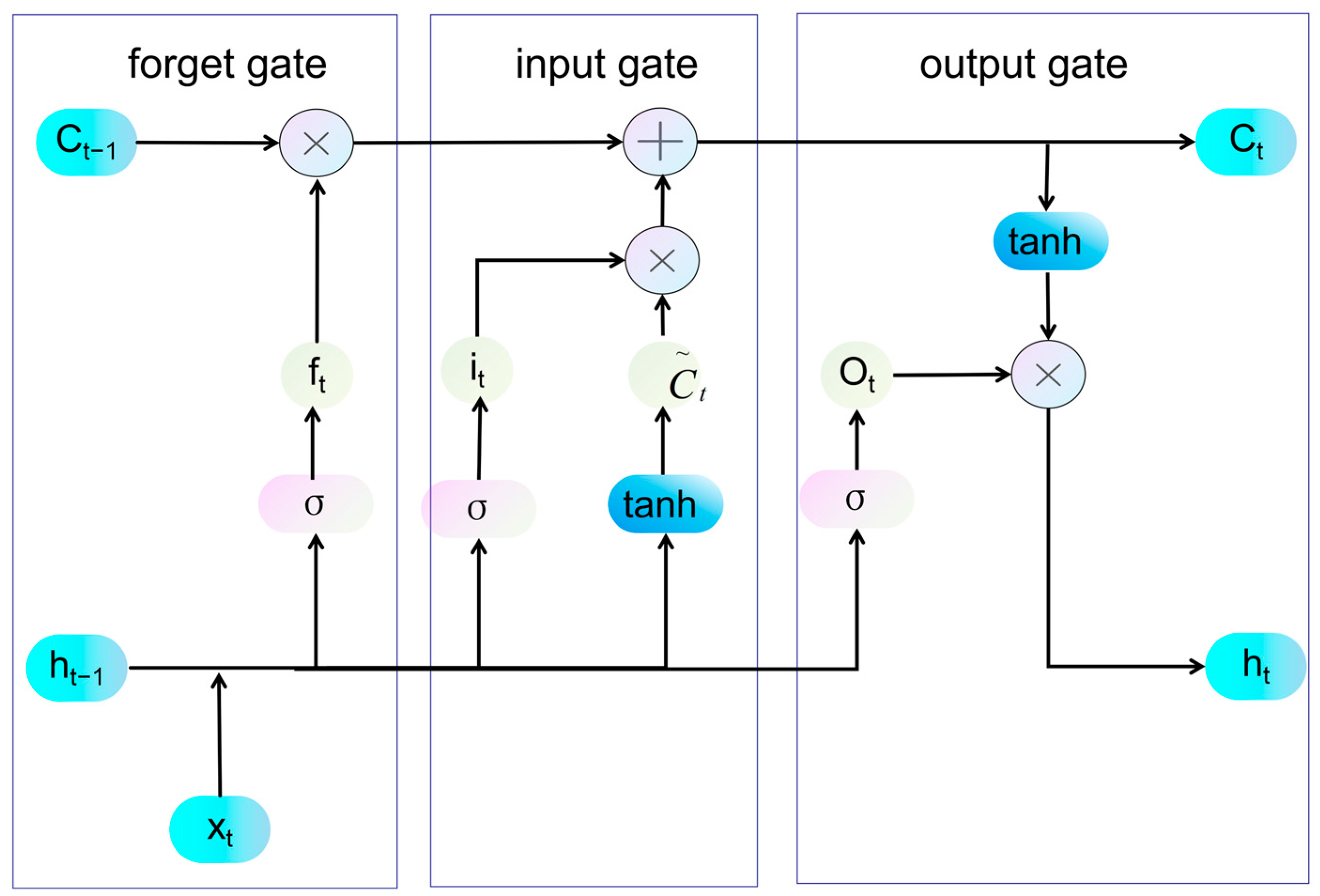
The LSTM structure is as follows in
Figure 1. The core components of LSTM include three gates—the forget gate, the input gate, and the output gate—as well as two types of memory units: the short-term unit and the long-term unit.
Forgetting gate: This component regulates the portion and extent of state information from the long-term memory unit that needs to be disregarded from the previous moment. It also selects the useful information that should be retained after passing through the forgetting gate.
In the formula,
ft decides the information to be forgotten.
ht−1 is the previous step’s short-term memory state, and it is the current step.
Wf (weight matrix) and
bf (bias term) are learnable parameters.
σ is the sigmoid function, outputting a value between 0 and 1, with its expression below.
Input gate: It controls which information from the short-term memory cell of the previous time step and the cell information of the current time step can enter the current memory cell. This effectively prevents irrelevant information from entering the long-term memory cell.
In this context,
it highlights the specific components from both the previous step’s short-term information and the current step’s cell data that contribute to enhancing the memory cell. The weight matrix, denoted as
Wi, along with the bias term
bi, plays a crucial role in refining this pivotal updating process.
Ct* is the candidate vector enhancing information representation. It controls the new information inflow to the current cell
it. The range is from −1 to 1, encompassing all types of information.
Wc is the weight matrix, and
bc is the bias term for updating potential information. The
tanh function produces outputs ranging from −1 to 1, as shown in the expression below.
The long-term memory cell at the current time step combines information from the previous long-term memory cell with new data, forming a comprehensive unit of information.
Ct is a comprehensive information unit that is then passed to the memory cell of the next time step.
Output gate: It regulates the information that can enter the short-term memory cell at the present step. It decides the final output information, serving as the ultimate checkpoint for data.
where
Ot denotes a synthesized selection vector ranging from 0 to 1. Where
Wo denotes a matrix of correlation weights between the synthesized information and the information in the current output short-term memory unit, and
bo denotes the corresponding bias term.
The short-term memory cell is also called the output unit. It is the information unit that is finally output.
It selects the most important part of the current-step information as the output.
There is a weight matrix composed of Wf, Wi, Wc, and Wo, along with a bias term consisting of bf, bi, bc, and bo. All LSTM layers share these parameters. Thus, training an LSTM means adjusting these parameters to fit the specific task.
With its three-gate mechanism, LSTM can create the information before and after the sequence by participating in the calculation across time sequences, thereby effectively processing evaporator tube leakage monitoring parameters characterized by strong temporal dependencies and extracting critical temporal features. Thus, LSTM excels at temporal modeling by capturing temporal features. Its strength resides in detecting fault-related patterns exhibiting time-specific characteristics.
2.2. CNN Theory
The convolutional neural network (CNN) emerged when LeCun utilized the backpropagation (BP) network to develop LeNet-5, which is a classic CNN architecture [
36]. CNNs are regularized feedforward neural networks that leverage convolution operations and pooling to automatically extract hierarchical features from data. They exhibit high fault tolerance and robustness [
31].
CNN’s structure consists of three key parts: the convolutional layer, the pooling layer, and the activation function layer. The convolutional layer is fundamental to the architecture.
Figure 2 shows how the CNN works.
Convolution operation: Essentially, a convolution kernel slides over the input data. It sums up the weighted values to extract local features from the data at each position.
where
i represents the time position, while
j indicates the variable position, with (
m,
n) serving as the row and column indices corresponding to the convolution kernel
k(
m,
n). Where
k(
m,
n) denotes the value of the convolution kernel at the position (
m,
n). The expression
X(
m +
i,
n +
j) indicates that the variable at the position (
i,
j) slides over the convolution kernel
k(
m,
n). Finally,
Y(
i,
j) represents the value at the position (
i,
j) after the convolution calculation has been performed.
Pooling operation: The pooling operation essentially down-samples the input data, which reduces the volume of data while retaining key features. Max-pooling selects the maximum value within the pooling window, emphasizing the most prominent features and making less obvious fault features more distinct. In this study, max-pooling is chosen because the fault features are somewhat similar. This method helps to highlight the less apparent fault characteristics.
Max-pooling uses the size of the (k, k) pooling window. At position (i, j), it finds the maximum value Y(i, j) within the (k, k) window.
The activation function layer includes Sigmoid,
tanh, ReLU, and so on. In this study, we used a ReLU activation function, which is widely used in CNN models with the advantages of fast convergence and simple gradient calculation. The expression of the ReLU function is as follows:
where
f(
xi) denotes that the value of
f(
xi) is
xi when
xi > 0; otherwise, it is 0.
The 1D-CNNs extract features from the variable-space dimension. They use multiple convolutional filters to perform dot-product operations on input data, extracting local information from the current data slice [
37]. Thus, a 1D-CNN effectively extract local spatial features, enabling the processing of high-dimensional monitoring parameters for evaporator tube leakage while achieving dimensionality reduction.
2.3. Attention Mechanism Theory
The attention mechanism was introduced by Ashish Vaswani, Noam Shazeer, Niki Parmar, and others [
38]. It dynamically assigns weights based on the relationships between elements, which helps capture long-range dependencies and extract global features. The attention process determines the importance of information through feature weighting [
39].
For an input sequence
X = {
x1,
x2,
x3 …
xn}, the attention first uses a linear transformation to generate a query vector
Q, a key vector
K, and a value vector
V (
K =
V). The calculations are as follows:
where
WQ,
WK, and
WV are the weight matrices to be learned. In attention, an attention score matrix,
S, is used to represent the degree of relevance of the focused content. Also, it needs to be divided by a dimensional factor
dk, to prevent gradient vanishing and explosion. The calculation formula of
S is as follows:
where
k represents the dimension size. Then, normalize the attention score,
S, to obtain the attention weights. Finally, multiply by
V to get the final output.
S~ represents the result of normalizing S.
The attention mechanism dynamically assigns weights to temporal steps and spatial features, enabling a task-specific information focus. By integrating the global context, it selectively filters irrelevant data while concentrating on salient features during complex data processing. This capability is critical for precise leakage estimation.
2.4. LSTM-CNN–Attention Framework for Leakage Estimation
This paper proposes an LSTM-CNN–attention framework for evaporator tube leakage estimation according to existing methods. The LSTM-CNN–attention’s schematic is in
Figure 3 and
Figure 4. Input data undergoes sliding window preprocessing to enhance temporal fault features per variable. Then, it passes through the LSTM layer to get each variable’s time-based fault features. LSTM outputs are subsequently reshaped for the heterogeneous dual-channel ACNN module, which integrates the following:
- (1)
A 1D-CNN submodule with dual convolutional layers extracting local fault-variable features, followed by max-pooling for feature refinement;
- (2)
An attention mechanism quantifying spatial variable-fault correlations to derive global spatial fault features.
The concatenated outputs from both channels are fed into a fully connected layer aggregating spatiotemporal fault representations, ultimately generating probabilistic fault distribution estimates.
This study uses one framework for two models. Just change the loss function during training, using BCE for fault diagnosis and MSE for fault severity estimation. We use a fault diagnosis model at first, and then a fault severity estimation model for data diagnosed as faulty.
The LSTM-CNN–attention architecture enables robust feature decoupling through multi-modal feature extraction. Specifically, LSTM captures temporal features per variable, while the dual-channel ACNN structure extracts comprehensive spatial features: 1D-CNN acquires localized spatial patterns, and attention derives global spatial characteristics. This explicit functional segregation prevents feature entanglement. Furthermore, architecture achieves precise leakage estimation from high-dimensional inputs via a staged processing mechanism comprising temporal modeling (LSTM), multidimensional spatial feature fusion (ACNN), and nonlinear mapping (FC).
This lightweight deep learning architecture offers distinct advantages: Reduced computational complexity: Compared to transformer structures, it incurs significantly lower computational overhead. Inherent multi-scale adaptability: A key characteristic is its ability to adapt to multi-scale data without requiring explicit scale alignment, offering greater flexibility than multi-head attention mechanisms. Multidimensional feature extraction: Crucially, the architecture facilitates feature extraction across multiple dimensions. This enables the modeling of complex nonlinear relationships, ultimately achieving the accurate prediction of unknown leakage levels.
This architecture also exhibits strong noise resistance when dealing with noisy real-world operating conditions. Its advantages are particularly pronounced in noisy environments for three key reasons. LSTM-based temporal denoising: The LSTM structure inherently performs denoising along the temporal dimension of features. Its temporal smoothing effect preliminarily reduces noise interference over time. The 1D-CNN’s translation invariance: The 1D-CNN possesses translation invariance, which inherently mitigates the impact of noise on local features. Attention-based dynamic reweighting: The attention mechanism dynamically adjusts the weights of the LSTM-processed features (which already have a lower noise impact) based on the global context. Together, these mechanisms form a dual-channel, two-stage noise suppression framework leveraging both LSTM and CNN pathways.
The LSTM gets time features of leakage faults. CNN extracts local spatial features of fault parameters. The attention adjusts weights to obtain global spatial features of fault parameters. It helps LSTM-CNN–attention fully capture spatiotemporal fault features. The proposed framework addresses the critical challenge of evaporator tube leakage quantification through a triple-layer spatiotemporal modeling mechanism that simultaneously captures high-dimensional monitoring parameters’ spatiotemporal features, decouples strongly correlated variables, and establishes complex nonlinear mappings between inputs and leakage fault characteristics. Overall, LSTM-CNN–attention can map effectively. In summary, the LSTM-CNN–attention framework enables the accurate estimation of evaporator tube leakage magnitude by establishing complex nonlinear mappings between high-dimensional variables and leakage quantities through comprehensive spatiotemporal feature extraction.
4. Result and Discussion
The implementation roadmap for diagnosing evaporator tube leaks and estimating leakage using the LSTM-CNN–attention method proposed in this paper is shown in
Figure 11. The roadmap consists of three parts: data acquisition and processing, fault diagnosis, and fault severity estimation. Firstly, the fault simulation test of evaporator tube leakage is carried out to obtain experimental data and data preprocessing. Then the leakage fault diagnosis model is trained using the training set data and validated on the test set. Finally, the fault data on the training set determined by the leakage fault diagnosis model are used as the training set of the leakage estimation model to be trained and validated on the test set.
We planned to conduct experiments using some common fault diagnosis framework as comparisons, including LSTM–attention, CNN–attention, CNN-LSTM–attention. Accurate fault identification is a prerequisite for estimating fault severity. Thus, it is necessary to explore the performance of LSTM-CNN–attention in diagnosing evaporator tube leakage faults. This study utilized four common fault diagnosis frameworks to diagnose and estimate leakage faults. The LSTM method can achieve 98% accuracy in identifying weak faults in micro-turbine blades, showing high accuracy in minor fault recognition [
41]. The CNN can attain over 99% accuracy in identifying crack and shaft-eccentricity faults in a rotor system under different signal-to-noise ratios [
42]. Yang, et al. proposed CNN-LSTM method which shows excellent performance on the TEP and TPFP datasets, and the addition of an adaptive adversarial domain can realize the fault diagnosis of unlabeled data [
43]. The three frameworks were enhanced by incorporating an attention mechanism, resulting in the following variations: LSTM–attention, CNN–attention, and CNN-LSTM–attention [
44,
45,
46]. Consequently, in subsequent comparative investigations, the LSTM–attention, CNN–attention, and CNN-LSTM–attention frameworks-selected as high-performance baselines-are subjected to rigorous comparative analysis against the proposed LSTM-CNN–attention framework.
The hyperparameter settings for LSTM with attention are based on reference [
47], for CNN with attention on reference [
48], and CNN-LSTM with attention on reference [
33]. All these settings also included fine-tuning. The hyperparameter settings of the leakage estimation methods for the proposed LSTM-CNN–attention are shown in
Table 4.
During the experiment, to ensure consistency in the comparison, the hyperparameters of the reference architectures were configured based on the settings used for the proposed LSTM-CNN–attention architecture in this paper. However, to guarantee the optimal performance of each architecture, fine-tuning through hyperparameter optimization was performed for each reference architecture, building upon the baseline settings from this paper (as the hyperparameters for the proposed architecture were themselves the result of optimization). This ensured that the other three architectures were also tested with their respective optimal hyperparameter configurations, thereby validating the superiority of the architecture proposed in this work.
We planned to use this framework to achieve leakage fault diagnosis and estimation in subsequent experiments. Since the methodology sequentially performs leakage fault detection prior to magnitude estimation, the accurate fault diagnosis of evaporator tube leakage constitutes a fundamental prerequisite for precise leakage quantification. We would compare with other methods to explore the ability of the novel LSTM-CNN–attention method in terms of diagnosing evaporation tube leakage faults, estimating leakage, adapting to operating conditions, and resisting noise. The experimental contents included diagnosis and estimation performance under the same operating conditions with different test sets, different operating condition datasets, and different noise levels.
In addition, for the fault leakage estimation experiments in this paper, each experimental group was repeated ten times, and the reported results represent the average value obtained from these repetitions to mitigate the effects of randomness and ensure reliable results.
4.1. Performance of the Model Under Different Test Sets in Operating Condition 2
Accurate leak fault diagnosis is essential for estimating leakage. Given that data distributions change with leakage and gathering data for all levels of severity is challenging in practice, it is important to investigate the diagnostic and predictive ability of the leakage estimation framework for both known and unseen levels of leakage.
The leakage estimation model used the Mean Squared Error (MSE) loss function, and the fault diagnosis model used the Binary Cross-Entropy (BCE) loss function. We chose the operating condition 2 dataset to train these models with its training set and validated them on test sets 1, 2, and 3.
The process of this method for extracting the fault features of supercharged boiler evaporator tubes is shown in
Figure 12 and
Figure 13.
Figure 12 shows fault feature extraction in the fault diagnosis stage.
Figure 13 shows the same in the fault severity estimation stage.
Figure 12 and
Figure 13 visualize the feature extraction process of models trained using the condition 2 dataset, employing heatmaps for representation.
These feature heatmaps provide an indirect interpretation of the feature extraction process and illustrate the deep feature decoupling. The reason why this architecture performs deep feature decoupling can be explained based on
Figure 12 and
Figure 13.
- (1)
Stage 1: Strong Initial Coupling: As shown in the input layer, the multidimensional input variables (with an actual dimensionality of 140; only key strongly coupled parameters are visualized) exhibit highly complex interdependencies across both variable and temporal dimensions, manifesting strong coupling (darker shades indicate stronger coupling).
- (2)
Stage 2: Reduced Temporal Coupling: The LSTM layer demonstrates the model’s capacity for temporal feature decoupling. After processing by the LSTM, the coupling between time windows (stride = 20) is reduced (evident by distinct color variations along the time axis for certain variables), though significant coupling among variables persists.
- (3)
Stage 3: Reduced Local Spatial Coupling and Reduced Global Spatial Coupling: The Max Pooling Layer (following CNN operations) reveals local spatial feature decoupling. The CNN layer enhances distinguishability between local variables, leading to clearer feature separation within local regions. The attention mechanism performs global feature selection, reducing coupling among critical features. Key features exhibit distinct separation across the global variable dimension.
- (4)
Stage 4: Evident Spatiotemporal Feature Decoupling: Decoupled features from the CNN and self-attention mechanisms are concatenated. Subsequent processing through fully connected layers enables effective fault classification and leakage quantification, as evidenced by the well-separated outputs in the final layer.
Collectively,
Figure 12 and
Figure 13 indirectly illustrate the framework’s capability for deep feature decoupling.
4.1.1. Diagnostic and Estimation Results for Test Set 1
Table 5 shows the results of the average diagnostic accuracy (ADA), average estimation accuracy (AEA), and maximum relative error of estimation (MREE) of the model on test set 1.
LSTM-CNN–attention has the highest ADA for supercharged boiler leaks at 99.33% from
Table 5. Its AEA is only 0.47% lower than CNN–attention, with an MREE of just 4.96%. The other three frameworks also show a certain accuracy in diagnosing and estimating fault severity. But as fault diagnosis is the prerequisite, LSTM-CNN–attention performs best on test set 1 for diagnosing and estimating the known leakages.
Figure 14a displays the estimated leakage from the evaporator tube based on test set 1.
Figure 14b illustrates the relative error results for the leakage estimations at various moments on test set 1. The dotted line indicates a relative error threshold of 20%. Typically, the relative error for severity estimations should be below this 20% limit.
The LSTM-CNN–attention framework is the most accurate and stable option for estimating known leakages.
Figure 14a shows that the estimated leakages from the LSTM-CNN–attention, CNN–attention, and CNN-LSTM–attention models are closer to the true value of 0.09 in terms of both range and trend.
Figure 14b indicates that the LSTM-CNN–attention model can maintain a relative estimation error within 5% for more stable leakage estimations.
Overall, LSTM-CNN–attention is the best on test set 1 for diagnosing and is the most accurate and stable method for known leakage estimation.
4.1.2. Diagnostic and Estimation Results for Test Set 2
Table 6 shows the results of the average diagnostic accuracy (ADA), average estimation accuracy (AEA), and maximum relative error of estimation (MREE) of the model on test set 2.
Figure 15a displays the estimated leakage from the evaporator tube based on test set 2.
Figure 15b illustrates the relative error results for the leakage estimations at various moments on test set 2.
The LSTM-CNN–attention method shows the highest accuracy in diagnosing and estimating unseen leakage on test set 2. As can be seen from
Table 6, this method achieves an impressive ADA of 99.93%. Additionally, it records the highest AEA at 90.28%, with an MREE of 18.89%.
As depicted in
Figure 15a, the distributions of the estimated values of LSTM-CNN–attention, LSTM–attention, and CNN–attention are all close to the actual leakage. However, some of the estimated values of CNN–attention deviate significantly. In
Figure 15b, only the relative estimation error of LSTM-CNN–attention can consistently remain within 20%, maintaining a stable estimation ability. Therefore, the LSTM-CNN–attention framework shows the best performance in estimating the unseen evaporator tube leakage on test set 2.
Overall, LSTM-CNN–attention is the best framework on test set 2 and the most accurate and stable method for the unseen leakage estimation.
4.1.3. Diagnostic and Estimation Results for Test Set 3
Table 7 shows the results of the average diagnostic accuracy (ADA), average estimation accuracy (AEA), and maximum relative error of estimation (MREE) of the model on test set 3.
Figure 16a displays the estimated leakage from the evaporator tube based on test set 3.
Figure 16b illustrates the relative error results for the leakage estimations at various moments on test set 3.
Table 7 shows LSTM-CNN–attention has the highest ADA for supercharged boiler leaks, reaching 99.56%. Its AEA for leakage is also the highest, at 94.74%, with the lowest MREE of 7.29%. On test set 3, LSTM-CNN–attention is the most accurate in diagnosing and estimating the unseen leakage.
Figure 16a shows that the estimated values of LSTM-CNN–attention and LSTM–attention are closer to the real leakage.
Figure 16b shows that their relative estimation errors are below 20%, so they are more stable in estimating leakage.
Overall, LSTM-CNN–attention is the best framework on test set 3. LSTM-CNN–attention and LSTM–attention are the most accurate and stable methods for the unseen leakage estimation.
Under condition 2, the LSTM-CNN–attention framework demonstrates the precise identification of evaporator tube leakage and accurate magnitude estimation, achieving superior accuracy over three existing deep learning architectures. Its high fault diagnosis accuracy confirms robust spatiotemporal feature extraction capabilities, while precise leakage quantification with a minimal estimation error and a maximum deviation error validates its effective complex nonlinear mapping from high-dimensional inputs to leakage magnitude. However, given its condition-specific applicability, subsequent sections investigate the framework’s performance across diverse operational scenarios.
4.2. The Cross-Conditional Performance Evaluation of the Frameworks
We need to examine the performance of the frameworks under different operating conditions. Given the significant differences in data distribution across these conditions and considering that diverse scenarios can arise during the operation of a supercharged boiler, the model must be capable of handling datasets from different situations.
The fault diagnosis and fault severity models use the same parameter settings as in the previous experiments. We trained the two models using the training sets from operating conditions 1 and 3. We evaluated the model performance using the data division method from test set 2 after training as the experiment for operating condition 2 was completed in experiment 2.
4.2.1. Estimation Results for the Dataset of Operating Condition 1
Table 8 shows the results of the average diagnostic accuracy (ADA), average estimation accuracy (AEA), and maximum relative error of estimation (MREE) of the model on operating condition 1.
Figure 17a displays the estimated leakage from the evaporator tube based on operating condition 1.
Figure 17b illustrates the relative error results for the leakage estimations at various moments on operating condition 1.
Table 8 indicates that under operating condition 1, the ADAs of the four frameworks can all reach over 99%, and the AEAs of all of them can reach over 90%. Among them, LSTM–attention has the highest AEA. Its ADA is only 0.17% lower than that of LSTM-CNN–attention, and it has an MREE of 4.92%. In addition, LSTM-CNN–attention also has the highest ADA, the second-highest AEA, with 96.62%, and the second-lowest MREE of the estimation, with 9.48%. So, LSTM–attention has the best performance, and LSTM-CNN–attention has the second-best performance on operating condition 1.
As can be seen from
Figure 17a, the estimated value distributions of LSTM–attention, CNN-LSTM–attention, and LSTM-CNN–attention are all close to the actual leakage volume.
Figure 17b shows that the relative estimation errors of the four methods can all be controlled within 20%. The relative estimation errors of LSTM–attention and LSTM-CNN–attention remain within 10%. This indicates that under operating condition 1, LSTM–attention has the highest accuracy in diagnosing and estimating the leakage of the supercharged boiler evaporator tube.
Overall, LSTM–attention is an accurate framework for diagnosis and estimation of leakage and is the most stable framework for known leakage estimation on operating condition 1. In addition, LSTM-CNN–attention also has a very high accuracy for diagnosis and estimation of leakage, and a very stable method for unseen leakage estimation on operating condition 1.
4.2.2. Diagnostic and Estimation Results on Test Set 2 for the Dataset of Operating Condition 3
Table 9 shows the results of the average diagnostic accuracy (ADA), average estimation accuracy (AEA), and maximum relative error of estimation (MREE) of the model on operating condition 3.
Figure 18a displays the estimated leakage from the evaporator tube based on operating condition 3.
Figure 18b illustrates the relative error results for the leakage estimations at various moments on operating condition 3.
Table 9 indicates that under operating condition 3, all four methods achieve an ADA over 99% and an AEA above 85%. LSTM-CNN–attention tops the group, with an ADA of 99.99% and AEA of 93.89%, along with the smallest MREE of 11.73%.
LSTM-CNN–attention is the most accurate and stable method for unseen leakage estimation on operating condition 2.
Figure 18a shows that the estimated value distributions of LSTM–attention, CNN–attention, and LSTM-CNN–attention are closer to the actual leakage volume.
Figure 18b reveals that relative estimation errors of the four methods are within 20%, except for some of those from CNN-LSTM–attention. LSTM-CNN–attention has a more stable estimation with a relatively lower error distribution. Hence, LSTM-CNN–attention is more accurate and stable in diagnosing and estimating evaporator tube leakage under operating condition 3.
Both LSTM-CNN–attention and LSTM–attention, whose results are very close on operating conditions 1, 2, and 3, show excellent adaptability to different boiler operating conditions regarding evaporator tube leakage. Since ship boiler operating conditions vary during actual voyages, such adaptability is crucial. Analyzing the results, although both LSTM-CNN–attention and LSTM–attention methods perform well in operating condition adaptability, LSTM-CNN–attention has a better performance on predictive capability. Therefore, LSTM-CNN–attention, with a better predictive capability and operating condition adaptability, is more suitable for diagnosing boiler evaporator tube leakage and estimating leakage.
4.3. The Impact of Noise on the Models
We need to explore the impact of noise on the models. As the dataset employed in this study is sourced from simulation experiments, the associated data noise is minimal. Nevertheless, the data acquired by sensors of supercharged boilers typically encompasses a certain level of noise in the actual motion of boilers. Consequently, the model needs to exhibit robust noise resistance characteristics.
In marine boilers, the noise level varies among different hull models. Commonly, the noise picked up by boiler sensors is Gaussian white noise. The formula for calculating the signal-to-noise ratio is as follows:
In this context, SNR stands for the signal-to-noise ratio. Notably, a lower SNR value corresponds to a higher noise power, where Ps and Pn signify the signal power and noise power, respectively. For this experiment, a series of SNR values, spanning from −7 to a noise-free condition, was carefully set up. Conventionally, during ship navigation, the SNR of the signals received by supercharged boiler sensors typically ranges from −3 dB to 3 dB. Specifically, the dataset under operating condition 2 was chosen, and test set 2 was employed to evaluate how noise influences the model. To quantify this impact, three main parameters were utilized: ADA, AEA, and the MREE of estimation.
Figure 19 visually shows the change in diagnosis average accuracy (ADA) with SNR.
Figure 20 visually shows the change in estimation average accuracy (AEA) with SNR.
Figure 21 visually shows the change of maximum relative error of estimation (MREE) with SNR.
LSTM-CNN–attention has the strongest noise immunity in the diagnosis of evaporator tube leak faults. As illustrated in
Figure 19, an increase in noise power led to a decline in the SNR, causing the ADA of the four methods to trend downward. However, even at an SNR of −7 dB, the LSTM-CNN–attention method sustains an accuracy of 90%, outperforming the other three methods.
LSTM-CNN–attention has the strongest noise immunity in the estimation of evaporator tube leakage.
Figure 20 shows that LSTM-CNN–attention not only achieves a relatively high accuracy but also shows the least sensitivity to noise for estimating fault severity. Although CNN-LSTM–attention had the smallest impact of noise, its ADA consistently remained below 80%. Although the other three methods experience a reduction in accuracy due to noise, they demonstrate higher accuracies in noise-free conditions. When the SNR exceeded −4 dB, LSTM-CNN–attention can maintain an AEA of over 80%.
LSTM-CNN–attention possesses the strongest noise immunity in real-world noise, with the least extreme peak estimation error. As depicted in
Figure 21, when the SNR is greater than −4 dB, LSTM-CNN–attention exhibits the smallest MREE, which remains at a relatively low level. When the SNR dropped below −4 dB, CNN-LSTM–attention attained the smallest MREE. But an SNR of −4 dB represents intense noise interference in actual motion. Typically, during the actual operation of a marine vessel, the SNR of the supercharged boiler ranges from −3 dB to 4 dB.
The LSTM-CNN–attention framework showcases robust noise resistance ability for the leak fault diagnosis and leakage estimation of the boiler evaporator tube, rendering it highly applicable to real-world engineering scenarios. A comprehensive analysis of the experimental results reveals that, while ensuring high diagnostic and estimation accuracies, LSTM-CNN attention is less affected by noise. It can endure an extreme SNR of approximately −4 dB, maintaining an average diagnostic accuracy above 90% and an average estimation accuracy above 80%.
Although LSTM–attention demonstrates commendable adaptability to diverse operating conditions, it lags in terms of its predictive capability and noise resistance. Compared to the three alternative frameworks, the LSTM-CNN–attention architecture demonstrates a superior predictive capability, exceptional operational adaptability, and optimal noise immunity, establishing itself as the preeminent framework for evaporator tube leakage magnitude estimation.


