Article

Economic Growth and Energy Consumption in Thailand: Evidence from the Energy Kuznets Curve Using Provincial-Level Data

by
Thanakhom Srisaringkarn
and
Kentaka Aruga
*
Graduate School of Humanities and Social Sciences, Saitama University, 255 Shimo-Okubo, Sakura-ku, Saitama 338-8570, Japan
*
Author to whom correspondence should be addressed.
Energies 2025, 18(15), 3980; https://doi.org/10.3390/en18153980
Submission received: 23 May 2025 / Revised: 20 July 2025 / Accepted: 22 July 2025 / Published: 25 July 2025
(This article belongs to the Special Issue Environmental Sustainability and Energy Economy)

Abstract

This study investigates the relationship between economic growth and energy consumption using the Energy Kuznets Curve (EKC) framework. Spatial econometric models, including the Spatial Panel Lag Model and the Spatial Dynamic Panel Lag IV Model, are employed to capture both spatial and dynamic effects. The results indicate that energy consumption in Thailand is spatially clustered, with energy use tending to spill over into neighboring provinces and concentrating in specific regions. Key factors that positively influence energy consumption include gross provincial product (GPP) per capita, population density, and road density. Regions characterized by favorable climates, sufficient infrastructure, and high levels of economic activity exhibit higher per capita energy consumption. The EKC analysis reveals a U-shape relationship between GPP per capita and energy consumption in the BKK&VIC, CE, EA, WE, and NE regions. As many regions continue to experience rising energy consumption, the findings underscore the importance of Thailand adopting more efficient energy usage strategies in tandem with its economic development.

1. Introduction

Thailand is a developing country whose manufacturing sector relies heavily on energy. From Figure 1, Figure 2 and Figure 3 it can be observed that within the Association of Southeast Asian Nations (ASEAN), Thailand has the highest electricity consumption per capita and the highest electricity production from oil sources among all ASEAN countries, excluding Malaysia, Brunei, and Singapore, which have larger economies than Thailand. In contrast, Thailand has the lowest share of combustible renewables and waste compared to its neighboring developing countries with smaller economies, such as Myanmar, Cambodia, and Lao PDR. Thailand’s economic expansion has been driven by industrialization, informatization, urbanization, and agricultural modernization, all of which rely heavily on energy consumption. According to the Office of the National Economic and Social Development Board, Thailand’s electricity consumption grew at an average annual rate of 3.5% between 1990 and 2019, while the economy expanded at an average annual rate of 3.7% over the same period. This suggests a potential correlation between electricity consumption and economic development in Thailand.
Domestic electricity demand in Thailand, which fluctuates in line with economic activity (Figure 4), exhibits distinct patterns across various economic sectors. Over the past 10 years (average from 2013 to 2023), electricity consumption was distributed as follows: the industrial sector accounted for 46.7%, the household sector for 25.1%, the business sector for 24.0%, and other sectors for 4.2% of the country’s total electricity consumption. Within the industrial sector, the highest electricity-consuming industries include food processing, steel and basic metals, rubber and rubber products, electronics, plastics, and textiles. In the business sector, the largest electricity users are primarily tourism-related services, including hotels, restaurants, nightclubs, apartments, guesthouses, department stores, and retail and wholesale establishments [4].
As illustrated in Figure 5, the trends in energy consumption and economic growth from 2015 to 2022 were closely correlated. Electricity can be generated from both renewable and non-renewable energy sources (Figure 6a,b). When electricity is generated from renewable sources, it can significantly reduce greenhouse gas emissions. Conversely, electricity generation based on non-renewable sources has been found to have a negative impact on environmental quality, particularly when consumption increases [6]. Figure 6a,b show that more than 85% of electricity generation in 2015 and 71% in 2022 came from non-renewable sources. This indicates that electricity generation in Thailand still largely relies on traditional energy sources, which are associated with high emissions during the production process and are gradually being depleted. This highlights the unsustainability of Thailand’s current electricity consumption patterns.
Thailand consumes a high amount of energy, with relatively limited domestic energy resources compared to its neighboring countries. Thailand is the largest energy consumer in ASEAN and imports significant amounts of natural gas for electricity generation, ranking second only to Singapore, which has a larger economy. As a result, Thailand is the most reliant on imported natural gas among the ASEAN countries [9]. The Electricity Generating Authority of Thailand (EGAT), the state-owned electricity producer, accounts for 40% of the country’s total electricity generation capacity. To reduce dependency and spread the risk associated with relying heavily on natural gas, particularly from neighboring countries, the Thai government has developed a plan to diversify the energy mix. This includes reducing the current 70% reliance on natural gas by increasing the share of coal in electricity production while incorporating clean coal technologies to mitigate environmental impacts [10]. It can be seen that if energy demand continues to increase in the future, Thailand may face challenges related to energy security and become increasingly dependent on energy imports from neighboring countries. Moreover, the current electricity generation technologies used in Thailand significantly contribute to environmental pollution and are unsustainable in the long term [10]. Therefore, this study applies the Energy Kuznets Curve (EKC) theory to examine the relationship between economic growth and energy consumption, to understand how energy consumption in Thailand may evolve as the economy grows. The goal is to support effective energy planning that aligns with the country’s energy consumption trends. In addition, the study aims to provide policy recommendations that align with the Thai government’s target of increasing the share of renewable energy, such as solar, wind, and biomass, to 15–20% by 2036 [10].
Gross regional product (GRP), GRP per capita, energy consumption, and energy consumption per capita by region in Thailand are presented in Table 1. Figure 7 shows the boundaries of Thailand’s 77 provinces. The region with the highest GRP and average energy consumption per capita is Bangkok and vicinity (BKK&VIC), followed by the northeastern region (NE) and the southern region (SO). The remaining regions, such as the northern region (NO), exhibit the lowest levels of economic activity [11]. However, Bangkok and vicinity (BKK&VIC), the eastern region (EA), the central region (CE), and the western region (WE) are combined in this study, as they are classified as high-economic-growth pole regions in central Thailand. In this study, we use provincial-level data from all 77 provinces of Thailand as representative data points and categorize them into the four areas mentioned above to analyze the impact of economic growth on energy consumption based on the EKC theory. This regional approach aims to provide more comprehensive and tailored policy recommendations compared to a whole-region analysis alone, taking into account variations in economic structure, geography, and environmental conditions across different regions.
Several studies have investigated the impact of economic growth on energy consumption and air pollution using various methodologies, such as Autoregressive Distributed Lag (ARDL) cointegration analysis, Fully Modified Ordinary Least Squares (FMOLS), and Dynamic Ordinary Least Squares (DOLS), predominantly relying on provincial-level, ground-based data in Thailand [6,14,15,16,17,18]. Additionally, Maneejuk et al. [19] proposed the Simultaneous Smooth Transition Kink Equations (SKE) model, in which each regression parameter can exist in two different regimes, lower and upper, to examine the presence of the Kuznets Curve in Thailand’s economy over the past two decades. A research gap is identified through the review of previous studies, presenting an opportunity to extend the existing literature. This study aims to fill that gap by utilizing provincial-level data in Thailand, combined with environmental data from satellite observations, to offer a more localized and specific analysis of the impacts occurring within the country. Moreover, this study employs the Spatial Dynamic Panel IV Model (SDPD IV), which captures dynamic effects over time and accounts for spatial spillover effects across regions in Thailand.
Therefore, this study examines how energy consumption and economic growth in Thailand and its regions are likely to evolve in the short and long term under continued economic growth. It also seeks to assess whether energy consumption will become more sustainable. Additionally, the study investigates the characteristics of energy consumption concentration in Thailand and analyzes the relationship patterns between energy consumption and its influencing factors. The ultimate goal is to enhance the understanding of energy consumption patterns associated with economic growth in Thailand and to support the formulation of appropriate, region-specific energy policies in the future.
The following section presents the theoretical framework of the study. The second section outlines the analytical methods used, while the third section presents the empirical results. The fourth section offers a discussion of the findings. Finally, the last section provides the conclusions and policy implications.

1.1. Energy Kuznets Curve Theory

The Kuznets Curve, introduced by Kuznets [20], was developed to explore the relationship between economic growth and income inequality. Over the past five decades, Grossman and Krueger [21] extended this concept to develop the Environmental Kuznets Curve. This theory hypothesizes a relationship between various indicators of environmental degradation and per capita income. In the early stages of economic growth, pollution emissions increase, and environmental quality deteriorates. However, beyond a certain level of per capita income (which varies depending on the indicator), this trend reverses, and further economic growth leads to environmental improvement. This implies that environmental impacts or emissions per capita follow an inverted U-shape relationship with per capita income [21,22,23,24]. This study applies the Energy Kuznets Curve (EKC) theory, which is conceptually similar to the Environmental Kuznets Curve. However, the EKC focuses specifically on the relationship between economic growth and energy consumption, as discussed by Suri and Chapman [25]. Understanding the relationship between economic growth and energy consumption, as outlined in the EKC theory, will help to identify the direction of energy consumption as the economy continues to expand. This insight can guide the planning and management of sustainable and efficient energy use in the future. Although various empirical studies have confirmed the EKC hypothesis in some instances, it is not universally applicable across all types of environmental degradation, income groups, or national contexts [26]. Throughout this paper, the EKC theory generally refers to the Energy Kuznets Curve.
Table 2 summarizes findings from various studies examining the impact of economic growth on energy consumption and air pollution. Some studies have identified different EKC and Environmental Kuznets Curve patterns, including monotonic increases, inverted U-shape, U-shape, and N-shape. This study incorporates variables based on the research findings summarized in Table 2 to analyze the relationship between economic growth and energy consumption in each region of Thailand. The aim is to identify EKC patterns that can inform the development of important policy recommendations for the country. This study adopts an alternative approach, utilizing provincial-level and satellite data to analyze the EKC pattern in each region, in contrast to previous studies that relied on country-level data and ground-based measurements. As a result, this study provides more localized insights into Thailand’s energy consumption and offers more precise implications for national energy policy.

1.2. Socioeconomic Factors Affecting Energy Consumption

In addition to the main variables commonly used to explore the EKC theory, several other studies have examined the relationship between energy consumption and environmental impact. For example, Zhang et al. [48] tested the EKC hypothesis for Pakistan by analyzing the significance of renewable and non-renewable energy consumption. Their results strongly support the EKC hypothesis in Pakistan, showing that renewable energy plays a dominant role in reducing carbon dioxide emissions. In contrast, non-renewable energy consumption is the primary contributor to increased emissions. Marques et al. [49] analyzed the relationship between economic growth and CO2 emissions in Australia, using annual data from 1965 to 2016, with a focus on fossil fuel (oil and coal) and renewable energy consumption. Their results support the EKC hypothesis, suggesting that Australia is experiencing increased relative decoupling, which indicates that economic growth continues to drive CO2 emissions and environmental degradation. Mahmood [50] examined the asymmetric environmental effects of different energy sources and tested the EKC hypothesis in the Gulf Cooperation Council (GCC) region from 1975 to 2019. The findings show that CO2 emissions resulting from increased natural gas consumption are less severe than those from oil consumption. As a result, the study recommends that GCC countries shift from oil to natural gas to reduce overall CO2 emissions. Pablo-Romero and De Jesús [32] investigated the relationship between economic growth and energy consumption using the hypothesis postulated for the EKC, which assumes an inverted-U shape relationship between income and energy consumption, for 22 Latin American and Caribbean countries for the period 1990–2011. The hypothesis postulated for the EKC is not supported for the region. Aruga [43] investigated the EKC hypothesis among the 19 countries in the Asia–Pacific region. The study also tests the EKC hypothesis for low-, middle-, and high-income groups within the region. The test results of both models suggest that the EKC hypothesis holds for the whole Asia–Pacific region. However, the test performed on the three different income groups revealed that the hypothesis only holds for the high-income group. The hypothesis was not apparent for the low- and middle-income groups.
Based on the literature review, this study utilizes variables such as energy consumption per capita, GPP per capita, and population density, which are commonly used to examine the relationship between economic growth and energy consumption. However, unlike previous studies, this research introduces additional control variables, such as road density, and instrumental variables, including nighttime land surface temperature, rainfall, and wind speed, all derived from satellite data at the provincial level in Thailand. Satellite data offer high spatial resolution and low-cost accessibility, making them a valuable alternative for developing countries that lack comprehensive environmental data collection across all provinces.

2. Materials and Methods

The overview of the research workflow for this study includes all key steps, beginning with the background and a literature review based on the Environmental Kuznets Curve theory, as discussed by Grossman and Krueger [21] and Suri and Chapman [25]. This theory serves as the main framework for this study. Next, the data and methodology are established by identifying stationary variables, followed by conducting spatial analysis tests to determine the most appropriate spatial econometric model.
In this context, we use spatial econometrics to address spatial interaction (spatial autocorrelation) and spatial structure (spatial heterogeneity) in regression models for panel data. This method incorporates both spatial (geographical) and time dimensions. The focus on location and spatial interaction has recently gained prominence not only in applied but also in theoretical econometrics, particularly in models such as the Spatial Lag Model (SLM), the Spatial Error Model (SEM), and the Spatial Dynamic Panel Model (SDPD) [51]. After identifying stationary variables, serial correlation, and multicollinearity problems, we conduct a Spatial Correlation Test (LM-test) to determine whether the SLM or SEM model is more appropriate. Additionally, the Hausman test is used to decide whether a fixed-effects or random-effects model should be employed. Once the appropriate model type (SLM or SEM) is identified, it is integrated into the Spatial Dynamic Panel Model (SDPD) framework for estimating the variables. This study adopts the Spatial Dynamic Panel Instrumental Variables Model (SDPD IV), which provides consistent and accurate estimates, particularly when the sample size is large. The selection of instrumental variables is validated using the two-stage least squares (2SLS) method. This approach ultimately aims to identify the most appropriate model for estimating the relationships among variables. Furthermore, a Generalized Additive Model (GAM) analysis is employed as a supplementary method to enhance policy-relevant insights, similar to the role of hot spot analysis. Finally, all analytical results are synthesized to provide policy recommendations. These steps are illustrated in Figure 8.
Based on previous studies [17,35,36,37,40,41,43], Equation (1) illustrates the functional relationship between energy consumption per capita (Energycons_pc) and the variables grounded in the EKC theory, as identified through the literature review summarized in Table 2. In addition, this study incorporates a road density variable derived from satellite-based data to generate meaningful insights.

2.1. Model

E n e r g y c o n s p c   =   ( G P P p c ,   G P P p c 2 , P o p _ d e n s ,   R o a d d e n s )
All the variables used in the analysis are presented in Table 3. In this study, energy consumption per capita (Energycons_pc) is the dependent variable. The independent variables include gross provincial product per capita (GPPpc), population density (Pop_dens), and road density (Roaddens). Land surface temperature at night (Landtemp_night), rainfall (Rainfall), and wind speed (Windspeed) are used as instrumental variables. Gross provincial product per capita squared (GPPpc2) is included to capture the nonlinear relationship between GPPpc2 and energy consumption per capita, which may take the form of a turning point, typically represented by an inverted U-shape or U-shape curve. Three underlying effects explain the inverted U-shape: the scale effect (as the economy grows, energy consumption increases, leading to more pollution), the composition effect (a structural shift from low-tech to high-tech industries as the country develops), and the technical effect (benefits from high-tech and cleaner technologies following industrial transformation, resulting in reduced pollution during later stages of economic growth). Economies that exhibit all three effects are expected to follow the EKC pattern, which is characterized by an inverted U-shape [26].
The results of the panel unit root tests used to determine whether the variables in the model are stationary are shown in Appendix A, Table A1. If the variables are not stationary, it can lead to spurious regression results. The Levin, Lin, and Chu (LLC) test and the Im, Pesaran, and Shin (IPS) test were applied. The results indicate that most variables are stationary at the level, i.e., I(0). However, some variables, such as Pop_dens of the northeastern (NE) region and Landtemp_night of the southern (SO) region, are stationary at the first difference, i.e., I(1), after differencing. Additionally, the Breusch–Godfrey test was conducted to identify the presence of serial correlation, and variance inflation factors (VIFs) were calculated to detect multicollinearity issues (Appendix B, Table A2).

2.2. Moran’s I Statistical Test

Developed by Moran [65], Moran’s I test is a statistical tool used to assess spatial autocorrelation in regression residuals by measuring their correlation with neighboring observations. It is used to confirm the presence of spatial correlation in a dataset. If the null hypothesis of no spatial autocorrelation is rejected, the OLS estimates are considered misspecified due to the omission of spatial relationships. Equation (2) presents the mathematical formulation of Moran’s I test.
I = [ i j w i , j x i x ¯ ( x j x ¯ ) ] i j w i , j ( x i x ¯ ) 2
Here, Wi,j is the spatial weight matrix, and x i and x j are the values of the variable of interest in the respective areas. A statistically significant Moran’s I result confirms the presence of spatial effects.
As shown in Table 4, the K-nearest neighbors (K-NN) method was used to construct the spatial weight matrix as K-NN can generate a weight matrix regardless of absolute distance. This approach is particularly suitable for provinces like Phuket, which, being an island, does not share borders with any other province in Thailand. The Moran’s I values are close to 1 and statistically significant at the 1% level (p-value < 0.001), indicating strong spatial clustering of energy consumption. Given this spatial dependence, the study applies spatial econometric methods, specifically the Spatial Panel Lag Model (SLM) and the Spatial Dynamic Panel Lag Model (SDPD), to analyze the spatial diffusion and effects of energy consumption across regions.

2.3. High/Low Clustering (G*) (Hot Spot Analysis)

High/low clustering (Getis-Ord General G or G* test), also known as “hot spot analysis”, was developed by Getis and Ord [66]. This test is a tool for measuring the value of some variables that cluster in certain areas. The null hypothesis states that there is no spatial clustering of feature values. This method can identify spatial cluster patterns in each region, thereby improving the interpretability of the results and facilitating policy implications. Equation (3) represents the mathematical representation of high/low clustering:
G = i   =   1 n j   =   1 n w i , j x i x j i   =   1 n j   =   1 n x i x j ,   j i
where x i   and x j are the attribute values of variables in the interest area i and j, respectively, and wi,j is the spatial weight matrix. When the test shows that the null hypothesis is rejected, it confirms the concentration of value and clustering.

2.4. LM Test for Spatial Dependence (LM-Lag, LM-Error), LM Test for Random Effects, LM Test for Serial Correlation

We conducted the LM test for spatial dependence to determine the most appropriate model for the dataset and to assess whether a lag or error model is more suitable. Based on the results, we can then select the specific model type to be used throughout the study.
Table 5 shows that Moran’s I statistic is 2.554, with a corresponding p-value of 0.01, which is less than 0.05. This indicates that the sample data exhibits spatial correlation. Although, the LM-Error and LM-Lag tests are insignificant. However, the results of Moran’s I statistical test remain statistically significant, indicating that it is appropriate to apply a spatial econometric model to capture the spillover effects of variables influencing neighboring provinces. The choice of a spatial econometric model depends on the form of spatial dependence between units and the type of spatial interaction effect that is present. Although taking the Dynamic Spatial Durbin model (DSDM) as a benchmark model is theoretically reasonable, further tests should be conducted to confirm this. We initially estimated several spatial econometric models to identify the most suitable one for this study, based on Equation (5), using the AIC (Akaike information criterion) and BIC (Bayesian information criterion) values as primary criteria for model comparison. The results show that the Spatial Lag Model (SLM) has the lowest AIC and BIC values (AIC: −1840.59 and BIC: −1796.36), while the Spatial Error Model (SEM) has an AIC of −1823.54 and BIC of −1779.31, and the Spatial Durbin Model (SDM) has an AIC of −1830.87 and BIC of −1751.26. Therefore, the SLM method is employed to estimate the results and address the research questions of this study. The Spatial Lag Model (SLM) captures substantive spatial dependence by directly incorporating spatial interaction into the model rather than merely correcting for the potentially biasing effects of spatial autocorrelation that may arise from the use of spatial data or nonlinear parametric restrictions. This makes the SLM approach more suitable than the SEM or other spatial econometric models (e.g., SDM and SDEM) [51,67]. Additionally, the Hausman test rejects the null hypothesis of the random-effects model, indicating that the fixed-effects model is more appropriate for these datasets.

2.5. Spatial Panel Lag Model (SLM)

After conducting the LM test for spatial dependence, we apply the Spatial Panel Lag Model (SLM) to verify the presence of spatial dependence or the similarity of observations in neighboring areas. This model captures the spatial effects of surrounding regions by including a spatially lagged dependent variable. Moreover, the SLM serves as the baseline model for comparison with the Spatial Dynamic Panel Lag Model (SDPD IV) to determine which provides the most accurate estimation results. The conclusion will be drawn based on the model that yields the most reliable outcomes. The mathematical expression of the model is as follows:
y i = ρ W i , j y j + x i β + u i
where ρ W i , j y j is the vector of the dependent variable y j multiplied by the spatial weight matrix W i , j , which represents another spatially lagged dependent variable; x i is the vector of explanatory variables; and β is a vector of parameters. Using this model our EKC model is analyzed using Equation (5):
L n E n e r g y c o n s _ p c i , t = a + ρ W L n E n e r g y c o n s _ p c i , t + β 1 L n G P P p c i , t + β 2 L n G P P p c 2 i , t + β 3 L n P o p _ d e n s i , t + β 4 L n L a n d t e m p _ n i g h t i , t + β 5 L n R a i n f a l l i , t + β 6 L n W i n d s p e e d i , t + β 7 L n R a o d d e n s i , t + β 8 C O V I D i , t + μ i + λ i + ε i , t
In this equation, ρ is the spatial autoregressive coefficient indicating the spatial spillover effect of energy consumption per capita ( E n e r g y c o n s _ p c ) , and W L n E n e r g y c o n s _ p c i , t is the spatially lagged dependent variable of energy consumption per capita ( E n e r g y c o n s _ p c ) .
We aim to utilize the full SLM model as a benchmark for comparison with the SDPD IV model, determining which provides more accurate estimation results based on the lowest root mean square error (RMSE) and mean absolute error (MAE) values.

2.6. Spatial Dynamic Panel Lag Instrumental Variables Fixed-Effects Model (SDPD IV)

Regional energy consumption per capita is influenced not only by local factors but also by the region’s past energy consumption and by the energy consumption per capita in other regions during both the current and previous periods. This study adopts the Spatial Dynamic Panel Lag IV Model [68,69] to analyze the impact of energy consumption per capita on economic growth in Thailand, expressed as follows:
y i , t = φ j   =   1 n w i , j y j , t + ρ y i , t 1 + x i , t β + γ y , i f y , t + ε i , t
where y i , t denotes the observation on the dependent variable for individual unit i at time period t, and x i , t is a k × 1 vector of covariates with slope coefficients β . The lagged dependent variable y i , t 1 captures dynamic or temporal effects due to state dependence. The error term of the model is composite: f y , t and γ y , i denote ry × 1 vectors of latent factors and factor loadings, respectively, and ε i , t is an idiosyncratic error. The “spatial-lag” variable w i , j y j , t is a weighted average of the outcome variable in the neighboring locations for individual i. w i , j denotes the (i, j)-th element of the N × N spatial weights matrix WN. The spatial-lag coefficient φ is bounded by 1 as well, and its magnitude can be interpreted similarly to the time-lag coefficient ρ [70,71].
This model is used as a benchmark for comparison with the Spatial Lag Model (SLM). For the Spatial Dynamic Panel Lag Model, the asymptotic properties require that both the time and spatial dimensions be large. This implies that, with a sufficiently large sample size, the SDPD IV model is expected to yield more accurate results [51,67]. The rationale behind this approach is to identify the model that provides the most accurate estimates, one that provides precise coefficient estimates in terms of both sign and magnitude, thereby allowing for reliable conclusions to be drawn and aligning with the study’s objectives.
Since including the time-lagged dependent variable in the equation may lead to inconsistent estimates, instrumental variable estimators are required [72]. The Hansen J statistic can be used to test whether, for example, the covariates are strictly exogenous with respect to ε i , t or whether the model parameters are indeed homogeneous across i. Violating either of these assumptions invalidates the model’s moment conditions [73].
The present study uses a two-stage least squares (2SLS) model to overcome the endogeneity issue and estimate the effect of energy consumption per capita. The 2SLS model is a widely used econometric method for estimating causal relationships in panel data [74,75,76,77,78]. In the next step, this method assesses the validity of the instrument variables included in the Spatial Dynamic Panel Model because Landtemp_night, Rainfall, and Windspeed might have direct effects on GPPpc, GPPpc2, Pop_dens, and Roaddens (these factors affect human settlement, e.g., [57,59,61,62], but have little direct effect on energy consumption per capita (Energycons_pc)). This study utilizes the spxtivdfreg package in Stata MP version 16.1 to estimate the Spatial Dynamic Panel Lag Instrumental Variables (SDPD IV) model.
Meteorological factors can have either positive or negative effects on electricity consumption [64]. However, some studies suggest that these factors, which can reflect climate change, may lead people to migrate to areas with more favorable climatic conditions [54]. Additionally, meteorological variables influence economic growth, labor productivity, and residential location choices in various countries [55,56,58,60,63]. Furthermore, geographic studies in Thailand have found that meteorological factors affect residential settlement patterns and commercial activities among the Thai population [57,59,61,62]. Most studies have found that meteorological factors often have uncertain or varying effects across different geographic areas. Therefore, this study uses these variables as instrumental variables that indirectly influence economic growth, labor productivity, and population settlement. Incorporating them in this way helps improve the accuracy of the SDPD IV model estimates and reduces the volatility associated with meteorological conditions. This approach also contributes to the academic literature by offering conclusions from a more diverse range of perspectives.
In the first stage our main explanatory variables are estimated as follows:
X ^ j , i , , t = δ 1 L n L a n d t e m p _ n i g h t i , t + δ 2 L n R a i n f a l l i , t + δ 3 L n W i n d s p e e d i , t + j X j , i , t 1 + ε i , t
where X j , i , t are the logarithms of GPP per capita (LnGPPpc), GPP per capita squared (LnGPPpc2), population density (LnPop_dens), and road density (LnRoaddens) where j is variable lists, i is individual unit and t is time period. After completing the estimation in the first-stage equation (stage 1), the estimated coefficients are further analyzed in the second-stage equation (stage 2) to obtain the most accurate estimated equation. The statistical test results of the first-stage regression can be found in Appendix F, Table A6.
The specific form of the second-stage Spatial Dynamic Panel Lag IV Fixed-Effects Model for the whole region, BKK&VIC, CE, EA, WE, NE, NO, and SO is as follows:
L n E n e r g y c o n s _ p c i , t = a + φ j = 1 p w i , j L n E n e r g y c o n s _ p c j , t + ρ L n E n e r g y c o n s _ p c i , t 1 + j = 0 q β 1 , j L n G P P p c i , t j ^ + j = 0 q β 2 , j L n G P P p c 2 i , t j ^ + j = 0 q β 3 , j L n P o p _ d e n s ^ i , t j + j = 0 q β 4 , j L n R o a d d e n s ^ i , t j + γ y , i f y , t + ε i , t

2.7. The Generalized Additive Model (GAM)

The spatial dynamic panel econometric model cannot fully capture the interactive effects of meteorological and socioeconomic factors on energy consumption per capita across all regions. Therefore, the Generalized Additive Model (GAM) is employed to evaluate the combined effects of these influential factors. This analytical method enhances the interpretability of the SDPD IV results, provides deeper insights, leads to a more comprehensive conclusion, and offers greater value for policy implications than relying solely on the SDPD IV model. The detailed algorithm of the GAM is presented below [79].
g μ = a + f 1 ( X 1 ) + f 2 ( X 2 ) + + f p ( X p )
where μ = E ( Y / X 1 , X 2 , X 3 , X p ) ; g μ is the contiguous function. f p is treated as a smooth function explaining the dependent variable. X p represents the independent variables. In the GAM, the distribution of the response variable is the Gauss–Markov distribution. The GAM was programmed in R. The mgcv was used to improve the GAM’s computing performance.

3. Results

3.1. Hot Spot Analysis Results

Hot spot analysis is used to find the spatial cluster patterns within a region. The results of this analysis, along with spatial regression analyses, provide meaningful conclusions.
Figure 9 illustrates the energy consumption per capita in each region of Thailand from 2015 to 2022. Observing the annual changes, it is evident that energy consumption per capita is highly concentrated in the BKK&VIC, CE, EA, and WE regions (indicated in red), which are densely populated areas with diverse economic activities, including shopping malls, business districts, and industrial estates. The economies of these regions are primarily driven by the service and industrial sectors [11]. In contrast, the blue areas, representing the NE and SO regions, exhibit lower energy consumption per capita. This is because the agricultural and service sectors mainly support the economies of these regions. Most residents work as farmers, gardeners, or providers of tourism-related services, resulting in lower overall energy usage compared to the more industrialized and urbanized regions of BKK&VIC, CE, EA, and WE [11,80,81].
Next, we conduct spatial econometric analyses using both the SLM and SDPD IV models with the whole-region dataset (Table 6) to obtain the most accurate estimation results. The best-performing model is then used as a benchmark for modeling other regions (BKK&VIC, CE, EA, WE, NE, NO, and SO).
Table 6 presents the estimation results from different model specifications. Model 1 is estimated using a Static Spatial Panel Lag Fixed-Effects model and serves as the benchmark for comparison. Models 2, 3, and 4 are estimated using the Spatial Dynamic Panel Lag IV Fixed-Effects model for the whole region. Models 2 and 3 separate the variables LnGPPpc and LnGPPpc2 to mitigate the effects of autocorrelation. However, the estimation results of models 2 and 3 do not differ significantly from those of model 4, which includes all variables simultaneously. To compare the accuracy of model 1 and model 4, we refer to the root mean square error (RMSE) and mean absolute error (MAE) values. Model 4 has the lowest RMSE and MAE among all models, indicating that it provides the most accurate estimation. The use of instrumental variables (IVs) in models 2, 3, and 4 is supported by the Hansen J-test p-values, which are greater than 0.05 but less than 0.90. This suggests that the IVs used do not lead to over-identification or overfitting of the model. Therefore, the SDPD IV model (model 4) is selected as the reference analytical method for the study and will be applied to estimate the econometric models for other regions (e.g., BKK&VIC, CE, EA, WE, NE, NO, and SO) as it provides the most accurate estimation results.
From model 4, it can be observed that the coefficients of LnGPPpc and LnGPPpc2 contradict the EKC theory. The model indicates a U-shape relationship between economic growth and energy consumption per capita (LnEnergycons_pc), implying that energy consumption per capita increases rapidly as the economy grows beyond a certain point. In other words, in the long run, continuous economic growth in Thailand does not lead to more sustainable energy use; instead, it results in increased energy consumption in an inefficient manner. Population density (LnPop_dens) is statistically significant and has a positive effect on energy consumption per capita, indicating that as population density increases, energy consumption also rises.
In addition, the spatial rho ( ρ ) coefficient in model 4 indicates that energy consumption in one province affects energy consumption in neighboring provinces. This suggests a spillover effect, meaning that energy consumption is not isolated but spatially dependent. This finding is consistent with the results of the hot spot analysis, which show that energy consumption is concentrated in specific regions of Thailand. In other words, when a province exhibits high energy consumption, its neighboring provinces are also likely to experience high energy consumption, reflecting spatial clusters of economic growth in certain areas.
Moreover, the COVID-19 outbreak occurred from 2020 to early 2022. A dummy variable is included in the model to assess its impact on energy consumption per capita. However, the estimation results show that this variable is insignificant. Similarly, the road density variable (LnRoaddens) is also insignificant. Nevertheless, the direction of the coefficient remains consistent with our initial hypotheses.
After obtaining the benchmark model from Table 6, we apply this method to estimate the results for the other regional datasets, as shown in Table 7.
Table 7 presents the estimation results of the Spatial Dynamic Panel Lag IV Fixed-Effects Models, separated by region: BKK&VIC, CE, EA, WE, NE, NO, and SO. The regions BKK&VIC, CE, EA, and WE were grouped together because they exhibit a high concentration of energy consumption per capita, as indicated by the hot spot analysis. Additionally, since the number of provinces in each of these regions is relatively small, they were combined to increase the number of observations and enhance the policy relevance of the analysis.
According to the estimation results, the coefficients of LnGPPpc and LnGPPpc2 in the BKK&VIC, CE, EA, WE, and NE regions suggest that the relationship between economic growth and energy consumption per capita contradicts the EKC theory. These regions exhibit a U-shape relationship, suggesting that energy consumption per capita increases as economic growth continues beyond a certain threshold. This implies that long-term economic growth may lead to less efficient energy use in Thailand. In contrast, an insignificant relationship is found between economic growth and energy consumption per capita in the NO and SO regions.
Other variables, such as road density (LnRoaddens), show a positive relationship with energy consumption per capita. This relationship is statistically significant in almost all regions (BKK&VIC, CE, EA, WE, NE, NO, and SO), indicating that as road density increases, energy consumption also increases.
Including the spatial rho ( ρ ) variable in Table 7 indicates that energy consumption in one province influences energy consumption in neighboring provinces, particularly in the BKK&VIC, CE, EA, WE, NE, NO, and SO regions. This suggests the presence of a spillover effect, which aligns with the results of the hot spot analysis, showing that energy consumption per capita is concentrated in specific areas of Thailand.

3.2. Spatial Dynamic Panel Econometric Model Results (SLM, SDPD IV)

After obtaining the estimation results for each region, we conduct an effect analysis using the Spatial Dynamic Panel Lag IV Fixed-Effects Model. These results provide a more comprehensive understanding of the cumulative effects over time and across regions, as presented in Table 8.
Table 8 presents the effect analysis for the whole region. The results show that the total effect of economic growth on energy consumption per capita is statistically significant in both the short and long runs. Notably, the coefficient indicates that the short-run impact of economic growth on energy consumption per capita is larger than the long-run impact. This suggests that, over time, the influence of economic growth on energy consumption per capita tends to diminish; in other words, the effect becomes regressive in the long term. Population density (LnPop_dens) is also statistically significant in both the short- and long-run analyses. However, the cumulative effects of this variable are more pronounced in the short run and tend to decrease over time. This implies that population density has a more substantial influence on energy consumption per capita in the short term. However, its impact gradually diminishes over time, suggesting that increased energy efficiency may occur as population density rises in the future.
Additionally, when examining the direct effects (within-region effects), which occur within the provinces themselves, we find that the impact of economic growth on energy consumption per capita is statistically significant in both the short and long runs. The coefficients indicate that the effect is more substantial in the short run but diminishes over time. This suggests that, in the long run, energy consumption increases in a regressive manner as the influence of economic growth weakens. Population density (LnPop_dens) is also statistically significant in both the short-run and long-run analyses. However, the cumulative effects of this variable are more pronounced in the short run and tend to decrease in the long run. These findings are consistent with the results observed for the total effects.
In contrast, the indirect effects (spillover effects to neighboring provinces) are insignificant for all variables in both the short-run and long-run analyses.
For the BKK&VIC, CE, EA, WE, NE, NO, and SO regions, economic growth have no cumulative effect on energy consumption per capita, and the other variables are also insignificant.

3.3. GAM Analysis Results

As mentioned earlier, the GAM analysis provides deeper insights than spatial econometric analysis alone. It enhances interpretability and offers a novel approach for deriving policy implications.
Table 9 suggests that most interaction (cross-) terms exhibit a nonlinear relationship with energy consumption per capita. The p-values for all cross-terms are significantly below 0.01, indicating a strong association between the influential factors and energy consumption per capita. In Figure 10, panel (a) shows that when both GPP per capita (GPPpc) and land surface temperature at night (Landtemp_night) are high, energy consumption per capita is also high. Panel (b) illustrates that provinces with high GPPpc and high Rainfall tend to have higher energy consumption per capita. Panel (c) demonstrates that when GPPpc and wind speed (Windspeed) are high, energy consumption per capita is also high. Similarly, panel (d) shows that provinces with high GPPpc and high road density (Roaddens) tend to have higher energy consumption per capita. Areas with good wind circulation, well-connected roads, and easy access are more likely to attract human settlement and economic activity, which leads to increased energy use [57,59,61]. This pattern is consistent with the relationship observed with Rainfall. Panel (e) indicates that provinces with high land surface temperature at night (Landtemp_night) but low wind speed (Windspeed) tend to have high energy consumption per capita. This could be due to poor air circulation and elevated temperatures, which lead to greater use of air conditioners and energy consumption. Such conditions are often found in large urban areas with high levels of economic activity. Finally, panel (f) shows that provinces with both high land surface temperature at night (Landtemp_night) and high road density (Roaddens) also exhibit high energy consumption per capita. This may reflect highly urbanized areas having increased infrastructure and population density, leading to elevated energy usage.
In conclusion, provinces with high GPP per capita (GPPpc), land surface temperature at night (Landtemp_night), rainfall (Rainfall), wind speed (Windspeed), and road density (Roaddens) tend to exhibit higher energy consumption per capita. These indicators reflect levels of urbanization and human habitation, which are often associated with the presence of business districts, shopping malls, markets, and industrial estates [57,59,61,62,82,83], typically concentrated in only a few provinces.

4. Discussion

The results from the Moran’s I statistical test and hot spot analysis indicate that energy consumption exhibits a spatial clustering pattern. This means that energy consumption is highly concentrated in regions with intense economic activity and established economic centers, such as BKK&VIC, CE, EA, and WE. In contrast, energy consumption is less concentrated in areas farther from these economic hubs, particularly in regions primarily driven by the agricultural sector, such as NE and SO. Furthermore, high energy consumption in one area tends to lead to increased energy consumption in surrounding areas due to spillover effects. Based on these findings, this study applies spatial econometric methods to analyze the spatial distribution of energy consumption and its impact on neighboring provinces.
From model 4 (Spatial Dynamic Panel Lag IV Fixed-Effects Model), it is evident that the relationship between GPP per capita and energy consumption contradicts the EKC theory, which typically suggests an inverted U-shape relationship between economic growth and environmental impact [40,41,42,43]. Instead, the results indicate a U-shape relationship between economic growth and energy consumption per capita, suggesting that after the economy reaches a certain level of growth, energy consumption increases rapidly. In other words, continued economic growth leads to rising energy consumption and inefficient energy use. Additionally, population density is statistically significant and positively correlates with energy consumption per capita, indicating that higher population density is associated with increased energy use. This is because areas with high population density tend to have large economic activities and are highly urbanized [59,61,62]. Moreover, the spatial autocorrelation coefficients (rho) from both the Spatial Lag Model (SLM) and the Spatial Dynamic Panel Lag IV Model (SDPD IV) are statistically significant, indicating a strong spillover effect. This means that an increase in energy consumption in one province also leads to increased energy consumption in neighboring provinces.
In addition, the analysis of GPP per capita and its effect on energy consumption in regions such as BKK&VIC, CE, EA, WE, and NE reveals that the relationship between economic growth and energy consumption per capita contradicts the EKC theory. These regions exhibit a U-shape relationship, indicating that energy consumption per capita increases as economic growth surpasses a certain threshold. In contrast, no significant relationship was found between economic growth and energy consumption per capita in the NO and SO regions. Using the Spatial Dynamic Panel Lag IV Model (SDPD IV), we also estimated the effects of other variables on energy consumption per capita across different regions of Thailand. The results show that road density has a positive and statistically significant relationship with energy consumption per capita in most regions, particularly in BKK&VIC, CE, EA, WE, NE, NO, and SO.
From the analysis of short-run and long-run impacts, the findings for the whole region suggest that the effect of economic growth on energy consumption per capita is greater in the short term than in the long term. This implies that as the economy continues to grow, energy consumption will initially increase more sharply but may gradually level off or decline over time. Moreover, population density is expected to have a more favorable impact on energy consumption in the long run, indicating improved efficiency over time. In contrast, no significant short- or long-term impacts of economic growth on energy consumption per capita were observed in the BKK&VIC, CE, EA, WE, NE, NO, and SO regions.
From the GAM analysis, it can be concluded that provinces with high GPP per capita, land surface temperature at night, rainfall, wind speed, and road density also tend to have high energy consumption per capita. These indicators reflect levels of urbanization and human habitation, as well as the presence of business districts, shopping malls, markets, and industrial estates [57,59,61,62,82,83], which are often concentrated in only a few provinces.
The inflection point analysis based on the EKC theory reveals that, in 2022, the average GRP per capita was USD 40,857 for the BKK&VIC, CE, EA, and WE regions, and USD 2724 for the NE region. The analysis indicates that the inflection point for the BKK&VIC, CE, EA, and WE regions is USD 6130, while for the NE region it is USD 2785. As shown in Appendix G, Table A7, these regions are currently experiencing a continuous increase in energy consumption and inefficient energy use. This trend may lead to energy shortages or other environmental problems resulting from the increased demand for electricity generation.
This study has some limitations. First, future research should conduct more detailed analyses at the district or sub-district levels to better understand localized issues related to energy consumption. Second, additional variables such as innovation and technology may influence energy consumption and should be considered in future studies to improve the model’s accuracy. Third, this study does not include forecasts of future energy consumption trends. However, forecasting is crucial for planning and should be explored further in future studies.

5. Conclusions

This study investigates the relationship between economic growth and energy consumption, utilizing the EKC theory. It utilizes data from government agencies and satellite sources to identify additional factors influencing energy consumption. Additionally, we employed hot spot analysis to identify clusters of energy consumption per capita across various regions. We also used the Generalized Additive Model (GAM) to evaluate the combined effects of influential factors. This analytical approach enhances the interpretability of the SDPD IV results, providing deeper insights. These techniques offer greater value for policy implications than relying solely on the SDPD IV model.
The study results indicate that energy consumption in Thailand is spatially clustered, meaning it tends to spill over into nearby provinces and is concentrated in specific regions. Factors that positively influence energy consumption include GPP per capita, population density, and road density. The EKC analysis also reveals a U-shape relationship between GPP per capita and energy consumption in the BKK&VIC, CE, EA, WE, and NE regions. In the early stages of economic growth, energy consumption tends to decrease as GPP per capita increases. However, once the economy surpasses a certain threshold, further increases in GPP per capita lead to higher energy consumption. As shown in Appendix G, Table A7, these regions are experiencing continuous increases in energy consumption, reflecting inefficient energy use and contributing to various environmental problems due to the reliance on non-renewable sources for that generation. For reference, the average GRP per capita in 2022 was USD 40,857 for the BKK&VIC, CE, EA, and WE regions, and USD 2724 for the NE region. Moreover, areas with favorable climate conditions, well-developed infrastructure, and high levels of economic activity tend to exhibit higher energy consumption per capita.
For policy implications, Thailand’s current environmental policies are largely informal and decentralized. Therefore, the country should develop rigorous, long-term plans for efficient and sustainable energy use, similar to those implemented in developed countries [43], particularly in regions with high-energy-consumption clusters and in provinces characterized by high levels of urbanization, economic activity, and industrial production (such as BKK&VIC, CE, EA, WE, and NE) that align with the results of this study. Moreover, policies should promote the increased use of renewable energy sources, such as solar, wind, hydro, geothermal, and biomass, to reduce dependence on electricity generated by conventional government-operated systems. Since electricity in Thailand is primarily generated from fossil fuels and natural gas, a significant amount of electricity is produced to meet population demand and support economic development. As a result, this leads to the release of large quantities of pollutants that harm the environment. The use of renewable energy can help alleviate the challenges associated with high energy consumption and mitigate environmental problems related to electricity production [84,85,86,87]. Additionally, the transfer of advanced technology from developed countries through investment by multinational companies in Thailand will enable the country to acquire more modern, energy-efficient, and environmentally friendly technologies.
Future studies should explore alternative methods to identify strategies for efficient energy consumption. Forecasting future energy consumption trends is crucial and should be included to better understand how energy demand may evolve over time. Moreover, the application of machine learning algorithms to examine the relationship between economic growth and energy consumption is expected to become increasingly important in the future. This approach enables a comparison of the accuracy between econometric analysis methods and machine learning techniques, ultimately leading to more concrete findings. These insights can also serve as valuable policy recommendations for Thailand. Additionally, cost–benefit analysis remains essential for evaluating the cost-effectiveness of energy-related projects, helping to identify the most efficient methods, those with the lowest costs, those yielding the highest returns, and those offering the best value for policy planning.

Author Contributions

T.S.: writing—review, visualization, investigation, sample collection, methodology, conceptualization. K.A.: investigation, supervision, writing—review and editing, methodology, funding acquisition, conceptualization. All authors have read and agreed to the published version of the manuscript.

Funding

This research received no external funding.

Data Availability Statement

The datasets used and analyzed during the current study are available from the corresponding author upon reasonable request.

Acknowledgments

We appreciate The Government of Thailand for providing the data used.

Conflicts of Interest

The authors declare no competing interests.

Appendix A

Table A1 shows the results of the panel unit root test. The Levin, Lin, and Chu (LLC) test and the Im, Pesaran, and Shin (IPS) test were applied. The results indicate that most variables are stationary at the level, i.e., I(0). However, some variables are stationary at the first difference, for example, Pop_dens in the northeastern (NE) region and Landtemp_night in the southern (SO) region, i.e., I(1).
Table A1. Panel unit root test.
Whole Region
LevelFirst Difference
LLCIPSLLCIPS
Energycons_pc−20.843 ***−5.099 ***−32.089 ***−8.568 ***
GPPpc−41.192 ***−4.535 ***−36.113 ***−4.585 ***
GPPpc2−46.642 ***−4.546 ***−36.768 ***−4.578 ***
Pop_dens−1.1 × 10² ***4.317−3.3 × 10³ ***−7.257 ***
Landtemp_night−74.822 ***−4.932 ***−1.2 × 10² ***−6.653 ***
Rainfall−24.257 ***−6.548 ***−14.518 ***−6.081 ***
Windspeed−31.093 ***−4.568 ***−67.697 ***−8.924 ***
Roaddens−13.813 ***−3.645 ***−45.701 ***−7.309 ***
Bangkok and Vicinity, Central, Eastern, Western Region (BKK&VIC, CE, EA, WE)
LevelFirst difference
LLCIPSLLCIPS
Energycons_pc−13.999 ***−2.068−30.020 ***−4.375 ***
GPPpc−34.520 ***−2.682 ***−95.010 ***−2.676 ***
GPPpc2−40.884 ***−2.691 ***−99.332 ***−2.672 ***
Pop_dens−75.664 ***1.532−8.6 × 10³ ***−4.316 ***
Landtemp_night−13.322 ***−3.644 ***−0.961−4.528 ***
Rainfall−14.845 ***−2.770 ***−0.203−1.784
Windspeed−19.331 ***−3.221 ***−42.500 ***−4.994 ***
Roaddens−10.677 ***−2.908 ***−22.670 ***−4.249 ***
Northeastern Region (NE)
LevelFirst difference
LLCIPSLLCIPS
Energycons_pc−8.409 ***−3.063 ***−7.952 ***−4.599 ***
GPPpc−20.121 ***−2.572 **−32.806 ***−2.892 ***
GPPpc2−18.695 ***−2.570 **−43.748 ***−2.884 ***
Pop_dens1.6383.212−1.5 × 10² ***−4.104 ***
Landtemp_night−64.689 ***−2.537 *−94.600 ***−2.384
Rainfall−11.857 ***−4.045 ***−25.310 ***−4.292 ***
Windspeed−15.992 ***−3.280 ***−13.360 ***−5.065 ***
Roaddens−6.294 ***−2.565 **−6.463 ***−3.687 ***
Northern Region (NO)
LevelFirst difference
LLCIPSLLCIPS
Energycons_pc−13.889 ***−2.343−12.131 ***−4.241 ***
GPPpc−22.972 ***−1.821−14.358 ***−1.740
GPPpc2−23.102 ***−1.834−13.084 ***−1.738
Pop_dens−25.097 ***1.390−2.9 × 10² ***−3.704 ***
Landtemp_night−72.246 ***−2.279−37.632 ***−2.454
Rainfall−15.180 ***−2.761 ***11.471−2.645 **
Windspeed−12.966 ***0.047−47.949 ***−3.683 ***
Roaddens−5.660 ***−0.196−28.630 ***−3.445 ***
Southern Region (SO)
LevelFirst difference
LLCIPSLLCIPS
Energycons_pc−7.532 ***−2.899 ***−12.988 ***−3.962 ***
GPPpc−3.985 ***−1.903−50.419 ***−1.732
GPPpc2−3.951 ***−1.901−54.422 ***−1.735
Pop_dens−6.109 ***2.666−4.0 × 10² ***−2.148
Landtemp_night0.504−1.0573.258−3.881 ***
Rainfall−4.052 ***−3.705 ***−6.460 ***−3.785 ***
Windspeed−13.483 ***−2.456−28.477 ***−4.011 ***
Roaddens−4.817 ***−1.303−26.790 ***−3.149 ***
Note: * p < 0.10, ** p < 0.05, *** p < 0.01.

Appendix B

From Table A2, it can be seen that most of the Breusch–Godfrey test statistics for all models are statistically significant, leading to the rejection of the null hypothesis (H0) and indicating the presence of serial correlation. Therefore, using a dynamic model is more appropriate for analyzing these models than relying on the OLS model. Additionally, the mean VIFs values for all models are below 5, suggesting that multicollinearity is not a significant concern in these models.
Table A2. Breusch–Godfrey test and variance inflation factor (VIFs) statistics.
ModelsBreusch–Godfrey F-Stat. VIFs Mean
Whole region0.255 1.75
BKK&VIC, CE, EA, WE0.000***2.41
NE0.000***1.65
NO0.000***2.27
SO0.000***1.92
*** p < 0.01.

Appendix C

From Table A3, it can be observed that the correlation values between LnEnergycons_pc and LnLandtemp_night, LnRainfall, and LnWindspeed fall mostly within the moderate-to-weak range. This suggests that these meteorological variables are less correlated with LnEnergycons_pc compared to other variables such as LnGPPpc, LnGPPpc2, LnPopdens, and LnRoaddens. Although previous research (e.g., [64]) has shown that meteorological factors such as nighttime land surface temperature, rainfall, and wind speed have a direct effect on energy consumption, other studies (e.g., [54,55,56,57,58,59,61,62]) have indicated that these factors also influence economic growth, labor productivity, and residential settlement patterns, which in turn affect energy consumption. Therefore, this study uses LnLandtemp_night, LnRainfall, and LnWindspeed as instrumental variables, thereby expanding the scope of research by incorporating meteorological factors as instruments in the model. Road density has a negative correlation with population density because densely populated areas often have limited space, making it challenging to construct long-distance roads. In contrast, provinces with larger land areas have more space available for building longer and more extensive road networks.
Table A3. Correlation matrix.
LnEnergy
cons_pc
LnGPPpcLnGPPpc2LnPop_densLnRoad
dens
LnLandtemp
_night
LnRainfallLnWindspeed
LnEnergycons_pc1.000
LnGPPpc0.9211.000
LnGPPpc20.9170.9991.000
LnPop_dens0.5200.5500.5521.000
LnRoaddens0.0440.0840.082−0.0561.000
LnLandtemp_night0.5520.5420.5380.674−0.2361.000
LnRainfall−0.114−0.009−0.008−0.022−0.217−0.0881.000
LnWindspeed0.2790.2130.2170.563−0.0620.507−0.1021.000

Appendix D

Table A4 presents the descriptive statistics for each variable used in this study, including the minimum and maximum values, mean, and standard deviation (Std.). It is important to note that Landtemp_night, Rainfall, and Windspeed are instrumental variables in the Spatial Dynamic Panel Lag IV Model (SDPD IV).
Table A4. Descriptive statistics.
Whole Region (n = 616)
MinMaxMeanStd.
Energycons_pc
(kWh/person)
488.4111,335.862151.621906.60
GPPpc
(baht/person)
49,296.391,060,571.10163,114.05148,340.36
Pop_dens
(unit/km2)
17.865776.47303.59751.09
Roaddens
(length)
564,563.6244,665,593.007,992,667.826,299,861.39
Landtemp_night
(Celcius)
14,316.8114,668.8314,498.3470.42
Rainfall
(mm/y)
1.9711.924.861.87
Windspeed
(m/s)
1.004.772.300.72
BKK&VIC, CE, EA, WE (n = 208)
Energycons_pc
(kWh/person)
1144.3011,335.863860.832320.39
GPPpc
(baht/person)
63,731.971,060,571.10277,110.95200,107.08
Pop_dens
(unit/km2)
42.125776.47660.681199.79
Roaddens
(length)
607,745.8526,271,510.006,916,773.185,024,772.79
Landtemp_night
(Celcius)
14,424.0814,668.8314,552.6155.07
Rainfall
(mm/y)
1.9710.474.271.40
Windspeed
(m/s)
1.603.492.590.48
NE (n = 160)
Energycons_pc
(kWh/person)
528.912507.83981.53367.97
GPPpc
(baht/person)
48,296.39134,338.2678,464.4217,647.38
Pop_dens
(unit/km2)
50.68162.20111.6823.82
Roaddens
(length)
564,563.9244,665,593.0010,118,021.278,307,641.85
Landtemp_night
(Celcius)
14,335.1214,531.5214,446.4742.19
Rainfall
(mm/y)
2.548.984.541.09
Windspeed
(m/s)
1.264.132.720.66
NO (n = 136)
Energycons_pc
(kWh/person)
488.413559.131303.96591.44
GPPpc
(baht/person)
53,692.75232,558.92103,838.5732,960.50
Pop_dens
(unit/km2)
17.86123.0269.8427.09
Roaddens
(length)
1,650,247.8034,436,118.009,113,139.565,827,785.85
Landtemp_night
(Celcius)
14,316.8114,593.7814,454.0267.63
Rainfall
(mm/y)
2.565.643.780.69
Windspeed
(m/s)
1.002.531.500.37
SO (n = 112)
Energycons_pc
(kWh/person)
521.675089.041678.24947.59
GPPpc
(baht/person)
53,802.99422,668.67144,310.9176,855.01
Pop_dens
(unit/km2)
60.581099.11198.42246.66
Roaddens
(length)
887,209.6916,903,140.005,593,965.813,959,558.91
Landtemp_night
(Celcius)
14,450.8114,606.5414,525.4933.34
Rainfall
(mm/y)
4.5811.927.731.69
Windspeed
(m/s)
1.214.772.160.64

Appendix E

Table A5 shows that most of the Pedroni test statistics indicate rejection of the null hypothesis of no cointegration for the Whole region, BKK&VIC, CE, EA, WE, NE, NO, and SO models. The Kao test also confirms that the variables are cointegrated in these models. Therefore, all models except one strongly satisfy the preconditions for cointegration-based estimation. The only exception is the SO model in the Kao test, where the null hypothesis of no cointegration cannot be rejected. This suggests that the variables in the SO model are likely not cointegrated.
Table A5. Panel cointegration tests.
Whole RegionBKK&VIC, CE, EA, WENENOSO
Pedroni TestTest StatisticsTest StatisticsTest StatisticsTest StatisticsTest Statistics
Panel PP-Statistic−18.779 ***−13.317 ***−4.094 ***−12.626 ***−9.917 ***
Panel ADF-Statistic24.378 ***11.672 ***14.820 ***12.344 ***9.950 ***
Kao TestTest StatisticsTest StatisticsTest StatisticsTest StatisticsTest Statistics
Panel ADF-Statistic3.346 ***1.710 **3.088 ***1.697 **−0.800
Note: ** p < 0.05, *** p < 0.01.

Appendix F

Table A6 shows that some of the first-stage equation results meet the validity criteria for instrumental variables, with F-statistics greater than 10 and high R-squared (R-sq) values, and some equations indicate the presence of weak instrumental variables. When examining the R-squared values, most variables exhibit high explanatory power in the first-stage regression model. However, for variables that appear to be relatively weak instruments, we rely on supporting theories from previous studies (e.g., [54,56,57,59,60,61,62,63]), which have shown that meteorological factors influence economic growth, labor productivity, and population settlement. These equations are then used in the second-stage regression. This approach aims to broaden the scope of the study by incorporating meteorological factors as instrumental variables, in line with the conceptual framework established in the aforementioned studies.
Table A6. First-stage regression statistical results.
Whole Region (n = 616)
First StageR-sqF-StatEndogeneity
LnGPPpc0.99922.2300.000
LnGPPpc20.99920.0390.000
LnPop_dens0.587132.8110.000
LnRoaddens0.20446.0580.000
BKK&VIC, CE, EA, WE (n = 208)
First stageR-sqF-statEndogeneity
LnGPPpc0.9990.2640.000
LnGPPpc20.9990.2200.000
LnPop_dens0.722118.8380.398
LnRoaddens0.1977.4590.000
NE (n = 160)
First stageR-sqF-statEndogeneity
LnGPPpc0.9998.8670.142
LnGPPpc20.9998.9240.159
LnPop_dens0.34923.2080.047
LnRoaddens0.4858.2800.000
NO (n = 136)
First stageR-sqF-statEndogeneity
LnGPPpc0.99911.0800.253
LnGPPpc20.99911.3460.258
LnPop_dens0.45111.2210.083
LnRoaddens0.41319.3420.198
SO (n = 112)
First stageR-sqF-statEndogeneity
LnGPPpc0.9994.1800.009
LnGPPpc20.9993.9470.010
LnPop_dens0.56429.3080.001
LnRoaddens0.2867.8120.015

Appendix G

As shown in Table A7, the affluence elasticities of impact coefficients (EEIA) were estimated. The results indicate that the EEIA values for income levels ranging from USD 2755 to USD 6125 in the BKK&VIC, CE, EA, and WE regions, and from USD 1990 to USD 2755 in the NE region, are negative. This means that as GPP per capita increases within these ranges, energy consumption per capita continues to decline, although at a diminishing rate. However, once income surpasses the inflection point—USD 6130 for the BKK&VIC, CE, EA, and WE regions, and USD 2785 for the NE region—energy consumption per capita begins to rise as GPP per capita continues to grow. For reference, the average GRP per capita in 2022 was USD 40,857 for the BKK&VIC, CE, EA, and WE regions, and USD 2724 for the NE region.
Table A7. The affluence elasticity of impact coefficients (EEIA) for various values of affluence from the Spatial Dynamic Panel Lag IV Fixed-Effects Regression model.
BKK&VIC, CE, EA, WE
GPP per Capita (USD)
USD 2755USD 3675USD 6125USD 6130
Energycons_pc−0.510−0.326−0.0010.000
NE
USD 1990USD 2145USD 2755USD 2785
Energycons_pc−0.316−0.245−0.0030.008
Note: Exchange rate of the Bank of Thailand as of 12 June 2025.

References

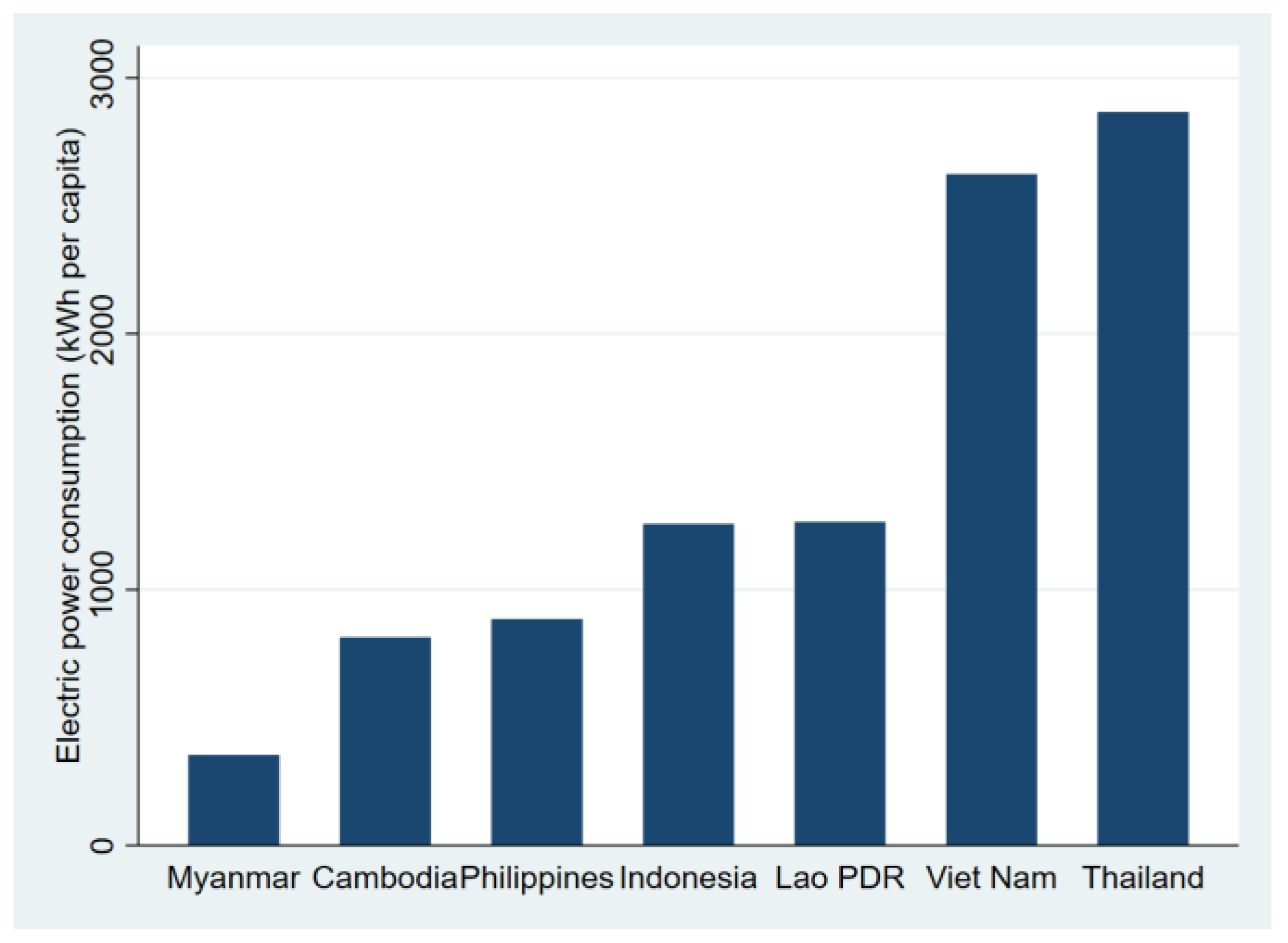
  1. World Bank. Electric Power Consumption (kWh Per Capita); World Bank Group: Washington, DC, USA, 2022; Available online: https://data.worldbank.org/indicator/EG.USE.ELEC.KH.PC?end=2023&name_desc=false&start=2023&year=2022 (accessed on 30 March 2025).
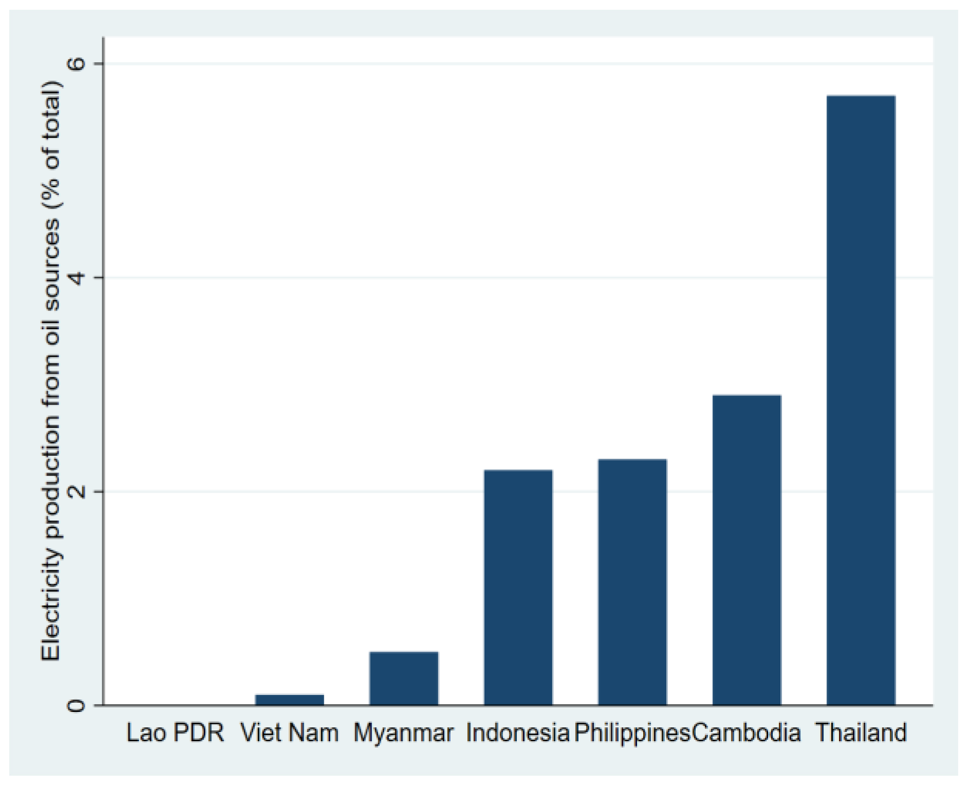
  2. World Bank. Electricity Production From Oil Sources (% of Total); World Bank Group: Washington, DC, USA, 2022; Available online: https://data.worldbank.org/indicator/EG.ELC.PETR.ZS?end=2023&name_desc=false&start=2023&year=2022 (accessed on 30 March 2025).
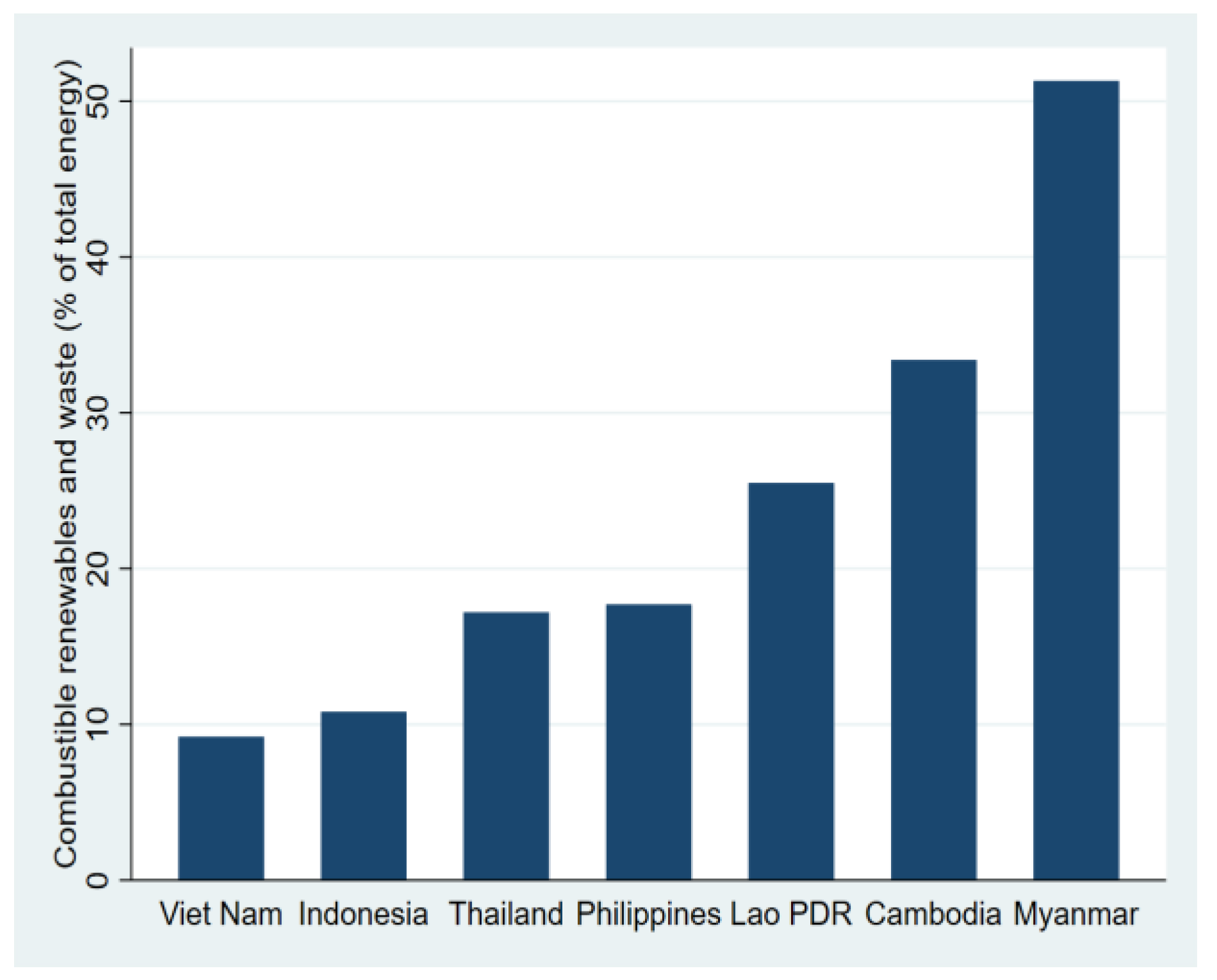
  3. World Bank. Combustible Renewables and Waste (% of Total Energy); World Bank Group: Washington, DC, USA, 2022; Available online: https://data.worldbank.org/indicator/EG.USE.CRNW.ZS?end=2023&name_desc=false&start=2023&year=2022 (accessed on 30 March 2025).
  4. Tunpaiboon, N. Business/Industry Trends 2025–2027: Electricity Generation Business; Krungsri Research: Bangkok, Thailand, 2024; Available online: https://www.krungsri.com/th/research/industry/industry-outlook/energy-utilities/power-generation/io/power-generation-2025-2027 (accessed on 29 March 2025).
  5. EPPO. Electricity Consumption by Sectors 2015–2022; Energy Policy and Planning Office: Bangkok, Thailand, 2022; Available online: https://www.eppo.go.th/index.php/en/en-energystatistics/electricity-statistic/Electricity%20Consumption%20for%20the%20Whole%20Country%20(Classified%20by%20Sector) (accessed on 30 March 2025).
  6. Phadkantha, R.; Yamaka, W. The nonlinear impact of electricity consumption on economic growth: Evidence from Thailand. Energy Rep. 2022, 8, 1315–1321. [Google Scholar] [CrossRef]
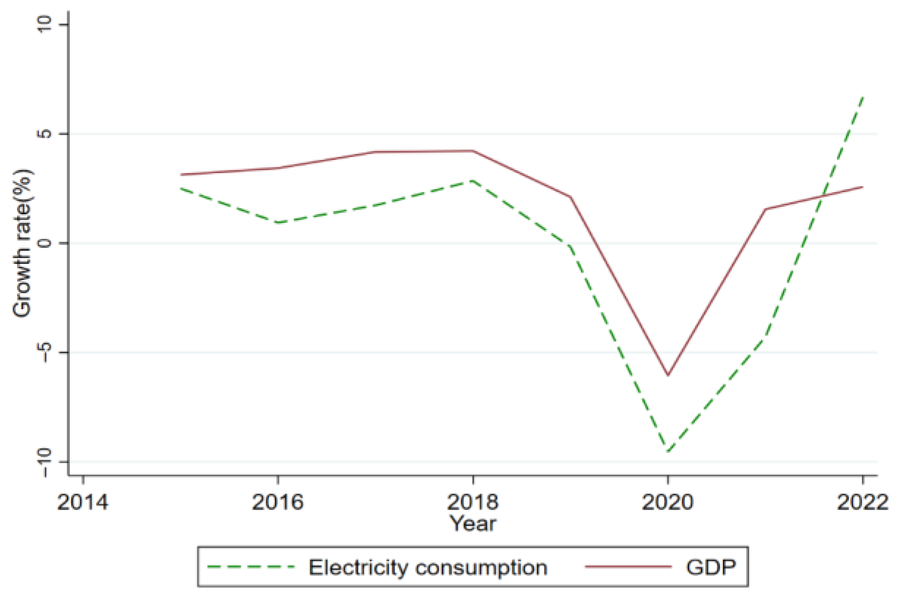
  7. EPPO. Growth Rate of Electricity Demand and Economic Growth 2015-2022; Energy Policy and Planning Office: Bangkok, Thailand, 2022; Available online: https://www.eppo.go.th/index.php/en/en-energystatistics/electricity-statistic/Power%20Generation%20Classified%20by%20Fuel%20Type%20(Detail)%20-%20Graph (accessed on 30 March 2025).
  8. EPPO. Power Generation (GWh) by Fuel 2015–2022; Energy Policy and Planning Office: Bangkok, Thailand, 2022; Available online: https://www.eppo.go.th/index.php/en/en-energystatistics/electricity-statistic/Power%20Generation%20Classified%20by%20Fuel%20Type (accessed on 30 March 2025).
  9. Chokchaichamnankit, S. Energy Projects Under the ASEAN Economic Community; Thai Climate Justice Organization: Chiang Mai, Thailand, 2012; Available online: https://www.thaiclimatejustice.org/sites/default/files/2012-08_โครงการด้านพลังงานภายใต้ประชาคมเศรษฐกิจอาเซียน.pdf (accessed on 3 January 2025).
  10. EGAT. Get to Know ASEAN Electricity; Electricity Generating Authority of Thailand: Nonthaburi, Thailand, 2016; Available online: https://www.thaigov.go.th/uploads/document/66/2017/02/pdf/Coal_power_plant_5.pdf (accessed on 30 March 2025).
  11. Fiscal Policy Office. Regional Fiscal Economic Report for November 2022; Fiscal Policy Office: Bangkok, Thailand, 2022; Available online: https://www.fpo.go.th/main/Economic-report/Monthly-regional-economic-situation/17261.aspx (accessed on 3 January 2025).
  12. NESDC. Gross Regional and Provincial Product (GPP); Office of the National Economic and Social Development Council: Bangkok, Thailand, 2022; Available online: https://www.nesdc.go.th/nesdb_en/more_news.php?cid=156&filename=index (accessed on 3 January 2025).
  13. EPPO. Electricity Consumption Per Capita; Energy Policy and Planning Office: Bangkok, Thailand, 2022; Available online: https://www.eppo.go.th/index.php/en/en-energystatistics/electricity-statistic/Electricity%20Consumption%20in%20PEA%20Area%20(Classified%20by%20Sector) (accessed on 30 March 2025).
  14. Arouri, M.; Shahbaz, M.; Onchang, R.; Islam, F.; Teulon, F. Environmental Kuznets curve in Thailand: Cointegration and causality analysis. J. Energy Dev. 2013, 39, 149–170. [Google Scholar]
  15. Azam, M.; Khan, A.Q.; Zaman, K.; Ahmad, M. Factors determining energy consumption: Evidence from Indonesia, Malaysia and Thailand. Renew. Sustain. Energy Rev. 2015, 42, 1123–1131. [Google Scholar] [CrossRef]
  16. Kyophilavong, P.; Shahbaz, M.; Anwar, S.; Masood, S. The energy-growth nexus in Thailand: Does trade openness boost up energy consumption? Renew. Sustain. Energy Rev. 2015, 46, 265–274. [Google Scholar] [CrossRef]
  17. Maneejuk, N.; Ratchakom, S.; Maneejuk, P.; Yamaka, W. Does the environmental Kuznets curve exist? An international study. Sustainability 2020, 12, 9117. [Google Scholar] [CrossRef]
  18. Phrakhruopatnontakitti, P.; Watthanabut, B.; Jermsittiparsert, K. Energy consumption, economic growth and environmental degradation in 4 Asian Countries: Malaysia, Myanmar, Vietnam and Thailand. Int. J. Energy Econ. Policy 2020, 10, 529–539. [Google Scholar] [CrossRef]
  19. Maneejuk, P.; Yamaka, W.; Sriboonchitta, S. Does the Kuznets curve exist in Thailand? A two decades’ perspective (1993–2015). Ann. Oper. Res. 2021, 300, 545–576. [Google Scholar] [CrossRef]
  20. Kuznets, S. International differences in capital formation and financing. In Capital Formation and Economic Growth; Princeton University Press: Princeton, NJ, USA, 1955; pp. 19–111. [Google Scholar]
  21. Grossman, G.M.; Krueger, A.B. Economic Growth and the Environment. Q. J. Econ. 1995, 110, 353–377. [Google Scholar] [CrossRef]
  22. Stern, D.I. The environmental Kuznets curve after 25 years. J. Bioeconom. 2017, 19, 7–28. [Google Scholar] [CrossRef]
  23. Panayotou, T. Demystifying the environmental Kuznets curve: Turning a black box into a policy tool. Environ. Dev. Econ. 1997, 2, 465–484. [Google Scholar] [CrossRef]
  24. Stern, D.I. The rise and fall of the environmental Kuznets curve. World Dev. 2004, 32, 1419–1439. [Google Scholar] [CrossRef]
  25. Suri, V.; Chapman, D. Economic growth, trade and energy: Implications for the environmental Kuznets curve. Ecol. Econ. 1998, 25, 195–208. [Google Scholar] [CrossRef]
  26. Lorente, D.; Alvarez-Herranz, A. An approach to the effect of energy innovation on environmental Kuznets curve: An introduction to inflection point. Bull. Energy Econ. 2016, 4, 224–233. [Google Scholar]
  27. Dasgupta, S.; Laplante, B.; Wang, H.; Wheeler, D. Confronting the environmental Kuznets curve. J. Econ. Perspect. 2002, 16, 147–168. [Google Scholar] [CrossRef]
  28. Ang, J.B. CO2 emissions, energy consumption, and output in France. Energy Policy 2007, 35, 4772–4778. [Google Scholar] [CrossRef]
  29. Halicioglu, F. An econometric study of CO2 emissions, energy consumption, income and foreign trade in Turkey. Energy Policy 2009, 37, 1156–1164. [Google Scholar] [CrossRef]
  30. Chandran, V.; Tang, C.F. The impacts of transport energy consumption, foreign direct investment and income on CO2 emissions in ASEAN-5 economies. Renew. Sustain. Energy Rev. 2013, 24, 445–453. [Google Scholar] [CrossRef]
  31. Al-Mulali, U.; Saboori, B.; Ozturk, I. Investigating the environmental Kuznets curve hypothesis in Vietnam. Energy Policy 2015, 76, 123–131. [Google Scholar] [CrossRef]
  32. Pablo-Romero, M.d.P.; De Jesús, J. Economic growth and energy consumption: The energy-environmental Kuznets curve for Latin America and the Caribbean. Renew. Sustain. Energy Rev. 2016, 60, 1343–1350. [Google Scholar] [CrossRef]
  33. Kurniawan, R.; Managi, S. Coal consumption, urbanization, and trade openness linkage in Indonesia. Energy Policy 2018, 121, 576–583. [Google Scholar] [CrossRef]
  34. Nguyen, K.H.; Kakinaka, M. Renewable energy consumption, carbon emissions, and development stages: Some evidence from panel cointegration analysis. Renew. Energy 2019, 132, 1049–1057. [Google Scholar] [CrossRef]
  35. Hien, P. Excessive electricity intensity of Vietnam: Evidence from a comparative study of Asia-Pacific countries. Energy Policy 2019, 130, 409–417. [Google Scholar] [CrossRef]
  36. Kibria, A.; Akhundjanov, S.B.; Oladi, R. Fossil fuel share in the energy mix and economic growth. Int. Rev. Econ. Financ. 2019, 59, 253–264. [Google Scholar] [CrossRef]
  37. Shahzad, Q.; Aruga, K. Spatial effect of economic performance on the ecological footprint: Evidence from Asian countries. Environ. Dev. Sustain. 2024. [Google Scholar] [CrossRef]
  38. Ozcan, B. The nexus between carbon emissions, energy consumption and economic growth in Middle East countries: A panel data analysis. Energy Policy 2013, 62, 1138–1147. [Google Scholar] [CrossRef]
  39. Wang, S.S.; Zhou, D.Q.; Zhou, P.; Wang, Q. CO2 emissions, energy consumption and economic growth in China: A panel data analysis. Energy Policy 2011, 39, 4870–4875. [Google Scholar] [CrossRef]
  40. Dyrstad, J.M.; Skonhoft, A.; Christensen, M.Q.; Ødegaard, E.T. Does economic growth eat up environmental improvements? Electricity production and fossil fuel emission in OECD countries 1980–2014. Energy Policy 2019, 125, 103–109. [Google Scholar] [CrossRef]
  41. Deichmann, U.; Reuter, A.; Vollmer, S.; Zhang, F. The relationship between energy intensity and economic growth: New evidence from a multi-country multi-sectorial dataset. World Dev. 2019, 124, 104664. [Google Scholar] [CrossRef]
  42. Borozan, D. Unveiling the heterogeneous effect of energy taxes and income on residential energy consumption. Energy Policy 2019, 129, 13–22. [Google Scholar] [CrossRef]
  43. Aruga, K. Investigating the energy-environmental Kuznets Curve hypothesis for the Asia-Pacific region. Sustainability 2019, 11, 2395. [Google Scholar] [CrossRef]
  44. Srisaringkarn, T.; Aruga, K. The Spatial Impact of PM2.5 Pollution on Economic Growth from 2012 to 2022: Evidence from Satellite and Provincial-Level Data in Thailand. Urban Sci. 2025, 9, 110. [Google Scholar] [CrossRef]
  45. Aslanidis, N.; Xepapadeas, A. Smooth ‘Inverted-V-Shaped’ & Smooth ‘N-Shaped’ Pollution-Income Paths; University of Crete: Rethymno, Greece, 2004. [Google Scholar]
  46. Sinha Babu, S.; Datta, S.K. The relevance of environmental Kuznets curve (EKC) in a framework of broad-based environmental degradation and modified measure of growth–a pooled data analysis. Int. J. Sustain. Dev. World Ecol. 2013, 20, 309–316. [Google Scholar] [CrossRef]
  47. Mahmood, H.; Alkhateeb, T.T.Y.; Tanveer, M.; Mahmoud, D.H. Testing the energy-environmental Kuznets curve hypothesis in the renewable and nonrenewable energy consumption models in Egypt. Int. J. Environ. Res. Public Health 2021, 18, 7334. [Google Scholar] [CrossRef] [PubMed]
  48. Zhang, B.; Wang, B.; Wang, Z. Role of renewable energy and non-renewable energy consumption on EKC: Evidence from Pakistan. J. Clean. Prod. 2017, 156, 855–864. [Google Scholar] [CrossRef]
  49. Marques, A.C.; Fuinhas, J.A.; Leal, P.A. The impact of economic growth on CO2 emissions in Australia: The environmental Kuznets curve and the decoupling index. Environ. Sci. Pollut. Res. 2018, 25, 27283–27296. [Google Scholar] [CrossRef]
  50. Mahmood, H. The effects of natural gas and oil consumption on CO2 emissions in GCC countries: Asymmetry analysis. Environ. Sci. Pollut. Res. 2022, 29, 57980–57996. [Google Scholar] [CrossRef]
  51. Anselin, L. Spatial Econometrics: Methods and Models; Springer Science & Business Media: Dordrecht, The Netherland, 1988. [Google Scholar]
  52. Wang, Y.; Li, K.; Xu, X.; Zhang, Y. Transport energy consumption and saving in China. Renew. Sustain. Energy Rev. 2014, 29, 641–655. [Google Scholar] [CrossRef]
  53. Neves, S.A.; Marques, A.C.; Fuinhas, J.A. Is energy consumption in the transport sector hampering both economic growth and the reduction of CO2 emissions? A disaggregated energy consumption analysis. Transp. Policy 2017, 59, 64–70. [Google Scholar] [CrossRef]
  54. Auffhammer, M.; Mansur, E.T. Measuring climatic impacts on energy consumption: A review of the empirical literature. Energy Econ. 2014, 46, 522–530. [Google Scholar] [CrossRef]
  55. Brown, C.; Meeks, R.; Ghile, Y.; Hunu, K. An Empirical Analysis of the Effects of Climate Variables on National Level Economic Growth; World Bank Policy Research Working Paper; World Bank: Washington DC, USA, 2010; Available online: https://ssrn.com/abstract=1645727 (accessed on 22 May 2025).
  56. Henseler, M.; Schumacher, I. The impact of weather on economic growth and its production factors. Clim. Change 2019, 154, 417–433. [Google Scholar] [CrossRef]
  57. Iamtrakul, P.; Chayphong, S. Factors affecting the development of a healthy city in Suburban areas, Thailand. J. Urban Manag. 2023, 12, 208–220. [Google Scholar] [CrossRef]
  58. Khanthavit, A. Instrumental-Variable Estimation of Bangkok-Weather Effects in the Stock Exchange of Thailand. Asian Acad. Manag. J. Account. Financ. 2017, 13, 83–111. [Google Scholar] [CrossRef]
  59. Nunta, J.; Sahachaisaeree, N. Cultural landscape, urban settlement and dweller’s perception: A case study of a vernacular village in Northern Thailand. Procedia-Soc. Behav. Sci. 2012, 42, 153–158. [Google Scholar] [CrossRef]
  60. Sarkodie, S.A.; Ahmed, M.Y.; Owusu, P.A. Ambient air pollution and meteorological factors escalate electricity consumption. Sci. Total Environ. 2021, 795, 148841. [Google Scholar] [CrossRef]
  61. Siriwashiraporn, A. Factors Affecting the Existence of Traditional Settlement of Pak Klong Wat Pradu Community, Samut Songkhram and Ratcha Buri Provinces; Chulalongkorn Univeristy: Bangkok, Thailand, 2007. [Google Scholar]
  62. Soytong, P.; Janchidfa, K.; Chayhard, S.; Phengphit, N. Analysis of Climate Change Impacts on Water Resource, Urban, and Human Settlements in Eastern Thailand: Geo-Informatics Approach for Climate Change Studies; Faculty of Geoinformatics, Burapha University: Chon Buri, Thailand, 2019; Available online: http://dspace.lib.buu.ac.th/xmlui/handle/1234567890/3888 (accessed on 22 May 2025).
  63. Wan, W.; Wang, J. The Impact of Weather on Economic Growth: County-Level Evidence from China. Sustainability 2024, 16, 9988. [Google Scholar] [CrossRef]
  64. Zhang, M.; Zhang, K.; Hu, W.; Zhu, B.; Wang, P.; Wei, Y.-M. Exploring the climatic impacts on residential electricity consumption in Jiangsu, China. Energy Policy 2020, 140, 111398. [Google Scholar] [CrossRef]
  65. Moran, P.A. The interpretation of statistical maps. J. R. Stat. Society. Ser. B (Methodol.) 1948, 10, 243–251. [Google Scholar] [CrossRef]
  66. Getis, A.; Ord, J.K. The analysis of spatial association by use of distance statistics. Geogr. Anal. 1992, 24, 189–206. [Google Scholar] [CrossRef]
  67. Baltagi, B.H. A Companion to Theoretical Econometrics(Chapter Fourteen Spatial Econometrics); Wiley Online Library: Hoboken, NJ, USA, 2001. [Google Scholar]
  68. Elhorst, J.P. Unconditional maximum likelihood estimation of linear and log-linear dynamic models for spatial panels. Geogr. Anal. 2005, 37, 85–106. [Google Scholar] [CrossRef]
  69. Yu, J.; De Jong, R.; Lee, L.-f. Quasi-maximum likelihood estimators for spatial dynamic panel data with fixed effects when both n and T are large. J. Econom. 2008, 146, 118–134. [Google Scholar] [CrossRef]
  70. Elhorst, J.P. Spatial Econometrics: From Cross-Sectional Data to Spatial Panels; Springer: Berlin/Heidelberg, Germany, 2014. [Google Scholar] [CrossRef]
  71. LeSage, J.; Pace, R.K. Introduction to Spatial Econometrics; Chapman and Hall/CRC: Boca Raton, FL, USA, 2009. [Google Scholar] [CrossRef]
  72. Bouayad-Agha, S.; Vedrine, L. Estimation strategies for a spatial dynamic panel using GMM. A new approach to the convergence issue of European regions. Spat. Econ. Anal. 2010, 5, 205–227. [Google Scholar] [CrossRef]
  73. Kripfganz, S.; Sarafidis, V. Estimating Spatial Dynamic Panel Data Models with Unobserved Common Factors in Stata. J. Stat. Softw. 2025. [Google Scholar] [CrossRef]
  74. Murshed, M. Are Trade Liberalization policies aligned with Renewable Energy Transition in low and middle income countries? An Instrumental Variable approach. Renew. Energy 2020, 151, 1110–1123. [Google Scholar] [CrossRef]
  75. Chen, X.; Chen, M. Energy, environment and industry: Instrumental approaches for environmental regulation on energy efficiency. Environ. Impact Assess. Rev. 2024, 105, 107439. [Google Scholar] [CrossRef]
  76. Siddiquee, M.; Ahamed, R. Exploring water consumption in Dhaka city using instrumental variables regression approaches. Env. Process 2020, 7, 1255–1275. [Google Scholar] [CrossRef]
  77. Karmaker, S.C.; Barai, M.K.; Sen, K.K.; Saha, B.B. Effects of remittances on renewable energy consumption: Evidence from instrumental variable estimation with panel data. Util. Policy 2023, 83, 101614. [Google Scholar] [CrossRef]
  78. Li, L.; Sun, W.; Hu, W.; Sun, Y. Impact of natural and social environmental factors on building energy consumption: Based on bibliometrics. J. Build. Eng. 2021, 37, 102136. [Google Scholar] [CrossRef]
  79. Hastie, T.; Tibshirani, R. Generalized additive models. Stat. Sci. 1986, 1, 297–310. [Google Scholar] [CrossRef]
  80. Bank of Thailand. Thai Economic Condition Report for 2022; Bank of Thailand: Bangkok, Thailand, 2022; Available online: https://www.bot.or.th/content/dam/bot/documents/th/thai-economy/state-of-thai-economy/annual-report/annual-econ-report-th-2565.pdf (accessed on 10 January 2025).
  81. NESDC. Thai Economic Performance in Q4 and 2022 and Outlook for 2023 (English Edition); Office of the National Economic and Social Development Council: Bangkok, Thailand, 2022; Available online: https://www.nesdc.go.th/nesdb_en/article_attach/65Q4%20Press%20Eng%20Q4-2022%20(2102%2015.46).pdf (accessed on 10 January 2025).
  82. Trakulchavalit, C. A Comparative Study on Housing and Behavior of Graduated From USA UK and Japan; Chulalongkorn University: Bangkok, Thailand, 1998. [Google Scholar]
  83. Chevaporanapiwat, C. Factors Affecting Changes in Human Settlements in Bang Lum-Poo District; Chulalongkorn University: Bangkok, Thailand, 2001. [Google Scholar]
  84. Algarni, S.; Tirth, V.; Alqahtani, T.; Alshehery, S.; Kshirsagar, P. Contribution of renewable energy sources to the environmental impacts and economic benefits for sustainable development. Sustain. Energy Technol. Assess. 2023, 56, 103098. [Google Scholar] [CrossRef]
  85. Aruga, K.; Islam, M.M.; Jannat, A. Assessing the CO2 emissions and energy source consumption nexus in Japan. Sustainability 2024, 16, 5742. [Google Scholar] [CrossRef]
  86. Dincer, I. Renewable energy and sustainable development: A crucial review. Renew. Sustain. Energy Rev. 2000, 4, 157–175. [Google Scholar] [CrossRef]
  87. Mohtasham, J. Renewable energies. Energy Procedia 2015, 74, 1289–1297. [Google Scholar] [CrossRef]
Figure 1. Electric power consumption (kWh per capita) in 2022. Source: World Bank [1].
Energies 18 03980 g001
Figure 2. Electricity production from oil sources (% of total) in 2022. Source: World Bank [2].
Energies 18 03980 g002
Figure 3. Combustible renewables and waste (% of total energy) in 2022. Source: World Bank [3].
Energies 18 03980 g003
Figure 4. Electricity consumption by sector for 2015–2022. Source: Energy Policy and Planning Office (EPPO [5]).
Energies 18 03980 g004
Figure 5. Growth rate of electricity demand and economic growth for 2015–2022. Source: Energy Policy and Planning Office (EPPO [7]).
Energies 18 03980 g005
Figure 6. (a) Power generation (GWh) by fuel in 2015; (b) power generation (GWh) by fuel in 2022. Source: Energy Policy and Planning Office (EPPO [8]).
Energies 18 03980 g006
Figure 7. Thailand map. Source: Authors.
Energies 18 03980 g007
Figure 8. Overview of the steps of the methods. Source: Authors.
Energies 18 03980 g008
Figure 9. Hot spot analysis. Source: Authors.
Energies 18 03980 g009
Figure 10. GAM analysis: Three-dimensional effect graph of the driving factors of the variation in energy consumption per capita; (a) GPPpc and Landtemp_night; (b) GPPpc and Rainfall; (c) GPPpc and Windspeed; (d) GPPpc and Roaddens; (e) Landtemp_night and Windspeed; (f) Landtemp_night and Roaddens. Source: Authors.
Energies 18 03980 g010
Table 1. Gross regional product (GRP), GRP per capita, energy consumption, and energy consumption per capita by region (USD).
Regions2022 GRP2022 GRP per Capita2022 Average Energy Consumption (GWh)2022 Average Energy Consumption
(per Capita)
(kWh/person)
Northeastern (NE)USD 498 billionUSD 27241,162,050,0001101
Northern (NO)USD 373 billionUSD 3329990,185,0721436
Southern (SO)USD 394 billionUSD 40531,207,050,0001688
Bangkok and Vicinity (BKK&VIC)USD 2.2 trillionUSD 13,2107,554,832,7043861
Integrated Regions
BKK&VIC, CE, EA, WEUSD 3.6 trillionUSD 40,8575,212,023,9133970
Source: Office of the National Economic and Social Development Council (NESDC [12]), Energy Policy and Planning Office (EPPO [13]).
Table 2. A review of the relationship between economic growth and energy consumption.
EKC PatternsAuthorsDependent VariablesIndependent Variables
Monotonically rising curveDasgupta, et al. [27], Ang [28], Halicioglu [29], Chandran and Tang [30], Al-Mulali, et al. [31], Pablo-Romero and De Jesús [32]Energy use, annual emissions of CO2Gross value added per capita (GVApc), share of agriculture employment, foreign direct investment (FDI), transport energy consumption, labor force, exports and imports
Inverted U-shapeSuri and Chapman [25], Kurniawan and Managi [33], Nguyen and Kakinaka [34], Hien [35], Kibria, et al. [36], Maneejuk, et al. [17], Shahzad and Aruga [37]Energy per capita, coal consumption, renewable energy consumption, non-renewable energy consumption, electricity consumption, CO2 emissionReal GDP, manufacturing value added (MVA), industrial value added (IVA), import, export, urbanization, share of secondary industry value added, trade openness, real oil price in country, fossil fuel share, population density
U-shapeOzcan [38], Chandran and Tang [30], Wang, et al. [39], Dyrstad, et al. [40], Deichmann, et al. [41], Borozan [42], Aruga [43], Srisaringkarn and Aruga [44]Electricity production, energy intensity, energy consumption in households per capita, annual emissions of CO2, SO2, suspended particulate matterGDP, non-fossil energy, fossil energy, percentage of total energy consumption used in industry, transport, residential, services, agriculture and nonenergy use, energy taxes, energy prices, tertiary education, risk of poverty, climate conditions, population density
N-shapeGrossman and Krueger [21], Aslanidis and Xepapadeas [45], Sinha Babu and Datta [46], Mahmood, et al. [47]Primary energy, oil, natural gas, coal consumption, hydroelectricity consumption, air quality indexGRP per capita, GRP, GRP square, GRP cubic, temperature, import shares, share of the tertiary industry, environmental degradation index and population
Table 3. Data description.
TypesVariablesDescriptionsYearsSourcesExpected SignReferences
Dependent Variable E n e r g y   c o n s u m p t i o n  
p e r   c a p i t a  
( E n e r g y c o n s _ p c )
A variable that represents a province’s economic activity using electricity consumption per capita as an indicator (kWh/person)2015–2022Metropolitan Electricity Authority (MEA),
Provincial Electricity Authority (PEA), and Electricity Generating Authority of Thailand (EGAT)
Independent Variables G r o s s   P r o v i n c i a l   P r o d u c t
p e r   c a p i t a   ( G P P p c )
A variable that represents economic growth per capita in each province; reflects the level of economic output per person in that province (baht/person)2015–2022Office of the National Economic and Social Development Council (NESDC)+/−[30,38,43,44]
P o p u l a t i o n   d e n s i t y  
( P o p _ d e n s )
A variable that represents a province’s population density; indicates how many people live per unit of area in that province (unit/km2)2015–2022Office of the National Economic and Social Development Council (NESDC)+[33,36,41]
R o a d   d e n s i t y   ( R o a d d e n s ) A variable that represents the road density of a province in a given year (length)2015–2022Geofabrik+[30,52,53]
Instrumental Variables L a n d   s u r f a c e   t e m p e r a t u r e
a t   N i g h t  
( L a n d t e m p _ n i g h t )
A variable that represents a province’s land surface temperature at night; indicates how high the surface temperature is during nighttime in that province (Celcius)2015–2022MOD11A1.061 Terra Land Surface Temperature and Emissivity Daily Global 1km; bands: LST_Night_1km [54,55,56,57,58,59,60,61,62,63,64]
R a i n f a l l
( R a i n f a l l )
A variable that shows the average annual rainfall in a province (mm/y) (millimeters/year)2015–2022CHIRPS Daily: Climate Hazards Center InfraRed Precipitation With Station Data (Version 2.0 Final); bands: precipitation [54,55,56,57,58,59,60,61,62,63,64]
W i n d s p e e d
( W i n d s p e e d )
A variable that shows the average annual wind speed and direction in a province (m/s) (meters per second)2015–2022GLDAS-2.1: Global Land Data Assimilation System; bands: Wind_f_inst [54,55,56,58,60,63,64]
Table 4. Moran’s I statistical test for the year 2022.
Variable:
Energy Consumption per Capita
(Energycons_pc)
Whole RegionBKK&VIC, CE, EA, WENENOSO
Moran’s I0.6580.9320.9610.8840.994
E(I)−0.013−0.013−0.013−0.013−0.013
SE(I)0.0880.0910.0940.0940.089
Z(I)7.69010.41910.3639.50711.269
p-value0.0010.0010.0010.0010.001
Table 5. Spatial correlation test results.
TestsStatisticdfp-Value
Moran’s I2.55410.011
Spatial Error
Lagrange multiplier1.40610.236
Robust Lagrange multiplier1.21210.271
Spatial Lag
Lagrange multiplier2.15410.142
Robust Lagrange multiplier1.96110.161
Table 6. Regression results of the Spatial Panel Lag and Spatial Dynamic Panel Lag IV Fixed-Effects Models.
Variables:
LnEnergycons_pc
Static Spatial Panel Lag Model
(Whole Region)
Spatial Dynamic Panel Lag IV Model
(Whole Region)
Model 1Model 2Model 3Model 4
LnEnergycons_pc(−1)na −0.074
(−1.13)
−0.087
(−1.36)
−0.081
(−1.36)
LnGPPpc2.060
(4.75)
***0.372
(5.53)
*** −1.979
(−2.04)
**
LnGPPpc2−0.070
(−3.92)
*** 0.016
(6.07)
***0.096
(2.44)
**
LnPop_dens−0.753
(−8.42)
***13.117
(1.62)
9.108
(1.69)
*6.336
(2.06)
**
LnLandtemp_night−2.572
(−2.10)
**na na na
LnRainfall0.013
(1.01)
na na na
LnWindspeed0.012
(0.46)
na na na
LnRoaddens0.023
(3.86)
***0.023
(1.50)
0.023
(1.52)
0.017
(1.09)
COVID−0.001
(−0.06)
0.011
(1.75)
*0.011
(1.78)
*0.006
(0.84)
Spatial rho ( ρ ) 0.336
(7.39)
***0.372
(2.48)
**0.347
(2.34)
**0.327
(2.02)
**
Obs616462462462
Instruments nb. 181818
Hansen J 14.14713.76810.450
(Hansen J p-value) (0.291)(0.316)(0.490)
AIC−1840.591
BIC−1796.359
RMSE20.88912.7038.8576.225
MAE20.8629.3026.6784.860
Note: z-statistics are reported in parentheses. * p < 0.10, ** p < 0.05, *** p < 0.01.
Table 7. Regression results of the Spatial Dynamic Panel Lag IV Fixed-Effects Model (regions).
Variables:
LnEnergycons_pc
BKK&VIC, CE, EA, WEVariablesNE
Coef.Z-StatCoef.Z-Stat
Intercept48.986***3.33Intercept58.134***2.79
LnEnergycons_pc(−1)0.495***4.43LnEnergycons_pc(−1)0.151***3.38
LnGPPpc−7.788***−5.53LnGPPpc−10.977***−2.79
LnGPPpc20.319***5.63LnGPPpc20.481***2.76
LnPop_dens−0.353 −0.91LnPop_dens1.144 0.86
LnRoaddens0.022*1.72LnRoaddens0.010***3.44
Spatial rho ( ρ ) 0.631***2.61Spatial rho ( ρ ) 0.787***7.21
Obs 156 Obs 120
Instruments nb. 18 Instruments nb. 18
Hansen J 10.063 Hansen J 10.634
(Hansen J p-value) 0.611 (Hansen J p-value) 0.561
VariablesNOVariablesSO
Coef.Z-statCoef.Z-stat
Intercept−29.319 −0.67Intercept−3.996 −0.65
LnEnergycons_pc(−1)0.297***3.77LnEnergycons_pc(−1)0.051 0.37
LnGPPpc4.889 1.23LnGPPpc0.531 0.34
LnGPPpc2−0.211 −1.24LnGPPpc2−0.011 −0.17
LnPop_dens0.251 1.11LnPop_dens0.653 0.71
LnRoaddens0.025**2.06LnRoaddens0.034***3.92
Spatial rho ( ρ ) 0.731***5.87Spatial rho ( ρ ) 0.411***4.46
Obs 102 Obs 84
Instruments nb. 17 Instruments nb. 14
Hansen J 8.201 Hansen J 7.327
(Hansen J p-value) 0.695 (Hansen J p-value) 0.502
Note: * p < 0.10, ** p < 0.05, *** p < 0.01.
Table 8. Effect analysis of the Spatial Dynamic Panel Lag IV Fixed-Effects Model.
Whole Region (n = 462)
VariablesShort-Run EffectZ-StatLong-Run EffectZ-Stat
DirectLnGPPpc−2.012**−2.04−1.856**−1.98
LnGPPpc20.097**2.440.090**2.35
LnPop_dens6.444**2.085.943**2.10
LnRoaddens0.017 1.090.016 1.11
COVID0.006 0.840.005 0.84
IndirectLnGPPpc−0.701 −1.15−0.582 −1.11
LnGPPpc20.034 1.230.028 1.19
LnPop_dens2.246 1.371.864 1.35
LnRoaddens0.006 0.890.005 0.87
COVID0.002 0.660.002 0.67
TotalLnGPPpc−2.713*−1.87−2.438*−1.82
LnGPPpc20.131**2.190.118**2.11
LnPop_dens8.690**2.127.801**2.13
LnRoaddens0.023 1.060.021 1.09
COVID0.008 0.800.007 0.81
Note: * p < 0.10, ** p < 0.05.
Table 9. The GAM hypothesis test for energy consumption per capita and the explanatory variables.
Estimated Degrees of FreedomF-Statisticp-Value
GPPpc-Landtemp_night56.439.6<0.01
GPPpc-Rainfall65.535.3<0.01
GPPpc-Windspeed76.010.6<0.01
GPPpc-Roaddens71.5247.5<0.01
Landtemp_night-Windspeed11.74.9<0.01
Landtemp_night-Roaddens5.18.8<0.01
Disclaimer/Publisher’s Note: The statements, opinions and data contained in all publications are solely those of the individual author(s) and contributor(s) and not of MDPI and/or the editor(s). MDPI and/or the editor(s) disclaim responsibility for any injury to people or property resulting from any ideas, methods, instructions or products referred to in the content.

