An Ensemble Model of Attention-Enhanced N-BEATS and XGBoost for District Heating Load Forecasting

Abstract

Accurate heat load forecasting is essential for the efficiency of District Heating Systems (DHS). Still, it is challenged by the need to model long-term temporal dependencies and nonlinear relationships with weather and other factors. This study proposes a hybrid deep learning framework combining an attention-enhanced Neural Basis Expansion Analysis for Time Series (N-BEATS) model and eXtreme Gradient Boosting (XGBoost). The N-BEATS component, with a multi-head self-attention mechanism, captures temporal dynamics, while XGBoost models non-linear impacts of external variables. Predictions are integrated using an optimized weighted averaging strategy. Evaluated on a dataset from 103 heating units, the model outperformed 13 baselines, achieving an MSE of 0.4131, MAE of 0.3732, RMSE of 0.6427, and R² of 0.9664. This corresponds to a reduction of 32.6% in MSE, 32.0% in MAE, and 17.9% in RMSE, and an improvement of 5.1% in R² over the best baseline. Ablation studies and statistical tests confirmed the effectiveness of the attention mechanism and ensemble strategy. This model provides an efficient solution for DHS load forecasting, facilitating optimized energy dispatch and enhancing system performance.

1. Introduction

District Heating Systems (DHSs) constitute a crucial element of modern urban infrastructure, significantly enhancing energy efficiency and advancing global carbon neutrality objectives [1,2]. As the core component of smart thermal grids, the operational optimization of DHSs critically depends on precise and reliable heat load forecasting. Accurate predictions facilitate proactive control and demand-side management, thereby reducing energy consumption and operational costs and ensuring the stability and resilience of the entire heating distribution network [3]. Consequently, developing high-performance heat load forecasting models has become an essential and widely studied research area.

However, heat load forecasting in DHSs remains a highly challenging task due to the inherent complexity and dynamism of the system. Various interacting factors influence heat load [4], including meteorological conditions (e.g., ambient temperature, solar radiation), building characteristics, and stochastic user behaviors, collectively leading to strong nonlinear and time-varying characteristics. Additionally, significant thermal inertia in heating networks introduces complex long-range temporal dependencies, complicating accurate modeling. Complex parameterizations and idealized assumptions often constrain traditional physical models. At the same time, earlier data-driven methods such as linear regression and AutoRegressive Integrated Moving Average (ARIMA) struggle to capture intricate nonlinear relationships and long-term dependencies, resulting in limited prediction accuracy and applicability in practical scenarios. Although various machine learning and deep learning models have been proposed, developing a single model capable of effectively addressing complex temporal dynamics and nonlinear relationships with exogenous variables simultaneously remains an ongoing challenge.

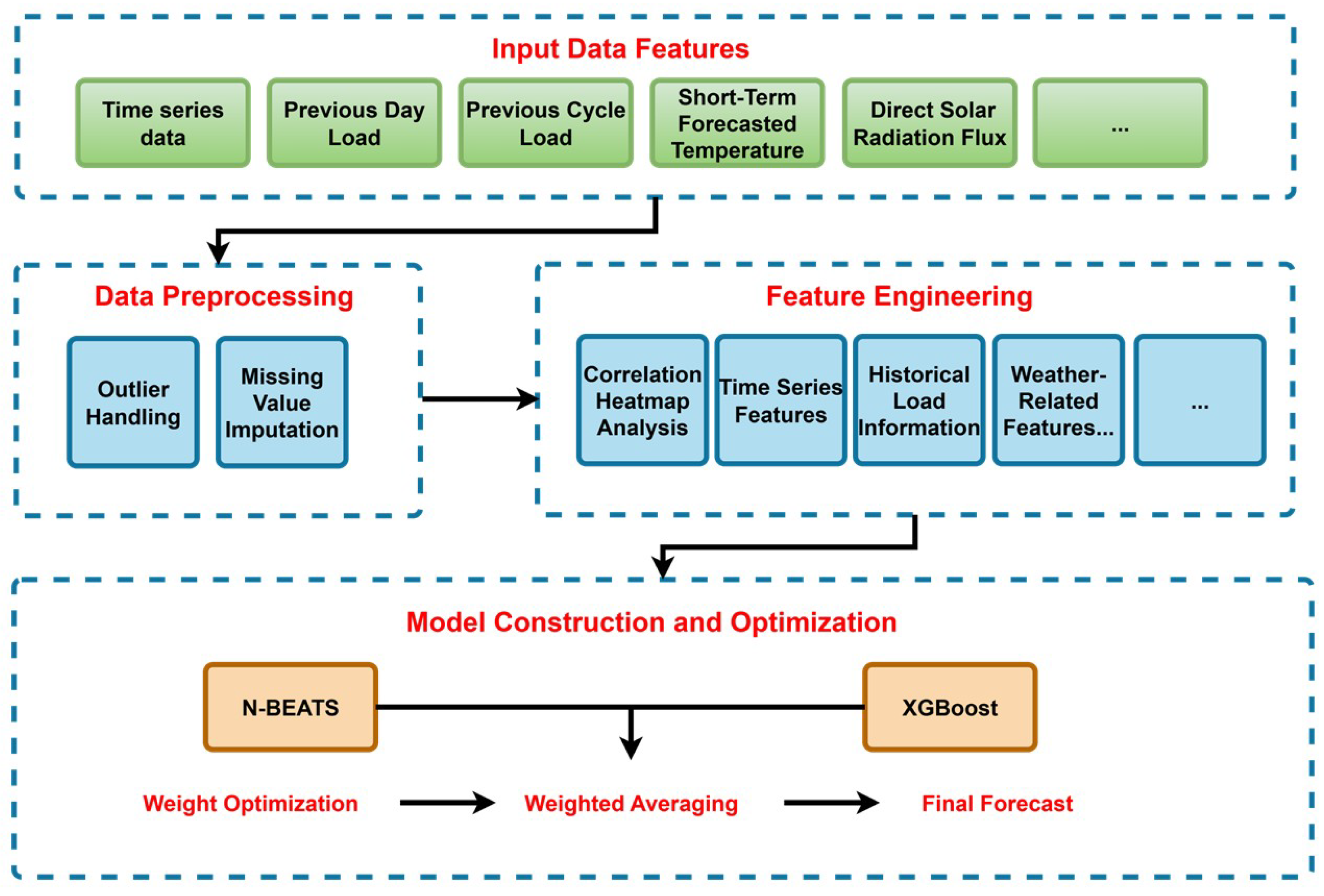
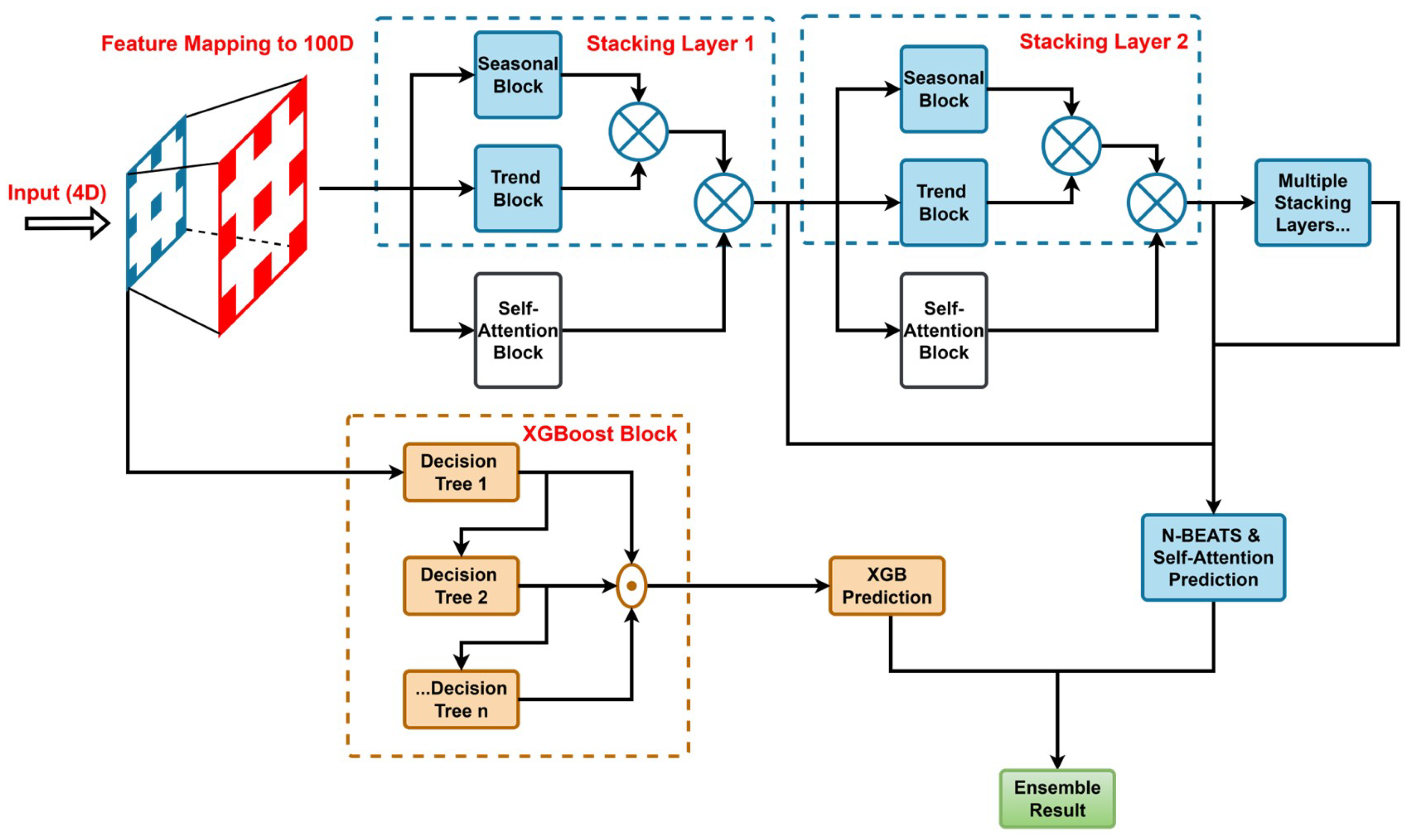
This paper proposes a novel hybrid forecasting model that synergistically integrates a deep learning architecture with the powerful gradient boosting machine to close this gap. Our approach aims explicitly to deconstruct and model the multifaceted characteristics of heat load data. The core of the model comprises two specialized components: (1) an N-BEATS (Neural Basis Expansion Analysis for Time Series) network enhanced by a multi-head self-attention mechanism designed to capture and interpret inherent trends, seasonality, and long-range dependencies within time series data, and (2) an XGBoost (Extreme Gradient Boosting) model, utilized for effectively learning complex nonlinear mappings between exogenous variables and heat load. These two components are seamlessly integrated through an optimized weighted ensemble strategy, enabling the final model to leverage the unique strengths of each part, thus achieving outstanding predictive accuracy.

The contributions of this research can be summarized in three points:

• A Novel Hybrid Framework with Complementary Strengths: We introduce a novel hybrid framework that synergistically combines two powerful models with distinct, complementary strengths. This architecture moves beyond simple model combination by leveraging (1) an attention-enhanced N-BEATS model, which excels at capturing intrinsic temporal dynamics such as trends, seasonality, and long-range dependencies arising from thermal inertia; (2) an XGBoost model, which is highly effective at modeling the complex, nonlinear impacts of exogenous variables (e.g., meteorological data). By integrating their predictions through an optimized weighting strategy, the framework capitalizes on the unique capabilities of each model to achieve superior forecasting accuracy.
• Methodological Innovation via Attention-Enhanced Temporal Modeling: We innovatively integrate a multi-head self-attention mechanism directly into the N-BEATS architecture. This enhancement is a targeted improvement for District Heating Systems, empowering the model to dynamically identify and weigh the significance of different historical time steps. This is critical for accurately modeling the long-range dependencies characteristic of systems with high thermal inertia, a capability validated by our ablation studies.
• Validation on Real-World Enterprise Data: We evaluated the proposed model using real heating operation data from 103 heat exchange stations. The experimental results demonstrate that the model outperforms 13 mainstream baseline models, achieving a Mean Squared Error (MSE) of 0.4131, Mean Absolute Error (MAE) of 0.3732, Root Mean Squared Error (RMSE) of 0.6427, and a Coefficient of Determination (R²) of 0.9664. This corresponds to a reduction of 32.6% in MSE, 32.0% in MAE, and 17.9% in RMSE, and an improvement of 5.1% in R² over the best baseline, demonstrating significant improvements in practical applications.

The remainder of this paper is organized as follows. Section 2 presents the literature review. Section 3 describes the methodology. Section 4 details the experiments results and analysis. Finally, Section 5 concludes the paper and discusses future research directions.

Table 1. List of acronyms and their full forms.

Acronym	Full Form
ARIMA	AutoRegressive Integrated Moving Average
CLSPM	Causal Long-Sequence Prediction Model
CNNs	Convolutional Neural Networks
DHS	District Heating System
D-Linear	Decomposition–Linear Model
DLinear-NPTS	D-Linear enhanced with Non-Parametric Time Series
DSWRF	Direct Short-Wave Radiation Flux
FEDformer	Frequency Enhanced Decomposed Transformer
GAT	Graph Attention Network
LSTM	Long Short-Term Memory
MAE	Mean Absolute Error
MGMI	Multi-Modal Graph and Multi-Scale Informer
MSE	Mean Squared Error
N-BEATS	Neural Basis Expansion Analysis for Time Series
PIH	Primary Instantaneous Heat
PSO	Particle Swarm Optimization
PRT	Primary Return Temperature
R2	Coefficient of Determination
RMSE	Root Mean Squared Error
RNN	Recurrent Neural Network
RoC	Rate of Change
SARIMA	Seasonal AutoRegressive Integrated Moving Average
SRT	Secondary Return Temperature
SST	Secondary Supply Temperature
STL	Seasonal and Trend decomposition using Loess
SVR	Support Vector Regression
XGBoost	eXtreme Gradient Boosting

is a list of abbreviations used in this manuscript.

2. Literature Review

Accurate prediction of regional heat load is critical for efficient, stable, and economical operation of heating systems. To address this challenge, diverse forecasting strategies have been proposed by academia and industry, including physical models based on thermodynamics and heat transfer principles [5], rapidly advancing data-driven methods, and methods combining physical principles with data-driven approaches [6]. This paper focuses on data-driven methods, aiming to explore their application in regional heat load forecasting. Accordingly, this literature review systematically synthesizes key developments in data analysis techniques and forecasting models within the data-driven framework.

2.1. Advances in Data Analysis Methods

High-quality data constitutes the cornerstone of precise forecasting; thus, systematic data preprocessing represents an indispensable preliminary step in heat load modeling. A comprehensive data preprocessing pipeline generally follows standardized procedures, including data cleaning (handling missing and anomalous values), data transformation (standardization and normalization), feature engineering (feature extraction and selection), and data partitioning.

In data cleaning, researchers have employed diverse strategies ranging from simple to sophisticated. For missing data, traditional methods such as interpolation remain in use; however, advanced approaches utilizing machine learning models for predictive imputation are increasingly adopted to improve filling accuracy. Regarding noise and outliers, conventional statistical methods such as the 3$\sigma$ criterion or weighted filtering are partially effective [7] but limited when handling complex asymmetrical data distributions. Consequently, anomaly detection methods based on prediction residuals have emerged as a promising research direction. For instance, Li et al. proposed using a CNN-GRU model for time series prediction and identifying significant deviations between predicted and actual values as anomalies, demonstrating enhanced sensitivity and accuracy in dynamic systems [8].

In feature engineering and selection, the goal is to extract the most informative predictors for forecasting targets while removing redundant or irrelevant variables. The Pearson correlation coefficient is commonly employed for analyzing linear relationships between features and target variables [9]. Additionally, time series decomposition techniques, such as Seasonal and Trend decomposition using Loess (STL), are widely applied to extract trends, seasonal patterns, and residual components from heat load data, aiding models to learn data patterns across multiple temporal scales better.

Finally, data transformation is essential for stable model training. Due to enormous differences in scales among features (e.g., temperature, flow rate, pressure), standardization or normalization methods are necessary to eliminate dimensional effects, accelerate convergence, and enhance model performance. These systematic preprocessing methods collectively constitute crucial theoretical and practical foundations for our data handling framework.

2.2. Development of Forecasting Models

Forecasting models have shifted from statistical to machine learning, particularly notable in heat load forecasting [10]. Below we elaborate on this model development trajectory.

2.2.1. Traditional Time Series Models

The ARIMA model is a classic time series forecasting method that combines autoregression, differencing, and moving average [11]. ARIMA is suitable for stationary time series data or data that can be made stationary through differencing, effectively capturing linear dependencies in time series. SARIMA (Seasonal ARIMA) is an extension of ARIMA, designed explicitly for handling seasonal time series data [12].

However, due to the complexity of heating systems, traditional time series models, such as ARIMA and SARIMA, are insufficient for addressing nonlinear factors such as changing weather conditions, user habits, and pipeline heat loss. Consequently, the accuracy and stability of traditional time series models are often limited in practical applications.

2.2.2. Machine Learning Models

In heat load forecasting, studies typically start with basic models such as Multiple Linear Regression (MLR) [13]. Nevertheless, MLR presumes a linear relationship between the dependent variable and each feature. Consequently, it often struggles with the complex nonlinear dynamics commonly observed in district heating systems.

To overcome this linear limitation, ensemble methods based on tree learners—such as Random Forests [14,15] and XGBoost—are receiving growing attention. Rather than depending on a single predictive equation, these models capture nonlinear interactions through the cooperation of multiple decision trees.

XGBoost is an efficient implementation of Gradient Boosting Decision Trees [16]. It builds new trees sequentially, approximating the optimal search direction at each step by performing a second-order Taylor expansion of the objective function involving both first-order gradients and second-order Hessians. L1/L2 regularization and pruning are explicitly embedded in the objective of curbing overfitting. Thanks to these optimizations, XGBoost excels at modeling complex nonlinear relationships and handling high-dimensional (especially non-sparse) data [17].

In summary, MLR provides an interpretable and straightforward baseline for heat load forecasting. By comparison, Random Forests and XGBoost, based on decision tree algorithms, utilize ensemble learning to capture nonlinear relationships among features better. This approach helps overcome the limitations of linear models and allows efficient processing of large, multivariate datasets.

2.2.3. Deep Learning Methods

Deep learning has revolutionized time series forecasting by automatically learning complex patterns and nonlinear relationships from large datasets. Among these methods, Long Short-Term Memory (LSTM) networks are a cornerstone, using gating mechanisms to capture long-term dependencies and mitigate gradient vanishing issues [18,19]. Variants like CLSPM further enhance LSTM performance by incorporating self-attention, improving modeling of very long sequences [20].

Convolutional Neural Networks (CNNs), originally for image recognition, have been adapted to time series forecasting, efficiently extracting local features and trends through sliding convolutional kernels [21,22].

Another strategy is time series decomposition. The N-BEATS model uses stacked residual blocks to iteratively forecast components without relying on predefined statistical structures, achieving high accuracy [23,24]. Similarly, the D-Linear model and its variants like DLinear-NPTS challenge the necessity of complex architectures by decomposing series into trend and residual components. They model these components with simple linear layers, proving highly effective and computationally efficient on many forecasting tasks [25].

In summary, by leveraging LSTM for long-term dependencies, CNN for local pattern extraction, and decomposition approaches like N-BEATS and D-Linear, deep learning methods capture complex nonlinear features and significantly improve forecast accuracy using historical heating and weather data.

2.2.4. Hybrid Models as a Research Hotspot

Hybrid models combine the strengths of multiple forecasting methods through ensemble learning or model fusion, improving accuracy and robustness. They effectively address complex nonlinearities and uncertainties in heating systems, making them a research hotspot in heat load forecasting.

A common approach is integrating machine learning models with metaheuristic optimization. The PSO-SVR model, for example, uses Particle Swarm Optimization (PSO) [26] to optimize Support Vector Regression (SVR) hyperparameters, capturing nonlinear relationships more effectively and achieving an average absolute error of just 4.6% in one study [27].

Recent trends focus on hybridizing deep learning architectures to jointly model spatial and temporal dependencies. The GAT–Informer model combines a Graph Attention Network (GAT) for learning inter-variable relationships with the Informer for long-sequence forecasting, demonstrating strong potential for heat load prediction [28]. Subsequent advancements in this area, such as FEDformer, further improve upon the Transformer architecture by employing attention mechanisms in the frequency domain to achieve linear complexity, making them highly efficient for very long-sequence forecasting [29].

The MGMI model explicitly captures spatial correlations among buildings via a Multi-Modal Graph (MG) and models temporal profiles using a Multi-Scale Informer (MI). By integrating both spatial and temporal information, MGMI significantly reduces prediction errors compared to single models and other hybrids, highlighting the power of advanced hybrid deep learning approaches [30].

Overall, hybrid models outperform single-model approaches in metrics such as MSE, RMSE, MAE, and R², offering better stability and generalization across different heating scenarios.

2.3. Research Gaps

A systematic review of the literature highlights a significant methodological gap in heat load forecasting, driven by the conflicting inductive biases of leading model families. Current research struggles to jointly model intrinsic temporal structures and complex nonlinearities within a unified framework.

This conflict manifests in the core assumptions of the two dominant modeling paradigms. Sequential models (e.g., LSTM, N-BEATS) excel at capturing temporal dependencies but are less effective at handling high-dimensional, non-sequential exogenous features, often leading to suboptimal utilization. Conversely, Tabular Learning Models (e.g., XGBoost) are powerful at modeling complex nonlinear interactions but lack mechanisms to capture the sequential nature of data, treating observations as independent and identically distributed (i.i.d.).

Existing hybrid models often rely on simplistic fusion methods (e.g., feature concatenation or prediction averaging), failing to address the fundamental differences between temporal signals and exogenous influences. Such premature blending can introduce noise and hamper learning efficiency.

Consequently, this paper aims to fill this gap by proposing a novel hybrid model that leverages the complementary strengths of both sequential and tabular learning paradigms. Instead of relying on a single model, we construct two specialized models in parallel: (1) an attention-enhanced N-BEATS model, designed to capture the full extent of temporal dynamics from historical load data, and (2) an XGBoost model, tailored to learn the complex, nonlinear relationships between the rich set of exogenous variables and the heat load. The predictions from these two models are then integrated using an optimized weighted averaging scheme. This architecture allows each model to focus on the data structures it handles best—temporal sequences for N-BEATS and feature interactions for XGBoost—creating a synergistic framework that moves beyond the current methodological impasse.

3. Methodology

To accurately predict the thermal load of regional heating systems, this study proposes a hybrid forecasting methodology based on a logical progression, with the overall framework shown in Figure 1. This methodology decomposes the complex forecasting task into two interconnected core stages:

First, data preprocessing and feature engineering (Section 3.1) serve as the cornerstone of the entire process. This stage aims to transform raw data into a clean, structured, and information-rich feature set. This step is a necessary prerequisite for subsequent modeling and directly determines the upper limit of the model’s performance.

Second, building upon the high-quality data, we proceed to the model construction and optimization (Section 3.2) stage. This stage is the core of the methodology, where we implement a “decoupling” strategy by constructing two models in parallel: an enhanced N-BEATS model, which focuses on capturing the intrinsic dynamics of the time series, and an XGBoost model, responsible for learning the nonlinear effects of external variables. Finally, the predictions from both models are integrated through an optimized weighted strategy to generate a final forecast that is more accurate and robust than any single model.

3.1. Data Preprocessing and Feature Engineering

Data preprocessing is a crucial step to ensure data quality and improve the prediction accuracy of models. In this study, various methods were employed to carefully handle outliers and missing values based on the characteristics of heating data.

3.1.1. Outlier Detection

This project divides the data into three categories—temperature, solar radiation, and other variables—and applies different outlier detection and handling strategies for each to enhance data quality and analysis accuracy.

(1) Outlier Handling for Temperature Data

The handling of temperature data involves the following three steps:

• Physical Range Check: The temperature values should fall within a physically reasonable range: $-30 °\mathrm{C}$ to $30 °\mathrm{C}$. If the temperature at a specific time, $T\left[i\right]$, exceeds this range, it is considered an outlier.
• Hourly Change Rate Detection: The temperature change between adjacent time points should not be too fast. The calculation is as follows:

  $$\Delta T\left[i\right]=\left|T\right[i]-T[i-1\left]\right|, \mathrm{if} \Delta T\left[i\right]>5, \mathrm{it} \mathrm{is} \mathrm{flagged} \mathrm{as} \mathrm{an} \mathrm{outlier}.$$

  (1)
• Kalman Filter Smoothing: The detected outliers are replaced using a one-dimensional Kalman filter. The filtering process follows the model below:
  The state transition and observation models are

  $$\begin{array}{cc}\hfill x_t& =F·x_{t-1}+w_t, w_t\sim N(0,Q)\hfill \end{array}$$

  (2)

  $$\begin{array}{cc}\hfill z_t& =H·x_t+v_t, v_t\sim N(0,R)\hfill \end{array}$$

  (3)
  Here, both the state transition matrix F and observation matrix H are set to 1, and $w_t$ and $v_t$ are the process and observation noises, respectively, which follow a Gaussian distribution. The time series is smoothed through the prediction and update steps, with the estimated states replacing the outliers.

(2) Outlier Handling for Solar Radiation Data

• Percentile-based Range Detection: A reasonable value range is set, with the lower limit at 0 and the upper limit at the 99.9th percentile. Values falling outside this range are considered outliers.
• Kalman Filter Smoothing: Similar to temperature data, Kalman filtering is used to smooth out the detected outliers, applying the same filter model and parameter settings.

(3) Outlier Handling for Other Variables

For other columns excluding temperature and solar radiation, a combination of rules is applied for detection:

• Three-Sigma Criterion: For data X within a sliding window, the mean and standard deviation are calculated. If $\left|X\right[i]-\mu |>3\sigma$, it is flagged as an outlier.

  $$\begin{array}{cc}\hfill \mu & ={\displaystyle \frac{1}{N}}\sum _{i=1}^{N}X\left[i\right]\hfill \end{array}$$

  (4)

  $$\begin{array}{cc}\hfill \sigma & =\sqrt{{\displaystyle \frac{1}{N}}\sum _{i=1}^N{(X\left[i\right]-\mu )}^2}\hfill \end{array}$$

  (5)
• Rate of Change (RoC) Detection: The rate of change is calculated as

  $$RoC\left[i\right]=\left|{\displaystyle \frac{X\left[i\right]-X[i-1]}{X[i-1]}}\right|$$

  (6)
  If $RoC\left[i\right]>\mathrm{threshold}$ (e.g., 0.04), the change rates for the three preceding and following time points are further examined. If the surrounding rates are normal (below the threshold), the current point is considered normal; otherwise, it is flagged as an outlier.
• Consecutive Zero Detection: The sliding window method is used to check for consecutive zero values:

  $$\mathrm{ZeroCount}=\sum _{i=k}^{k+\mathrm{threshold}-1}I(X\left[i\right]=0)$$

  (7)
  If $\mathrm{ZeroCount}\ge \mathrm{threshold}$, it is marked as an outlier and set to NaN.
• Specific Column Range Check: For specific variables (e.g., PIH), physical limits are set, such as a range of [0, 100]. Values exceeding the range are considered outliers.
• Large Deviation Detection: The relative deviation from the mean is calculated:

  $$\mathrm{Deviation}\left[i\right]=\left|{\displaystyle \frac{X\left[i\right]-\mu }{\mu }}\right|$$

  (8)
  If $\mathrm{Deviation}\left[i\right]>\mathrm{threshold}$ (e.g., 0.5), it is flagged as an outlier and set to NaN. The outliers are then filled in with interpolation or prediction.

3.1.2. Missing Value Imputation

Missing values refer to data points that are not recorded or measured for various reasons. In this study, the following methods are used for missing value imputation:

• Short-term Continuous Missing (≤3 points): Cubic spline interpolation is used. This method ensures that the second derivative of the interpolation curve is continuous, generating smooth and physically consistent interpolated values.
• Long-term Continuous Missing (>3 points): The XGBoost prediction model is used for imputation. The column with missing values is set as the target variable, and the remaining relevant features are used as inputs. An XGBoost model is trained to predict the missing values, ensuring consistency with nonlinear relationships among other variables.

  $$L=\sum _i{(y_i-{\widehat{y}}_i)}^2+\sum _k\Omega \left(f_k\right)$$

  (9)
  Here, ${\widehat{y}}_i$ is the predicted value, and $\Omega \left(f_k\right)$ is the regularization term controlling model complexity.
• Sporadic Missing: Forward filling (using previous time point data) or backward filling (using next time point data) is used for simple imputation.
• Minimum Value Limitation: For certain columns (e.g., temperature), a minimum value limit is set. Values below this limit are treated as missing and imputed.

Through these detailed data preprocessing steps, this study effectively enhances data quality, providing a reliable foundation for subsequent model training and validation.

3.1.3. Feature Engineering

Feature engineering is a key bridge connecting raw data with high-performance models. Its goal is to extract and construct the most relevant information for predicting the target (secondary network supply water temperature, SST) from raw data. A comprehensive feature set was constructed, including lag features, cyclical features, and exogenous variables, as follows:

• Lag Features: Lag features capture short-term dependence and thermal inertia of heating loads.

  -

  Non-public buildings: SST values for the 1st to 4th preceding time steps, and most recent secondary return temperature (SRT) values.

  -

  Public buildings: SST for the same time on the previous day, and SST and SRT for the previous period.

• Cyclical Features: Historical cyclical loads (previous day load, previous period load) to help models decompose cyclical patterns.
• Exogenous Variables: Weather conditions highly correlated with SST—device temperature (item_temperature), device humidity (item_humidity), and solar radiation (Direct Short-Wave Radiation Flux (DSWRF))—to inform model predictions.

3.2. Model Construction and Optimization

Through observation of the data, it is evident that time series data generally exhibit distinct temporal characteristics. This study constructs a hybrid deep learning prediction model combining N-BEATS with a multi-head attention mechanism and XGBoost to leverage these characteristics and achieve more accurate predictions. The structure of this model is illustrated in Figure 2.

3.2.1. N-BEATS Module Design

N-BEATS is a deep learning model designed explicitly for time series forecasting. Its core idea is to decompose the time series into trend and seasonal components. To enhance the model’s ability to capture complex dependencies among input features, we modified its structure by introducing a multi-head self-attention mechanism following the convolutional modules.

The improved N-BEATS model consists of multiple convolutional blocks (“Conv Blocks”) and a multi-head attention mechanism. The convolutional blocks are responsible for extracting local features from the time series data, whereas the multi-head attention mechanism captures global dependencies within the data.

As shown in Figure 2, the input features for the model include time series data, the previous day’s load, load from the previous cycle, short-term predicted temperature, and predicted DSWRF. These features encompass critical influencing factors such as historical load information and meteorological variables for heating systems. First, the input features are processed through multiple one-dimensional convolution blocks (Conv 1D). Each convolution block consists of convolutional layers (with dilation rates from 1 to 8), batch normalization (BatchNorm), ReLU (Rectified Linear Unit) activation function, and dropout layers, aiming to extract deep temporal features from the time series. Stacking these convolutional blocks progressively expands the receptive field, capturing features at different temporal scales.

Subsequently, these features are fed into the multi-head self-attention module. This module is configured with 4 attention heads (Num Heads = 4) and a key dimension of 32 (Key Dim = 32), combined with batch normalization and a ReLU activation function, thus enhancing the modeling of critical dependencies. The multi-head attention mechanism allows the model to focus simultaneously on interactions across multiple time steps, improving the recognition capability for long-term dependencies. Finally, the prediction result from the N-BEATS module (Prediction (N-BEATS)) is obtained through Flatten and Dense layers.

3.2.2. XGBoost Module Design

XGBoost (eXtreme Gradient Boosting) is an efficient machine learning algorithm based on Gradient Boosting Decision Trees. It builds a strong learner by integrating multiple weak learners (decision trees). This approach is suitable for handling complex nonlinear relationships and capturing intricate patterns in the data. In this study, XGBoost serves as one of the baseline models for integration with the N-BEATS model.

An XGBoost model consists of multiple decision trees, each aiming to correct the prediction errors from the previous tree. By iteratively adding trees to minimize the loss function, a powerful predictive model is ultimately obtained.

As illustrated in Figure 2, the XGBoost module utilizes the same input features as N-BEATS and processes them through an ensemble of trees. Regarding parameter configuration, the number of decision trees is set to 100, and the maximum tree depth is set to 10. The model outputs prediction values (Prediction (XGBoost)), which are subsequently used in the ensemble stage to generate the final prediction.

3.2.3. Hybrid Prediction Method Design

To fully exploit the advantages of the N-BEATS and XGBoost models and further enhance prediction accuracy, this study adopts a hybrid prediction approach that computes a weighted average of the predictions from these two models. The weights of the predictions from N-BEATS ($w_{\text{N-BEATS}}$) and XGBoost $\left(w_{\mathrm{XGBoost}}\right)$ are determined through grid search. The calculation method is as follows:

$$\mathrm{Final} \mathrm{Prediction}=w_{\text{N-BEATS}}\times \mathrm{Prediction}\left(\mathrm{NB}\right)+w_{\mathrm{XGBoost}}\times \mathrm{Prediction}\left(\mathrm{XGB}\right)$$

(10)

The final prediction result (“Final Prediction”) integrates the strengths of N-BEATS in capturing long-term dependencies within time series and XGBoost’s capability of handling nonlinear features, thereby improving overall prediction performance. Detailed experimental results are presented in the experimental section.

4. Experiments Results and Analysis

This section designs a comprehensive experimental procedure to validate the proposed model’s effectiveness in this study. Firstly, the data originating from enterprises’ real heating scenarios is preprocessed. Secondly, MSE, RMSE, MAE, and R² are defined as evaluation metrics for model performance. Multidimensional data analysis provides a foundation for feature selection and model construction. Based on this foundation, an ensemble model based on N-BEATS and XGBoost is constructed, and key parameters are optimized using methods such as grid search. Finally, ablation experiments are conducted to verify the effectiveness of each component (e.g., self-attention mechanism, weight optimization) of the proposed model. The comprehensive performance of the ensemble model is assessed through comparative experiments against various baseline models and the Diebold–Mariano (DM) statistical test, evaluating prediction accuracy and computational efficiency to demonstrate its significant superiority in heat load prediction tasks.

4.1. Dataset and Outliers

The dataset is sourced from heating data and weather data collected from 103 heating units operated by an enterprise, spanning from 20 November 2023 to 9 April 2024. The sampling interval is one hour, with approximately 4000 training data points per unit, resulting in around 401,200 data points in total. Due to incomplete statistical information in the original dataset and noise interference during data collection and storage, some data points are missing or erroneous. Therefore, after acquiring the raw data, it is preprocessed according to the data preprocessing methods described in Section 3.

4.2. Evaluation Metrics

This study evaluates the performance of anomaly detection and processing methods by comprehensively analyzing evaluation metrics such as MSE, RMSE, MAE, and R² to measure prediction or interpolation effectiveness. Lower values of MSE, RMSE, and MAE indicate smaller errors between predicted and actual values, and thus better model performance. R² ranges from 0 to 1, with values closer to 1 indicating that the model better explains data variability and fits more closely to actual data. The calculation formulas for each evaluation metric are as follows:

MSE:

Describes the average squared difference between the predicted and actual values.

$$\mathrm{MSE}={\displaystyle \frac{1}{n}}\sum _{i=1}^n{(y_i-{\widehat{y}}_i)}^2$$

(11)

where

• $y_i$: the i-th actual value.
• ${\widehat{y}}_i$: the i-th predicted value.
• n: the total number of samples.

RMSE:

The square root of MSE, which has the same units as the original data, providing an intuitive measure of the prediction error magnitude.

$$\mathrm{RMSE}=\sqrt{\mathrm{MSE}}=\sqrt{{\displaystyle \frac{1}{n}}\sum _{i=1}^n{(y_i-{\widehat{y}}_i)}^2}$$

(12)

MAE:

Describes the average absolute difference between the predicted and actual values, and is less sensitive to outliers.

$$\mathrm{MAE}={\displaystyle \frac{1}{n}}\sum _{i=1}^n|y_i-{\widehat{y}}_i|$$

(13)

R²:

Measures the model’s ability to explain the variability in the data, reflecting the goodness of fit between predicted and actual values.

$$R^2=1-{\displaystyle \frac{{\sum }_{i=1}^n{(y_i-{\widehat{y}}_i)}^2}{{\sum }_{i=1}^n{(y_i-\overline{y})}^2}}$$

(14)

where

• $\overline{y}={\displaystyle \frac{1}{n}}{\sum }_{i=1}^n{y}_i$ is the mean of the actual values.
• The numerator is the sum of squared residuals, and the denominator is the total sum of squares.

4.3. Data Analysis

The data analysis in this chapter is based on data from a typical station.

4.3.1. Correlation Heatmap Analysis (Target: Secondary Supply Temperature, SST)

Figure 3 presents a Pearson correlation heatmap to investigate the linear relationships between the target variable, SST, and various predictor variables. The analysis reveals several key insights into the system’s thermal dynamics and informs subsequent modeling strategies. A cluster of features exhibits strong positive correlations with SST. Notably, these include Primary Return Temperature (PRT, $r=0.98$), (SRT, $r=0.96$), and Instantaneous Heat of the Primary Network (PIH, $r=0.96$). The high coefficients ($r>0.95$) indicate significant multicollinearity. This is expected, as these variables represent closely coupled physical quantities within the district heating loop. As anticipated, outdoor ambient temperature (item_temperature) is a primary driver of heating demand, demonstrated by its strong negative correlation with SST ($r=-0.73$). This relationship confirms the fundamental principle that a lower outdoor temperature requires a higher supply temperature to meet the heating load. In contrast, other meteorological variables, such as cloud coverage rate (item_cloudRate, $r=-0.15$), humidity (item_humidity, $r=0.09$), and wind direction (item_windDirection, $r=0.01$), exhibit weak to negligible linear correlations with SST. This suggests their limited direct predictive power in a linear context.

4.3.2. Autocorrelation and Partial Autocorrelation Analysis of SST

Analyzing Figure 4, we observe high autocorrelation coefficients (ranging from 0.5 to 0.9) from lags 1 to 10, gradually declining and slightly rising again around lag 24 (corresponding to one day, approximately 0.3), indicating strong short-term dependency and daily periodicity in SST. The persistence of non-zero coefficients suggests the time series may be non-stationary. The partial autocorrelation coefficient is close to 1 at lag 1 and quickly falls within the confidence interval after lag 2, indicating the dependency is mainly concentrated within the most recent 1–2 time steps. Slight fluctuation near lag 24 further confirms daily periodicity. Thus, the non-stationarity of SST may render linear models ineffective; time series models with differencing can be applied. Short-term dependency is suitable for setting ARIMA’s AR order (p) to 1 or 2, while daily periodicity is more suited to SARIMA or models incorporating periodic features. Tree-based models can also capture short-term dependencies through lag features and are robust against non-stationarity.

4.3.3. Time Series Trend Analysis

Analyzing Figure 5, we observe highly consistent trends among SST, SRT, water_temp, and similar features, characterized by frequent fluctuations and short-term daily periodicity, with no clear long-term trends, consistent with the high correlations noted earlier. The short-term fluctuations and daily periodicity of SST are suitable for time series modeling or neural networks. Furthermore, the negative correlation between SST and item_temperature may involve nonlinear relationships (e.g., heat load ceasing to decline beyond a certain temperature threshold); thus, tree-based models or neural networks are better positioned to capture such complex relationships.

4.3.4. Summary of Data Analysis

Based on correlation heatmap analysis, this study selects the following input features: SST at the same time on the previous day, SST at the previous time step, SRT at the previous time step, and equipment temperature, humidity, and solar radiation at the target time. All units use equipment temperature, humidity, and solar radiation as input features. Additionally, for non-public building units, we extract SST data from the previous 4, 3, 2, and 1 time steps, as well as the most recent SST and SRT, as inputs. For public building units, SST at the same time on the previous day, SST at the previous time step, and SRT at the previous time step are chosen as inputs.

Moreover, analysis of autocorrelation, partial autocorrelation, and trend plots suggests that tree-based and neural network models each have specific advantages. Combining their strengths would involve integrating their respective predictions, most simply through weighted averaging, with weights determined via grid search.

4.4. Parameter Optimization

Improper parameter selection during training can lead to severe gradient loss or overfitting, necessitating continuous optimization. Parameters in this study are tuned automatically with the following methods:

• The N-BEATS model employs learning rate scheduling and early stopping. If the learning rate does not reduce within 5 epochs, it is multiplied by 0.5 (not lower than 0.00005). Early stopping halts training if no improvement occurs within 10 epochs, reverting to the previous best weights.
• The XGBoost model uses early stopping and grid search methods, starting with 100 trees, a maximum depth of 10, and a random state seed of 42.
• During model integration, N-BEATS and XGBoost models minimize MSE to compute weights. Grid search identifies optimal weights ranging from 0 to 1 in increments of 0.1.

Final parameter settings are summarized in

Table 2. Parameter settings.

Category	Parameter Name	Value
Fixed Parameters	Resampling period	4H
	Prediction horizon	6
	Flow rate upper limit	80
	Flow rate lower limit	0
	Temperature change rate	5
	Optimizer	Adam
	Start time	3
	Activation function	ReLU
	Loss function	MSE
	Dropout rate	0.3
	Number of attention heads	4
	Number of convolution filters	128
	Convolution kernel size	3
	L2 regularization coefficient	0.001
	Batch size	32
	Dilation rates	[1, 2, 4, 8]
	Number of trees	100
	Random seed	42
	Learning rate decay factor	0.5
	Learning rate decay patience	5
	Minimum learning rate	0.00005
	Early stopping patience	10
Auto-tuning	Ensemble weights (auto-tuned)	0–1 (Grid Search)
	Number of epochs (auto-tuned)	0–100, with early stopping
	Max depth (auto-tuned)	10 (actual depth controlled
		by early stopping)

:

4.5. Ablation Studies

Besides the ensemble model, controlled experiments were conducted including N-BEATS without self-attention, pure XGBoost, and an ensemble without weight optimization to verify the effectiveness of various methods. The results are shown in

Table 3. Ablation study results.

Model Name	MSE	MAE	RMSE	R2
N-BEATS (w/o Self-Attention)	0.9680	0.7511	0.9838	0.9071
XGBoost	2.2569	1.4261	1.5022	0.8975
Ensemble Model (w/o Optimization)	0.6614	0.6113	0.8132	0.9514
N-BEATS (with Self-Attention)	0.6348	0.5926	0.7967	0.9226
Ensemble Model (Proposed)	0.4131	0.3732	0.6427	0.9664

.

As shown in the table, among the baseline models, the pure XGBoost model performed the worst, with MSE, MAE, and RMSE of 2.2569, 1.4261, and 1.5022 respectively, significantly higher than other models, indicating its limited ability to individually handle complex time series problems. The basic N-BEATS model (without self-attention) performed better than XGBoost, achieving an R² of 0.9071, yet it still showed considerable room for improvement across various error metrics.

Next, to validate the effectiveness of the self-attention mechanism, we conducted an ablation experiment. Compared to the N-BEATS model without self-attention, the model enhanced with self-attention demonstrated significant improvement, reducing MSE from 0.9680 to 0.6348 and RMSE from 0.9838 to 0.7967, and increasing R² to 0.9226. This indicates that the self-attention mechanism effectively captures long-term dependencies within sequences, thus improving predictive accuracy.

Then, we evaluated the value of the ensemble strategy. An integrated model (combining basic N-BEATS and XGBoost) without weight tuning achieved an MSE of 0.6614, MAE of 0.6113, RMSE of 0.8132, and R² of 0.9514, outperforming both baseline models individually. This preliminarily demonstrates that ensemble learning can leverage the strengths of different models, enhancing generalization ability.

Finally, the final integrated model, using the superior performing “N-BEATS with self-attention” as its base and undergoing weight tuning, achieved the best performance. Its MSE, MAE, and RMSE further decreased to 0.4131, 0.3732, and 0.6427 respectively, with an R² of up to 0.9664. Compared to the “integrated model without tuning,” this highlights the critical role of weight optimization. Compared to “N-BEATS with self-attention,” it demonstrates the complementary value of integrating XGBoost to capture non-temporal features.

In summary, the experiment results clearly show that the self-attention mechanism, model ensemble, and weight tuning strategies all positively contribute to predictive performance enhancement. The final model that organically integrates these strategies can most effectively extract complex temporal features from the data, achieving optimal predictive performance.

4.6. Comparative Experiments

To comprehensively validate the effectiveness of our proposed integrated model, we selected 13 baseline models for comparative experiments, including traditional statistical models, machine learning models, hybrid models, and advanced deep learning models. All models were trained and tested using the same parameter settings and dataset.

The models were first trained on historical data, predictions were made on subsequent time intervals, and the optimal trained model was tested on the validation set. To ensure a rigorous evaluation and prevent any information leakage from the future, the dataset was partitioned into training, validation, and testing sets strictly based on chronological order. The earliest portion of the data was used for training, a subsequent block for validation, and the final, most recent portion for testing. Crucially, no random shuffling was applied to the time series data, guaranteeing that the model was evaluated in a realistic scenario of forecasting unseen future data. Evaluation metrics for each model are presented in

Table 4. Comparative experiment results.

Model Name	MSE	MAE	RMSE	R2
RMLR	2.3144	1.0616	1.5213	0.7506
ARIMA	3.0431	1.0588	1.7444	0.7082
SARIMA	3.0740	1.2925	1.7532	0.7318
CNNs	0.9842	0.9796	0.9920	0.8721
Random Forest	0.6128	0.5486	0.7828	0.8826
PSO-SVR	2.2855	1.3167	1.5118	0.7617
D-Linear	2.5697	1.6778	1.6030	0.6952
MGMI	1.1213	0.9119	1.0589	0.8913
GAT-Informer	1.0391	0.9527	1.0193	0.8727
LSTM	2.0029	1.2315	1.4152	0.8528
CLSPM	1.1618	1.0779	1.0779	0.8964
DLinear-NPTS	1.2453	0.7918	1.1159	0.9198
FEDformer	2.9547	1.2769	1.7189	0.7501
Ensemble Model (Proposed)	0.4131	0.3732	0.6427	0.9664

:

The experimental results demonstrate the clear superiority of our proposed ensemble model, which achieved the best performance across all four evaluation metrics. It delivered the lowest MSE of 0.4131, MAE of 0.3732, and RMSE of 0.6427, along with the highest R² of 0.9664. Among the baseline models, Random Forest emerged as the strongest competitor. Compared to Random Forest, our proposed model achieved a 17.9% reduction in RMSE and a 32.0% reduction in MAE, indicating significantly lower prediction errors and higher stability. Furthermore, our model’s R² score is 9.5% higher than that of Random Forest, signifying a superior ability to explain the variance in the data. This comprehensive improvement highlights our model’s exceptional capability in capturing the underlying dynamics of the heating system, making it a more robust and trustworthy solution.

Analysis of the baseline models reveals the following:

(1) Performance of Linear-based and Statistical Models: Traditional statistical models like ARIMA and SARIMA performed poorly, confirming their limitations in capturing complex nonlinear patterns. The D-Linear model also struggled, and while its advanced variant, DLinear-NPTS, showed a very high R² score (0.9198), its error metrics (e.g., RMSE of 1.1159) were not competitive. This suggests that while decomposition-based frameworks can be effective at capturing the overall trend and seasonality (leading to a high R²), they may lack precision in point-wise forecasting for this specific task.

(2) Performance of Machine Learning and Hybrid Models: Tree-based ensemble methods like Random Forest (RMSE 0.7828) proved to be exceptionally effective, delivering the best performance among all baseline models. This result underscores the power of ensemble strategies in handling complex, tabular-like feature interactions, outperforming many deep learning architectures. In contrast, other hybrid approaches like PSO-SVR demonstrated mediocre performance, indicating that simply combining models does not guarantee success without a well-designed and synergistic architecture.

(3) Evolution and Divergence in Deep Learning Models: The deep learning category shows significant performance divergence. Classic models like LSTM (RMSE 1.4152) underperformed, while more recent and complex attention-based models like GAT-Informer, MGMI, and even the prominent FEDformer (RMSE 1.7189) failed to deliver top-tier results. Notably, these advanced Transformer-based models were outperformed not only by our proposed model but also by the much simpler Random Forest. This finding strongly suggests that increasing model complexity, particularly within the standard Transformer paradigm, is not a guaranteed path to success for this problem. The superior performance of our N-BEATS-based ensemble points towards the effectiveness of explicit temporal decomposition and specialized hybrid architectures as a more promising strategy for this forecasting domain.

4.7. Computational Efficiency

Besides prediction accuracy, computational efficiency is also a crucial indicator for evaluating the practicality of models. In this section, we tested the training time costs for each model under the same hardware environment (Intel i7-14700K CPU, 32GB RAM), using Python 3.10 as the programming language. To mitigate randomness, we conducted 10 experiments and calculated the average training time per epoch as shown in

Table 5. Computational efficiency.

Model Name	Avg. Training Time per Unit (s/unit)	Avg. Training Time per Epoch (s/epoch)
RMLR	2.49	0.41
ARIMA	11.99	1.99
SARIMA	28.23	4.71
CNNs	31.01	5.16
Random Forest	3.83	0.64
PSO-SVR	3.41	0.85
D-Linear	62.38	10.39
MGMI	48.64	7.39
GAT-Informer	65.78	8.72
LSTM	35.08	4.91
CLSPM	45.20	6.84
DLinear-NPTS	97.58	16.26
FEDformer	114.36	19.06
N-BEATS (w/o Self-Attention)	175.44	29.24
XGBoost	5.58	0.93
Ensemble Model (w/o Optimization)	179.89	35.87
N-BEATS (with Self-Attention)	204.46	34.07
Ensemble Model (Proposed)	184.14	30.69

.

From the perspective of computational efficiency, different models exhibited significant differences, broadly categorized into three groups:

Highly Efficient Group (<2 s/epoch): This group mainly consists of traditional statistical and classical machine learning models. RMLR is the fastest (0.41 s), followed by Random Forest (0.64 s), PSO-SVR (0.85 s), XGBoost (0.93 s), and ARIMA (1.99 s). These models have extremely low computational overhead, and among them, Random Forest and XGBoost offer substantial prediction accuracy while maintaining high efficiency, demonstrating excellent overall cost-effectiveness.

Moderately Efficient Group (2–11 s/epoch): SARIMA (4.71 s), CNNs (5.16 s), D-Linear (10.39 s), MGMI (7.39), GAT-Informer (8.72), LSTM (4.91), and CLSPM (6.84) fall into this category. Their computational costs are moderate.

Computationally Intensive Group (11–20 s/epoch): This category includes recent state-of-the-art deep learning baselines. DLinear-NPTS (16.26 s/epoch) and FEDformer (19.06 s/epoch) fall into this group. While more resource-intensive than simpler models, they are faster than our proposed N-BEATS-based architectures, offering a different trade-off between performance and computational cost.

High-cost Group (>29 s/epoch): This group comprises the most computationally demanding models, which are exclusively the N-BEATS-based architectures proposed in this study. The N-BEATS model without self-attention requires 29.24 s/epoch. The introduction of the self-attention mechanism increases this to 34.07 s, and our final ensemble model has a similar cost of 30.69 s. This positions our model as the most resource-intensive among all tested models, a deliberate trade-off aimed at maximizing predictive accuracy.

Although the proposed ensemble model incurs the highest computational costs, this trade-off between accuracy and efficiency must be evaluated against practical application constraints. Notably, district heating scheduling is not a high-frequency “hard real-time” task; heating companies typically operate on dispatch cycles of 4 to 6 h. Our model’s training time fits comfortably within this window, ensuring high feasibility for real-world deployment. Crucially, while other models are computationally faster, this speed comes at a clear cost to predictive power. In stark contrast, our proposed model demonstrates unequivocal superiority by outperforming all 13 baseline models across every single evaluation metric (MSE, MAE, RMSE, and R²), as shown in Table 4. This comprehensive dominance signifies a more profound and reliable capture of the system’s underlying dynamics, which can lead to more optimized energy dispatch, reduced operational costs, and minimized energy waste. Therefore, for heating enterprises, the additional computational overhead is not merely acceptable but represents a strategic investment, yielding a model that is demonstrably more accurate, robust, and trustworthy than any of the faster, but less precise, alternatives.

4.8. Diebold–Mariano Test

The DM test is a statistical method used for comparing the forecasting performance of two models. To further verify the superiority of the proposed ensemble model from a statistical perspective, we employed the DM test to assess whether the predictive performance difference between the proposed model and key baseline models is statistically significant. The null hypothesis ($H_0$) for the DM test states that there is no significant difference in forecasting accuracy between the two models. The criteria are as follows: if the DM statistic is negative, the ensemble model has lower prediction error than the comparison model; if positive, the opposite is true; if the p-value is below the significance level (set at $\alpha =0.05$ in this paper), we reject the null hypothesis and conclude that the performance difference is statistically significant.

Taking the final ensemble model as the primary model, we performed DM tests against four comparative models included in the ablation study. The results are shown in

Table 6. DM test results for the ensemble model against baseline models.

Model Name	DM Statistic	p-Value
N-BEATS (w/o Self-Attention)	−1.1695	0.0054
N-BEATS (with Self-Attention)	−1.5281	0.0045
XGBoost	−7.5969	0.0097
Ensemble Model (w/o Optimization)	−6.8926	0.0024

.

From Table 6, we can observe that, for all four comparisons, the DM statistics are negative, and the corresponding p-values are all significantly below the 0.05 significance level. This provides strong statistical evidence to reject the null hypothesis. Thus, we conclude that the proposed ensemble model not only shows superior performance regarding evaluation metrics but also significantly outperforms N-BEATS (with or without self-attention), the standalone XGBoost model, and the ensemble model without weight tuning. These results strongly confirm the effectiveness of the proposed approach.

5. Conclusions

This study addresses the core challenge of heat load forecasting in DHS: accurately capturing both long-range temporal dependencies induced by system thermal inertia and complex nonlinear relationships driven by multidimensional external factors. To this end, this paper designs and implements a novel data-driven hybrid forecasting model that significantly improves forecasting accuracy and robustness through a deep ensemble architecture.

The central contribution of this study is the proposal of a hybrid forecasting framework combining an N-BEATS network enhanced with a multi-head self-attention mechanism and XGBoost. Within this framework, the two components have clear responsibilities and complementary advantages: the enhanced N-BEATS network focuses on decomposing and forecasting intrinsic trends, seasonalities, and long-range temporal dependencies of the time series itself, where the introduced self-attention mechanism allows it to weigh the importance of historical information intelligently. Meanwhile, XGBoost efficiently learns and models the complex nonlinear relationships between numerous external variables (such as meteorological conditions) and heat load. The final model effectively leverages the intrinsic rules of time series and external driving factors by integrating their predictions through an optimized weighted strategy.

Comprehensive experimental results powerfully demonstrate the unequivocal superiority of the proposed model. Compared with 13 baseline models, including traditional time series, standalone machine learning, and state-of-the-art deep learning architectures, our hybrid model establishes a new benchmark by achieving a dominant performance profile. Specifically, our model secured the top rank across all four key evaluation metrics, delivering the lowest MSE (0.4131), MAE (0.3732), and RMSE (0.6427), while simultaneously attaining the highest R² (0.9664). Ablation studies further confirm that both the multi-head self-attention mechanism and the XGBoost component are critical and effective in enhancing overall performance, validating the synergistic design of our hybrid architecture.

The proposed model is a powerful decision-support tool, providing heating enterprises with more accurate load forecasts. This capability enables optimized heat-source dispatch, reduced operational costs, and decreased energy consumption, providing robust technical support for achieving intelligent heating and facilitating low-carbon transitions within urban energy systems.

Despite its superior performance, this study has certain limitations that pave the way for future research.

Firstly, the generalizability of the trained model is inherently linked to its training data, which originates from a single enterprise over one heating season. The model’s parameters are therefore optimized for the specific climatic variability, building typologies, and operational strategies of this context. While the proposed hybrid framework is designed to be adaptable and can be re-trained or fine-tuned on new local data, future work should explicitly validate its performance across diverse geographical locations and system configurations to confirm its broader applicability.

Secondly, this study utilized historical weather data and did not explicitly quantify the impact of real-world weather forecast uncertainty. In practice, deviations between forecasted and actual weather can affect prediction accuracy. Although the hybrid architecture offers some intrinsic resilience, a crucial next step is to conduct a sensitivity analysis by introducing perturbations to weather inputs to measure the model’s robustness. Furthermore, extending the current deterministic model to a probabilistic forecasting framework would provide valuable prediction intervals, enabling more risk-aware operational decisions.

Thirdly, our ensemble strategy relied on a static weighted average. While effective and computationally efficient, this approach assumes a fixed contribution from each base model. Future research should investigate more advanced fusion techniques, such as stacking or dynamic weighting mechanisms. These methods could potentially adapt to changing conditions by learning nonlinear relationships between the base models or by dynamically adjusting their weights, which may lead to further performance gains. To further refine the model’s performance, future work could also replace the grid search for hyperparameter tuning with more advanced techniques like Bayesian optimization.

Finally, while this study provides initial insights through ablation studies, a deeper level of model interpretability is desirable for operational trust. Future efforts should focus on implementing techniques such as SHAP (SHapley Additive exPlanations) and the visualization of self-attention weights to clarify how the model makes its predictions. The current model also primarily focuses on single-step forecasting; extending it to multi-step forecasting could provide more comprehensive decision-making flexibility for operational scheduling.