Insulation Condition Assessment of High-Voltage Single-Core Cables Via Zero-Crossing Frequency Analysis of Impedance Phase Angle

Abstract

To address the limitations of low detection efficiency and poor spatial resolution of traditional cable insulation diagnosis methods, a novel cable insulation diagnosis method based on impedance spectroscopy has been proposed. An impedance spectroscopy analysis model of the frequency response of high-voltage single-core cables under different aging conditions has been established. The initial classification of insulation condition is achieved based on the impedance phase deviation between the test cable and the reference cable. Under localized aging conditions, the impedance phase spectroscopy is more than twice as sensitive to dielectric changes as the amplitude spectroscopy. Leveraging this advantage, a multi-parameter diagnostic framework is developed that integrates key spectral features such as the first phase angle zero-crossing frequency, initial phase, and resonance peak amplitude. The proposed method enables quantitative estimation of aging severity, spatial extent, and location. This technique offers a non-invasive, high-resolution solution for advanced cable health diagnostics and provides a foundation for practical deployment of power system asset management.

1. Introduction

High-voltage (HV) cables are critical infrastructure in modern power transmission networks, functioning as conduits for the efficient delivery of electrical energy between generation facilities and load centers [1,2,3]. However, long-term operating stress inevitably leads to gradual aging of insulation, which affects the reliability of the entire system [4,5,6]. Such degradation processes are usually manifested as a decrease in dielectric properties, which, if not detected in time, may lead to serious or even catastrophic operational failures [7]. This highlights the urgent need to develop advanced diagnostic techniques that can accurately assess insulation aging and detect early indicators of potential failures.

Conventional methods for cable aging assessment often encounter a trade-off between diagnostic sensitivity and spatial resolution. Insulation resistance testing is a basic technique that assesses the overall condition of insulation by measuring direct current (DC) resistance [8]. While it can provide a general indication of overall insulation integrity, its spatial averaging makes it inadequate for detecting localized aging or degradation. In addition, changes in ambient humidity can significantly affect the repeatability of measurements, especially under field conditions, limiting the reliability of this method in practical applications. Partial discharge (PD) monitoring has become a widely adopted insulation defect detection technique that exploits the characteristic electromagnetic radiation during micro-discharge events [9,10,11]. Advanced implementations employ multi-physics sensing methods, including high-frequency current transducers (HFCTs) for pulse current detection [12] and ultra-high frequency (UHF) sensors for electromagnetic wave capture [13]. However, implementing PD diagnostics in complex power grid environments remains challenging. Random electromagnetic interference and signal attenuation along the cable extension path often leads to false alarms or missed events. Infrared thermography is another non-invasive diagnostic technique that detects abnormal Joule heating at weak insulation sites by capturing thermal radiation patterns [14,15]. While this technique is effective in identifying surface temperature gradients caused by contact resistance or leakage current, it has inherent limitations in assessing the condition of underground insulation. Furthermore, ambient thermal noise may obscure subtle thermal signatures indicative early-stage insulation degradation.

Several specific localization methods further illustrate the challenges encountered in practical applications. Traveling wave fault location techniques can rapidly identify faults in long cable systems [16], however, the accuracy is highly susceptible to variations in wave propagation velocity, which is influenced by ambient temperature, insulation material properties and cable topology, often resulting in significant location errors. Single-ended traveling wave methods employing polarity sequence analysis [17] improve robustness in complex environments by eliminating the need for direct wave velocity measurement. Nevertheless, these approaches are dependent on reliable satellite signal coverage, which may be compromised in mountainous regions or areas with strong electromagnetic interference. Moreover, they typically require complex communication infrastructure to support data synchronization. Capacitive sensor arrays [18] offer high-resolution fault localization, achieving centimeter-level accuracy for partial discharge events based on signal amplitude differences. However, the practical deployment is constrained by the geometric and structural complexity of the cable systems.

Impedance spectroscopy, based on electrochemical principles, has emerged as a promising insulation diagnostic tool. When a cable insulation is subjected to an alternating current (AC) electric field within a certain frequency range, its electrical properties change with frequency. The resulting cable impedance spectroscopy contains a wealth of information about the internal structure and condition of the cable insulation [19], providing valuable insights into its integrity and potential degradation. The linear resonance analysis (LIRA) [20] method facilitates comprehensive acquisition of impedance spectroscopy and insulation condition assessment in the frequency range of 0.1–100 MHz. However, its underlying algorithms and parameter optimization procedures have not been fully disclosed, limiting its widespread application in engineering practice. Subsequent studies have introduced an inverse fast Fourier transform (IFFT)-based approach to reconstruct spatial insulation parameters from frequency-domain impedance data [21]. Despite the theoretical potential of this approach, its practical application is severely limited by its upper frequency limit. More recently, a method combining an integral transform framework with defect-sensitive diagnostic functions has been developed to spatially localize insulation anomalies [22]. When this method is applied to different cable systems, the model parameters must be recalibrated to ensure its applicability and accuracy.

The preceding review highlights various HV cable insulation aging diagnostic techniques, each exhibiting distinct capabilities and inherent limitations. To systematically summarize their key characteristics, the principal constraints of these methods are presented in

Table 1. Summary of diagnostic methods for HV cable insulation aging.

Diagnostic Method	Major Limitations
Insulation Resistance	Low sensitivity to localized defects; highly sensitive to environmental conditions
PD	Susceptible to EMI; signal attenuation
Infrared Thermography	Limited to surface
Traveling Wave	Environmentally influenced wave velocity
Capacitive Sensor Array	Limited by cable structure complexity
LIRA	Undisclosed algorithms
IFFT	Constrained by practical high-frequency limitations
Integral Transform	Requires model recalibration

. This highlights the ongoing challenge of achieving high sensitivity and practical robustness in insulation condition assessment, especially in localized aging assessment.

This study explores the effect of insulation aging on the impedance spectroscopy characteristics of HV single-core cables by analyzing the equivalent distributed parameter circuit model of transmission lines. The main focus is on establishing an aging degradation assessment and diagnosis framework based on impedance spectroscopy feature extraction to effectively assess the insulation condition of the cable. For localized aging conditions, quantitative analysis is performed by identifying the first zero-crossing frequency of the impedance phase, which has a strong correlation with the spatial location, size, and severity of insulation degradation. In addition, a multi-parameter joint diagnosis procedure is developed to facilitate the accurate assessment of localized aging conditions.

2. Methods

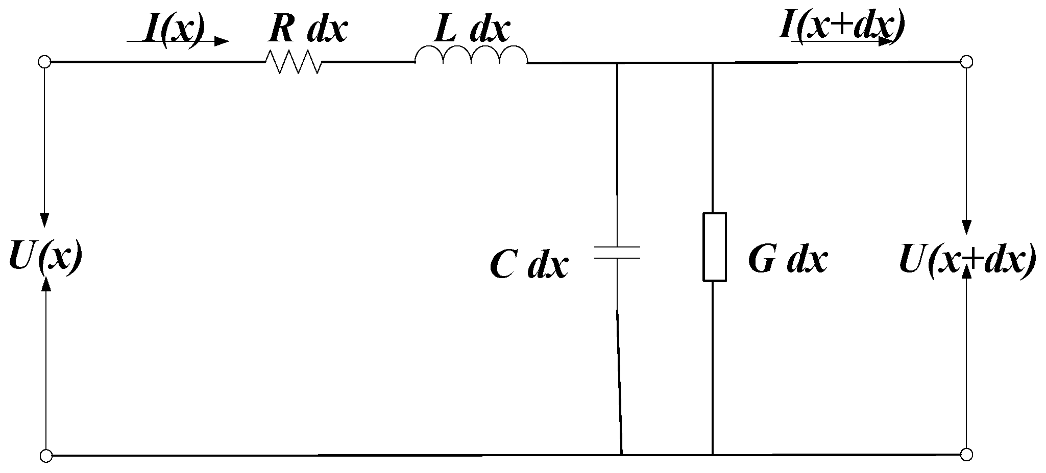
2.1. Circuit Model of a HV Cable

According to transmission line theory [23,24], a HV cable can be regarded as a distributed-parameter network consisting of series resistance-inductance (R–L) and parallel conductance-capacitance (G–C) elements along its longitudinal direction, as depicted in Figure 1.

In Figure 1, R represents resistance per unit length, L represents inductance per unit length, G represents conductance per unit length, C represents capacitance per unit length, dx represents an infinitesimal segment of the transmission line; U(x) and I(x) represent the voltage and current at position x on the transmission line, respectively; U(x + dx) and I(x + dx) represent the voltage and current at position x + dx, respectively.

Applying Kirchhoff’s laws, the governing partial differential equations describing the voltage and current distributions on the cable as a function of position x can be derived systematically.

$$\begin{array}{l}U(x)=V^{+}{e}^{-\gamma x}+V^{-}{e}^{-\gamma x}\\ I(x)={\displaystyle \frac{V^{+}{e}^{-\gamma x}-V^{-}{e}^{-\gamma x}}{Z_0}}\end{array}$$

(1)

In Equation (1), V⁺ and V⁻ represent the incident and reflected components of the electromagnetic wave, respectively. γ represents the propagation coefficient of the transmission line, and Z₀ represents the characteristic impedance, as defined in Equations (2) and (3).

$$\gamma =\sqrt{(R+j\omega L)(G+j\omega C)}=\alpha +j\beta$$

(2)

$$Z_0=\sqrt{{\displaystyle \frac{R+j\omega L}{G+j\omega C}}}$$

(3)

In Equation (2), α is the attenuation constant and β is the phase constant, which are expressed as (4).

$$\beta ={\displaystyle \frac{\omega }{v}}={\displaystyle \frac{2\pi f}{v}}$$

(4)

In Equation (4), f is the frequency and v is the wave velocity of electromagnetic waves in the cable.

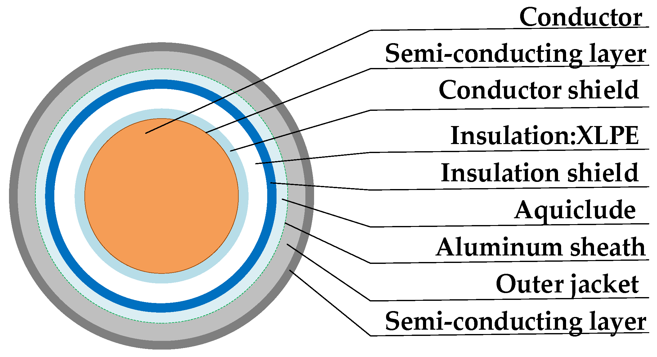
2.2. Distributed Parameters of HV Cables

HV cables are the main research object of this study. Typical HV cables adopt a single-core structure, as illustrated in Figure 2. Single-core cables are composed of a central conductor, an insulating layer, and a metal sheath, and the structure is relatively simple.

The distributed resistance is mainly determined by the conductivity of the core conductor and metal sheath, as expressed in Equation (5). The distributed inductance includes the self-inductance and mutual inductance of the core conductor and the metal sheath, as shown in Equation (6).

$$R=R_c+R_s={\displaystyle \frac{{\rho }_c}{\pi r_1^2}}+{\displaystyle \frac{{\rho }_s}{\pi (r_3^2-r_2^2)}}$$

(5)

$$L=L_c+L_s+M_{cs}={\displaystyle \frac{{\mu }_0}{8\pi }}+{\displaystyle \frac{{\mu }_0}{2\pi }}\left({\displaystyle \frac{\left(r_3^2-3r_2^2\right)}{4(r_3^2-r_2^2)}}+{\displaystyle \frac{r_2^4}{(r_3^2-r_2^2)}}\cdot \ln \left({\displaystyle \frac{r_3}{r_2}}\right)+\ln \left({\displaystyle \frac{r_3}{r_2}}\right)\right)$$

(6)

In Equation (5), R_c is the resistance of the core conductor, and R_s is the resistance of the metal sheath. ρ_c and ρ_s are the resistivities of the core conductor and the metal sheath, respectively. r₁ is the radius of the core conductor, r₂ is the outer radius of the main insulation, and r₃ is the outer radius of the metal sheath. In Equation (6), L_c represents the self-inductance of the core conductor, L_s represents the self-inductance of the metal sheath, and M_cs represents the mutual inductance between the core conductor and metal sheath.

In traditional cable modeling, the distributed admittance component usually assumes that the insulating medium is an ideal lossless dielectric, as shown in Equation (7). However, in practical applications, insulation aging can cause significant changes in the polarization and conductivity properties of the material. Particularly in cross-linked polyethylene (XLPE) insulation, thermal aging can cause microstructural changes, including chain scission and an increase in polar groups, leading to frequency-dependent dielectric dispersion. To accurately capture this phenomenon, the Cole-Cole model is used to describe the complex dielectric constant of aging XLPE, as shown in Equation (8). In polymer dielectric spectroscopy, XLPE, as a typical semi-crystalline polymer, exhibits obvious frequency-dependent dielectric relaxation behavior [25]: the low-frequency region is dominated by α relaxation (originating from the main chain segment motion) and low-frequency conductivity (mainly originating from ionic conduction and interface polarization), while the high-frequency region exhibits symmetrically broadened β relaxation (originating from the side group rotation). The symmetric broadening factor α in the Cole-Cole model directly characterizes the relaxation time distribution width of β relaxation [26,27]. This feature is consistent with the inherent heterogeneous polarization characteristics of XLPE due to its cross-linked structure.

$$G+j\omega C=j\omega {\displaystyle \frac{2\pi \epsilon }{\ln (\frac{r_2}{r_1})}}$$

(7)

$$\epsilon ={\displaystyle \frac{A{\epsilon }_0}{1+B{(j\omega )}^P}}$$

(8)

In Equation (8), ε represents the dielectric constant of the cable insulation, ε₀ represents the permittivity of vacuum, A and B are fitting constants, P corresponds to a parameter within the range of 0 to 1.

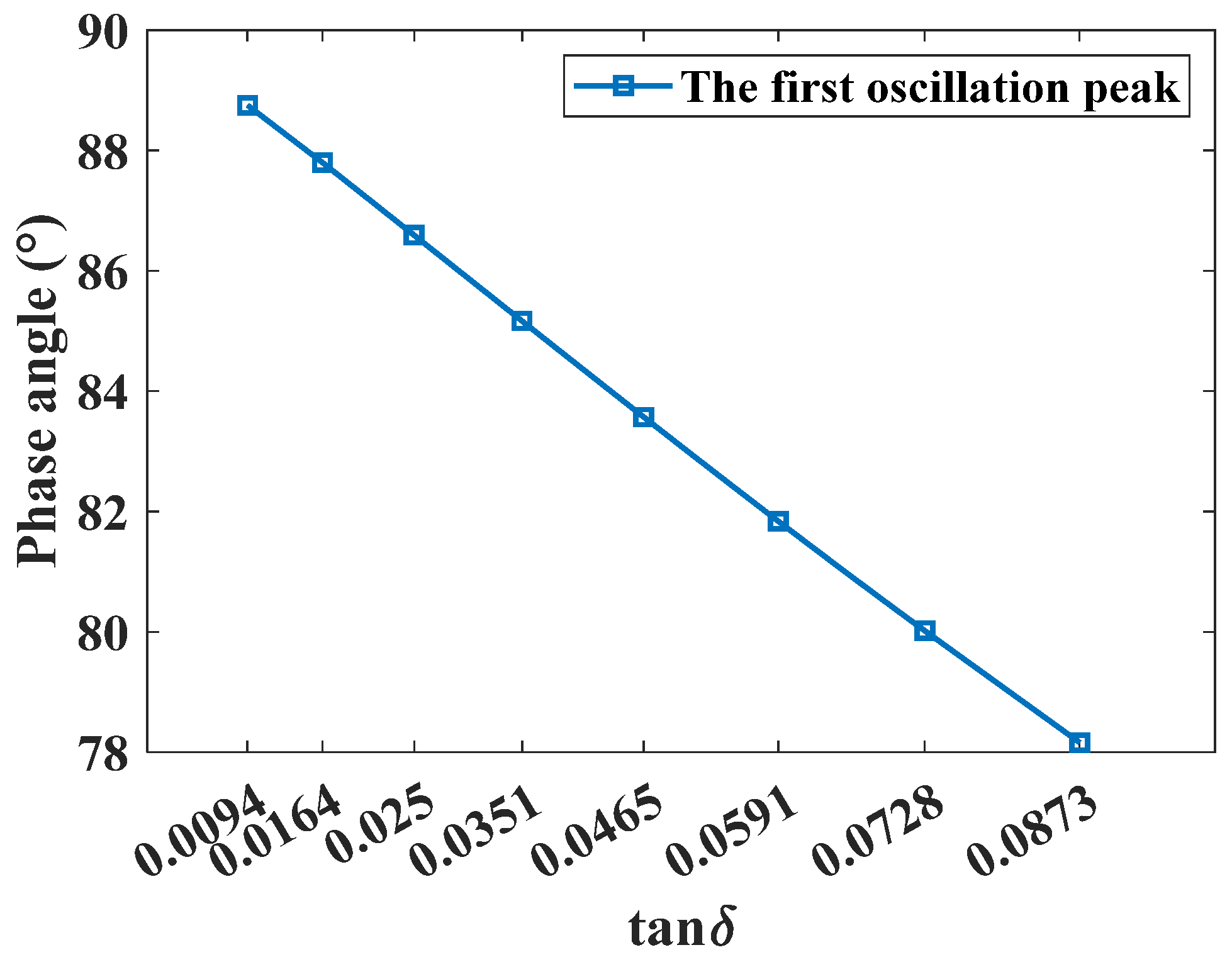
2.3. Correlation Between Dielectric Loss Tangent and Aging Condition

In the assessment of cable aging, the dielectric loss tangent (tanδ) is a key indicator for quantifying insulation degradation. Defined as the ratio of the imaginary to real parts of the complex dielectric constant, tanδ quantifies the energy dissipation characteristics of the insulating medium under the action of an alternating electric field. It essentially represents the ratio of the effective (active power) to reactive (energy storage) components of the leakage current, thus helping to understand insulation integrity and aging severity.

$$\tan \delta ={\displaystyle \frac{\mathrm{The} \mathrm{energy} \mathrm{lost} \mathrm{by} \mathrm{the} \mathrm{medium}}{\mathrm{The} \mathrm{energy} \mathrm{stored} \mathrm{in} \mathrm{the} \mathrm{medium}}}$$

(9)

In cable insulation materials, aging mechanisms typically involve molecular chain breakage, the formation of polar groups, and the development of microstructural defects. These physicochemical changes can lead to significant changes in the dielectric loss properties of the material. Empirical studies have shown that thermal aging, oxidative degradation, and partial discharge damage can lead to significant increases in dielectric loss values. Moreover, the extent of this increase is closely related to the severity of insulation aging [28,29,30], especially in XLPE and other polymer-insulated cables.

2.4. Input Impedance at the Source End of the Localized Aging Cable

As derived in Equation (1), the input impedance of the cable at position x adheres to the analytical expression presented in Equation (10).

$$Z(x)={\displaystyle \frac{U(x)}{I(x)}}=Z_0{\displaystyle \frac{1+\Gamma e^{-2\gamma x}}{1-\Gamma e^{-2\gamma x}}}$$

(10)

In Equation (10), Γ represents the reflection coefficient of the cable, defined as Equation (11), where Z_L is the load impedance of the cable.

$$\Gamma ={\displaystyle \frac{Z_L-Z_0}{Z_L+Z_0}}$$

(11)

To examine the effects of localized aging, a three-segment cable model is constructed, as shown in Figure 3. Although the aging segments share the same dimensions as the healthy ones, the degradation of dielectric properties leads to distinct electromagnetic behavior. Aging alters the molecular structure and polarization characteristics of the insulating material, thereby affecting its ability to store electric field energy, and aging increases the loss of converting electrical energy into heat energy under an alternating electric field. These changes result in variations in the dielectric constant and dielectric loss factor, causing the aging segment to exhibit different propagation constants and characteristic impedances compared to the adjacent healthy segment. The model includes a healthy segment at the source end, an aging segment in the middle, and a healthy segment at the end. The boundaries of the aging segment defined by spatial coordinates l_a and l_b. A layer-by-layer recursive algorithm based on transmission line theory is used to calculate the impedance of the source end through inverse analysis.

Under the open-circuit boundary condition where the terminal load impedance is infinite, that is, the reflection coefficient is equal to 1, the input impedance Z_b of the healthy segment at the boundary l_b can be obtained by Equation (12). This impedance is used as the terminal load of the adjacent aging segment, and the modified reflection coefficient formula in Equation (13) is used to derive the analytical expression of the input impedance Z_a at the boundary l_a. Subsequently, using Z_a as the terminal load of the first healthy segment and applying the reflection coefficient defined in Equation (14), the theoretical impedance of the cable source end can be determined, as shown in Equation (15).

$$Z_b=Z_{0h}{\displaystyle \frac{1+e^{2{\gamma }_b(l_b-l)}}{1-e^{2{\gamma }_b(l_b-l)}}}$$

(12)

$${\Gamma }_d={\displaystyle \frac{Z_b-Z_{0d}}{Z_b+Z_{0d}}}$$

(13)

$${\Gamma }_h={\displaystyle \frac{Z_a-Z_{0h}}{Z_a+Z_{0h}}}$$

(14)

$$Z_{in}=Z_{0h}{\displaystyle \frac{1+{\Gamma }_h{e}^{-2{\gamma }_h{l}_a}}{1-{\Gamma }_h{e}^{-2{\gamma }_h{l}_a}}}$$

(15)

The relevant propagation, reflection, and characteristic impedance parameters are defined as follows: γ_h and γ_d represent the propagation coefficients of the healthy and aging segments, respectively; Γ_h and Γ_d represent the reflection coefficients at the boundaries of the healthy segment and the aging segment, respectively; while Z_0h and Z_0d represent the characteristic impedances of the healthy and aging segments, respectively.

3. Simulation and Analysis

3.1. Background of Simulation

In this study, the YJLW03-110kV-1*630 XLPE insulated power cable was selected as the specific research object. As illustrated in Figure 2, the cable features a multi-layer coaxial structure, including copper conductor, XLPE insulation, metal sheath, and polyethylene jacket. The geometric structure and material properties of the cable are summarized in

Table 2. Basic structural and material parameters of the object cable.

Structure	Radius/Thickness (mm)
Conductor	14.9
Semi-conducting layer	2
Insulation	16.5
Aquiclude	2
Aluminum sheath	2
Outer jacket	4

, and

Table 3. Geometric parameters for YJLW03-110kV-1*630 type cable.

Parameters Related to Impedance Spectroscopy	Value
r1	14.9 mm
r2	35.4 mm
r3	41.4 mm
ρc	1.68 × 10−8 (Ω·m)
ρs	2.83 × 10−8 (Ω·m)

lists the key parameters used to derive the impedance spectroscopy in detail.

3.2. Simulation and Results

3.2.1. Impedance Spectroscopy of Cables Under Different Conditions

The impedance spectroscopy characteristics of a 500-m HV single-core cable under different aging conditions under open circuit conditions were simulated. The scanning frequency range is 100 kHz to 3.5 MHz. The complex dielectric constant fitting coefficients are: A = 2.68, B = 0.14, P = 0.02 for the original healthy cable; A = 4.26, B = 0.22, P = 0.05 for the aging cables [31]. To compare the differences in cable impedance spectroscopy under different conditions, three representative conditions (healthy insulation, overall aging, and localized aging) were simulated, as shown in Figure 4.

As shown in Figure 4, the impedance amplitude spectroscopy of a healthy cable presents a periodic pulse shape, while the corresponding phase spectroscopy presents a periodic oscillation. Under overall aging, the basic characteristics of the impedance spectroscopy remain unchanged, but both the amplitude spectroscopy and the phase spectroscopy will systematically shift to the low-frequency region. In contrast, the overall change of the impedance spectroscopy caused by localized aging is relatively small. The slight change in the amplitude spectroscopy occurs at the resonance peak. In the phase spectroscopy, localized aging mainly causes slight deviations at the zero-crossing frequency. These localized changes will be further analyzed in the next section.

Based on the aging model established in this paper, the complex dielectric constant ε in Equation (7) is replaced by the general formula shown in Equation (16).

$$\epsilon ={\epsilon }^{\prime }-j{\epsilon }^{″}$$

(16)

In Equation (16), ε′ is the real part of the complex permittivity, representing the material’s ability to store electric field energy, while ε″ is the imaginary part of the complex permittivity, which reflects the material’s energy dissipation under an electric field. Substitution of Equation (16) into Equation (7) yields the expressions for G and C as Equation (17).

$$\begin{array}{l}G=\omega {\displaystyle \frac{2\pi {\epsilon }^{″}}{\ln (r_2/r_1)}}\\ C=\omega {\displaystyle \frac{2\pi {\epsilon }^{\prime }}{\ln (r_2/r_1)}}\end{array}$$

(17)

Therefore, in the aging condition simulated in Figure 4, as the real part of the complex permittivity increases, the distributed capacitance value also increases. Since the resonance frequency in the impedance amplitude spectroscopy is mainly determined by the wave velocity [32], and the wave velocity in the cable is approximately Equation (18), the resonance frequency can be calculated by Equation (19).

$$v={\displaystyle \frac{1}{\sqrt{LC}}}$$

(18)

$$f={\displaystyle \frac{nv}{2l}}(n=1,2,3,\dots )$$

(19)

In Equation (19), v is the wave velocity, l is the cable length, and n is the harmonic order.

Due to aging, the distributed capacitance increases, leading to a decrease in the resonance frequencies. Under overall aging condition, the entire impedance amplitude spectroscopy moves toward the low frequency direction; under localized aging conditions, the resonance peak frequency in the impedance amplitude spectroscopy decreases. Meanwhile, the amplitude of the impedance resonance peaks is mainly affected by loss, including conductor loss (R) and dielectric loss (G). Near the resonance frequency, under low-loss conditions, the impedance amplitude can be approximated by Equation (20), where α is approximated as $\surd$RG.

$$\left|Z_{in}\right|\approx {\displaystyle \frac{Z_0}{\alpha l}}$$

(20)

Thus, when G increases, the attenuation constant α increases, leading to a decrease in the amplitude of the impedance.

3.2.2. Influence of Overall Aging on Impedance Spectroscopy

The overall aging cable impedance spectroscopy under different aging severity levels were simulated, as shown in Figure 5. The selected tanδ range is 0.0094–0.0873, which systematically covers the complete aging spectroscopy of XLPE insulation, from incipient degradation to critical failure state [33].

As shown in Figure 5, with the aging intensifies, the resonance peak in the amplitude spectroscopy and the oscillation peak in the phase spectroscopy both show a significant downward trend, and the entire impedance spectroscopy moves toward the low frequency direction. It is worth noting that in Figure 5b, the peak value of the first oscillation peak of the phase spectroscopy gradually decreases with the increase of aging degree, and this trend is further reflected in Figure 6. Therefore, this characteristic parameter can be used as an effective quantitative indicator to assess the overall aging severity of HV cables.

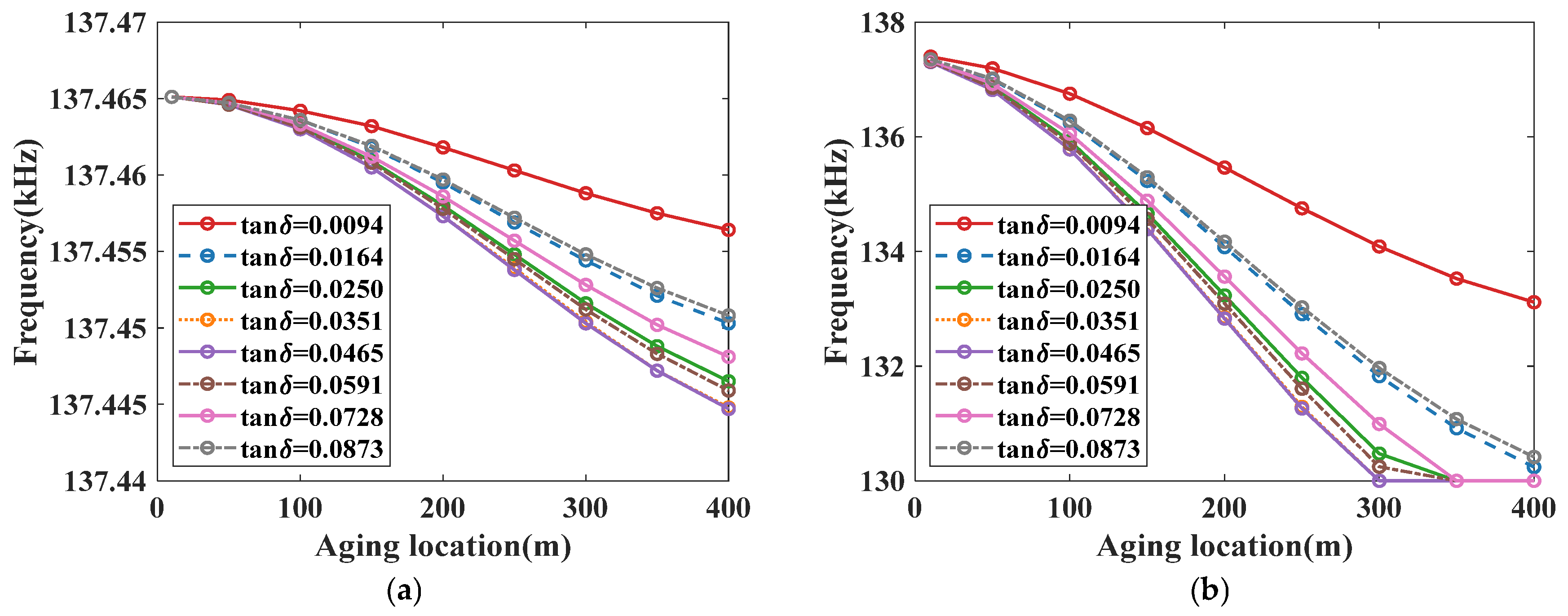
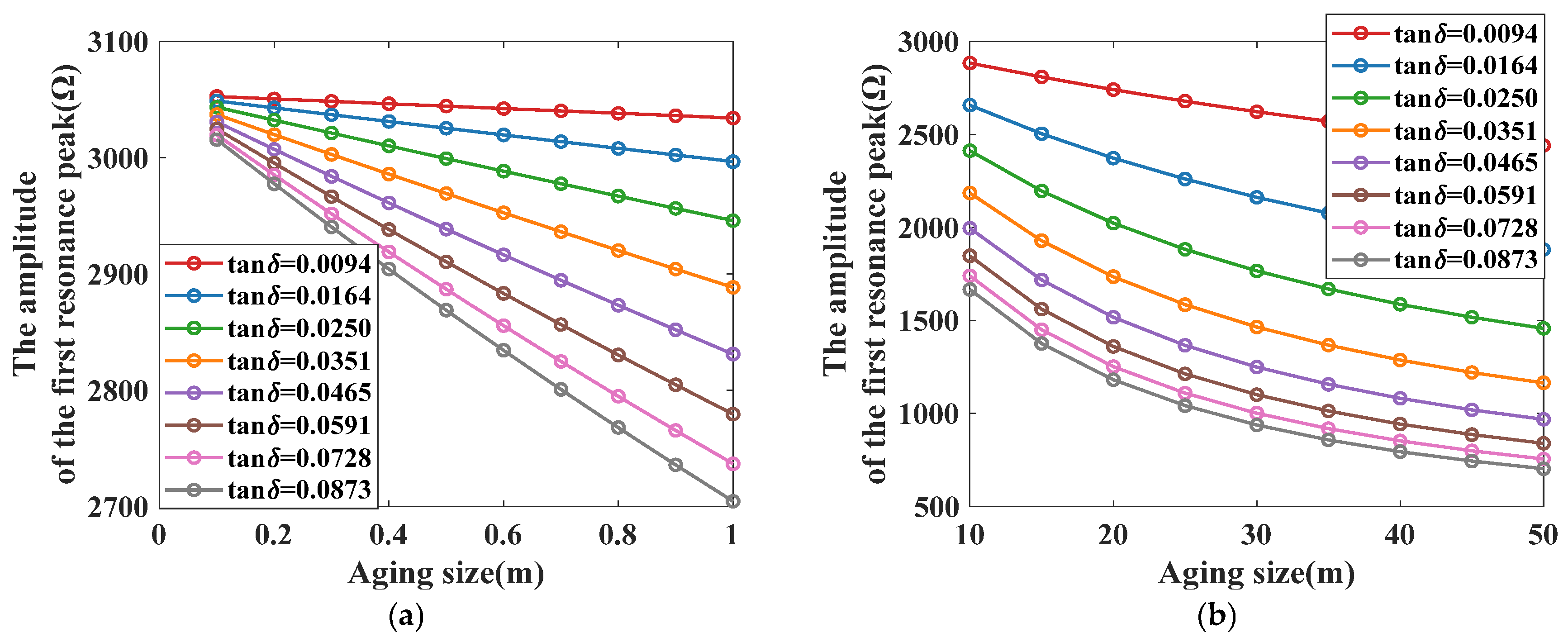
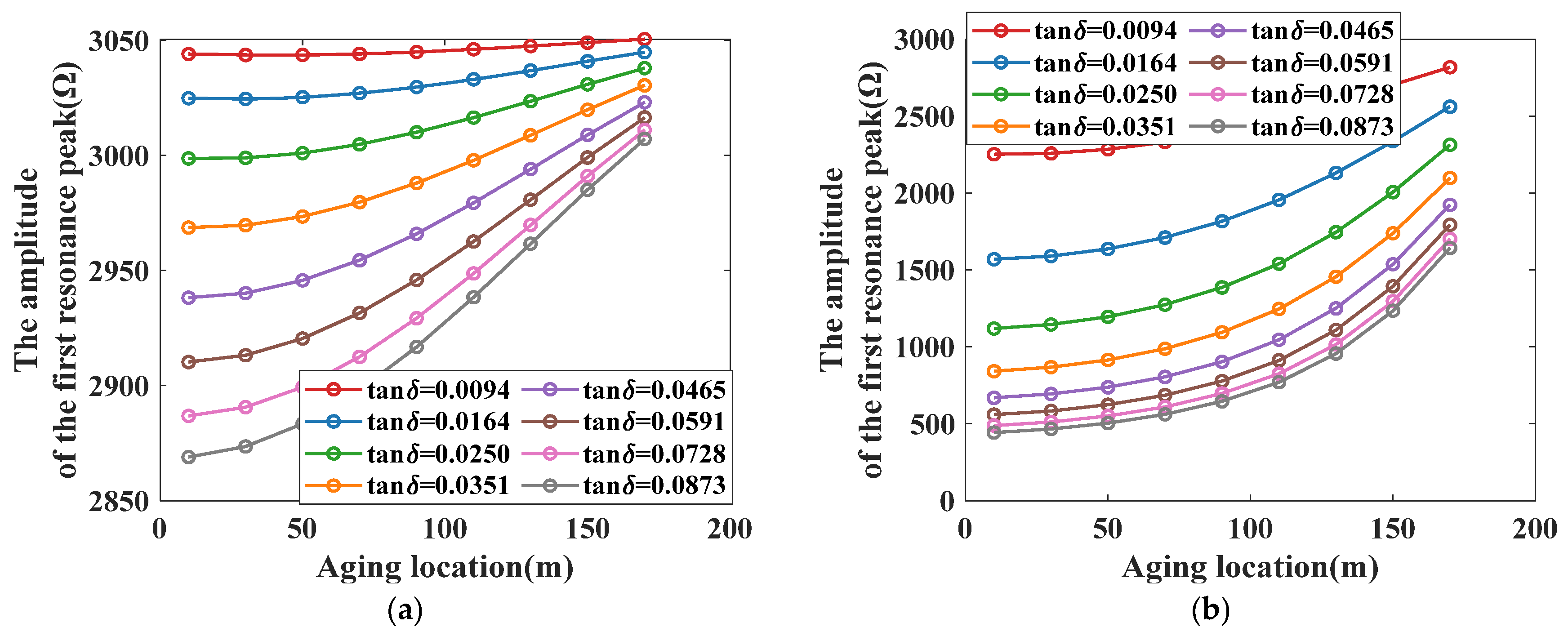
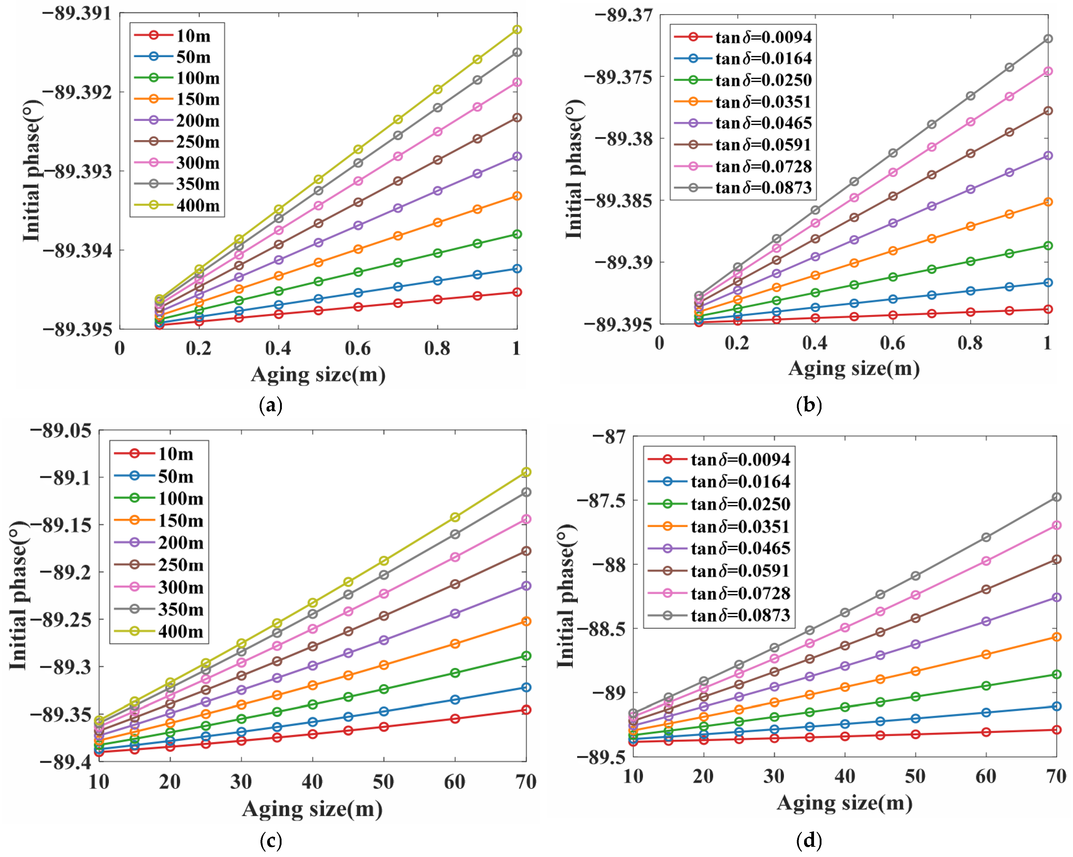
3.2.3. Influence of Localized Aging on the Impedance Spectroscopy

To specifically investigate the influence of localized aging on impedance spectroscopy characteristics, the relative variation rates of impedance amplitude and phase under two different localized aging conditions were calculated by Equation (21), with reference to the baseline parameters of healthy cables.

$$\begin{array}{l}\Delta {\left|\mathit{Z}\right|}_{\mathit{r}\mathit{e}\mathit{l}}={\displaystyle \frac{\left|{\mathit{Z}}_{\mathit{a}\mathit{g}\mathit{i}\mathit{n}\mathit{g}}(\mathit{f})\right|-\left|{\mathit{Z}}_{\mathit{b}\mathit{a}\mathit{s}\mathit{e}}(\mathit{f})\right|}{\left|{\mathit{Z}}_{\mathit{b}\mathit{a}\mathit{s}\mathit{e}}(\mathit{f})\right|}}\times 100\%\\ \Delta {\mathit{\theta }}_{\mathit{r}\mathit{e}\mathit{l}}={\displaystyle \frac{{\mathit{\theta }}_{\mathit{a}\mathit{g}\mathit{i}\mathit{n}\mathit{g}}(\mathit{f})-{\mathit{\theta }}_{\mathit{b}\mathit{a}\mathit{s}\mathit{e}}(\mathit{f})}{{\mathit{\theta }}_{\mathit{b}\mathit{a}\mathit{s}\mathit{e}}(\mathit{f})}}\times 100\%\end{array}$$

(21)

In Equation (21), |Z_base(f)| and θ_base (f) represents the impedance amplitude and phase of the healthy reference cable respectively, while |Z_aging(f)| and θ_aging (f) denotes those of the aging cables, Δ|Z|_rel and Δθ_rel represent the impedance amplitude and phase change rates of the aging cables relative to the healthy reference cable. It should be emphasized that both aging conditions maintained identical aging severity and spatial location, differing solely in the size of localized aging region—Condition 2 (Size: 50 m) encompassing a larger aging size than Condition 1 (Size: 1 m), the comparison are illustrated in Figure 7.

As shown in Figure 7a, the resonance peaks in the amplitude spectroscopy show obvious changes caused by aging. Specifically, the relative amplitude variation rates (Δ|Z|_rel) near these resonance peaks exceed 0.3% under Condition 1 and exceed 13% under Condition 2. Similarly, the phase spectroscopy analysis shows that the sensitivity to insulation degradation is enhanced near the phase angle zero crossing in Figure 7b, where the phase variation rates (Δθ_rel) exceed 0.6% and 27% under Conditions 1 and 2, respectively. Quantitative analysis confirms that phase spectroscopy parameters are more responsive to localized aging than amplitude-based metrics. Under the same localized aging conditions, the sensitivity of the phase spectroscopy to the frequency domain response of localized aging is more than twice that of the amplitude spectroscopy. These results emphasize the feature recognition ability of the phase spectroscopy in diagnosing the insulation condition of cables and lay the foundation for the development of a phase-frequency characteristic-based diagnostic method for cable insulation aging assessment.

Building on these findings, the diagnostic indicators for cable insulation conditions are investigated through three critical parameters: aging severity, aging location, and aging size. First, the influence of different aging sizes on the impedance spectroscopy was evaluated through simulation. The aging location was fixed at 100 m from the cable source end, and the aging size range was 1 to 50 m, as shown in Figure 8.

As shown in Figure 8, when the aging size is relatively small, the impedance spectroscopy largely adheres to the spectral evolution pattern observed in healthy cables, primarily characterized by the attenuation of resonance peak amplitudes and frequency shifts in the phase response. However, as the aging size increases, abrupt variations emerge in the resonance peak amplitudes within the impedance amplitude spectroscopy. Accordingly, localized aging conditions exhibiting abrupt jumps in the resonance peak amplitudes of the impedance amplitude spectroscopy are categorized as large-size aging condition, whereas those without such discontinuities are classified as small-size aging condition.

To further explore the diagnostic potential of the phase spectroscopy, taking large-size aging as a representative. Different aging sizes, spatial locations and severity were simulated to investigate the relationship between the aging condition and the first zero-crossing frequency of the phase, as shown in Figure 9.

As shown in Figure 9a,b, there is a significant monotonic correlation between the zero-crossing frequency value and the aging size and spatial location of localized aging. Further analysis shows that the evolution of this feature at different aging levels shows a biphasic (non-monotonic) trend, as shown in Figure 9c: as aging progresses, the zero-crossing frequency first decreases (moves to low frequency) and then increases (transitions to high frequency). In order to verify the diagnostic utility of this diagnostic parameter for localized aging, its universality is further explored by evaluating its response to changes in aging position.

To further evaluate the applicability and sensitivity of the first zero-crossing frequency as a diagnostic indicator, the study investigates its dependence on aging location under different aging sizes. Specifically, the relationship between the first phase angle zero-crossing frequency in impedance spectroscopy and the spatial location under different aging sizes is examined. By simulating frequency responses at aging sizes ranging from 0.1 m to 1.0 m (small-size aging) and 10 m to 70 m (large-size aging), the variations in this characteristic frequency parameter were systematically analyzed, as illustrated in Figure 10.

As shown in Figure 10a,b, regardless of whether the localized aging size is large or small, as the aging position approaches the cable terminal, the first phase angle zero-crossing frequency continues to move toward the low frequency direction. In addition, when the aging location is constant, as the aging size increases, the zero-crossing frequency further decreases, while the monotonic relationship between the aging location and the zero-crossing frequency remains unchanged. These results verify the diagnostic capability of the first phase angle zero-crossing frequency, demonstrating that this parameter is a reliable basis for comprehensively evaluating localized aging condition of HV cables.

Next, in order to investigate the relationship between the first phase angle zero-crossing frequency and the aging severity under different aging conditions, the cable insulation with tanδ ranging from 0.0094 to 0.0873 was numerically simulated, and the first phase angle zero-crossing frequency values with aging sizes of 0.1 m and 50 m were evaluated, as shown in Figure 11.

As illustrated in Figure 11, the first phase angle zero-crossing frequency parameter exhibits limited resolution in the investigated aging range regardless of the aging location. The limited sensitivity of this parameter to variations in aging severity underscores its inadequacy for quantitative assessment of degradation extent. These findings emphasize the necessity of introducing complementary diagnostic indicators to enable accurate evaluation of localized insulation aging in HV cables.

It is worth noting that variations in localized aging severity result in pronounced changes in the amplitude of the first resonance peak in the impedance amplitude spectroscopy. In order to clarify the correlation between this peak feature and the aging severity, the relationship between the two at different aging severity was studied. Specifically, the cable insulation with a tanδ range of 0.0094–0.0873 was simulated, and the changes in peak parameters when the aging size range was 0.1–1.0 m (small-size) and 10–50 m (large-size) were analyzed, as shown in Figure 12. At the same time, a parameter study was conducted to characterize the evolution of the peak parameters at the aging location of 10–170 m in the same dielectric loss range (0.0094–0.0873), and the corresponding results are shown in Figure 13.

As shown in Figure 12, when the aging size is constant, the peak parameter gradually decreases with increasing aging severity. Similarly, as shown in Figure 13, when the aging location is constant, the peak parameter shows a consistent decreasing trend with the increase of aging severity. These results confirm that the amplitude of the first resonance peak in the impedance amplitude spectroscopy can be used as a key supplementary indicator to characterize the localized aging process of cable insulation. This parameter effectively solves the diagnostic limitations of single-frequency indicators and improves the overall sensitivity and reliability of aging assessment.

Next, in order to establish a more comprehensive evaluation standard for the localized aging condition of cable insulation, a new supplementary indicator, the initial phase of cable impedance, is introduced. The changes in the initial phase at different aging positions (ranging from 10 m to 400 m) and the changes in the localized aging dielectric loss value of 0.0094–0.0873 were simulated, as shown in Figure 14.

As shown in Figure 14a,b, under small-size aging conditions (0.1–1.0 m), the initial phase gradually increases with the increase of the aging size; in addition, when the localized aging location is determined, the change in aging severity does not change the monotonic relationship between the initial phase and the aging size. Similarly, in Figure 14a,b, this relationship remains unchanged under large-size aging conditions (10–70 m). These results confirm the universality of the initial phase parameter and support its use as a supplementary indicator for quantitatively assessing the localized aging size of cable insulation.

3.2.4. Impedance Spectroscopy-Based Diagnostic Framework for Assessing the Insulation Condition of HV Single-Core Cables

Building upon the previous analysis of impedance spectroscopy characteristics at the source end of cable under various aging conditions, a diagnostic method for assessing the insulation aging conditions of HV single-core cables is proposed, as shown in Figure 15.

Step 1: For a HV single-core cable with unknown insulation health condition, obtain the reference impedance spectroscopy corresponding to the healthy condition according to the cable design specifications. Compare the measured impedance spectroscopy of the test cable with the reference to generate a change rate comparison plot. If no abrupt changes are observed in this plot, the insulation is considered to be in a healthy condition. If variations are detected, proceed to step 2.

Step 2: Inspect the amplitude spectroscopy of the test cable. If the amplitudes of the resonance peak in the spectroscopy don’t monotonically decrease, this indicates a large-size localized aging condition. In such cases, move to step 4 for localized aging diagnosis. If the amplitudes of the resonance peak monotonically decrease, proceed to step 3.

Step 3: Analyze the phase spectroscopy of the test cable. The monotonically decreasing oscillation peak of the phase spectroscopy indicates overall aging, and the severity of insulation degradation can be quantified by the first oscillation peak in the impedance phase spectroscopy. Specifically, the more severe the insulation aging, the lower the amplitude of the first oscillation peak in the phase spectroscopy. Conversely, if the oscillation peak in the phase spectroscopy is not monotonically decreasing, it implies small-size localized aging condition. Then, proceed to Step 4 to diagnose the localized aging condition.

Step 4: Determine localized aging parameters: aging size, aging severity and aging location. A systematic multi-parameter diagnostic method for localized aging characterization is established in the study. The analysis in the previous section showed that the first phase angle zero crossing has limited sensitivity to changes in the severity of localized insulation aging. Therefore, this parameter can be used to determine the size and location of localized aging without prior knowledge of the aging severity. In addition, it was found that an increase in the aging size causes the first phase zero crossing to move monotonically to low frequencies, while the initial phase increases with the increase in the aging size. Therefore, the aging size can be accurately determined by combining the first phase angle zero crossing and the initial phase in the impedance phase spectroscopy. Subsequently, the amplitude of the first resonance peak in the impedance spectroscopy can be used as an effective indicator for evaluating the severity of aging, where the more obvious the insulation degradation, the smaller the resonance peak amplitude. Finally, with the predetermined aging size and severity as input, the precise location of localized aging can be achieved by analyzing the first zero crossing frequency, which shows a decreasing trend as the aging location moves away from the cable source end.

3.3. Analysis of Factors Influencing the Impedance Spectroscopy

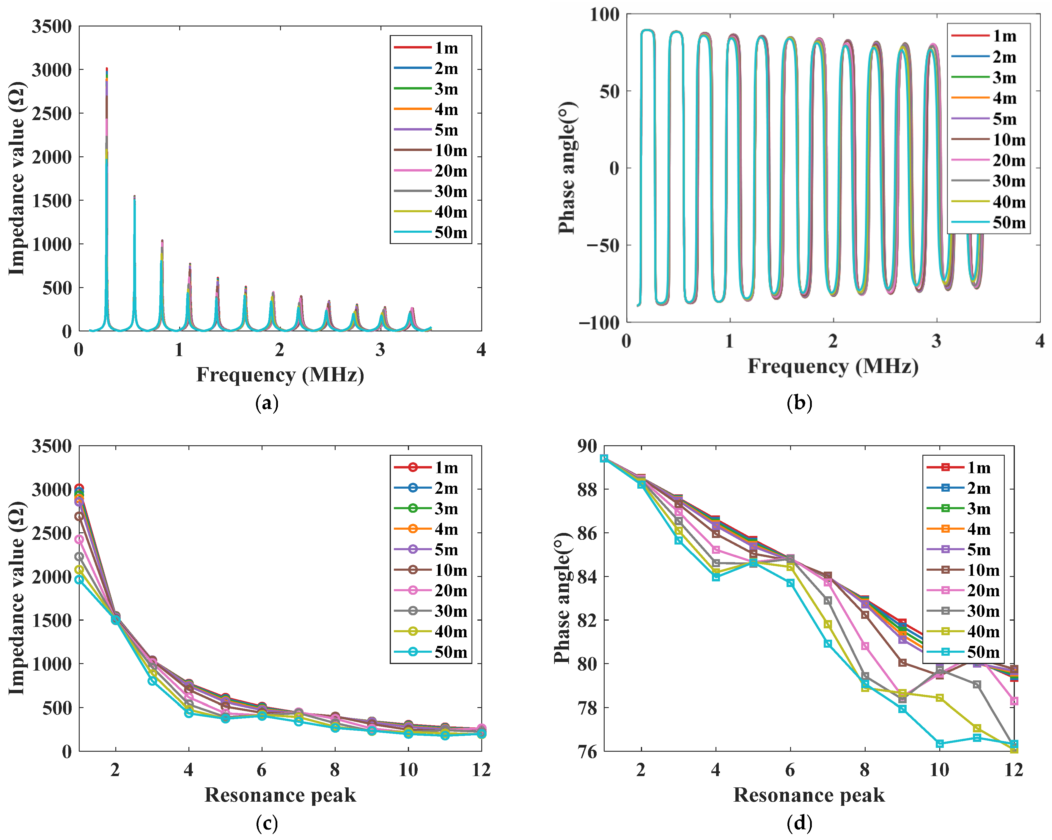
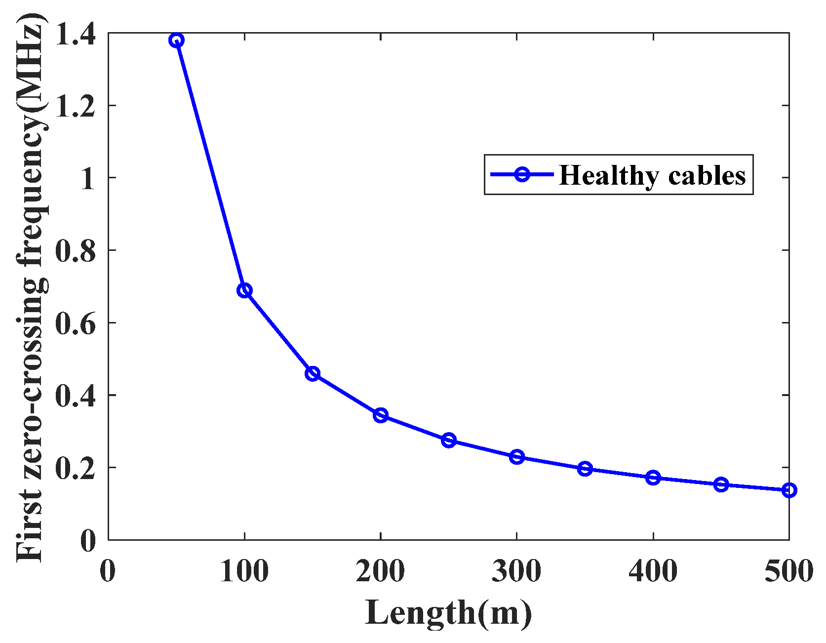
3.3.1. Impact of Cable Length

Cable length is a critical parameter influencing impedance spectroscopy measurements. According to Equation (19), cable length directly determines the spacing of the resonance peaks in the amplitude spectroscopy and the oscillation period in the phase spectroscopy. This theoretical relationship implies that variations in cable length fundamentally alter the frequency response characteristics of the impedance spectroscopy. To validate this principle, simulations were conducted to evaluate the variation in the first zero-crossing frequency (as a characteristic point) across cable lengths ranging from 50 m to 500 m, as illustrated in Figure 16.

As shown in Figure 16, as the cable length increases, the characteristic points in the impedance spectroscopy shift toward the low frequency direction. This phenomenon confirms that for cables with the same conditions, the characteristics in their impedance spectroscopy (such as resonance peaks, zero crossings, etc.) will change with the length. Consequently, cable length must be accounted for when comparing the impedance spectroscopic characteristics across different cable segments or installations.

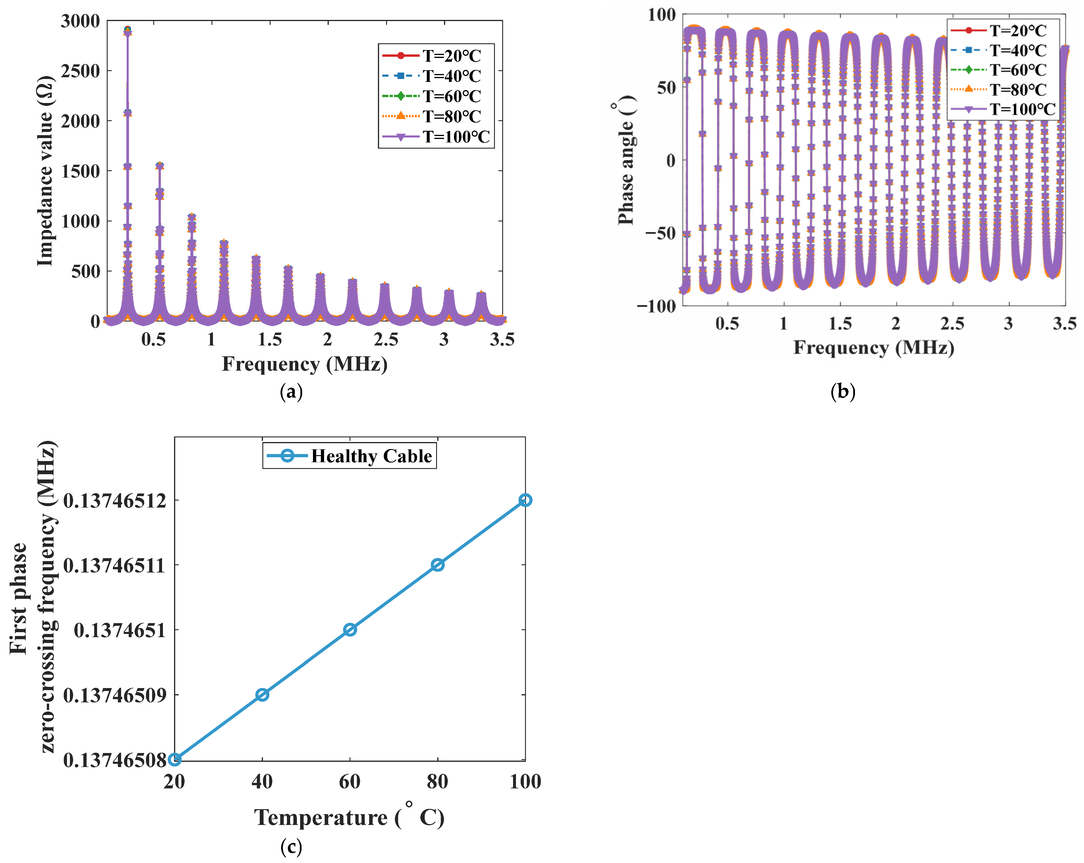
3.3.2. Impact of Instantaneous Temperature

When evaluating the insulation condition of HV single-core cables, temperature, as the primary source of thermal stress, affects insulation performance through both long-term cumulative effects and short-term transient disturbances. Long-term exposure to high temperatures can cause irreversible changes in the chemical structure of XLPE insulation through mechanisms such as thermal oxidation and cross-link bond breakage. This gradual degradation process represents the inherent characteristics of insulation degradation captured by the proposed method.

Over the timescale of a single impedance spectroscopy measurement, the microstructural changes caused by thermal aging can be regarded as a steady-state background. Under these conditions, ambient temperature fluctuations mainly introduce interference through transient thermal effects, which are mechanistically distinct from long-term thermal degradation. As noted in Equation (22), rapid temperature fluctuations during measurement predominantly affect the conductor resistance of the cable, constituting the most immediate and pronounced source of disturbance.

$$\rho ={\rho }_{20}\cdot (1+\alpha (T-20))$$

(22)

In Equation (22), ρ represents the conductor resistivity, ρ₂₀ represents the conductor resistivity at 20 °C, α is the conductor’s temperature coefficient of resistance, and T represents the ambient temperature.

Accordingly, the impedance spectroscopy of the cable source end of a healthy cable was simulated under ambient temperatures ranging from 20 °C to 100 °C, as illustrated in Figure 17.

As shown in Figure 17, the influence of temperature increase on the impedance spectroscopy curve is almost negligible. Specifically, the effect on the first phase angle zero-crossing frequency is limited to approximately 0.01 μHz. If higher accuracy is required in actual applications, a correction term can be introduced to consider the effect of ambient temperature on the conductor resistivity.

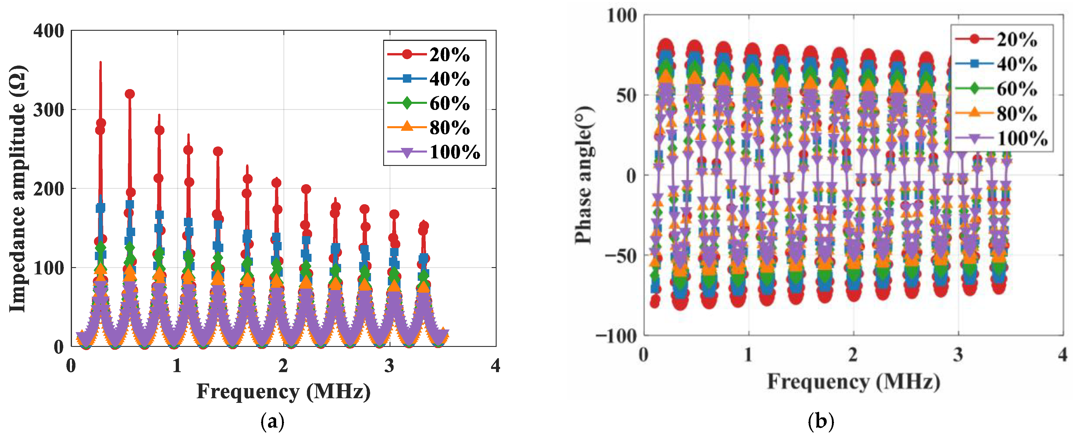
3.3.3. Impact of Load Rate

The load rate of a cable is defined as the ratio of its actual transmitted current to its rated current carrying capacity. By adjusting the terminal load, the cable impedance spectroscopy with load rate ranging from 20% to 100% was simulated, as illustrated in Figure 18.

As shown in Figure 18, as the cable load rate increases, the impedance amplitude and phase decrease, and the steepness of the amplitude spectroscopy decreases significantly. This characteristic can be used as a key indicator to assess the current load level of the cable. Accordingly, during the cable impedance spectroscopy test and condition assessment, the actual load rate must be considered and recorded. Variations in the resonance peaks in the impedance spectroscopy (including trends and values) can be used to determine and calibrate the load level, thereby reducing the impact of load fluctuations on the diagnostic results.

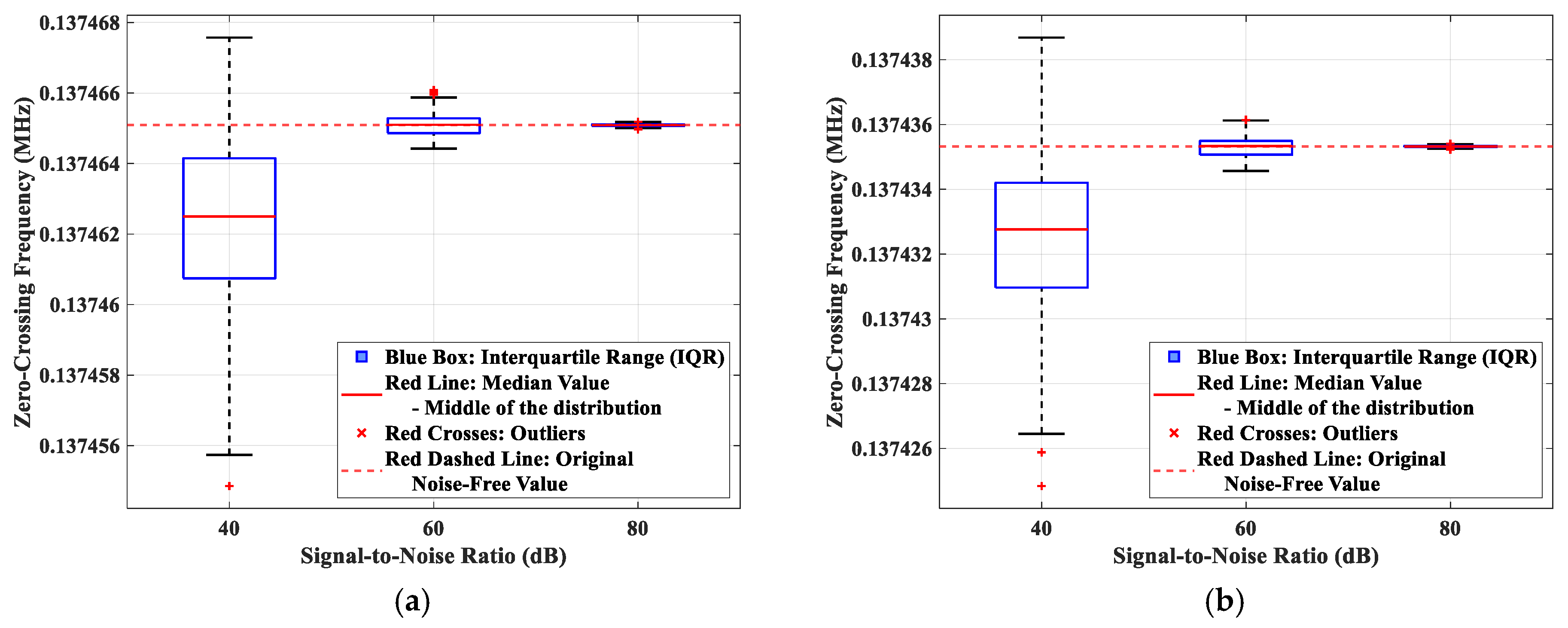
3.4. Sensitivity Analysis of the Proposed Method to Random Noise

In order to verify the robustness of the proposed method under noisy conditions, this section evaluates the impact of random noise on the detection of the impedance phase angle zero-crossing frequency through sensitivity analysis. The noise sensitivity analysis is conducted within a Monte Carlo simulation framework [34]. The noise model is constructed by superimposing complex Gaussian white noise onto the simulated impedance spectroscopy [35,36], as described in Equation (23).

$$Z_{noisy}=Z_{true}+{\mathcal{N}}_{real}+j{\mathcal{N}}_{imag}$$

(23)

In Equation (23), Z_noisy represents the noise-contaminated impedance at the source end of cable, Z_true represents the original impedance of the cable, and the real-part noise N_real and imaginary-part noise N_imag are independently Gaussian-distributed, as expressed in Equation (24).

$$\mathcal{N}~\mathcal{N}\left(0,{\sigma }^2\right), \sigma ={\displaystyle \frac{\left|Z_{true}\right|}{{10}^{\mathrm{SNR}/20}}}$$

(24)

In Equation (24), σ represents the noise standard deviation, proportional to the impedance amplitude; SNR represents the signal-to-noise ratio, indicating the signal quality. The SNR follows the standard engineering practice, as defined in Equation (25).

$$\mathrm{SNR}=20{\log }_{10}\left({\displaystyle \frac{\left|Z_{true}\right|}{\sigma }}\right)$$

(25)

Three SNR levels—40 dB, 60 dB, and 80 dB—are used here to cover typical measurement environments in industrial settings [37]. The statistical distribution of the first phase angle zero-crossing frequency under these SNR conditions was simulated, as shown in Figure 19.

In Figure 19a, the zero-crossing frequency characteristics of the healthy cable exhibits strong resistance to noise. In a low-noise environment (80 dB), the height of the box is significantly reduced, and the center line almost coincides with the original value. Under typical industrial noise conditions (60 dB), although the height of the box increases slightly, it remains compact (interquartile range, IQR < 0.000 001 MHz), the offset of the center line relative to the original value is less than 0.000 001 MHz, and the proportion of outliers is less than 0.6%, all within a reasonable range. In a high-noise environment (40 dB), the box size increases significantly, but the frequency distribution range is still between 0.137 46 MHz and 0.137 465 MHz. Similarly, as shown in Figure 19b, the localized aging cable a demonstrates comparable noise resilience under both 80 dB and 60 dB SNR conditions.

In conclusion, under typical industrial noise levels (60 dB SNR), the first zero-crossing frequency in the phase spectroscopy demonstrates robust resistance to noise interference.

4. Discussion

4.1. The Cause of the Dual-Frequency Offset Phenomenon

As mentioned in Section 3, within the aging range considered in this study, the first phase angle zero-crossing frequency of the localized aging cable exhibits a characteristic dual-frequency migration pattern (first moving to low frequency and then to high frequency), as shown in Figure 9c. In order to explore the underlying mechanism of this phenomenon, the correlation between the zero-crossing frequency and the aging severity under different aging sizes and locations is systematically investigated, taking large-size localized aging as a representative, as shown in Figure 20.

As shown in Figure 20, bidirectional frequency migration is prevalent within the defined aging severity range. In the proposed cable aging model, the admittance component in the distributed transmission line parameters is mainly affected by insulation degradation. The impedance spectroscopy is a mathematical representation of the inherent wave propagation characteristics, where the theoretical expression of the first phase angle zero-crossing frequency is derived from Equation (19) as shown in Equation (26), where l is the cable length, L is the cable inductance per unit length, and C is the cable capacitance per unit length.

$$f\approx {\displaystyle \frac{1}{4l\sqrt{LC}}}$$

(26)

In Equation (26), the first phase angle zero-crossing frequency is inversely proportional to the change in the insulation capacitance value. According to the aging model used in the study, the insulation capacitance first increases and then decreases within the studied aging severity. Therefore, as the aging severity intensifies, the frequency first moves toward the low frequency direction and then moves toward the high frequency direction.

4.2. Comparison

In this section, the proposed method is compared with conventional insulation condition assessment methods, with the comparison results presented in

Table 4. Comparison of insulation condition diagnostic methods.

Method	The Proposed Method	Traditional Electrical Test	Partial Discharge (PD)
Dimension
Detection principle	Impedance spectroscopy	Insulation resistance	Partial discharge signal
Non-destructiveness	Excellent	Moderate	Good
Condition discrimination	Excellent (Healthy/Overall/Localized)	Poor	Excellent
Sensitivity to localized aging	Excellent	Poor	Excellent
Quantification of overall aging	Good	-	-
Robustness	Excellent	Moderate	Moderate
Convenience	Excellent	Moderate	Poor
Cost-effectiveness	Good	Moderate	Poor

. Taking insulation resistance testing as an example, traditional electrical testing methods [38] are somewhat invasive and cannot distinguish between overall aging and localized aging, nor can they provide information to quantify the severity of overall aging. Although the equipment required for these methods is relatively common and cost-effective, the testing process is highly susceptible to environmental conditions. The test system of partial discharge (PD) detection technology is relatively complex [39], including multiple components such as sensors, acquisition units, and positioning systems. This complexity leads to high testing costs, poor testing convenience, and susceptibility to electromagnetic interference during on-site measurements [40]. In contrast, the impedance spectroscopy analysis diagnostic method used in this study mainly relies on the phase information of the impedance spectroscopy without damaging the cable or applying excessive voltage. The test process based on the impedance analyzer is safer than standard electrical testing [41]. This method shows higher robustness to common interference factors such as environmental noise and contact resistance. In addition, a single impedance test can provide amplitude and phase information, laying the foundation for subsequent multi-parameter analysis. Furthermore, the required equipment (impedance analyzer) is more portable, easier to operate and more popular than partial discharge detection systems, more suitable for on-site inspections, and has significantly lower acquisition and maintenance costs [42].

Furthermore, other impedance spectroscopy-based insulation condition assessment methods are compared with the proposed method. The comparative results are presented in

Table 5. Comparison of multiple insulation condition assessment methods based on Impedance spectroscopy.

Method	The Proposed Method	IFFT Localization Method	Integral Diagnostic Function Method
Dimension
Key feature extraction	Fine structure of phase spectroscopy and multiple characteristic points	Time-domain reflected waveform	Integrated value
Condition discrimination	Healthy/Overall/Localized	Defect location	Single health index
Computational Complexity	Low	High	Medium

. Both methods of analyzing impedance spectroscopy using IFFT technology and constructing integrated diagnostic functions to analyze impedance spectroscopy are essentially integrating frequency domain data [43]. However, this integration process may lead to the loss of high-sensitivity features in the data [44]. In addition, both methods can only output a single indicator when diagnosing the insulation status, and additional modeling is required to distinguish different aging conditions. The method proposed in this paper directly analyzes the fine structure of the impedance spectroscopy in the frequency domain and establishes a distinction standard for different aging condition. In addition, compared with the other two methods, the method proposed in this paper has lower computational complexity and is suitable for integration into portable devices.

4.3. Future Work Prospects: Hardware-Software System Design for Engineering Applications

This study employs system simulations to investigate the theoretical feasibility of assessing the insulation condition of HV single-core cables based on impedance phase angle zero-crossing frequency analysis. However, transitioning this method from simulation to practical engineering applications requires the development of a reliable and accurate hardware-software (MATLAB 2022) collaborative measurement and diagnosis system, which presents several challenges. This section outlines the prospective directions, core challenges and potential solutions associated with the future design of such a hardware-software (MATLAB 2022) system.

4.3.1. Selection of High-Precision Impedance Sensing Probes

In terms of impedance sensing probe design, the four-wire Kelvin connection method [45] serves as the foundational architecture. This approach physically isolates the current injection channel from the voltage detection channel, thereby eliminating measurement errors caused by contact resistance and cable impedance, and ensuring high-accuracy phase angle detection. In view of the strong electromagnetic environment of high-voltage substations, the probe needs to adopt a composite shielding solution: the inner equipotential shielding layer suppresses electric field coupling, the high magnetic permeability alloy shell attenuates magnetic field interference, and active drive technology is combined to compensate for the distributed capacitance effect.

4.3.2. Hardware-Software Integrated System Architecture

The hardware architecture will adopt a modular design. The core measurement unit can be constructed using either a commercial precision impedance analyzer or a dedicated integrated circuit (such as an analog front-end chip that supports multi-frequency sweeping). This unit synchronously acquires voltage and current signals from the cable’s terminal, and transmits the raw data to the main control unit via Gigabit Ethernet or optical fiber communication. The main control unit integrates three functional layers: (1) the control module manages the configuration of sweep parameters and initiates the measurement; (2) the analysis module executes the adaptive sweep algorithm and extracts features such as the first phase angle zero-crossing frequency; (3) the diagnosis module generates evaluation conclusion based on the pre-established diagnosis framework. In order to enhance environmental adaptability, the system needs to integrate a temperature sensor to monitor the cable skin temperature in real time to support the subsequent compensation algorithm.

4.3.3. Measurement Strategy and Data Reliability Assurance

To ensure the reliability of the measurement data and maintaining operational efficiency, a carefully designed measurement strategy is essential. An adaptive high-resolution frequency sweep strategy is proposed: the system first performs a wideband sparse pre-scan to quickly locate the approximate range of the zero-crossing frequency; then automatically switches to a high-density measurement mode in the frequency band adjacent to the characteristic frequency to accurately capture the phase zero-crossing behavior; and in non-critical frequency bands, the number of measurement points is reduced to optimize efficiency. To ensure the credibility of the data, several safeguards are required: (1) dynamic signal averaging technology adaptively adjusts the number of superpositions according to environmental noise; (2) open-circuit-short-load calibration is performed before measurement to eliminate system errors [46]; (3) repeatability is evaluated by calculating the standard deviation of the data through repeated frequency sweeps; (4) a real-time self-diagnostic routine continuously monitors the probe contact impedance and signal integrity, automatically filtering out anomalous data.

5. Conclusions

This study presents a diagnostic framework for evaluating the insulation condition of HV cables based on impedance spectroscopy analysis. Insulation degradation is classified into three distinct conditions: healthy, overall aging, and localized aging. Building upon the initial condition identification, a novel multi-parameter spectral diagnostic approach was proposed, specifically designed for the detection and quantification of localized aging. The main conclusions are as follows:

(1) The impedance phase deviation curve between the test cable and a healthy reference cable provides a robust diagnostic indicator for distinguishing insulation health states and aging modes, enabling non-destructive assessment.

(2) Under conditions of overall aging, the peak amplitude of the impedance phase oscillation exhibits a monotonic relationship with the severity of insulation degradation, validating its effectiveness as a quantitative indicator for aging severity.

(3) In localized aging scenarios, the sensitivity of the impedance phase spectroscopy in the frequency domain is more than twice that of the amplitude spectroscopy, demonstrating the superior responsiveness of phase information in detecting localized degradation.

(4) A novel multi-parameter diagnostic method is proposed by correlating the first phase angle zero-crossing frequency with localized aging parameters. This approach integrates the first phase angle zero-crossing frequency, the initial phase, and the first resonance peak of the amplitude spectroscopy to enable accurate, quantitative characterization of localized aging features.

(5) Under typical industrial noise conditions (SNR ≥ 60 dB), the first phase angle zero-crossing frequency demonstrates strong resistance to interference, highlighting the robustness of this parameter for practical applications.

References

1. Peng, L.; Li, B.; Zhao, L.; Xu, L.; Zhu, F. High Voltage Cable Insulation Aging Mechanism and Prevention Measures Research. Brand Stand. 2024, 2, 76–78. [Google Scholar]
2. Wang, J.; Li, W.; Zhang, W.; Wan, B.; Zha, J. Aging and Lifetime Regulation of Cross-Linked Polyethylene for Cable Insulation Materials. Acta Phys. Sin. 2024, 73, 363–374. [Google Scholar]
3. Chen, Y.; Hui, B.; Cheng, Y.; Hao, Y.; Fu, M.; Yang, L.; Hou, S.; Li, L. Failure investigation of buffer layers in high-voltage XLPE cables. Eng. Fail. Anal. 2020, 113, 104546. [Google Scholar] [CrossRef]
4. Li, Z.; Zhou, K.; Wang, C.; Meng, P.; Li, Y.; Lin, S.; Fu, Y.; Yuan, H. Failure of Cable Accessory: Interface Breakdown Under the Effect of Moisture. IEEE Trans. Power Deliv. 2024, 39, 2644–2652. [Google Scholar] [CrossRef]
5. Kruizinga, B.; Wouters, P.A.A.F.; Steennis, E.F. Fault development upon water ingress in damaged low voltage underground power cables with polymer insulation. IEEE Trans. Dielectr. Electr. Insul. 2017, 24, 808–816. [Google Scholar] [CrossRef]
6. Ge, X.; Fan, F.; Given, M.J.; Stewart, B.G. Insulation Resistance Measurements of Medium-Voltage Cross-Linked Polyethylene Cables under Thermal Stresses. In Proceedings of the 2024 IEEE Electrical Insulation Conference, EIC 2024, Minneapolis, MN, USA, 2–5 June 2024; Institute of Electrical and Electronics Engineers Inc.: Minneapolis, MN, USA, 2024; pp. 34–37. [Google Scholar]
7. Um, K.H.; Lee, K.W. Development of Equipment to Measure Insulation Resistance and Evaluate the Lifetime of High-voltage Cable in Operation. J. Inst. Internet Broadcast. Commun. 2014, 14, 237–242. [Google Scholar] [CrossRef]
8. Geng, P.; Song, J.; Tian, M.; Lei, Z.; Du, Y. Influence of thermal aging on AC leakage current in XLPE insulation. Aip Adv. 2018, 8, 025115. [Google Scholar] [CrossRef]
9. Noske, S.; Rakowska, A.; Siodla, K. Measurements of partial discharges as source of management knowledge improvement of the power cable network. Prz. Elektrotechniczny 2008, 84, 12–15. [Google Scholar]
10. Zhang, X.; Zhang, Y. Analysis of Partial Discharge Characteristics of Power Cable and Research on Operation and Maintenance Strategy. Electr. Technol. 2022, 11, 95–98. [Google Scholar]
11. Montanari, G.C.; Cavallini, A.; Pulettli, F. A new approach to partial discharge testing of HV cable systems. IEEE Electr. Insul. Mag. 2006, 22, 14–23. [Google Scholar] [CrossRef]
12. Wester, F.J.; Gulski, E.; Smit, J.J. Detection of partial discharges at different AC voltage stresses in power cables. IEEE Electr. Insul. Mag. 2007, 23, 28–43. [Google Scholar] [CrossRef]
13. Hong, S.; Son, W.; Cheon, H.; Kang, D.; Park, J. Detection and localization of partial discharge in high-voltage direct current cables using a high-frequency current transformer. J. Sens. Sci. Technol. 2021, 30, 105–108. [Google Scholar] [CrossRef]
14. Chen, Z.; Tang, J.; Luo, C.; Zhang, J. A Study on Aging Characteristics of Silicone Oil in HV Oil-filled Cable Termination Based on Infrared Thermal Imaging Test. In Proceedings of the International Conference on Engineering Technology and Application, ICETA 2015, Xiamen, China, 29–30 May 2015; EDP Sciences: Xiamen, China, 2015. [Google Scholar]
15. Yu, G. Three-Dimensional Point Cloud Stitching Method for Infrared Images of High-Voltage Cables Based on Improved Feature Point Matching. 2024. Available online: https://ssrn.com/abstract=4813623 (accessed on 2 March 2025).
16. Wang, D.; Liu, J.; Hou, M. Novel travelling wave fault location approach for overhead transmission lines. Int. J. Electr. Power Energy Syst. 2024, 155, 109617. [Google Scholar] [CrossRef]
17. Liu, Z.; Xu, Y.A.; Liu, Y. Travelling Wave Based Velocity-Free Single-Ended Fault Location Method for Transmission Lines. IEEE Trans. Power Deliv. 2025, 40, 1874–1888. [Google Scholar] [CrossRef]
18. Walczak, K. Localization of HV Insulation Defects Using a System of Associated Capacitive Sensors. Energies 2023, 16, 2297. [Google Scholar] [CrossRef]
19. Su, J.; Wei, L.; Zhang, P.; Li, Y.; Liu, Y. Multi-type defect detection and location based on non-destructive impedance spectrum measurement for underground power cables. High Volt. 2023, 8, 977–985. [Google Scholar] [CrossRef]
20. Toman, G.J.; Fantoni, P.F. Cable aging assessment and condition monitoring using line resonance analysis (LIRA). In Proceedings of the 16th International Conference on Nuclear Engineering, ICONE16 2008, Orlando, FL, USA, 11–15 May 2008; American Society of Mechanical Engineers (ASME): Orlando, FL, USA, 2008; pp. 177–186. [Google Scholar]
21. Ohki, Y.; Hirai, N. Location feasibility of degradation in cable through Fourier transform analysis of broadband impedance spectra. Electr. Eng. Jpn. 2013, 183, 1–8. [Google Scholar] [CrossRef]
22. Zhou, Z.; Zhang, D.; He, J.; Li, M. Local degradation diagnosis for cable insulation based on broadband impedance spectroscopy. IEEE Trans. Dielectr. Electr. Insul. 2015, 22, 2097–2107. [Google Scholar] [CrossRef]
23. Clayton, R.P. The Transmission Line Equations for Multiconductor Lines. In Analysis of Multiconductor Transmission Lines; IEEE: New York, NY, USA, 2008; pp. 89–109. [Google Scholar]
24. Wedepohl, L.M.; Wilcox, D.J. Transient analysis of underground power-transmission systems. System-model and wave-propagation characteristics. Proc. Inst. Electr. Eng. 1973, 120, 253–260. [Google Scholar] [CrossRef]
25. Fothergill, J.C.; Dodd, S.J.; Dissado, L.A.; Liu, T.; Nilsson, U.H. The Measurement of Very Low Conductivity and Dielectric Loss in XLPE Cables: A Possible Method to Detect Degradation Due to Thermal Aging. IEEE Trans. Dielectr. Electr. Insul. 2011, 18, 1544–1553. [Google Scholar] [CrossRef]
26. Ojha, S.K.; Purkait, P.; Chatterjee, B.; Chakravorti, S. Application of Cole-Cole model to transformer oil-paper insulation considering distributed dielectric relaxation. High Volt. 2019, 4, 72–79. [Google Scholar] [CrossRef]
27. Yao, C.; Zhao, Y.; Liu, H.; Dong, S.; Lv, Y.; Ma, J. Dielectric Variations of Potato Induced by Irreversible Electroporation under Different Pulses Based on the Cole-Cole Model. IEEE Trans. Dielectr. Electr. Insul. 2017, 24, 2225–2233. [Google Scholar] [CrossRef]
28. Yang, D.; Zhou, K.; Yang, M.; Zhan, W.; Tao, W.; Yao, G. A Novel Water Electrode Method for Accelerating Water Tree Aging of XLPE Cables. Insul. Mater. 2015, 48, 45–50. [Google Scholar]
29. Bezprozvannych, A.V.; Kessaev, A.G.; Shcherba, M.A. Frequency dependence of dielectric loss tangent on the degree of humidification of polyethylene cable insulation. Tech. Electrodyn. 2016, 2016, 18–24. [Google Scholar] [CrossRef]
30. Li, H.; Xi, Z.; Xu, L.; Shan, C.; Nan, M.; Zhao, L. Research on the degradation in micro-structure and dielectric performance of XLPE cable insulation in service. J. Mater. Sci. Mater. Electron. 2023, 34, 1449. [Google Scholar] [CrossRef]
31. Li, G.; Chen, J.; Li, H.; Hu, L.; Zhou, W.; Zhou, C.; Li, M. Diagnosis and Location of Power Cable Faults Based on Characteristic Frequencies of Impedance Spectroscopy. Energies 2022, 15, 5617. [Google Scholar] [CrossRef]
32. Bade, T.G.; Roudet, J.; Guichon, J.-M.; Kuo-Peng, P.; Sartori, C.A.F. Analysis of the resonance phenomenon in unmatched power cables with the resonance surface response. Electr. Power Syst. Res. 2021, 200, 107466. [Google Scholar] [CrossRef]
33. Wang, H.; Sun, M.; Zhao, K.; Wang, X.; Wang, W.; Li, C. Diagnostic Evaluation Method for Cable Insulation Aging Using High-Voltage Frequency Domain Dielectric Spectroscopy. Proc. CSEE 2023, 43, 3630–3642. [Google Scholar]
34. Chukwu, R.; Mugisa, J.; Brogioli, D.; La Mantia, F. Statistical Analysis of the Measurement Noise in Dynamic Impedance Spectra. Chemelectrochem 2022, 9, e202200109. [Google Scholar] [CrossRef] [PubMed]
35. Py, B.; Maradesa, A.; Ciucci, F. Gaussian processes for the analysis of electrochemical impedance spectroscopy data: Prediction, filtering, and active learning. Electrochim. Acta 2023, 439, 141688. [Google Scholar] [CrossRef]
36. Zhang, X.; Yang, C.J.; Gao, B.B.; Zhao, L.X. A Fast Measurement Method for Electrochemical Impedance Spectroscopy Based on White Noise. Min. Metall. 2020, 29, 57–62. [Google Scholar]
37. Elsoe, K.; Kraglund, M.R.; Grahl-Madsen, L.; Scherer, G.G.; Hjelm, J.; Jensen, S.H.; Jacobsen, T.; Mogensen, M.B. Noise Phenomena in Electrochemical Impedance Spectroscopy of Polymer Electrolyte Membrane Electrolysis Cells. Fuel Cells 2018, 18, 640–648. [Google Scholar] [CrossRef]
38. Gao, L.; Hu, Q.; Gao, X.; Liu, Y.; Yuan, Y. Review of Diagnostic and Detection Technologies for Power Cables. Electr. Wire Cable 2025, 68, 1–11. [Google Scholar]
39. Jin, C. Design of Distributed Monitoring System for Cable Partial Discharge Based on Internet of Things. China New Telecommun. 2025, 27, 14–16. [Google Scholar]
40. Gao, Q.; Yang, J. Review of Power Cable Fault Diagnosis Research. Guizhou Electr. Power Technol. 2016, 19, 54–58. [Google Scholar]
41. Dong, Y. Application of Low Frequency Impedance Analyzer in Metrology and Testing. Mod. Meas. Lab. Manag. 2002, 10, 25–27. [Google Scholar]
42. Yang, X.; He, G. Design and Implementation of an Ultra-Low-Cost Impedance Analyzer. In Proceedings of the 16th IEEE International Conference on Electronic Measurement and Instruments, ICEMI 2023, Harbin, China, 9–11 August 2023; Institute of Electrical and Electronics Engineers Inc.: Harbin, China, 2023; pp. 33–38. [Google Scholar]
43. Zhou, Z. Research on Cable Local Defect Diagnosis Method Based on Broadband Impedance Spectrum. Ph.D. Thesis, Tianjin University, Tianjin, China, 2015. [Google Scholar]
44. Zhang, F.; Yuan, H.; Zhang, F. Signals and Systems, 1st ed.; Chemical Industry Press: Beijing, China, 2015; p. 233. [Google Scholar]
45. Lin, J.; Xu, D. Brief Discussion on Kelvin Four-Wire Testing Technology and Its Application in ATE Testing. Equip. Electron. Prod. Manuf. 2017, 46, 22–25. [Google Scholar]
46. Zhao, M.; Ding, X. Research on Compensation Algorithm for Impedance Analyzer Adapter Fixture. Electron. Product Reliab. Environ. Test 2021, 39, 69–73. [Google Scholar]
Figure 1. Transmission line equivalent distribution model.
Energies 18 03985 g001
Figure 2. Structure diagram of typical HV single-core cables (Example: YJLW03-110kV-1*630 cable).
Energies 18 03985 g002
Figure 3. Schematic diagram of localized aging cables.
Energies 18 03985 g003
Figure 4. Comparison diagram of impedance spectroscopy under different health condition: healthy, overall aging, and localized aging: (a). Comparison of impedance amplitude; (b). Comparison of impedance phase angle.
Energies 18 03985 g004
Figure 5. Comparison of impedance spectroscopy at different aging severity during overall aging: (a). Comparison of impedance amplitude; (b). Comparison of impedance phase angle.
Energies 18 03985 g005
Figure 6. The relationship between the first oscillation peak value of phase spectroscopy and aging severity under overall aging.
Energies 18 03985 g006
Figure 7. Comparison of impedance spectroscopy the variation rates between two localized aging sizes and a healthy cable: (a). Comparison of impedance amplitude change rate; (b). Comparison of impedance phase angle change rate.
Energies 18 03985 g007
Figure 8. Comparison of the impedance spectroscopy at an aging location of 500 m for aging sizes 1−50 m: (a). Comparison of impedance amplitude; (b). Comparison of impedance angle; (c). Comparison of impedance amplitude resonance peak; (d). Comparison of impedance phase angle oscillation peak.
Energies 18 03985 g008
Figure 9. The relationship between the first phase angle zero-crossing frequency and different aging conditions: (a). The relationship between the first phase angle zero-crossing frequency and aging size; (b). The relationship between the first phase angle zero-crossing frequency and aging location; (c). The relationship between the first phase angle zero-crossing frequency and aging severity.
Energies 18 03985 g009
Figure 10. Relationship between the first phase angle zero-crossing frequency and aging sizes under different aging locations: (a). Aging Size: 0.1–1.0 m at aging location: 10–400 m; (b). Aging Size: 10–70 m at aging location: 10–400 m.
Energies 18 03985 g010
Figure 11. Relationship between the first phase angle zero-crossing frequency and aging location under different aging severity: (a). Aging location: 10–400 m at aging severity: 0.0094–0.0873 (Aging size: 0.1 m); (b). Aging location: 10–400 m at aging severity: 0.0094–0.0873 (Aging size: 50 m).
Energies 18 03985 g011
Figure 12. Relationship between the first resonance peak of the impedance amplitude spectroscopy and aging size under different aging severity: (a). Aging size: 0.1–1.0 m under aging severity: 0.0094–0.0873; (b). Aging size: 10–50 m under aging severity: 0.0094–0.0873.
Energies 18 03985 g012
Figure 13. Relationship between the first resonance peak of the impedance amplitude spectroscopy and aging location under different aging severity: (a). Aging location: 10–170 m under aging severity: 0.0094–0.0873 (Small-size aging); (b). Aging location: 10–170 m under aging severity: 0.0094–0.0873 (Large-size aging).
Energies 18 03985 g013
Figure 14. Relationship between the initial phase and aging sizes under different aging conditions: (a). Aging size:0.1 m–1.0 m under aging location:10 m–400 m; (b). Aging size:0.1 m–1.0 m under aging severity:0.0094–0.0873; (c). Aging size:10 m–70 m under aging location:10 m–400 m; (d). Aging size: 10 m–70 m under aging severity:0.0094–0.0873.
Energies 18 03985 g014
Figure 15. Flowchart of the diagnosis process for the insulation condition of HV single-core cables based on impedance spectroscopy.
Energies 18 03985 g015
Figure 16. Schematic of the first zero-crossing frequency of the impedance phase spectroscopy of healthy cables for lengths from 50 m to 500 m.
Energies 18 03985 g016
Figure 17. Cable impedance spectroscopy at 20–100 °C: (a) impedance amplitude spectroscopy; (b) impedance phase spectroscopy; (c) variation of first zero-crossing frequency in phase spectroscopy.
Energies 18 03985 g017
Figure 18. Impedance spectroscopy of healthy cables under different load rates: (a). impedance amplitude; (b) impedance phase angle.
Energies 18 03985 g018
Figure 19. Distribution comparison of the first phased angle zero-crossing frequency values under different SNR levels: (a) healthy cable; (b) localized aging cable (aging size: 1 m).
Energies 18 03985 g019
Figure 20. Relationship between the first phase angle zero-crossing point and aging severity: (a). Aging severity: 0.0094–0.0873 under aging size: 10–50 m; (b). Aging severity: 0.0094–0.0873 under aging location: 10–190 m.
Energies 18 03985 g020