Application of High Efficiency and High Precision Network Algorithm in Thermal Capacity Design of Modular Permanent Magnet Fault-Tolerant Motor

Abstract

Aiming at the problems of low thermal analysis efficiency and high computational cost of traditional computational fluid dynamics (CFD) methods for modular fault-tolerant permanent magnet synchronous motors (MFT-PMSMs) under complex working conditions, this paper proposes a fast modeling and calculation method of motor temperature field based on a high-efficiency and high-precision network algorithm. In this method, the physical structure of the motor is equivalent to a parameterized network model, and the computational efficiency is significantly improved by model partitioning and Fourth-order Runge Kutta method. The temperature change of the cooling medium is further considered, and the temperature rise change of the motor at different spatial positions is effectively considered. Based on the finite element method (FEM), the space loss distribution under rated, single-phase open circuit and overload conditions is obtained and mapped to the thermal network nodes. Through the transient thermal network solution, the rapid calculation of the temperature rise law of key components such as windings and permanent magnets is realized. The accuracy of the thermal network model was verified by using fluid-structure coupling simulation and prototype test for temperature analysis. This method provides an efficient tool for thermal safety assessment and optimization in the motor fault-tolerant design stage, especially for heat capacity check under extreme conditions and fault modes.

1. Introduction

As a new type of high reliability and high torque density motor, modular fault-tolerant permanent magnet synchronous motors (MFT-PMSMs) can realize direct drive of load and have high energy transmission efficiency [1,2]. It is widely used in industrial production, wind power generation, and ship propulsion. However, its high-performance advantages are accompanied by severe thermal management challenges. The local loss density increases sharply under overload conditions and fault-tolerant operating conditions, and the thermal barrier formed by insulating materials hinders heat transfer, making the overall temperature rise of the motor difficult to evaluate [3,4]. Accurately checking the heat capacity boundary is a key issue to be considered in the design of this type of motor, and it is also the core prerequisite to ensure the reliable operation of this type of motor.

At present, the thermal analysis method of the motor mainly relies on two technical routes, namely the lumped parameter thermal network model and the fluid dynamics model [5]. The lumped parameter thermal network model equivalents the components of the motor to thermal resistance, and solves the temperature of the motor by solving the thermal resistance and thermal balance equations [6,7,8,9,10,11,12]. In [6], a three-dimensional temperature model considering the end was established to analyze the influence of rotor rotation speed on the heat exchange capacity of the motor. In [7], a temperature cycling network model was proposed, which can effectively analyze the influence of cooling pipe size, cooling medium type, and cooling medium flow rate on motor temperature. This method can effectively estimate the motor temperature at the beginning of design. However, because this method adopts the assumption of homogeneous thermal resistance, it sets the temperature of the cooling medium constant, resulting in a significant difference between the calculated results and the actual motor temperature. However, the three-dimensional temperature field analysis method can accurately calculate the coupling relationship between the temperature rise of the cooling medium and the temperature field of the motor structure. The calculation accuracy depends on the accurate subdivision of the three-dimensional model, and the parameter adjustment needs to be modeled repeatedly during the design optimization, which is difficult to support multiple iterations of the initial design [13,14]. Recent studies have tried to accelerate CFD through machine learning surrogate models [15,16,17,18], but the surrogate accuracy is heavily dependent on the size of training samples, and little work has been done to establish an efficient compensation mechanism for the decrease of heat transfer efficiency caused by the temperature rise of cooling medium.

It can be seen from the current research that the lumped parameter thermal network model has a fast calculation speed but cannot consider the temperature rise of the cooling medium, which may cause the temperature rise calculation of the motor under specific cooling conditions to be inaccurate. The fluid dynamics model is accurate in calculation, but it takes a lot of time to model and simulate. The different working conditions of MFT-PMSMs also need to be calculated separately, which is not suitable for the design optimization stage. In order to solve the problem of “insufficient model accuracy” and “low computational efficiency” at the same time, this paper proposes a new efficient thermal network algorithm. This method fully considers the temperature gradient of the motor in the process of heat conduction through the hierarchical node division strategy, and further considers the temperature rise of the cooling medium caused by heat exchange. This proposed method incorporates the temperature rise effect of the cooling medium into the thermal check system of the fault-tolerant motor for the first time, and provides an analytical tool with both physical completeness and engineering practicability for the design of high-reliability motors.

2. Performance Analysis of MFT-PMSMs

The radial size of direct drive permanent magnet motors is usually very large, which brings great difficulties to their processing, transportation, installation, and maintenance. Especially when the motor malfunctions, the maintenance difficulty is extremely high. The modular combination permanent magnet motor based on the idea of coil segmentation effectively solves this problem. The stator is composed of several symmetrical stator modules with three-phase windings, which reduces the difficulty of machining and replacing large motors.

To maintain the symmetrical distribution of the three-phase windings of each stator module, some of the coils wound on the stator teeth can be removed at specific positions, and this processing point can be designed as a module interface to achieve mutual decoupling of electrical and mechanical aspects between modules. Each module is constructed as an independent three-phase motor unit, which can be independently powered and driven by an independent controller. When a module malfunctions, its power supply connection can be temporarily cut off to disconnect it from the system, and the motor as a whole can maintain operation in reduced power mode.

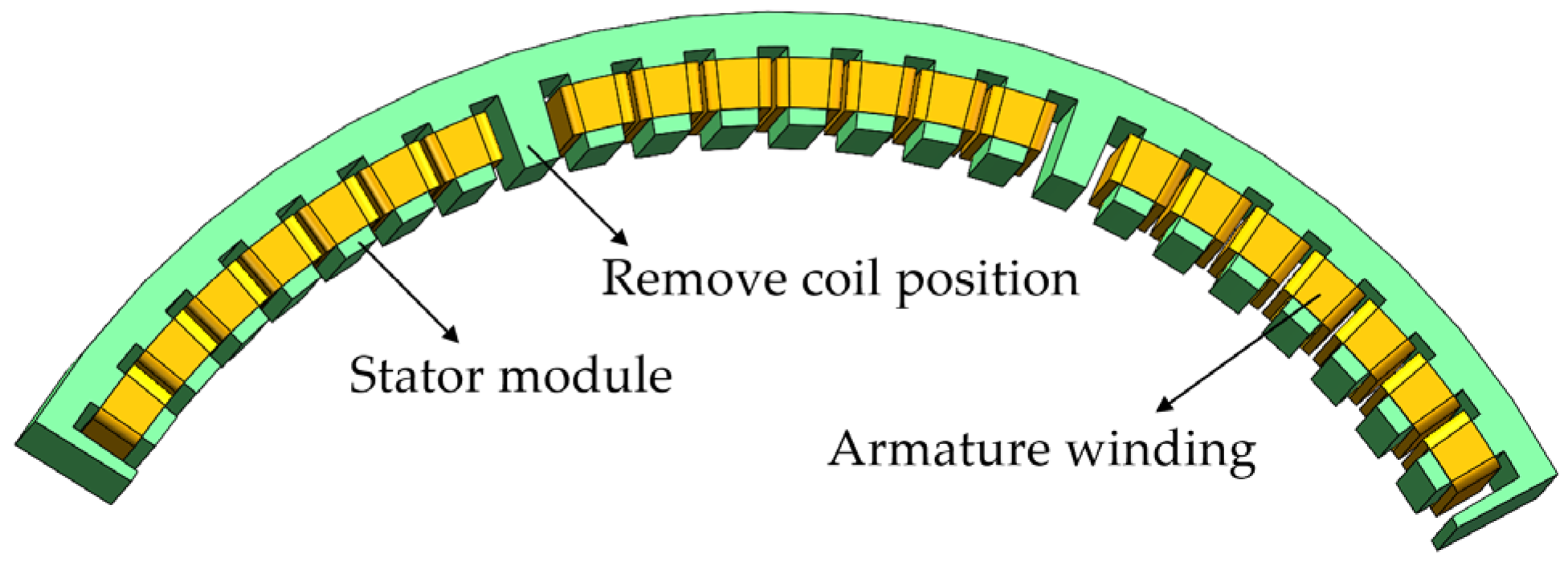
2.1. Electromagnetic Design of MFT-PMSMs

Under the premise of winding symmetry and magnetomotive force symmetry, the number of module combinations of the motor can be the greatest common divisor of the number of poles and slots. If the motor has a total of K coils, after removing N coils in the radial direction, it only needs to increase the axial length to the original K/(K − N) to achieve the overall electromagnetic performance unchanged [19]. This paper removes three coils from each of the three phases of the motor and divides it into three modules in the radial direction. The modules can be powered independently or in parallel by a controller. The winding uses rectangular copper wire with a parallel slot to achieve high wire slot fill. The single stator module and corresponding winding arrangement are shown in Figure 1.

In order to facilitate processing and improve torque performance, the rotor structure uses tangential permanent magnets. The permanent magnet is designed in segments along the axial direction to reduce the risk of damage during assembly. The cooling system is designed as an axial water-cooling system. The three-dimensional model of MFT-PMSMs is shown in Figure 2, and the rated parameters are shown in

Table 1. Main parameters of MFT-PMSM.

Parameter	Value	Unit
Outer diameter	1400	mm
Inner diameter	1225	mm
Axial length (Before/After module)	590/665	mm
Slots/Poles	72/60
PM thickness	14	mm
Air-gap length	2	mm
Iron core type	50WW470
PM materials	N38SH
Operational speed	75	r/min
Maximal torque	59,000	Nm
DC Bus Voltage	8000	V

.

According to the operating conditions, MFT-PMSM can be divided into rated load operation, short-term overload operation, and fault-tolerant operation. The input current and output torque under various operating conditions are shown in

Table 2. Electromagnetic torque under various operating conditions.

Operating Conditions	Current (A)	Electromagnetic Torque (kN/m)
Rated load condition	86	55.2
Overload condition	129	78.6
Single module fault condition	86	36.8

.

For the MFT-PMSM in this paper, it can output a rated torque of 55.2 kN/m when a rated current of 86 A is applied. Applying 1.5 times the rated current during overload operation can output 1.43 times the rated torque of 78.6 kN/m. When the motor winding fails, the fault module is cut off, and the remaining modules input the rated current to enable the overall motor to operate at reduced power. It can also input a larger overload current to make the non-fault module work in the overload state and output the rated power. However, under the same cooling conditions, the increase of current will lead to the increase of winding temperature, and the motor can only run for a short time in this state. Therefore, the accurate design of input current and running time during fault-tolerant operation is an important prerequisite to ensure the safety and life of the motor.

2.2. Loss Calculation of MFT-PMSM

The loss of the motor during operation mainly includes copper loss P_cu generated by the winding, iron loss P_fe generated by the stator core, eddy current loss P_pm of the permanent magnet, mechanical loss P_f, and stray loss P_s. The loss leads to the increase of the temperature of each part of the motor, especially for the windings and permanent magnets. Once the temperature exceeds the limit, the loss of the motor will occur. Therefore, it is of great significance to reasonably select the heat capacity of MFT-PMSM and accurately calculate the loss and temperature rise of the motor to improve the operation reliability of the motor.

The copper loss P_cu can be calculated as:

P_cu = I_rms²·R_cu

(1)

where I_rms is the stator winding current with rms value; R_cu is the resistance in windings.

The stator iron loss P_fe can be calculated by Bertotti’s model as:

P_fe = P_h + P_e + P_a = K_h f B_mⁿ + K_e f² B_m² + K_a f^1.5 B_m^1.5

(2)

where P_h, P_e, and P_a are hysteresis loss, eddy current loss, and additional loss, respectively. K_h, K_e, and K_a are hysteresis loss coefficient, eddy current loss coefficient, and additional loss coefficient, respectively. f and B_m are the alternating frequency and magnitude of the magnetic flux density, respectively.

The PM eddy current loss P_pm can be calculated as:

P_PM = ρ_PM·J²_PM·V_PM

(3)

where ρ_PM is the PM resistivity; J_PM is the eddy current density in the PM; V_PM is the volume of the PMs.

The mechanical loss P_f, while in the low-speed water-cooled motor of this paper, includes bearing loss and wind friction loss, which can be ignored. For each working condition in Table 2, this paper uses the FEM to obtain the losses, as shown in

Table 3. Loss of SSPMM under different operating conditions.

Operating Conditions	Loss Category	Value
Rated load condition	copper loss Pcu	14,377.9
	stator iron loss Pfe	11,943.6
	PM eddy current loss Ppm	630.9
Overload condition	copper loss Pcu	31,997.8
	stator iron loss Pfe	13,492.2
	PM eddy current loss Ppm	1227.6
Single module fault condition	copper loss Pcu	9585.3
	stator iron loss Pfe	7961.5
	PM eddy current loss Ppm	450.8

The loss units in the table are all in watts. Iron loss and eddy current loss exist in the whole core and magnetic steel, and copper loss only exists in the operation module.

.

3. Thermal Network Algorithm Considering Temperature Change of Cooling Medium

The hot network method uses a centralized parameter model to replace the internal distributed parameters of the motor, and achieves modeling by discretizing the various components of the motor into active and passive nodes. These nodes are interconnected through thermal conductivity and convective heat transfer resistance, and their temperature distribution is obtained by solving the heat balance equation system. However, in conventional thermal network models, the discretization of windings and iron cores is too rough, which limits the computational accuracy of the model. At the same time, the temperature change of cooling medium such as cooling water is also ignored. In fact, due to the heat exchange effect, there may be a great difference between the inlet temperature and the outlet temperature, which makes it difficult for the traditional thermal network method to accurately reflect the temperature difference on the circumference.

In this paper, a high-precision thermal network method considering the temperature change of cooling medium is proposed. By multi-layer meshing and dividing the model into blocks on the circumference, the calculation accuracy is improved and the temperature rise of the cooling medium is considered.

Specifically, on the axial cross-section of PMSM, heat transfer and temperature gradients at different axial positions can be reflected by dividing the winding into multiple layers. On the radial cross-section, PMSM can be divided into sectors according to the cooling structure, taking into account the influence of the temperature rise of the cooling medium on the heat dissipation capacity and final temperature of PMSM.

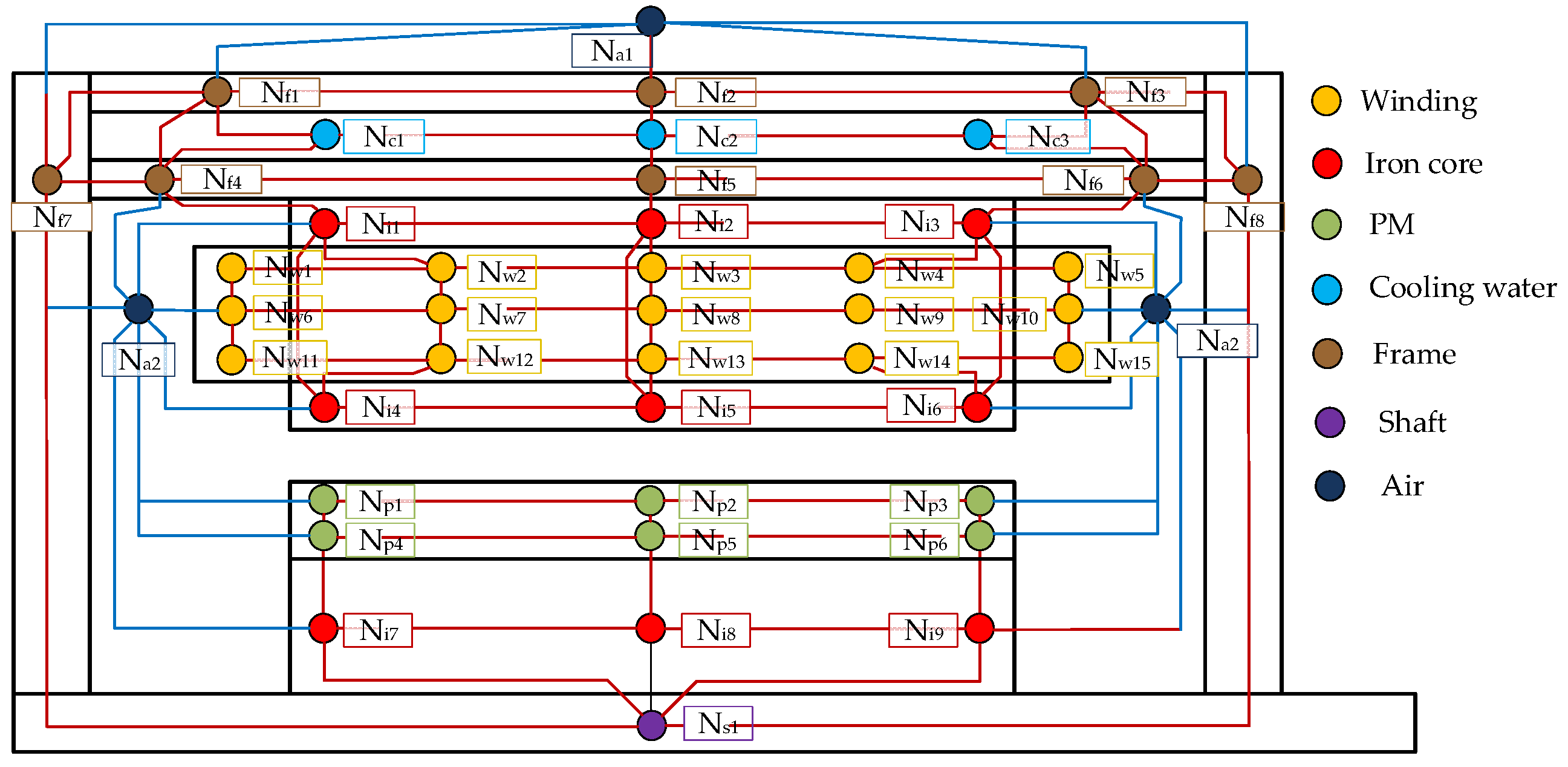
3.1. Construction of Thermal Network Model

The multi-layer thermal network model of MFT-PMSM is shown in Figure 3. In order to accurately reflect the temperature difference of windings at different positions, the windings, permanent magnets, and stator cores are divided into multiple layers. In Figure 3, N_a* represents the air node, N_w* represents the winding node, N_i* represents the stator and rotor core node, N_p* represents the permanent magnet node, N_s* represents the shaft node, N_f* represents the frame and end cover node, and N_c* represents the cooling medium node. In Figure 3, the red line indicates the thermal conduction path within the solid medium, while the blue line shows the convective heat transfer path in the air gap or cooling medium. Each path corresponds to a thermal resistance.

3.2. Thermal Network Parameters Calculation

3.2.1. Thermal Resistance Calculation

When the model is equivalent, it is necessary to set the assumptions first, which are:

(1) The ambient temperature remains invariant throughout the system operation and is not affected by the temperature change of the motor [6,7];

(2) The internal heating of each component of the motor is balanced, and there is no local heating;

(3) The cooling medium is completely in contact with the tube wall, and there is no imbalance of convective heat transfer;

(4) Temperature-induced variations in thermal conductivity and specific heat capacity of winding/core/PM materials are neglected.

When the thermal resistance is equivalently calculated by the motor model, the motor is divided into N parts along the circumference, and the loss of the active node in each part and the corresponding temperature rise of each part are calculated. In the first part, the temperature of the cooling medium is the initial temperature, and the temperature of the cooling medium in the second part is the temperature after considering the heat exchange in the first part. By analogy, the temperature of each part of the motor, considering the temperature rise of the cooling medium, can be obtained.

The convective thermal resistance and the conduction thermal resistance inside the motor can be calculated. The conduction thermal resistance is related to the heat transfer area A_{i_j}, the specific heat capacity λ_i, and the heat transfer path length L_i, which can be expressed as [20]:

R_{i_j} = L_i/(λ_i·A_{i_j})

(4)

The convective thermal resistance can be expressed as:

R_{i_j} = L_i/(λ_i·A_{i_j}) + 1/(α_i·S_{i_j})

(5)

where α_i is the convective heat dissipation coefficient; S_i is the convective heat dissipation area. The symbols and corresponding meanings for calculation are further defined in

Table 4. Symbol Definitions used in Thermal Network Computing.

Symbol	Physical Meaning	Corner Meaning
Ri_j	The thermal resistance	Unit i and unit j
Ai_j	Heat conduction area	Contact unit i and j
Li	Heat transfer axial length	unit i
Si_j	Thermal convection area	Contact unit i and j
λi	Thermal conductivity	Unit i
αi	Convective heat transfer coefficient	Unit i
hi	Heat transfer radial length	Unit i

.

Taking node N_i1 as an example, it has five heat exchange paths, which are heat conduction with winding node N_w2, stator node N_i2, stator node N_i4, casing node N_f4, and heat convection with air node N_a2. The thermal resistance between these nodes can be calculated as follows:

R_{i1_w2} = h_s/(2λ_s·A_{i1_w2}) + h_i/(2λ_i·A_{i1_w2})

(6)

A_{i1_w2} = (πb_s2/2 + 2h_t)·L_wi/3

(7)

where R_{i1_w2} denotes the thermal conduction resistance between node N_i1 and node N_w2; A_{i1_w2} represents the radial heat transfer area at the yoke insulation; h_i is the thickness of the winding insulation material; λ_i is the thermal conductivity of the winding isolation; b_s2 corresponds to the bottom radius of the stator slot; h_t is the tooth length; L_wi is the axial coverage length of the winding insulation.

R_{i1_a2} = (L_s/6)/(λ_ic·S_{8_1}) + 1/(α_r·S_{i1_a2})

(8)

S_{i1_a2} = π(D²₁ − D²_i1)/4 − Z_s·(h_t (b_s1 + b_s2)/2 + πb_s2²/4)

(9)

where R_{i1_a2} is the thermal conduction resistance between stator yoke node N_i1 and air-gap node N_a2; S_{i1_a2} is equivalent circumferential conduction area at the yoke-airgap interface; λ_ic is axial thermal conductivity of laminated core (parallel to stacking direction); D₁ and D_i1 are diameters of the stator core, respectively; Z_s is the slot number; b_s1 is the stator slot opening width; α_r is the convective coefficient on the stator end surface.

R_{i1_i2} = (L_s/3)/(λ_ic·A_{i1_i2})

(10)

A_{i1_i2} = A_{i1_w2}

(11)

where R_{i1_i2} is the axial conductive resistance between stator yoke node N_i1 and node N_i2; L_s is the axial length of stator core lamination stack.

R_{i1_i11} = L_slot/(λ_ic·A_{i1_i11})

(12)

A_{i1_i11} = L_s·A_slot

(13)

where R_{i1_i11} is the radial conductive resistance from yoke node N_i1 and node N_i11; L_slot is the length of the stator slot in radial direction; A_{i1_i11} is the tooth width; A_slot is effective heat transfer area at tooth tip.

R_{i1_f4} = h_f/(4λ_f·A_{i1_f4}) + h_s/(2λ_ic·A_{i1_f4}) + L_g/(λ_a·A_{i1_f4})

(14)

A_{i1_f4} = π D_s·L_s/3

(15)

where R_{i1_f4} is the interface thermal resistance between N_i1 and node N_f4; A _{i1_f4} is the contact area of the frame and stator yoke; h_s is the radial thickness of stator yoke back iron; L_g is the assembly clearance between the stator and the frame; λ_a is the thermal conductivity of air; D_s is the diameter of the stator.

For the cooling node N_c1, the heat transfer path includes three paths, namely, the heat convection between the cooling medium N_c1 and the frame N_f1 and N_f4, and the heat conduction between the cooling nodes N_c1 and N_c2. The thermal resistance between these nodes can be calculated as follows:

R_{c1_f1} = (h_f/4)/(λ_f·A_{c1_f1}) + 1/(α_f·S_{c1_f1})

(16)

A_{c1_f1} = π D_f·L/3

(17)

S_{c1_f1} = C·L/3

(18)

where R_{c1_f1} is the composite resistance between frame node N_c1 and node N_f1; h_f is the wall thickness of motor frame; λ_f is the thermal conductivity of the frame; A_{c1_f1} is radial conduction area at frame-coolant interface; S_{c1_f1} is the convective heat transfer area of coolant channel surface; α_f is the convective heat transfer coefficient of the cooling medium; D_f, L_f and C_c are the equivalent diameter, length and channel circumference of the casing respectively.

R_{c1_c2} = L/(3λ_f·A_{c1_c2})

(19)

where R_{c1_c2} is the circumferential conductive resistance between adjacent frame node N_c1 and node N_c2; A_{c1_c2} is the cross-sectional area along circumferential direction.

Between the nodes in Figure 3, both the convective thermal resistance and the conduction thermal resistance can be calculated by the method of each node. The complete thermal network model can be obtained by substituting it into Figure 3. The local thermal network is shown in Figure 4.

3.2.2. Calculation of Convective Heat Transfer Coefficient

The thermal resistance between the nodes in the motor includes conduction thermal resistance and convection thermal resistance. The convection thermal resistance can be solved based on the Reynolds number of the flow state.

Firstly, the flow rate of the cooling medium is calculated:

v = V/A_c

(20)

where v is the flow rate of the cooling medium; V is the flow of the cooling medium; A_c is the cooling pipe cross-sectional area.

The calculation formula of Reynolds number Re is:

Re = v·D_c/v_d

(21)

where D_c is the characteristic length, for pipe flow, is usually the pipe diameter (m); v_d is the dynamic viscosity of cooling medium.

According to the calculation results of Re, the flow state of the cooling medium can be judged. When Re < 2300, the cooling medium is in laminar flow state; when 2300 < Re < 4000, the cooling medium is in the transition flow state; when Re > 4000, the cooling medium is in turbulent state.

Further, the Prandtl number is determined according to the temperature of the cooling medium, and then the Nusselt number Nu is calculated. The calculation formula is [21]:

Nu = 0.023·Re^0.8·Pr^0.3

(22)

Nu = 1.86·(Re·Pr·D_c/L)^0.33

(23)

Nu = (f/8)(Re − 1000)·Pr/((1 + 12.7)·sqrt(f/8)(Pr^2/3 − 1))

(24)

Finally, the convective heat transfer coefficient α_c can be calculated as:

α_c = Nu·k/D_c

(25)

The circumferential convective heat transfer coefficient α_g can be expressed as [22]:

α_g = N_ug·λ_g/g

(26)

N_ug = 0.128(T_a²/F_g²)^0.367

(27)

T_a = r_a^0.5·g^1.5·n/v_a

(28)

where g is the radial air gap length; r_a is the effective air gap diameter; n is the rotational speed; v_a is the kinematic viscosity of air; F_g is a Geometrical correction factor (accounts for slot-pitch effects and end leakage).

The end face convective heat transfer coefficient α_r can be expressed as [22]:

α_r = 2N_ur·λ_a/D_i

(29)

N_ur = 1.67R_er^0.385

(30)

R_er = π·D_i²·n/120v_a

(31)

where D_i is the equivalent diameter of end face.

3.3. Calculate Temperature Using Transient Heat Conduction Equation

The transient heat conduction equation of heat exchange during motor operation is established in this paper to solve the transient temperature of the motor. The loss of each equivalent node and the corresponding thermal resistance are brought into the equation to solve the temperature change of the motor.

In order to speed up the calculation efficiency and improve the calculation accuracy, this paper uses the fourth-order Runge-Kutta method to solve the heat conduction equation of the motor. The slope of each point of the fourth-order Runge-Kutta method can be expressed as:

k₁ = f(t_n, T_n)

(32)

k₂ = f(t_n + Δt/2, T_n + Δt/2·k₁)

(33)

k₃ = f(t_n + Δt/2, T_n + Δt/2·k₂)

(34)

k₄ = f(t_n + Δt, T_n + Δt·k₃)

(35)

T_n+1 = T_n + Δt/6·(k₁ + k₂ + k₃ + k₄)

(36)

Set the initial temperature distribution and time step Δt of the motor during the simulation initialization phase. Based on the pre-calculated power distribution of the motor heat source, thermal conductivity, and convective thermal resistance parameters, the temperature field at time t + Δt is obtained by recursively solving the transient thermal equilibrium equation. The calculation process continues to iterate until the set simulation duration is reached.

3.4. Temperature Solution Results and Analysis

In this section, the calculation model proposed in this paper is used to check the temperature of the motor under different operating conditions. The system flow chart during the analysis is shown in Figure 5. The temperature verification of the motor can be regarded as a continuation of electromagnetic design. From Figure 5, it can be seen that in the design phase, the electromagnetic parameters of the motor are first designed, and then the motor is designed by module combination according to the method in Section 2.1. After meeting the required electromagnetic performance requirements, the losses are calculated and the temperature is calculated and verified using the thermal network algorithm proposed in this article. If the temperature is unreasonable, the electromagnetic design is re-carried out.

According to the winding characteristics of the motor in Figure 2, the thermal network of the motor can be divided into six parts along the radial direction, and the heat source of each part is 1/6 of the loss of the motor component. The inlet temperature of the second part is the outlet temperature of the first part, and so on.

According to the flow chart of Figure 5, the temperature of each part of the motor running in the rated state of the MFT-PMSM is calculated as shown in

Table 5. Calculated node temperature during rated operating conditions.

Components	Node/Temperature
Environment	Na1/303.15
Stator yoke		Ni1/328.7	Ni2/326.2	Ni3/328.7
Stator tooth		Ni4/349.9	Ni5/348.7	Ni6/349.9
Winding	Nw1/370.4	Nw2/368.1	Nw3/367.3	Nw4/368.1	Nw5/370.4
	Nw6/371.7	Nw7/368.5	Nw8/367.8	Nw9/368.5	Nw10/371.7
	Nw11/373.3	Nw12/370.5	Nw13/368.7	Nw14/370.5	Nw15/373.3
Permanent Magnet		Np1/362.5	Np2/369.4	Np3/362.5
		Np4/364.7	Np5/367.9	Np6/364.7
Rotor core		Ni7/360.1	Ni8/362.4	Ni9/360.1

The temperature units are all in Kelvins.

.

It can be seen from Table 5 that the temperature at the end of the motor winding is the highest, and the closer to the air gap, the higher the temperature. The temperature of the permanent magnet is relatively high due to poor heat dissipation conditions. Therefore, for MFT-PMSM, it is also very important to analyze the temperature of the permanent magnet. Further, the cooling water temperature, winding, and permanent magnet temperature of different parts can be obtained, which can be seem in

Table 6. Maximum temperature of cooling water, winding, and permanent magnet in different parts.

Components	Temperature
	Part 1	Part 2	Part 3	Part 4	Part 5	Part 6
Cooling water	305.4	306.5	307.7	309	310.3	311.5
Winding	373.3	374	374.5	374.9	375.6	376.3
Permanent Magnet	369.4	369.4	369.5	369.5	369.6	369.7

The temperature units are all in Kelvins.

.

From the results of different parts, it can be seen that the temperature of cooling water increases with the heat exchange, which leads to the increase of the maximum temperature of the corresponding part of the winding. The maximum temperature difference between the winding of the first part and the sixth part reaches 8 degrees. Since this paper does not consider the influence of different parts of the temperature on the loss, and there is basically no heat exchange between the stator and the rotor, the temperature of the permanent magnet of each part of the rotor is basically unchanged.

When the motor overload operation occurs, input is 1.5 times the rated current. Under this operating condition, the heat dissipation capacity of the motor is not enough to run continuously, so it is necessary to calculate the maximum allowable working time of the overload condition. After the calculation in this paper, when the MFT-PMSM runs under overload conditions for 12 min, the winding temperature is close to the temperature limit of F-level insulation. The temperature of each component of MFT-PMSM after operating under overload conditions for 12 min is shown in

Table 7. Calculated node temperature during overload operating conditions.

Components	Node/Temperature
Environment	Na1/303.3
Stator yoke		Ni1/378.5	Ni2/374.8	Ni3/378.5
Stator tooth		Ni4/394.7	Ni5/392.9	Ni6/394.7
Winding	Nw1/419.7	Nw2/415	Nw3/419.1	Nw4/415	Nw5/419.7
	Nw6/421.4	Nw7/418	Nw8/410.8	Nw9/418	Nw10/421.4
	Nw11/422.1	Nw12/418.4	Nw13/411.9	Nw14/418.4	Nw15/422.1
Permanent Magnet		Np1/383.3	Np2/386.4	Np3/383.3
		Np4/386.6	Np5/388.5	Np6/386.6
Rotor core		Ni7/374.1	Ni8/375.0	Ni9/374.1

The temperature units are all in Kelvins.

.

When one module of MFT-PMSM fails, the other two modules can work normally. At this time, the motor can input the rated working current to reduce the power operation, and can also input the overload current to output the rated power in a short time. As shown in Figure 2, the two modules of MFT-PMSM are not only electromagnetically isolated, but also physically isolated by isolation teeth. The temperature of each module is basically not affected by other modules. Therefore, the temperature rise of the motor in the fault-tolerant operation state is not much different from that in the rated state and overload state. This paper does not list the calculated temperature.

4. Fluid-Solid Coupling Temperature Simulation

In this paper, the fluid-solid coupling finite element method (FEM) is used to simulate the temperature of each part of MFT-PMSM under different working conditions. Before the simulation, some model equivalence and assumptions need to be made:

(1) The ambient temperature of the motor is set to 303.15 Kelvins, and the ambient temperature does not change with the operation of the motor.

(2) The inlet temperature of the cooling water is constant at 306.15 Kelvins, and it is always supplied by a special water pump during operation, and the water flow remains constant;

(3) It is considered that the components in the motor are in close contact, and the tiny gap of the welding fins of the cooling water channel is ignored;

(4) Ignore the variation of physical properties of motor components with temperature;

(5) The winding is equivalent to copper bar, and the slot insulation, interlayer insulation, and copper wire insulation are equivalent to the copper bar.

The properties of the materials of each part of the motor are shown in

Table 8. Material properties of components in MFT-PMSM.

Components	Material	Density (kg/m3)	Specific Heat Capacity (J/kg·K)	Thermal Conductivity (W/m·K)
Frame	20Mn2	7850	460	45
Stator	DW465	7650	460	30
Winding	Copper	8980	381	387.6
Permanent Magnet	NdFeB	7500	460	7.6
Rotor yoke	40Cr	7850	460	42.7

.

In this paper, the finite element software is used to analyze the MFT-PMSM to simulate the motor temperature under different working conditions. In order to ensure the calculation accuracy, the motor is meshed, and a high-performance workstation with 256 G memory is used for calculation. It is worth noting that the modeling and simulation of fluid-solid coupling takes about 15 h. The temperature of winding, permanent magnet, rotor core, and cooling water of MFT-PMSM obtained by simulation is shown in Figure 6.

From Figure 6, it can be seen that the highest temperature in the motor occurs at the end of the winding, and the heat at the end of the winding can only be conducted to the inside of the slot through the path of “cooling water for the stator core of the winding”. Meanwhile, the coil temperature at the module combination location is lower than that at the non-module combination location, because only a single-layer coil exists at the module combination location. In addition, although the permanent magnet loss in MFT-PMSM is low, the temperature is also high due to relying solely on air convection heat transfer, reaching a maximum temperature of 368.2 Kelvin. From Figure 6d, it can be seen that the temperature of the cooling water also changes with the progress of heat exchange, and the outlet water temperature increases significantly relative to the inlet water temperature, indicating that the heat exchange capacity at the outlet position will be weaker than that at the inlet position. According to the previous analysis, ignoring this phenomenon will lead to inaccurate temperature calculations.

The temperature of each part of the MFT-PMSM calculated by the fluid-solid coupling FEM and the temperature calculated by the temperature network model proposed in this paper are shown in

Table 9. Maximum temperature of each component under rated condition.

Components	Fluid-Solid Coupling Analysis	Network Method	Relative Error
Winding	371.7	376.3	1.23%
Permanent Magnet	368.2	369.7	0.41%
Cooling water	314.5	311.5	0.95%

The temperature units in the table are all in Kelvins.

. It can be seen that the method proposed in this paper has high precision and can accurately calculate the temperature of MFT-PMSM. Compared with the fluid-solid coupling finite element method, the method used in this paper does not need to establish a complex three-dimensional model, and has strong versatility. The total time of modeling and calculation only takes a few minutes.

Because the calculation of fluid-solid coupling FEM is very time-consuming, the transient temperature rise of MFT-PMSM under overload condition is not calculated in this paper. The temperature rise of the single module fault calculated by this method when the double module still inputs the rated current is shown in Figure 7.

Because the calculation of fluid-solid coupling FEM is very time-consuming, the transient temperature rise of MFT-PMSM under overload condition is not calculated in this paper. For the MFT-PMSM studied in this paper, a single-step fluid structure coupling simulation takes about 15 h. When calculating overload conditions, it is necessary to calculate the temperature change of the motor at fixed time intervals, which often requires dozens or even tens of steps of fluid structure coupling simulation. Although fluid structure coupling simulation is generally considered more accurate, its extremely time-consuming nature often makes it difficult to utilize in practical applications. By comparison, the method proposed in this article is highly suitable for motor design and thermal design by motor design engineers.

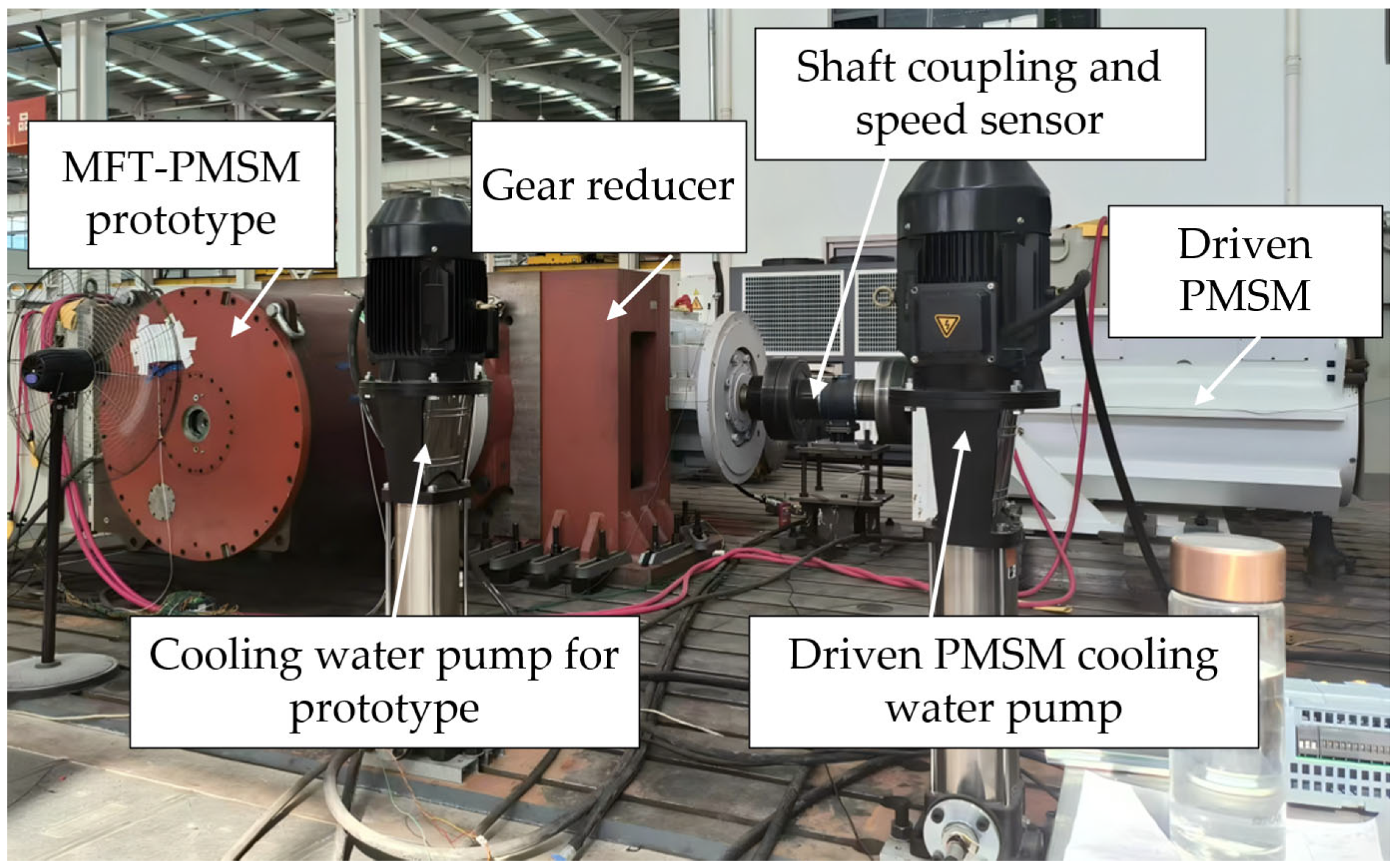
5. Experimental Verification

In order to accurately verify the accuracy of the proposed method, a load experimental platform of MFT-PMSM is built. The experimental platform mainly includes a 400 kW MFT-PMSM with a rated speed of 75 r/min, a driven motor used as a prototype load, two water pumps for motor cooling water supply, gear reducer and coupling, sensors, etc. The temperature test platform is shown in Figure 8. The speed and torque sensor adopts HCNJ-101 from Haibohua Company, Shenzhen, China, and the data is transmitted to the upper computer through a dual data conversion module. The temperature sensor is PT1000, and the winding temperature at the corresponding position can be obtained by measuring the change in resistance. Due to the inability to capture the location of the temperature sensor during the offline assembly of the motor, the placement of the temperature sensor in this article is listed in

Table 10. The position of the temperature sensor and the detected temperature.

Temperature Sensor	Position	Detected Temperature
S1	Winding end, close to outlet	381.15 K
S2	Winding ends, on the radial circumference	376.25 K
S3	Winding ends, on the radial circumference	374.45 K
S4	Winding end, close to inlet	373.55 K
S5	Middle of the winding, located in stator slot	367.75 K

.

The temperature sensor PT1000 from Haibohua Company, Shenzhen, China used in this article has been calibrated according to IEC60751 before the experiment [23]. The resistance of the temperature sensor at the reference temperature of 273.15 Kelvins is 1000 ohms. The resistance within the experimental measurement range can be expressed as follows:

R(t) = R₀·(1 + A·t + B·t²)

(37)

where A and B are temperature coefficients. A is equal to 3.9083 × 10⁻³, B is equal to −5.775 × 10⁻⁷. It can be seen that measuring the real-time temperature of PT1000 can calculate the resistance value at the corresponding measurement location.

When the motor is manufactured, five temperature sensors are embedded in the winding slot and at the end to detect the temperature of the motor during operation. One of the temperature sensors is placed in the middle of the slot, two temperature sensors are set near the inlet and outlet, and the remaining two are distributed along the radial circumference. The temperature sensor can be defined as S₁ to S₅, respectively. The temperature of different sensors obtained by the experiment is shown in Figure 9.

The tested MFT-PMSM runs at rated power, and the temperature is basically stable after 400 min of testing. The position of the five temperature sensors and the detected temperature are shown in Table 10.

It can be seen from the results that the maximum temperature of the winding measured by the experiment is 381.15 K. The calculation result of the method proposed in this paper is 376.3 K, and the absolute error is 1.27%. The MFT-PMSM temperature network algorithm proposed in this paper can accurately calculate the motor temperature, and consider the influence of cooling water temperature change on the motor temperature rise.

6. Conclusions

Aiming at the problem of low thermal analysis efficiency and limited accuracy of MFT-PMSM, an efficient and high-precision thermal network algorithm is proposed in this study. This method divides the physical structure of the equivalent motor by hierarchical nodes, and combines the fourth-order Runge-Kutta method to significantly improve the calculation efficiency, and innovatively considers the influence of the temperature rise of the cooling medium on the spatial temperature distribution. Based on the finite element method, the multi-condition loss distribution is obtained and mapped to the thermal network node, and the rapid calculation of the temperature rise of key components such as windings and permanent magnets is realized. Fluid simulation and prototype experimental verification show that the calculation error of key temperature under rated conditions is less than 1.2%, the overload condition accurately predicts the safe operation time limit of 12 min, and the calculation efficiency is significantly improved compared with the traditional CFD method. This method provides an efficient and reliable tool for motor design, especially for thermal safety assessment and optimization under extreme conditions and failure modes.

References

1. Jiang, X.; Zhang, Z.; Ma, K.; Weng, X.; Bu, F. Design and Analysis of a Fault-Tolerant Permanent Magnet Steering Motor for Electric Vehicles. IEEE Trans. Energy Convers. 2025, 40, 970–983. [Google Scholar] [CrossRef]
2. Tang, Y.; Chai, F.; Xie, Y.; Cai, W.; Guo, Q.; Tian, J. Investigation of Fault-Tolerant Performance and Inductance in a Modular Permanent Magnet In-Wheel Motor. IEEE Trans. Magn. 2023, 59, 1–6. [Google Scholar]
3. Zhang, B.; Gan, B.; Li, Q. Analysis of a Fault-Tolerant Module-Combined Stator Permanent Magnet Synchronous Machine. IEEE Access 2020, 8, 70438–70452. [Google Scholar] [CrossRef]
4. Zhang, L.; Deng, S.; Zhu, X.; Shen, D.; Chen, C.; Li, X. Multiple Operation Design and Optimization of a Five-Phase Interior Permanent Magnet Motor Considering Compound Fault Tolerance from Perspective of Flux-Intensifying Effect. IEEE Trans. Transp. Electrif. 2024, 10, 9043–9054. [Google Scholar] [CrossRef]
5. Madhavan, S.; P B, R.D.; Gundabattini, E.; Mystkowski, A. Thermal Analysis and Heat Management Strategies for an Induction Motor, a Review. Energies 2022, 15, 8127. [Google Scholar] [CrossRef]
6. Tang, Y.; Chen, L.; Chai, F.; Chen, T. Thermal Modeling and Analysis of Active and End Windings of Enclosed Permanent-Magnet Synchronous In-Wheel Motor Based on Multi-Block Method. IEEE Trans. Energy Convers. 2020, 35, 85–94. [Google Scholar] [CrossRef]
7. Bourgault, A.; Taqavi, O.; Li, Z.; Byczynski, G.; Kar, N.C. Advanced Lumped Parameter Thermal Network for Modeling of Cooling Solutions in Electric Vehicle Motor Applications. IEEE Trans. Magn. 2024, 60, 8205405. [Google Scholar] [CrossRef]
8. Ma, Y.; Xiao, Y.; Wang, J.; Zhou, L. Multicriteria Optimal Latin Hypercube Design-Based Surrogate-Assisted Design Optimization for a Permanent-Magnet Vernier Machine. IEEE Trans. Magn. 2022, 58, 1–5. [Google Scholar] [CrossRef]
9. Fasquelle, A.; Laloy, D. Water Cold Plates Cooling in a Permanent Magnet Synchronous Motor. IEEE Trans. Ind. Appl. 2017, 53, 4406–4413. [Google Scholar] [CrossRef]
10. Li, B.; Yan, L.; Cao, W. An Improved LPTN Method for Determining the Maximum Winding Temperature of a U-Core Motor. Energies 2020, 13, 1566. [Google Scholar] [CrossRef]
11. Wang, G.; Wang, Y.; Gao, Y.; Hua, W.; Ni, Q.; Zhang, H. Thermal Model Approach to the YASA Machine for In-Wheel Traction Applications. Energies 2022, 15, 5431. [Google Scholar] [CrossRef]
12. Li, C.; Zhang, H.; Hua, W.; Yin, H.; Zhang, K.; Su, L. Thermal Modeling and Loss Analysis of Fractional-Slot Concentrated Winding Permanent Magnet Motors for Improved Performance. IEEE Trans. Transp. Electrif. 2024, 10, 7151–7159. [Google Scholar] [CrossRef]
13. Yu, S.; Zhou, Y.; Wang, Y.; Zhang, J.; Dong, Q.; Tian, J.; Chen, J.; Leng, F. Optimization Study of Cooling Channel for the Oil Cooling Air Gap Armature in a High-Temperature Superconducting Motor. Electronics 2024, 13, 97. [Google Scholar] [CrossRef]
14. Hu, K.; Zhang, G.; Zhang, W. Rotor Design and Optimization of High-Speed Surface-Mounted Permanent Magnet Motor Based on the Multi-Physical Field Coupling Method. IEEE Access 2023, 11, 69614–69625. [Google Scholar] [CrossRef]
15. Ai, Q.; Wei, H.; Dou, H.; Zhao, W.; Zhang, Y. Robust Rotor Temperature Estimation of Permanent Magnet Motors for Electric Vehicles. IEEE Trans. Veh. Technol. 2023, 72, 8579–8591. [Google Scholar] [CrossRef]
16. Jing, H.; Chen, Z.; Wang, X.; Wang, X.; Ge, L.; Fang, G.; Xiao, D. Gradient Boosting Decision Tree for Rotor Temperature Estimation in Permanent Magnet Synchronous Motors. IEEE Trans. Power Electron. 2023, 38, 10617–10622. [Google Scholar] [CrossRef]
17. Tang, P.; Zhao, Z.; Li, H. Short-Term Prediction Method of Transient Temperature Field Variation for PMSM in Electric Drive Gearbox Using Spatial-Temporal Relational Graph Convolutional Thermal Neural Network. IEEE Trans. Ind. Electron. 2024, 71, 7839–7852. [Google Scholar] [CrossRef]
18. Jin, L.; Mao, Y.; Wang, X.; Lu, L.; Wang, Z. A Model-Based and Data-Driven Integrated Temperature Estimation Method for PMSM. IEEE Trans. Power Electron. 2024, 39, 8553–8561. [Google Scholar] [CrossRef]
19. Xu, Y.; Zhang, B.; Feng, G. Analysis of Unwinding Stator Module Combined Permanent Magnet Synchronous Machine. IEEE Access 2020, 8, 191901–191909. [Google Scholar] [CrossRef]
20. Xu, Y.; Zhang, B.; Feng, G. Research on Thermal Capacity of a High-Torque-Density Direct Drive Permanent Magnet Synchronous Machine Based on a Temperature Cycling Module. IEEE Access 2020, 8, 155721–155731. [Google Scholar] [CrossRef]
21. Welty, J.; Rorrer, G.L.; Foster, D.G. Fundamentals of Momentum, Heat and Mass Transfer, 6th ed.; John Wiley & Sons, Inc.: Hoboken, NJ, USA, 2014. [Google Scholar]
22. Lu, Q.; Zhang, X.; Chen, Y.; Huang, X.; Ye, Y.; Zhu, Z.Q. Modeling and Investigation of Thermal Characteristics of a Water-Cooled Permanent-Magnet Linear Motor. IEEE Trans. Ind. Appl. 2015, 51, 2086–2096. [Google Scholar] [CrossRef]
23. IEC60751; Industrial Platinum Resistance Thermometers and Platinum Temperature Sensors. International Electrotechnical Commission: Geneva, Switzerland, 2022.
Figure 1. Single module winding structure of MFT-PMSM.
Energies 18 03967 g001
Figure 2. The motor structure of MFT-PMSM.
Energies 18 03967 g002
Figure 3. The thermal network structure of MFT-PMSM.
Energies 18 03967 g003
Figure 4. Local detailed thermal network of MFT-PMSM.
Energies 18 03967 g004
Figure 5. MFT-PMSM temperature calculation flowchart.
Energies 18 03967 g005
Figure 6. Temperature distributions in MFT-PMSM under rated condition: (a) stator winding; (b) permanent magnet; (c) rotor core; and (d) cooling water.
Energies 18 03967 g006
Figure 7. Temperature distributions in MFT-PMSM under rated condition: (a) stator core; (b) stator winding.
Energies 18 03967 g007
Figure 8. MFT-PMSM temperature test experimental platform.
Energies 18 03967 g008
Figure 9. Test temperature curves under rated condition.
Energies 18 03967 g009