Dynamic Performance Design and Validation in Large, IBR-Heavy Synthetic Grids

Abstract

Cross-validation and open research on future electric grids, particularly in their stability modeling and dynamic performance, can greatly benefit from high-fidelity, publicly available test cases, since access to dynamic response models of actual grid models is often limited due to legitimate security concerns. This paper presents a methodology for designing and validating the dynamic performance of large, IBR-heavy synthetic grids, that is, realistic but fictitious test cases. The methodology offers a comprehensive framework for creating dynamic models for both synchronous generators (SGs) and inverter-based resources (IBRs), focusing on realism, controllability, and flexibility. For realistic dynamic performance, the parameters in each dynamic model are sampled based on statistical data from benchmark actual grids, considering power system dynamics such as frequency and voltage control, as well as oscillation response. The paper introduces system-wide governor design, which improves the controllability of parameters in dynamic models, resulting in a more realistic frequency response. As an example, multiple case studies on a 2000-bus Texas synthetic grid are shown; these represent realistic dynamic performance under different transmission conditions in terms of frequency, voltage control, and oscillation response.

1. Introduction

Modern power grids are undergoing a rapid transition to reduce carbon emissions and introduce innovative technologies. For instance, the Australian Energy Market Operator (AEMO) released the Engineering Roadmap to 100% Renewables, predicting that Australia’s National Electricity Market will be capable of meeting 100% of demand with renewable energy [1]. In the United States, the Electric Reliability Council of Texas (ERCOT) plans to add more than 30 GW of solar capacity within the next five years, effectively doubling its current solar capacity of approximately 30 GW [2]. The transformation of power grids presents a number of challenges, including the interconnection of high penetration of inverter-based resources (IBRs) [3,4,5,6]. Compared to traditional synchronous generators (SGs), IBRs do not inherently provide a frequency response through mechanical inertia because the mechanical physics in IBRs are decoupled from the electrical grid [7]. In order to enable IBRs to participate in frequency response, Grid Forming Inverter (GFM) technologies have been developed [8,9,10,11,12]. GFM also poses challenges, however, that need to be carefully developed and managed [13,14].

The challenges in power system transformation make power system planning crucial. Power system planning can identify anticipated issues and their solutions during the grid transition. To achieve this, transmission network models and their dynamic models are required to validate grid performance and system stability. However, accessing the actual grid model is difficult due to Critical Energy/Electric Infrastructure Information (CEII) restrictions. Synthetic grids offer an invaluable opportunity to researchers and engineers through open datasets that can be used for grid planning. Synthetic grids are fictitious power system models that statistically resemble actual grids but do not contain non-public data, allowing for realistic power system analyses through various public test cases without the limitations associated with accessing real-world data. Using synthetic grids enables research on future grids and cross-validation of the research for better grid planning.

Over the past few years, several studies have focused on developing synthetic grids for various purposes. Automated algorithms have been introduced to design realistic synthetic transmission networks that consider the geographical topology of electric power grids for modeling large-scale synthetic power grids [15]. From these well-designed synthetic transmission networks, research has extended toward designing generator dynamic models for synthetic grids. For example, studies have been conducted to design dynamic models and their parameters for SGs based on control system theory and statistics derived from actual systems [16,17]. In order to study the details in SGs’ dynamic models, a method for determining the parameters of exciters and governors has also been proposed [18]. Additionally, dynamic models for synthetic grids have been extended to include IBR dynamics for wind and solar, derived from statistical data from actual grids in [19]. Moreover, test models have been developed to study stability and security problems in AC-DC hybrid systems with high penetration of IBRs [20].

This paper introduces a comprehensive methodology to design and validate the dynamic performance of large, IBR-heavy synthetic grids. The methodology provides a framework to create validated dynamic models for both SGs and IBRs in positive sequence simulation, focusing on realism, controllability, and flexibility. To achieve realistic dynamic performance, parameters in each dynamic model are sampled based on statistical data from benchmark actual grids and validated according to power system dynamics. For governor parameter validation, frequency response is considered depending on the fuel type of units, and exciter and IBR parameters are validated based on voltage control response. For realistic stabilizer parameters, the oscillation response is analyzed. After determining the parameters in the dynamic models, each generator is validated from a small-signal stability perspective using eigenvalue analysis, and the interconnected system is validated through time-domain transient simulation. This paper applies a concept of system-wide governor design to enhance the controllability of frequency response. The system-wide governor is a low-order model that represents an aggregation of the system’s overall response. Faster transient simulations with this low-order model allow for parameter adjustments to achieve a more realistic system frequency response. The entire processes for synthetic grids with dynamic models are integrated into an automatic process, which helps to increase flexibility in generating dynamic models across various transmission networks. The algorithms are applied to the 2000-bus synthetic case on the footprint of Texas. Under different conditions including high/low-load and high/low-inertia scenarios, five test cases are validated in the perspectives of power system stability. Simulation results are displayed to validate the dynamic performance of the large and IBR-heavy synthetic grids which are generated by the proposed algorithm.

This paper is structured as follows: Section 2 describes the test cases used in this paper, and the detail methods are introduced in Section 3. In Section 4, the result of case study is described. Finally, Section 5 summarizes and concludes this paper.

2. Overview of 2000-Bus Synthetic Cases

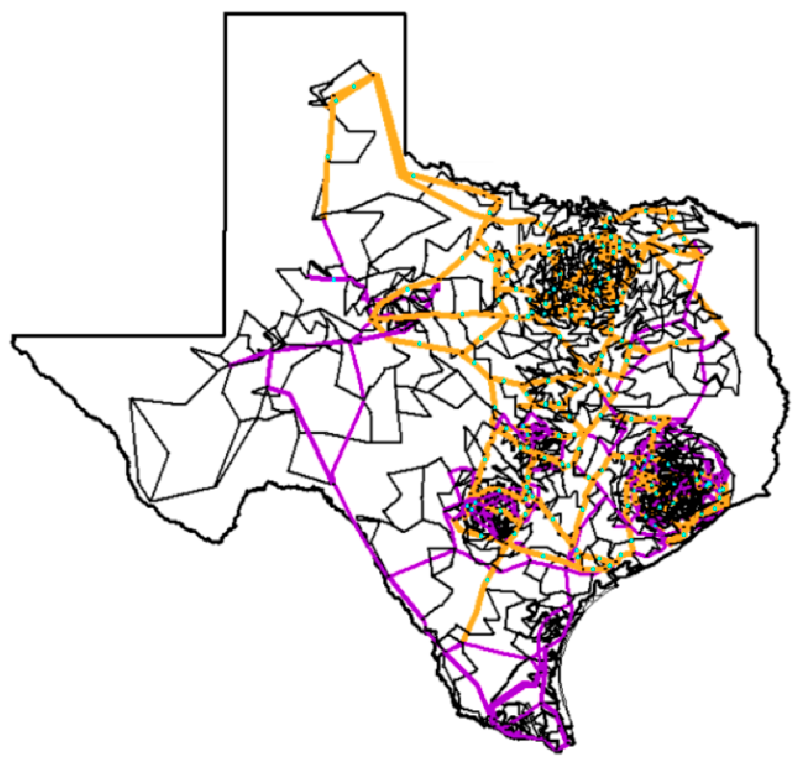
Before presenting the details of proposed method, it is helpful to introduce the test cases so that it can be referred to throughout the paper. For designing dynamic performance of synthetic grids, the Texas synthetic grid is used. This case is based on a 2000-bus synthetic grid shown in Figure 1 [21], with a transmission network that is geo-located in Texas but is fictitious, and it does not correspond to any actual grid. The summary of case information is provided in

Table 1. The summary of the base case.

Buses	Load [MW]	Generation (SGs) [MW]	Generation (IBRs) [MW]	Capacity (IBRs) [MW]
2000	$\mathrm{67,109}$	$\mathrm{57,886}$	$9223$	$\mathrm{13,168}$

.

Compared to the base case of the Texas synthetic grid created in 2016, recent actual Texas power grids have seen significant changes, particularly with a substantial increase in IBR capacity. According to an industry report [2], the current capacity of wind turbines in Texas is 39 GW, and the solar capacity is 23.5 GW. This report also provides the locations of the IBRs along with their respective capacities. Based on this information, the recent Texas synthetic transmission network is designed to reflect the realistic capacities and locations of the IBRs.

Five test cases have been developed using the methodology proposed in this paper to represent both past and recent Texas generation and load profiles on synthetic transmission networks.

Table 2. The summary of cases.

Case	Base	LL16	HL24	LL24	HRLL24
Wind capacity [GW]	12.4		39.5
Solar capacity [GW]	0.8		23.6
Wind generation [GW]	8.8		21.0		17.0
Solar generation [GW]	0.4		10.7		7.2
Total generation [GW]	68.7	37.7	91.0	52.1	34.3
Total load [GW]	67.1	36.9	87.6	49.7	32.4
%IBR penetration	13%	24%	35%	61%	71%

Base: High-load scenario in the 2016 Texas synthetic grids. LL16: Low-load scenario in the 2016 Texas synthetic grids. HL24: High-load scenario in the 2024 Texas synthetic grids. LL24: Low-load scenario in the 2024 Texas synthetic grids. HRLL24: High penetration of renewables and low-load scenario in the 2024 Texas synthetic grids.

provides detailed information about these cases. Beginning with the base case, a lower load and lower inertia scenario, referred to as LL16, is developed by reducing the load level and decommitting generators in the base case. These cases reflect the Texas power grids from the past 10 years. To represent high-load scenario in recent Texas grids (HL24), IBRs are added to the base case according to the report [2]. For LL24 case, which features lower load and lower inertia in recent network condition, loads are reduced, and generators are decommitted, following the same approach as in LL16 case. Additionally, HRLL24 case represents the highest penetration percentage of IBRs recorded in Texas and low-load scenario. In this case, the load and IBR generation are modified from HL24 scenario. These various versions of the Texas synthetic grid cases are publicly available in [21].

Table 2 also shows potential limitation of existing methods for building synthetic grids’ dynamics. Base and LL16 cases exhibit relatively low IBR penetration compared to HL24 through HRLL24 cases. Therefore, applying the methods proposed in [17,19] is relatively straightforward and does not introduce significant challenges in dynamic performance. However, manual tuning of individual generator parameters would be still necessary to achieve reasonably stable system behavior. In contrast, applying the same methodologies to HL24 through HRLL24 cases becomes increasingly difficult. This is primarily because previous approaches lack an explicit validation process for IBR stability and rely instead on statistical methods and system-level performance assessments. In scenarios with high IBR penetration, overall system stability tends to degrade, and these earlier approaches would demonstrate clear limitations in achieving a reasonably stable dynamic response. Therefore, this paper proposes a method designed specifically to ensure stability and realism in IBR-heavy scenarios.

Figure 2 presents the average bus frequency responses for the test cases under an N-2 contingency scenario involving the outage of the largest generators, using dynamic models developed with the proposed method.

Table 3. The summary of frequency response characteristics in each case.

Case	Base	LL16	HL24	LL24	HRLL24
Inertia [GW$·$s]	306.5	128.9	306.5	130.5	129.7
RoCoF [Hz/s]	0.46	1.06	0.42	0.87	1.25
Nadir [Hz]	59.71	59.29	59.70	59.36	59.36
Nadir time [Sec]	7.28	7.65	7.75	7.60	6.10

RoCoF: Rate of change of the frequency.

summarizes the frequency response characteristics. When IBRs are modeled as negative loads, the differences in frequency behavior among LL16, LL24, and HRLL24 cases are often not clearly captured, particularly when system inertia remains similar and low while IBR penetration levels vary. Furthermore, applying the method from [17,19] to systems with high IBR penetration does not guarantee stability and typically requires significantly more effort to achieve acceptable dynamic performance.

3. Methodology to Design and Validate Dynamic Models in Large and IBR-Heavy Synthetic Grids

The dynamic performance design in this paper aims to achieve a realistic and reasonably stable system response compared to benchmark actual systems. While statistical approaches are commonly used in dynamic performance design [16,17,18,19], the limited availability of benchmark system data can lead to overfitting issues. For example, some parameters in dynamic models have minimal impact on the dominant system response or exhibit poorly defined statistical distinctness, whereas others have a strong influence.

To address this challenge, this paper identifies and targets key parameters that significantly affect frequency, voltage, and oscillatory behavior. These critical parameters (${\mathit{\theta }}_{\mathit{c}}$) are sampled based on their relative probability distributions obtained from benchmark systems:

$${\theta }_i~p_i\left({\theta }_i\right),{\theta }_i\in {\mathit{\theta }}_{\mathit{c}}$$

where $p_i\left({\theta }_i\right)$ is the empirical probability density function of parameter ${\theta }_i$ based on benchmark data. The detailed critical parameter selection process is described in Section 3.1, Section 3.2 and Section 3.3.

The remaining non-critical parameters (${\mathit{\theta }}_{\mathit{n}\mathit{c}}$) are sampled using uniform distributions within parameter-specific bounds determined by the observed minimum and maximum values in benchmark grids:

$${\theta }_j~U({\theta }_j^{min},{\theta }_j^{max}),{\theta }_j\in {\mathit{\theta }}_{\mathit{n}\mathit{c}}$$

where $U({\theta }_j^{min},{\theta }_j^{max})$ is the uniform distribution between the minimum value ${\theta }_j^{min}$ and maximum value ${\theta }_j^{max}$ of parameter ${\theta }_j$ observed in the benchmark data.

Moreover, relying solely on system-level performance validation, as in prior studies, is inadequate for identifying the root causes of instability and limits effective diagnosis and correction. To overcome this limitation, this paper proposes a structured and modular validation framework encompassing three levels: individual model, individual generator with models, and overall system performance with generators. The validation metrics used in this framework are provided as suggested examples; they can be modified or expanded based on the specific requirements of systems under consideration. This layered approach enables the design of a reasonably stable dynamic response at each level:

• Individual model validation: The requirements for stable control systems, such as exciters and governors, are described in [22] and summarized in

  Table 4. The requirements for a stable control system.

  Gain Margin	Phase Margin	Damping Ratio
  Larger than 6 dB	Larger than 40°	Larger than 0.6

  . Key metrics, including phase margin, gain margin, and damping ratio, are calculated using open-loop and closed-loop analyses for each exciter and governor model, following standard practices [18].

• Individual generator validation: For each generator, eigenvalues are analyzed in a Single-Machine Infinite Bus (SMIB) system to ensure that no positive real eigenvalues exist. Additionally, IBRs must maintain adequate damping:

$$\underset{i\in \mathit{IBRs}}{\mathrm{m}\mathit{in}}{\zeta }_{min,i}<\epsilon$$

where ${\zeta }_{min,i}$ is the minimum damping ratio of generator $i$, and $\epsilon$ is threshold for acceptable damping ratio. In this paper, $\epsilon =0.6$ is used.

• Overall system performance validation (Multi-machine): The dynamic response of the entire interconnected system is validated using transient stability simulations. System stability is evaluated based on rotor angle deviation:

$$\underset{i\in \mathit{Generators}}{\max }\left|{\delta }_{max,i}-{\delta }_{initial,i}\right|<\epsilon$$

where ${\delta }_{max,i}$ is the maximum rotor angle of generator $i$, ${\delta }_{initial,i}$ is the initial rotor angle of generator $i$, and $\epsilon$ is threshold for acceptable rotor angle deviation. In this paper, $\epsilon =90°$ is used.

The validation process includes both small-signal and transient stability analyses using established analytical methods and simulation tools. Small-signal stability is evaluated through eigenvalue analysis of linearized dynamic models. As an initial step, SMIB system is used to verify eigenvalue locations and assess local oscillatory modes. This approach can be extended to multi-machine systems to capture inter-area oscillations relevant to large-scale interconnected grids. Transient stability is assessed via time-domain simulations using the PowerWorld Simulator to evaluate rotor angle response under disturbance scenarios. While this study primarily uses damping ratio and rotor angle deviation as the key stability metrics, the proposed framework also supports the use of additional indicators such as frequency nadir, voltage deviation, and critical clearing time. These additional metrics are employed in this paper to comprehensively evaluate the dynamic models generated by the proposed method.

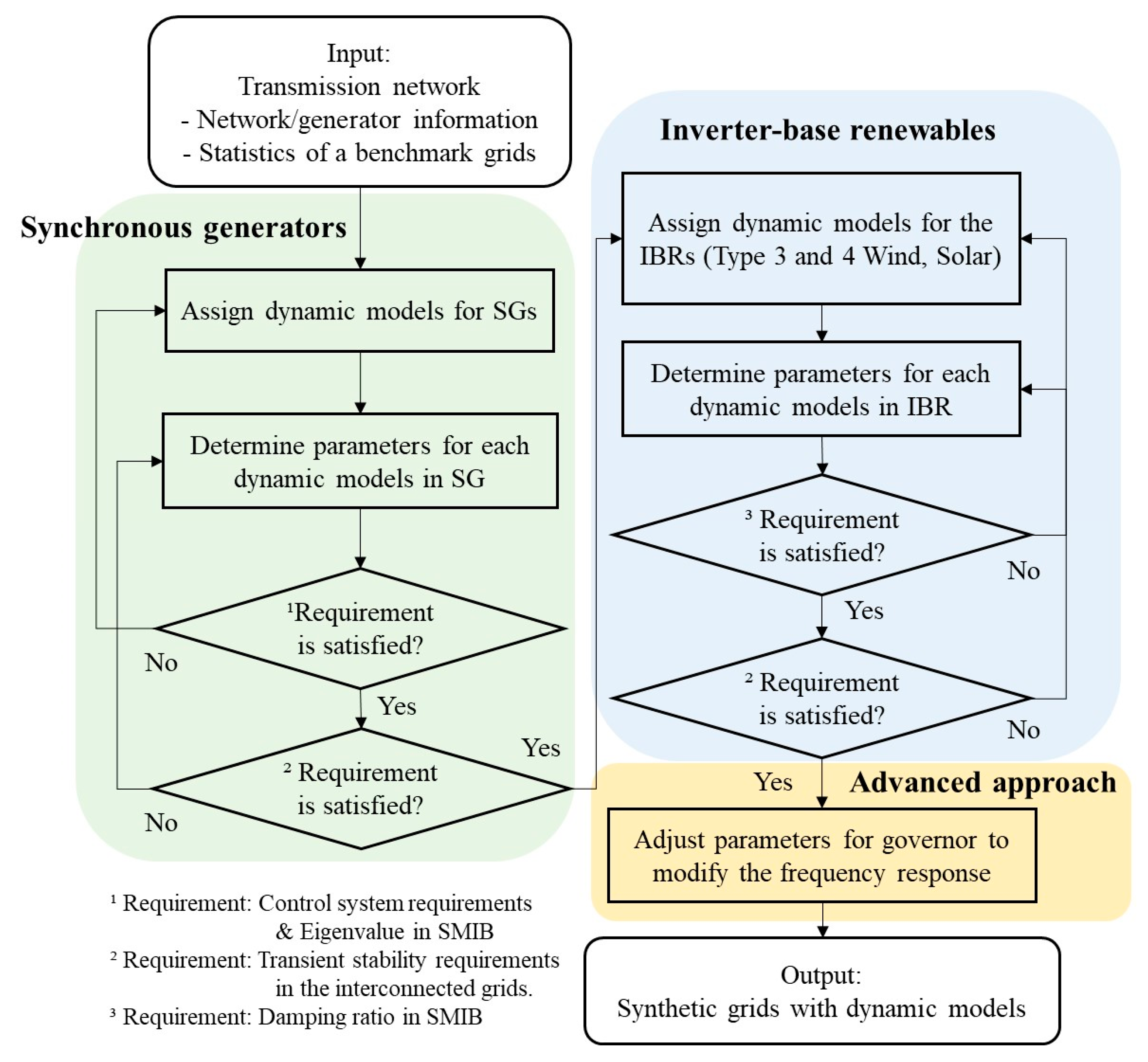
Figure 3 illustrates the automated algorithm for designing and validating dynamic models in synthetic grids. The algorithm integrates individual design and validation processes to improve flexibility and scalability across diverse transmission networks. It takes as input the synthetic transmission network data, including grid topology and generator-specific details such as fuel type, MVA rating, and MW/MVar limits [15]. A converged power flow solution is required at the starting operating point.

The process begins by selecting appropriate dynamic models for each generator based on its fuel type covering both SGs and IBRs. For each SG, the parameters of the machine, exciter, governor, and stabilizer models are determined using statistical data from actual benchmark grids, while also satisfying control system and individual model design requirements. Eigenvalue analysis in SMIB system is then conducted to ensure all generators exhibit stable dynamics. Subsequently, transient stability is evaluated in the full multi-machine system, with IBRs modeled as negative loads. If the system performance does not meet the predefined criteria, the algorithm iteratively reselects and adjusts the model parameters.

Following the validation of SG dynamics, IBR dynamic models are integrated into the system. Type 3 and Type 4 wind turbine models are selected based on statistical adequacy, while generic models are used for solar PV, and for both wind types. Small-signal stability analysis is then conducted for each IBR using SMIB system to guide parameter selection and ensure compliance with minimum damping ratio requirements. The transient response of the complete system, comprising both SGs and IBRs, is subsequently evaluated. If the system fails to meet the predefined stability criteria, the IBR model design and validation process is repeated iteratively until acceptable performance is achieved.

This paper introduces the concept of a system-wide governor model, a reduced-order model that captures the aggregate frequency response behavior of all governors in the system. By tuning the parameters of this model, the overall system frequency response can be adjusted to more closely reflect the realistic frequency behavior observed in benchmark systems.

Ultimately, the proposed framework produces synthetic grids incorporating validated dynamic models for both SGs and IBRs, facilitating reliable analysis of large-scale power systems with realistic dynamic behavior. Statistical analysis in this paper is done through comparison with a benchmark actual grid model consisting of a regional electric grid located in North America.

3.1. Frequency Response Control Design

3.1.1. Inertial/Immediate Frequency Response Control

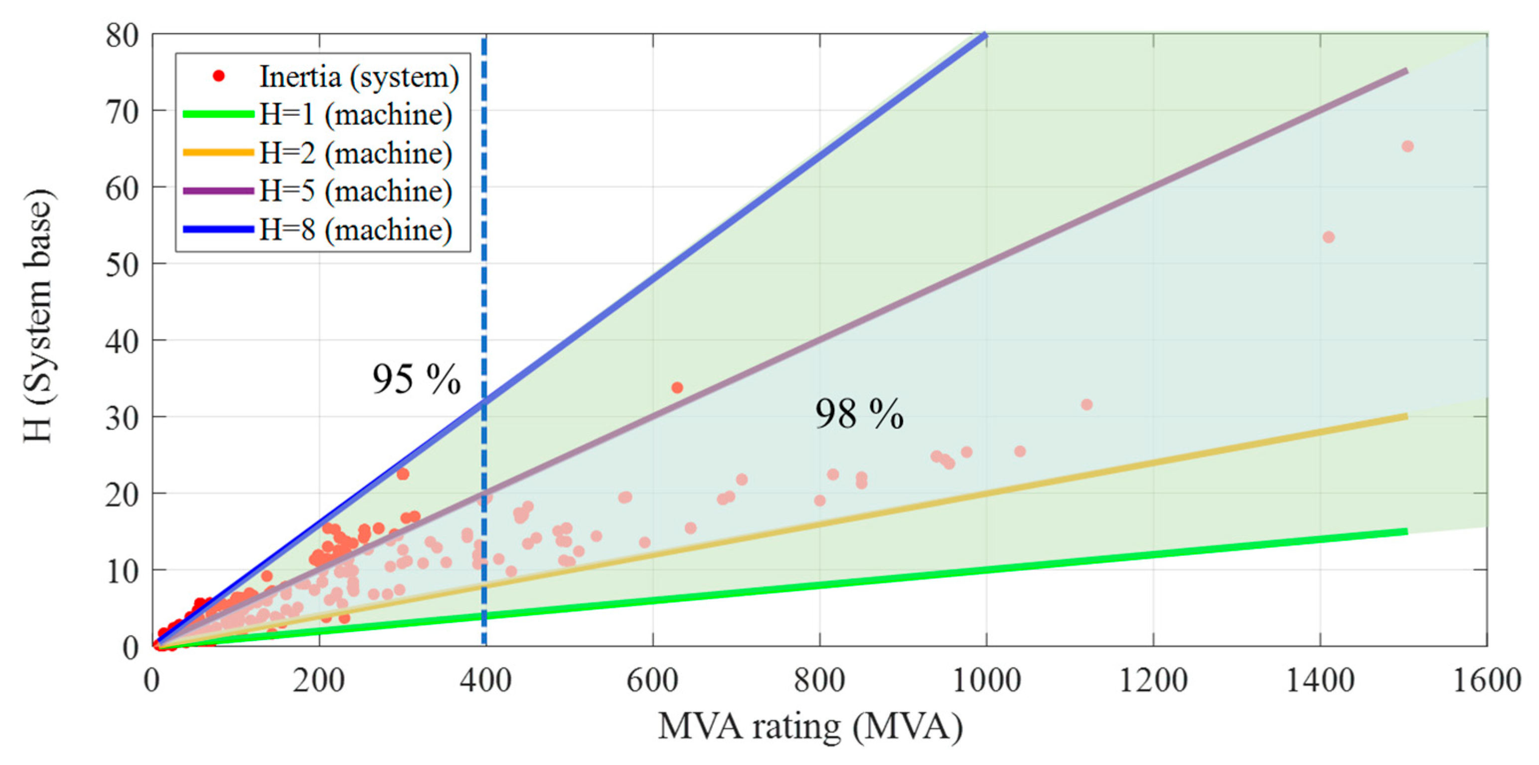
The transition of modern power grids highlights the importance of frequency stability. Frequency stability is closely related to the system inertia level during the inertial and immediate response. For example, the inherent absence of inertia in IBRs accelerates the RoCoF, which is a characteristic of inertial frequency response. Therefore, allocating the inertia to each generator is important to achieve a realistic frequency response.

For a realistic inertial response, inertia is assigned to generators based on the correlation between MVA rating and the inertia constant. An example of the GENROU machine’s relationship between inertia and MVA rating in the benchmark actual grids is illustrated in Figure 4. Red dots are the data of system-based inertia constants, and solid lines represent the guidelines of machine-based inertia. Among generators with an MVA rating smaller than 400 MVA, 95% have a machine-based inertia ranging between 1 and 8. Similarly, among generators with an MVA rating larger than 400 MVA, 98% have machine-based inertia ranging between 2 and 5. Inertia is determined within these boundaries. By defining system inertia within these limits, various levels of system inertia cases can be generated.

Additionally, the GFMs affect the inertial and immediate frequency response supporting system inertia and fault current. Reference [23] shows that frequency performance including RoCoF can be improved by GFMs, compared to the Grid Following Inverters (GFLs) in the grids. In synthetic grids, the GFM models can be included to study the impact of the transition for future power grids. The generic GFM models are available in the commercial power system software. For example, the PowerWorld simulator provides the REGFM_A1 model for GFM models [24].

The types of governor models and their parameters play a crucial role in the overall frequency response. The governor model is determined by the generator’s fuel type. In this paper, the IEEEG1, GGOV1, and HYGOV models are used as examples for steam, gas, and hydro turbines, respectively, following the recommended guidelines for typical planning studies in large interconnected systems [25]. Additionally, for realistic immediate frequency response, the turbine rating in governor models affect the limit for makeup power generation during contingency events. Therefore, the turbine rating for synthetic grids considers the statistics of the benchmark actual grids. The data for statistical analysis includes the active power capacity ($P_{max}$) of each generator, MVA rating ($S_B$), and turbine rating ($T_B$), showing the relationship: $P_{max}$≤ $T_B$ ≤ $S_B$. The normalized turbine rating, $T_{norm}$ is used to determine the realistic $T_B$. According to Equation (1), $T_{norm}$ equals zero when the $T_B$ matches the $P_{max}$ and equals one when the $T_B$ corresponds to the $S_B$.

$$T_{norm}={\displaystyle \frac{T_B-P_{max}}{S_B-P_{max}}}$$

(1)

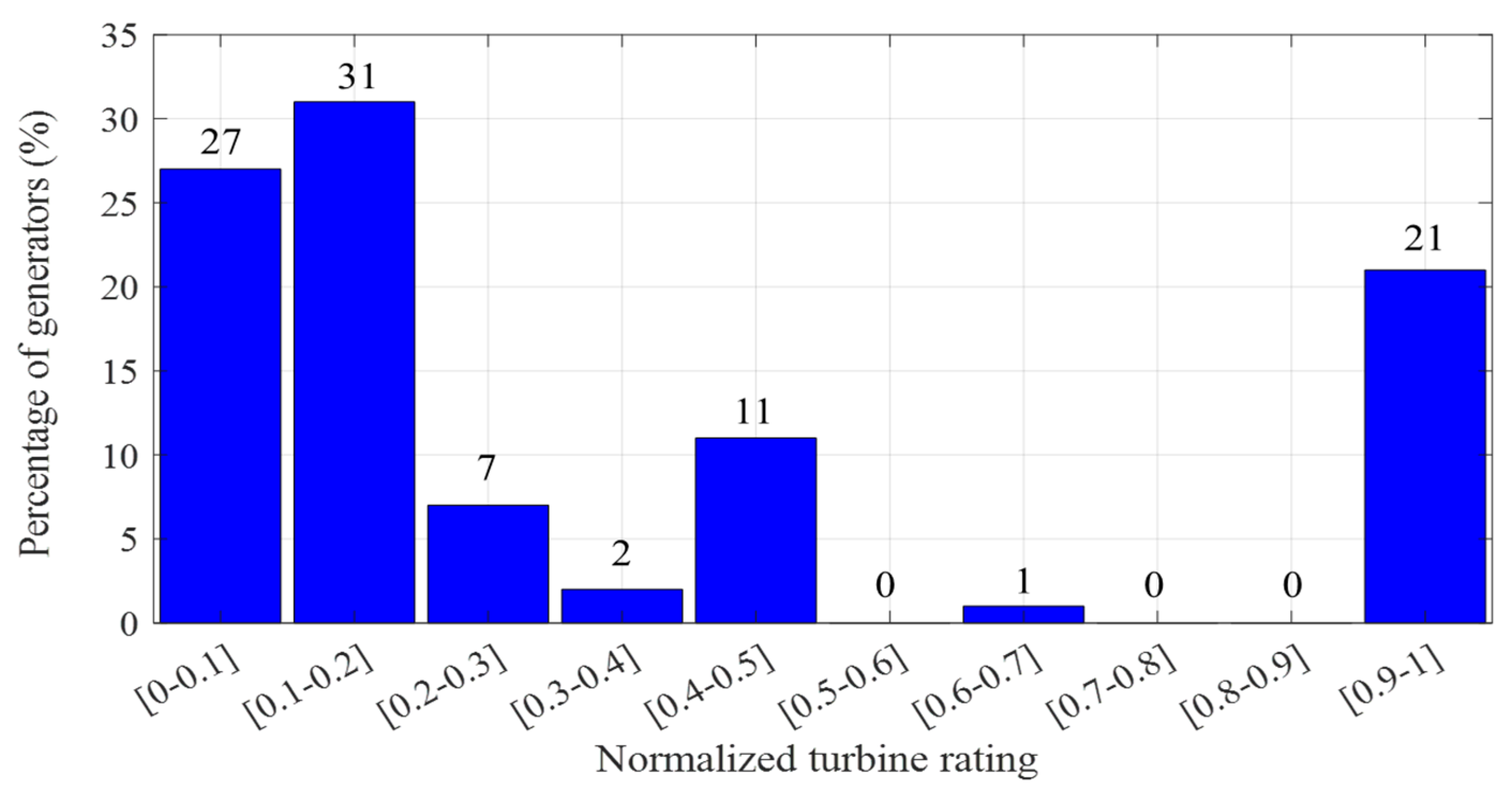
As an example, the GGOV1 model’s normalized turbine rating in the benchmark actual grids is shown in Figure 5. According to the result, 78% of generators have $T_{norm}$ between 0 and 0.46, and 21% of generators have $T_{norm}$ of 1.0, indicating that the turbine rating equals the $S_B$. The turbine rating in governor models for synthetic grids is determined by the probability of the statistical results.

3.1.2. Primary Frequency Response

In the primary frequency response, the settling frequency is determined by the droop constant in governor models. For a realistic primary frequency response, the droop constant must be determined carefully. For example, the droop constants of the GGOV1 model for synthetic grids are selected in the reasonable range between 0.03 and 0.05 by a uniform probability distribution considering the statistics in the benchmark actual grids and typical boundary.

Some parameters also highly affect the overall frequency response. The proportional gain ($K_p$) and integral gain $(K_i$) in gas turbine-governor models highly contribute to the overall frequency response. The impact of the increase of these PI gains ($K_p$, $K_i$) on the test grid is described in

Table 5. The impact of the increase in the gains of the gas turbine governor on frequency response.

Governor: GGOV1	Nadir [Hz]	Nadir Time [s]	Settling Time [s]
Increase of $K_p$	$+$0.03	$-$0.11	$+$4.39
Increase of $K_i$	$+$0.02	$-$0.71	$+$8.20
Increase of $K_p \& K_i$ (Constant $K_p/K_i$)	$+$0.05	$-$0.84	$-$2.30

which presents the sensitivity to PI gain variations. Each PI gain is increased by 50% relative to the sum of the current PI gains. As shown in the results, the impact on settling time is smallest when the ratio of $K_p$ to $K_i$ remains constant. To preserve similar settling time characteristics as those observed in the benchmark actual grids, this ratio is fixed to the average ratio obtained from the benchmark statistics. Within this constraint, $K_p$ is selected from a practical range between 1 and 10. Additionally, tuning methods based on the Ziegler–Nichols (ZN) approach can be applied for refining the gain values [26,27].

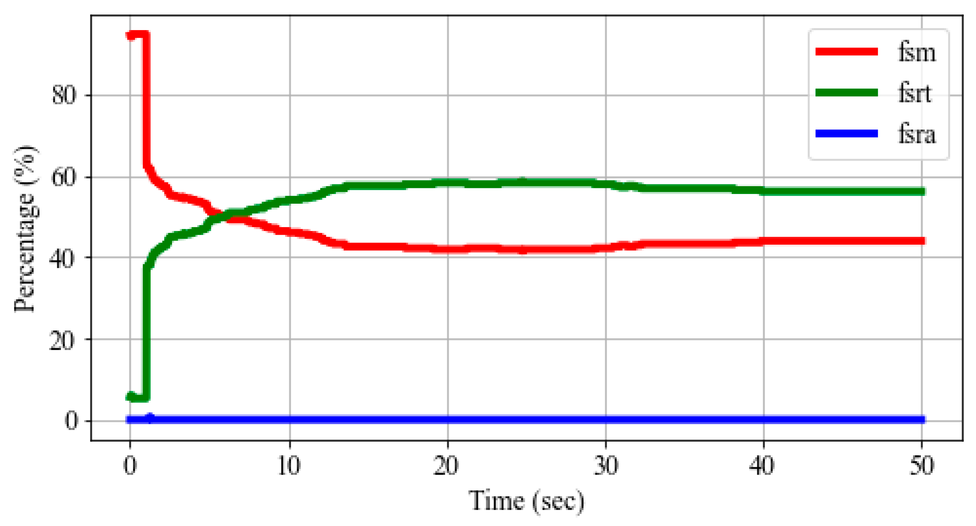
Specifically, the GGOV1 model uses three signals to control the valve position [25]. The first signal, “fsrn,” is the droop signal related to normal operation. The other two signals, “fsra” and “fsrt,” represent the acceleration controller and the temperature limit controller, respectively. The lowest value among the three signals is selected for the valve position. Figure 6 shows the percentage of generators exhibiting the lowest control signals in the test grids during a 50-s time-domain simulation following a generator outage event. As time progresses after the disturbance, the proportion of generators operating under normal conditions represented by the “fsrn” signal (red line in Figure 6) gradually decreases. In contrast, the percentage associated with the “fsrt” signal (green line in Figure 6), which corresponds to the temperature limit controller, increases. Specifically, the signal “fsrt” sets the limit based on the per unit maximum load value, as specified by the load limiter reference value. Analysis of the benchmark actual grids shows that the per unit limiter reference value is set to 1.0 for the large majority of gas turbine-governor models.

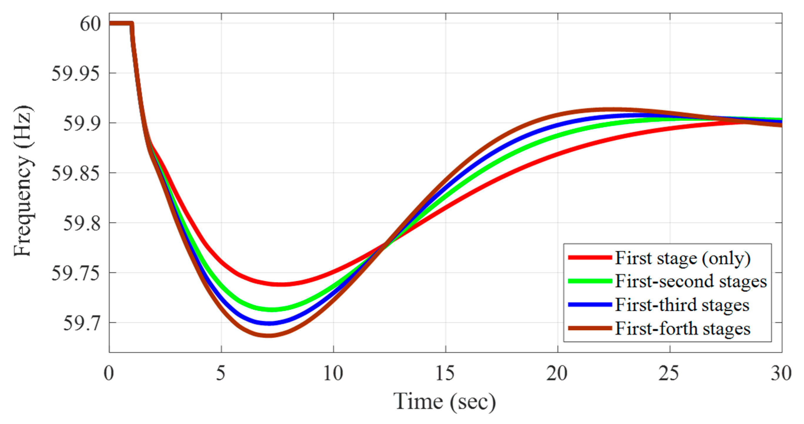
In steam turbine-governor models, steam stages are included to represent boiler dynamics. For example, the IEEEG1 model incorporates four steam stages: the steam chest and inlet piping, first reheater, second reheater, and crossover piping. In a full dynamic representation, these contributions are expressed through parameters, where $K_1$, $K_3$, $K_5$, and $K_7$ correspond to the high-pressure shaft, and $K_2$, $K_4$, $K_6$, and $K_8$ correspond to the low-pressure shaft. Figure 7 shows the indirect impact of the contribution of each stage on the overall frequency response illustrating the effect of the number of steam stages with a different distribution of $K_1$, $K_3$, $K_5$, and $K_7$ in the high-pressure shaft in the test grids. The results indicate that considering more stages leads to a lower frequency nadir and a faster settling time. To ensure realistic dynamic performance, the probability distribution of steam-stage contributions observed in the benchmark actual grids is incorporated into synthetic grids for the steam turbines.

3.1.3. Wide-Area Tuning with System-Wide Governor Model

Although the parameters in the dynamic models comply with the statistical characteristics of benchmark grids and satisfy stability requirements, the frequency response can be further refined to better reflect realistic system behavior. To address this, the paper employs a low-order model for system-wide governor design to understand the overall system dynamics. Several studies have focused on estimating system frequency trajectories using low-order models derived from governor behavior and system-level characteristics [28,29,30,31,32,33,34]. Based on these studies, this paper introduces a system-wide governor model that aggregates the influence of all steam and gas turbines in the system. Key parameters of this model are adjusted to approximate the desired frequency response observed in actual interconnected grids.

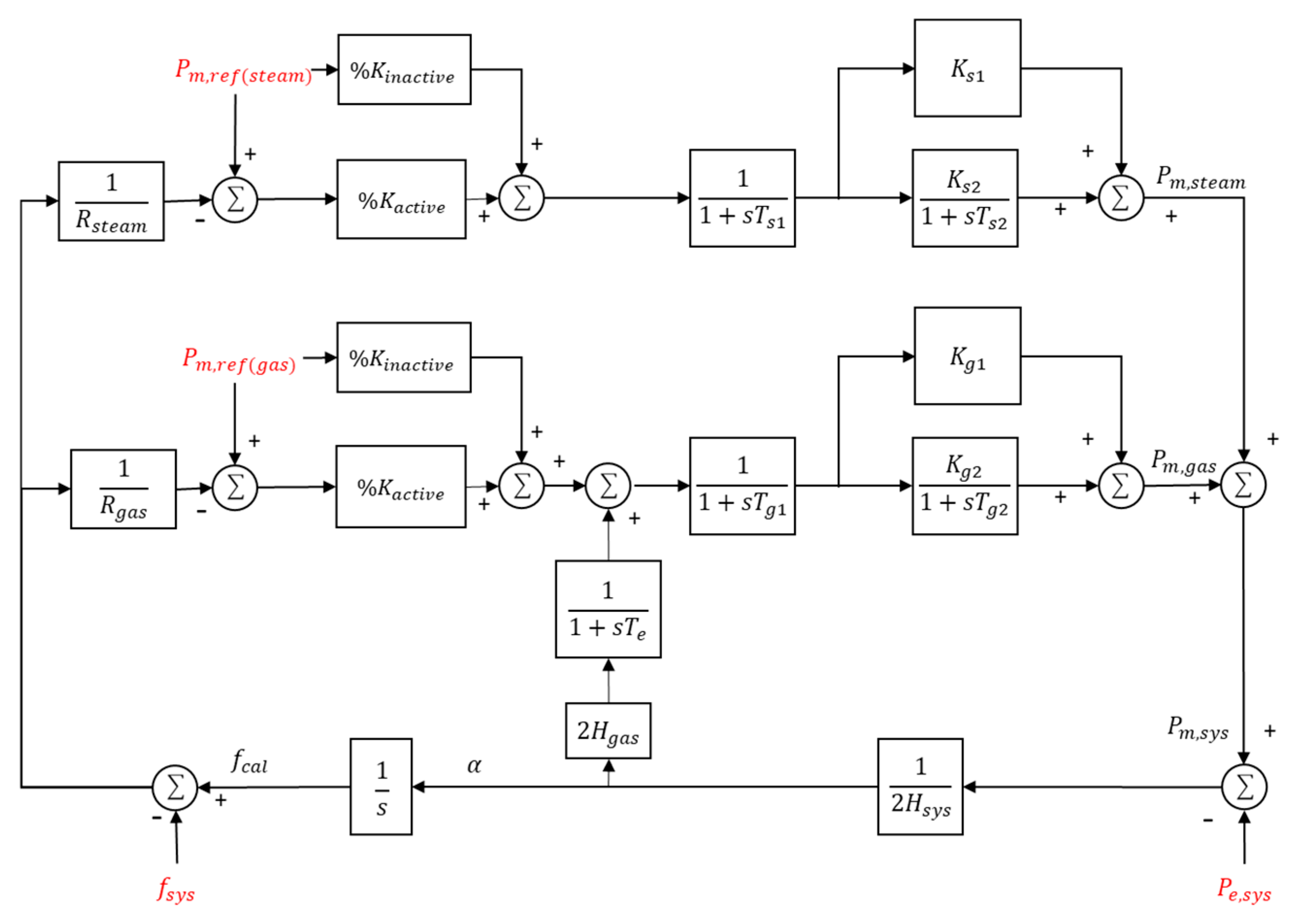
The system-wide governor model aggregates the behavior of gas and steam turbines, incorporating droop control, fast response, and slow response components. Each part is represented as Equations (2)–(5), where $P_{m,ref}$ is the sum of the reference powers in each model, ${\omega }_{sys}$ is the system’s nominal frequency, $R$ is the aggregated droop constant, $T_1$ and $T_2$ are the fast and slow time constants, $K_1$ and $K_2$ are proportional gains for fast and slow response.

• Droop control:

$$v=-({\omega }_{sys}-\omega )/R+P_{m,ref}$$

(2)

• Fast response:

$$\dot{x_1}=(v-x_1)/T_1$$

(3)

• Slow response:

$$\dot{x_2}=(x_1-x_2)/T_2$$

(4)

• Mechanical power:

$$P_m={K_{1}x}_1+K_2{x}_2$$

(5)

Based on Equations (2)–(5), Figure 8 presents the aggregated block diagram of the system-wide governor, illustrating how it captures both the system frequency response and the mechanical power response during disturbances. In this model, $P_{e,sys}$ represents the total electrical power from the time-domain simulation, and $P_{m,ref\left(steam\right)}$ and $P_{m,ref\left(gas\right)}$ correspond to the total mechanical reference power of steam and gas turbines, respectively. The system nominal frequency is denoted as $f_{sys}$, $H_{gas}$ is the aggregated inertia from gas turbines, and $H_{sys}$ is the system inertia constant.

The model includes nine tunable parameters associated with droop, time constants, and gain values. These parameters are listed in

Table 6. The description of parameters in the system governor.

$R_{gas}$	Droop for gas turbine
$R_{steam}$	Droop for steam turbine
$T_e$	The time constant for the measurements of $P_e$
$T_{g1}$	The fast time constant for gas turbine
$T_{g2}$	The slow time constant for gas turbine
$T_{s1}$	The fast time constant for steam turbine
$T_{s2}$	The slow time constant for steam turbine
$K_{g1}$	The ratio of the fast response of gas turbine
$K_{s1}$	The ratio of the fast response of the steam turbine

and are tuned by minimizing the error between the system frequency response from the time-domain simulation and its approximation using the model. Furthermore, generator limits are represented in the model through the parameter $\%K_{inactive}$, which denotes the percentage of generators that reach their maximum active power output in the power flow solution.

Once the initial parameters are determined, they can be further adjusted to modify the system’s frequency response characteristics. Since the parameters in the system-wide governor model do not correspond directly to those of individual generators in the original system, a multiplier is introduced for tuning. For example, to achieve a slower system frequency response, the time constants in the system-wide model can be increased by a chosen multiplier. This same multiplier is then uniformly applied to the corresponding parameters in the full dynamic system to ensure consistent behavior. An illustration of this approach is shown in Figure 9 using a large-scale test grid (the Texas 2000-bus case). In this example, a multiplier of 1.5 is applied to the time constants of all steam turbine governors in test case to slow down the frequency response. The figure compares the base frequency response of the original system (red line) with the refined responses obtained from both the full simulation and the approximation using the system-wide model (green and blue lines, respectively). This example demonstrates that a full dynamic simulation is not required to iteratively adjust the multiplier in order to achieve the desired frequency characteristics. Instead, the system-wide governor model is able to be used to capture and adjust the system frequency dynamics. Consequently, this approach can contribute to more intelligent simulation for frequency stability.

3.2. Voltage Control Design

This section introduces the design method for exciters and IBRs considering the statistical data, small-signal stability, and transient stability to achieve realistic voltage performance in synthetic grids.

Exciters in SGs are crucial to voltage control performance, as they regulate rotor field current to maintain or restore voltage during and after contingencies. Various exciter models have been developed, and several are currently used in modern power grids. In [16], the exciter models used in actual grids are categorized based on the fuel type of generators. This paper adopts the commonly used exciter models identified in the benchmark actual systems.

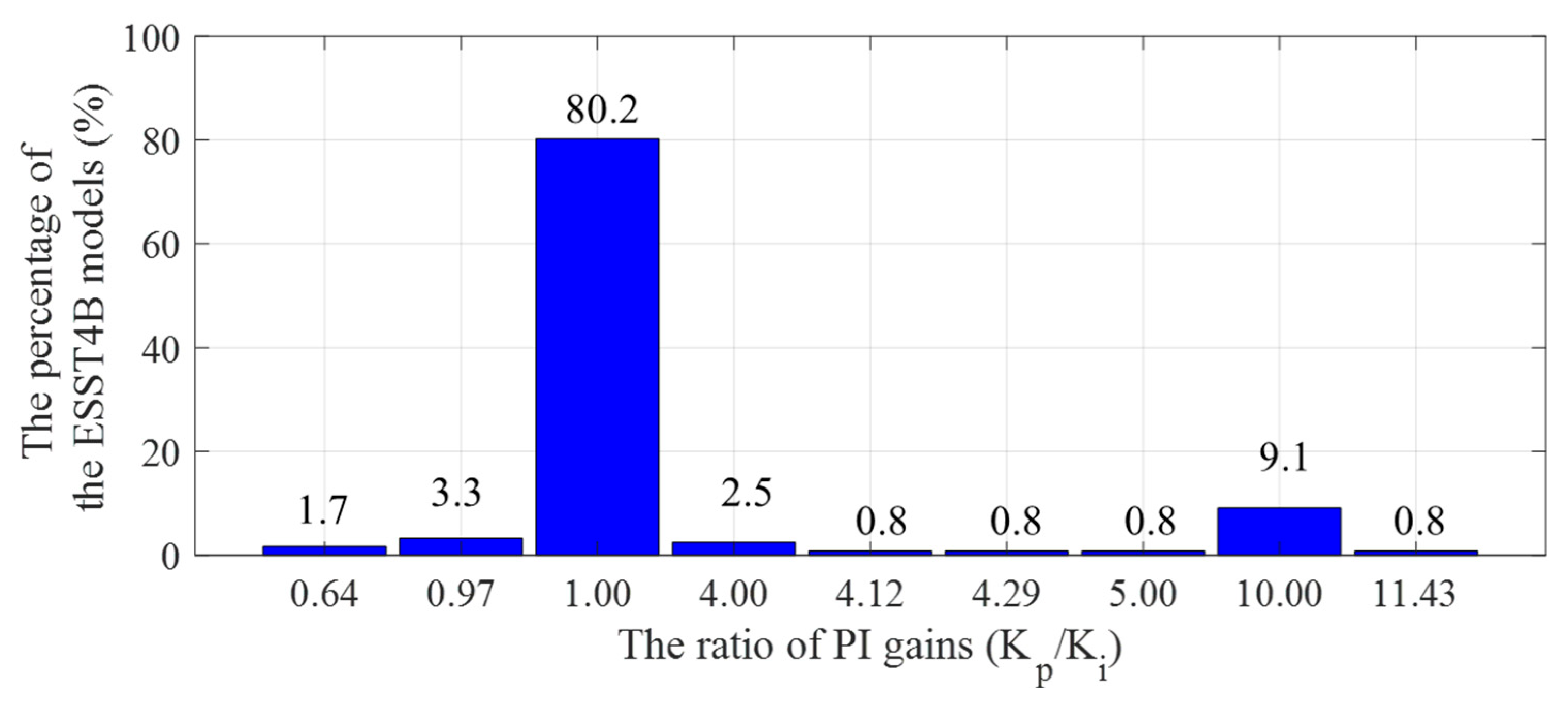
Each exciter model features distinct control mechanisms, such as lag-lead filter, rate-feedback, or PI control. The control structures used in each model are analyzed based on statistical studies from the benchmark grid. For instance, although the generic ESST4B model allows for a dual-PI configuration, all ESST4B models observed in the benchmark actual grids utilize a single PI control loop. Additionally, 80% of these ESST4B models use identical proportional and integral gains, as shown in Figure 10.

The increase in the penetration of IBRs results in a weaker transmission network, reducing the short-circuit current, which is crucial for maintaining voltage during contingencies [35]. Hence, IBRs should be designed well to effectively study voltage control in future grids with high IBR penetration.

The generic models for IBRs and their combinations have been developed for positive sequence simulation and discussed in [36,37,38], depending on whether the generation is from solar, Type 3 wind, or Type 4 wind. The adequacy of Type 3 and Type 4 wind turbines based on their MVA rating in actual grids is illustrated in Figure 11 [19].

The initial parameters of IBRs for synthetic grids are determined using the generic models, their combinations, and the statistical results from the previous study in [19]. The parameters are validated in the small-signal stability and transient stability perspectives.

From the perspective of small-signal stability, it is imperative to note that each IBR must exhibit adequate damping. To achieve this, small-signal analysis is employed in the IBR model using the SMIB system. The parameters of each IBR are validated to have a satisfactory damping ratio through small-signal analysis.

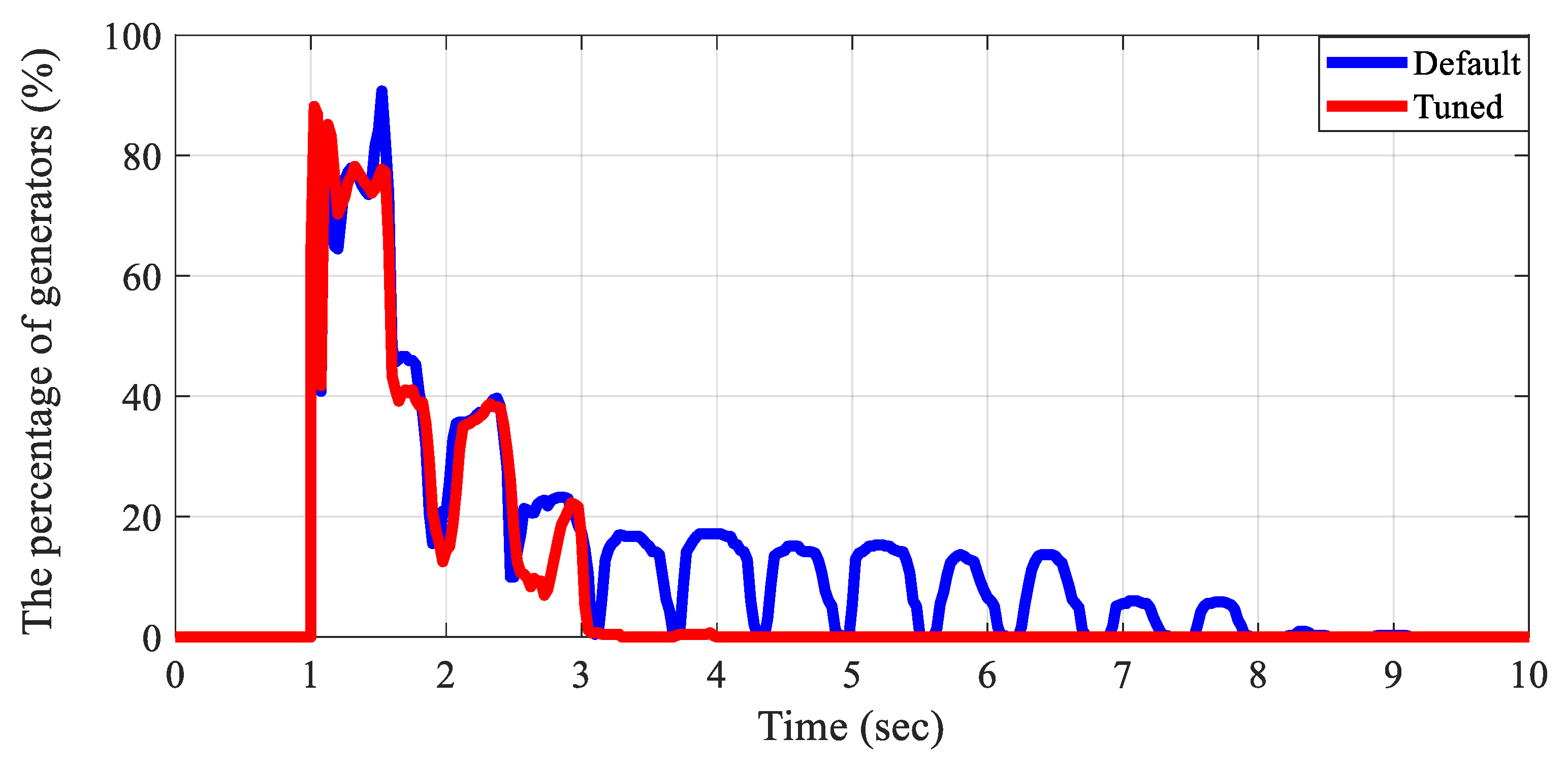
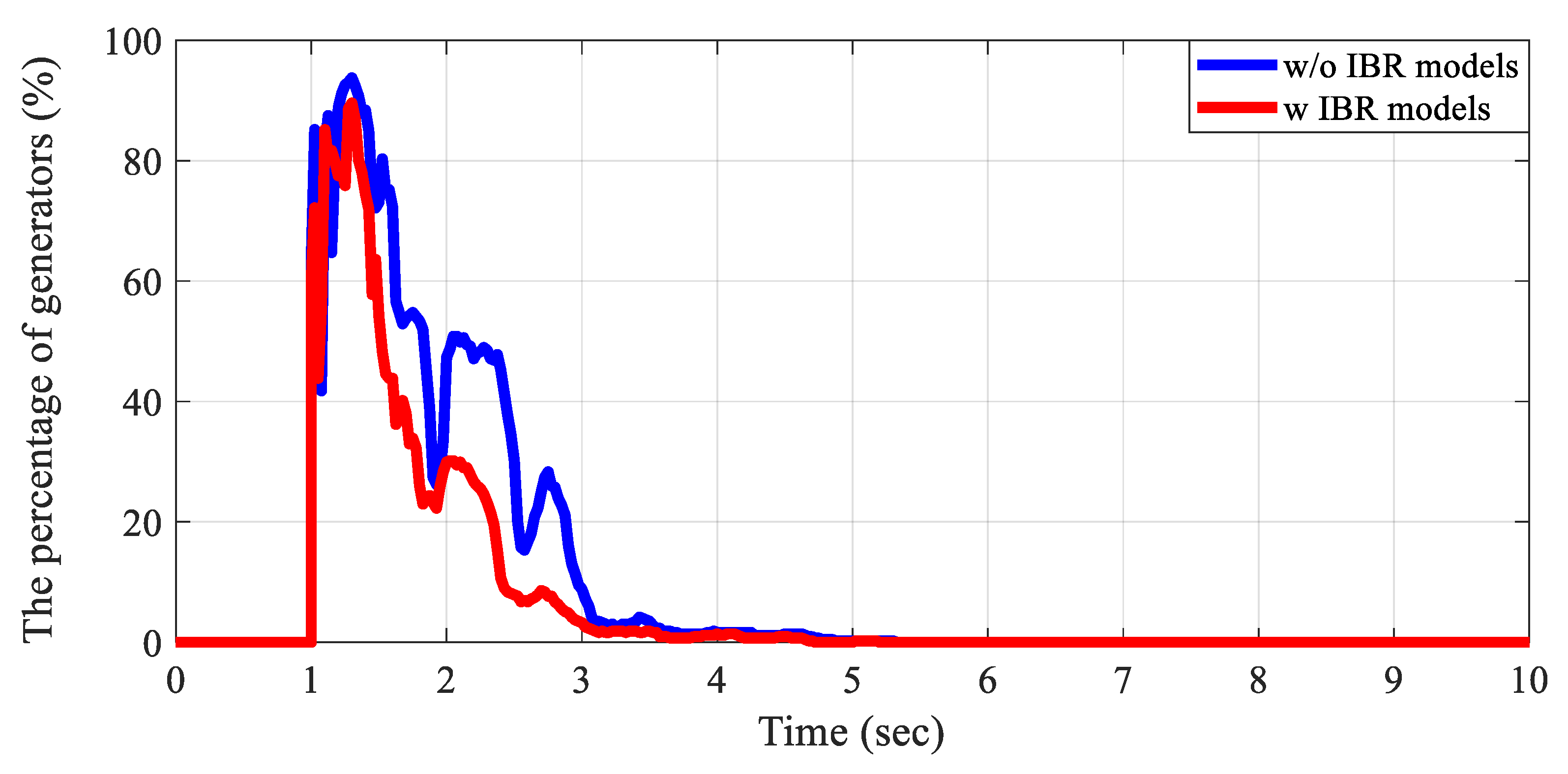
The exciter and IBR models, along with their parameters, are further validated through the transient stability perspective under event conditions. Figure 12 demonstrates that the exciter tuning process in the interconnected test grid improves the system’s ability to maintain synchronism and restore voltage to its operating point after a contingency. The percentage of generators exhibiting a voltage deviation greater than 0.5% from the operating voltage is analyzed under a solid three-phase balanced fault and clear scenario. When using the default parameters suggested by a commercial tool for the exciter models, oscillations are observed, and all generators converge to the operating point 8–9 s after the fault. Otherwise, after tuning the exciters, every generator converges to the operating point within 3 s after the fault. Similar to exciter validation, the IBR dynamic models in the interconnected test grid are validated through scenarios that compare voltage responses without and with tuning IBR dynamic models under the same contingency. In the case without IBR dynamic models, IBRs are assumed to be negative loads in the dynamic simulation. As shown in Figure 13, IBR dynamic models help the voltage performance converge to the operating points faster.

3.3. Oscillation Response Design

The presence of poorly damped oscillations within interconnected large power systems poses a serious risk of blackout. To mitigate these oscillations and enhance system stability, Power System Stabilizer (PSS) and its tuning methods have been extensively studied over the past decades [39,40,41].

In this paper, the PSS2A model is used for synthetic grids as a sample. For this model, the time constants in the lead-lag blocks are tuned to achieve well-damped oscillations in the SMIB system. Additionally, to reflect the response speed of the PSS in an actual grid, statistics for other parameters are included. For example, 99% of PSS2As in actual grids have the same $T{w}_1$, $T{w}_2$, $T{w}_3$, and $T_7$ values within the range between 2 and 15. The gain $K_2$ would be equal to $T_7/2H$ where $H$ is shaft inertia in machine-base [22]. Furthermore, the gain $K_1$ is tuned based on the result of the eigenvalue analysis of the SMIB system. 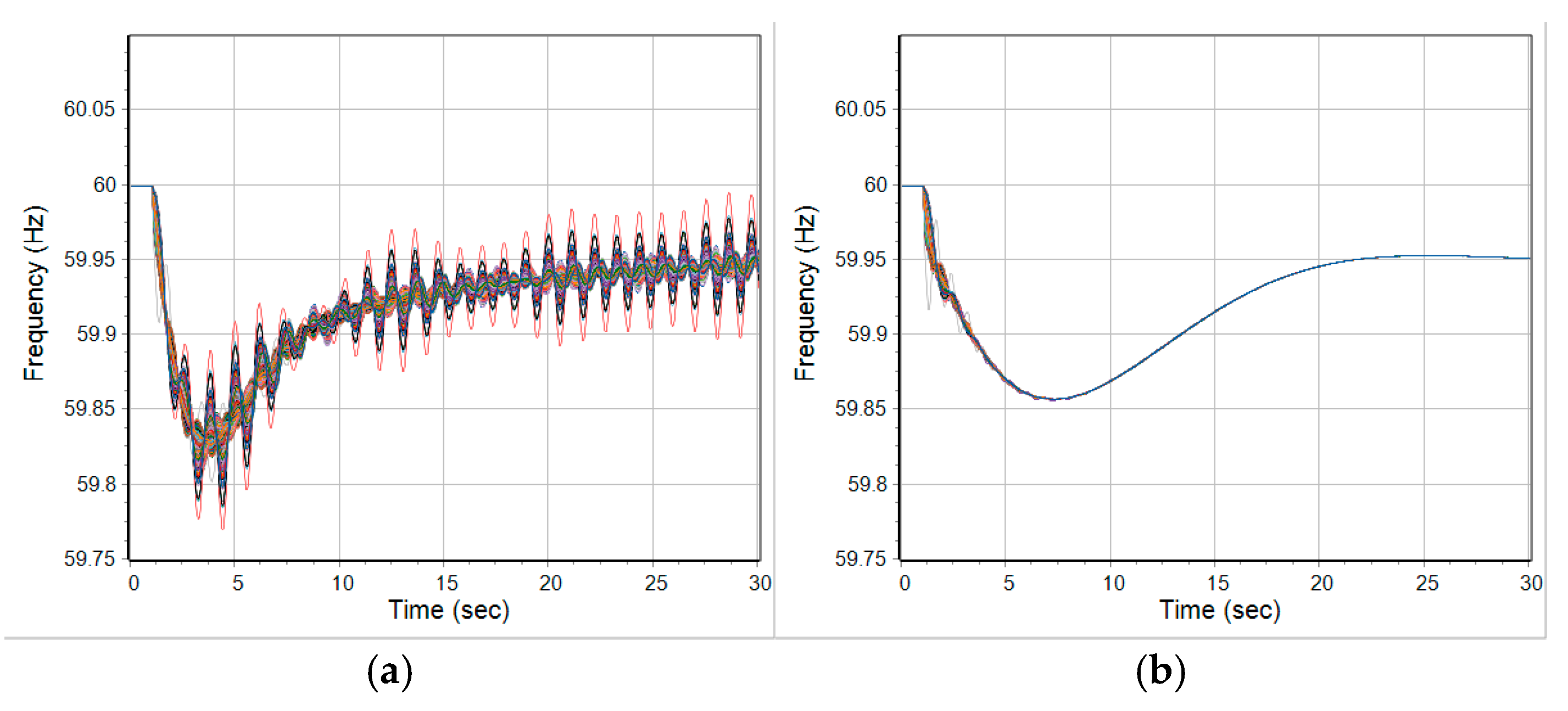For illustrations, Figure 14 shows the improvement of oscillation response without and with tuning stabilizers in the test case.

4. Result and Analysis on 2000-Bus Cases

This section gives the analytical results derived from the 2000-bus case models introduced in Section 2. The dynamic models for five different Texas synthetic grids, listed in Table 2, are developed based on statistical data from a benchmark actual grid and on the stability requirements defined at the model, generator, and system levels.

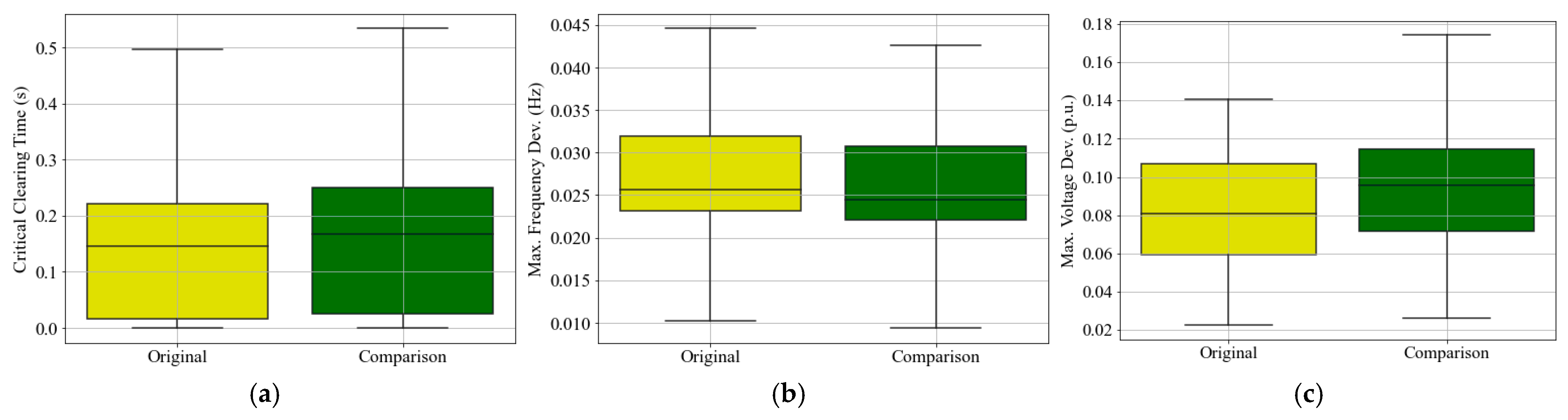
As an initial validation step, two distinct dynamic models are generated for the same scenario (Base) to assess the statistical consistency in dynamic performance. Figure 15 compares the performance of these two models under a filtered N-1 contingency, focusing on generator speed, system frequency, and voltage stability. In the box plots, the upper and lower whiskers represent the maximum and minimum values for each metric, while the boxes indicate the first and third quartiles, with the median marked inside the box. Figure 15a presents a box plot of the critical clearing times (CCT) across 120 scenarios involving three-phase bus-to-ground solid faults. CCT represents the maximum fault duration the system can withstand before any generator loses synchronism. The close alignment between the two models in both median and interquartile range indicates consistent transient stability margins across fault locations. Figure 15b shows the statistical distribution of the maximum system frequency deviations across 113 N-1 generator outage scenarios. This metric reflects the system’s inertial response and primary frequency control, capturing the frequency nadir after each outage. The similarity in statistical distribution between the two models indicates consistent frequency performance and adequate frequency control. Figure 15c illustrates the maximum terminal voltage deviations of generators in response to 120 three-phase bus-to-ground faults cleared after three cycles. Voltage deviation serves as an indicator of voltage stability and excitation system response. The box plots confirm that both models exhibit similar voltage regulation behavior under fault conditions. Overall, the results in Figure 15 demonstrate that the two different dynamic models, constructed using the same statistical assumptions and stability constraints, produce statistically consistent system responses across rotor angle, frequency, and voltage metrics. This validates the reproducibility and robustness of the synthetic grid development framework.

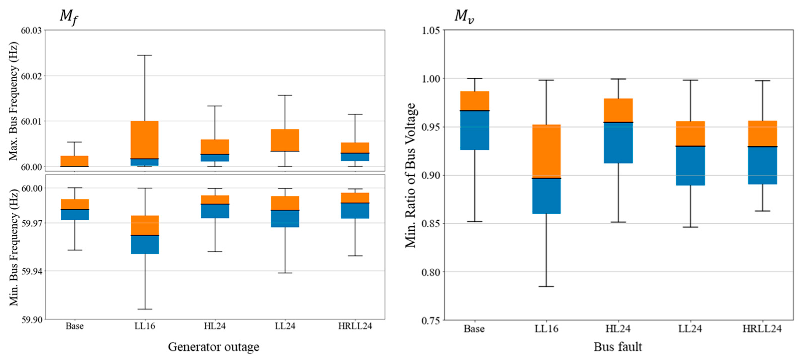
The dynamic performance of the five cases is evaluated using transient stability metrics specified in prior reports [42,43]. These metrics include the minimum and maximum bus frequency values ($M_f$), as well as the minimum ratio of bus voltage to its pre-contingency level ($M_v$). The specific performance requirements are summarized in

Table 7. Transient stability metric requirements.

Metric	${\mathit{M}}_{\mathit{f}}$	${\mathit{M}}_{\mathit{v}}$
Requirement	[59.5, 60.5] Hz	0.75

[17]. Two types of N-1 contingencies are analyzed: generator outages (for frequency evaluation) and bus faults (for voltage performance). For the bus fault scenarios, a three-phase solid fault is applied and cleared after three cycles. Full dynamic simulations are conducted for each N-1 contingency across the five cases, and the corresponding transient stability metrics are computed. Figure 16 presents box plots summarizing the statistical results of the N-1 contingency analysis. The results confirm that the dynamic performance of all five cases satisfies the defined stability requirements.

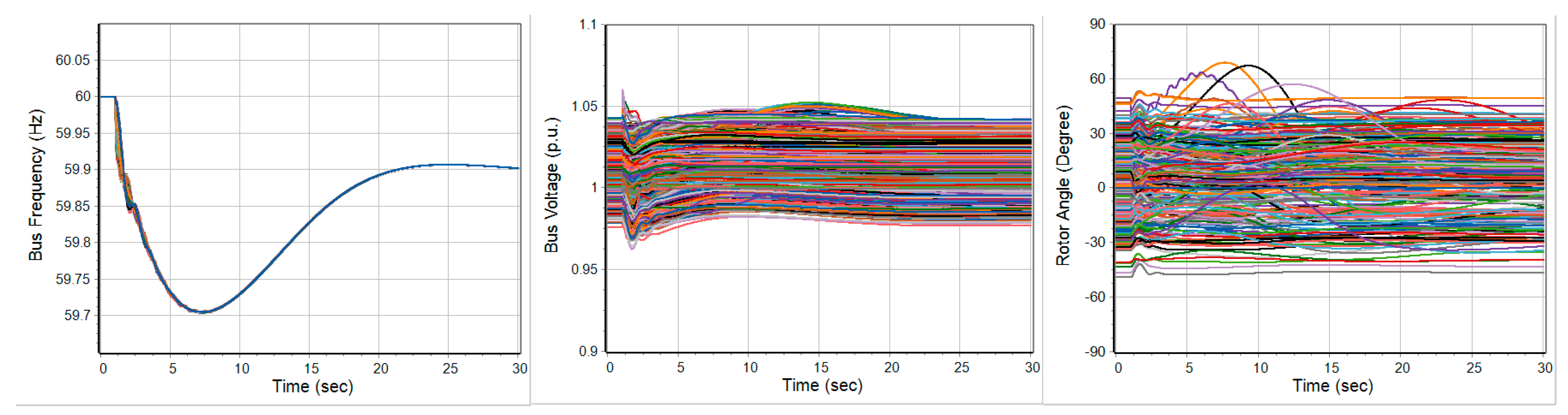
The dynamic performances are validated under a severe contingency involving the outage of the two largest generators, resulting in a total generation loss of 2708 MW. The simulation result of Base case with the bus frequency, bus voltage, and rotor angle profile are illustrated in Figure 17. The transient stability metrics indicate a well-behaved system response: the frequency stability metric $M_f$ remains within the acceptable range of [59.7, 60] Hz, and voltage stability metric, $M_v$ is 0.97, confirming a stable frequency and voltage recovery satisfying the requirements in Table 7. Notably, the average bus frequency response after the same contingency in five cases was illustrated in Figure 2 and Table 3, demonstrating robust system-wide performance under severe event.

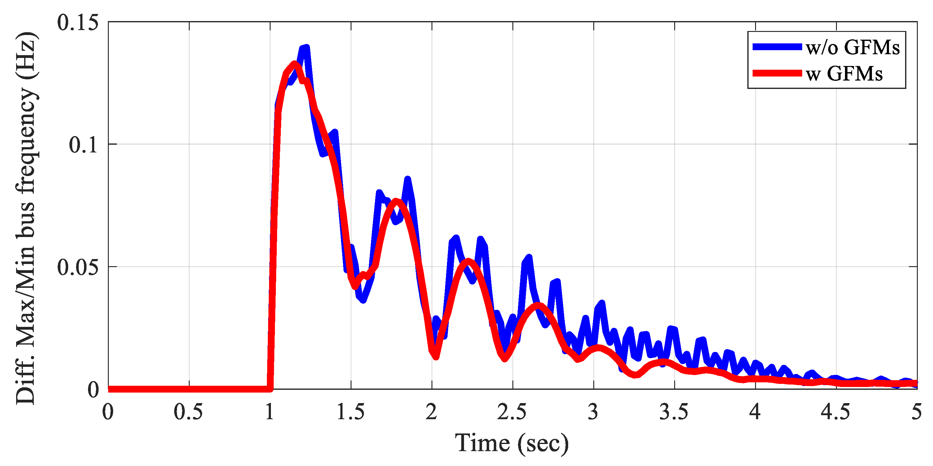
Although all cases show stable frequency responses, increasing the generation of IBRs while de-committing SGs weakens the grid stability under contingency situations. In LL24 case, which represents an IBR-heavy and low-inertia scenario, high frequency oscillations occur after the contingency. As a solution, GFMs can improve stability in an IBR-heavy grid. In Figure 18, the difference between the minimum and maximum bus frequencies at each time point illustrates the high frequency oscillations in LL24 case and the mitigated oscillations with the addition of GFMs. Notably, only two GFMs (MVA rating: 100 MVA) are added to the IBR-heavy area.

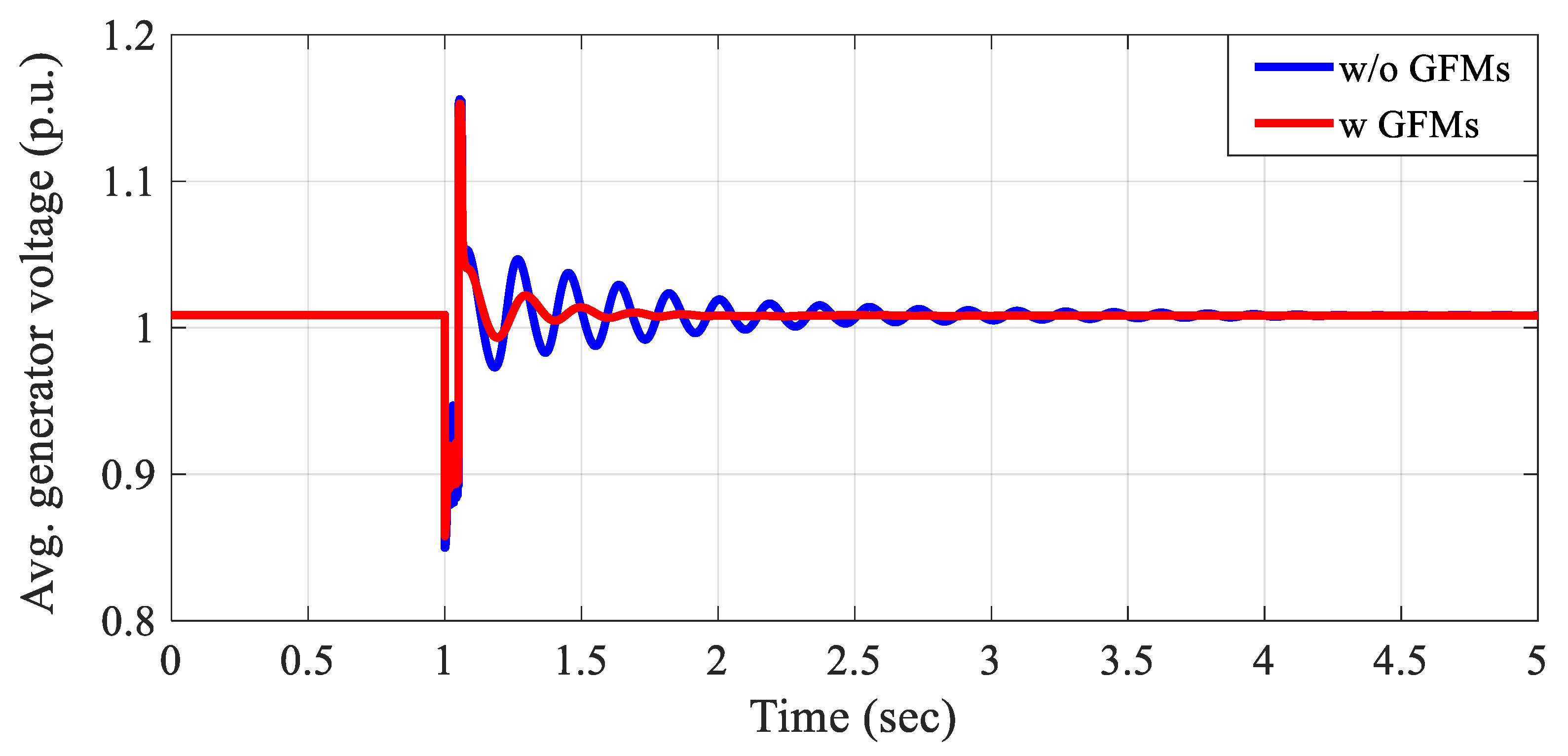
The voltage performance is validated using the time-domain simulation. When the solid three-phase fault to a bus scenario is applied to the test cases, all generators recover their voltage to the operating point after clearing the fault. However, in the weak grid, such as LL24 case, poorly damped oscillation is observed in the voltage response, as shown by the blue line in Figure 19. Similar to the frequency study findings, the integration of GFMs improves system stability. As shown by the red line in Figure 19, the GFMs effectively mitigate oscillations, resulting in a faster and more stable voltage recovery in weak grid conditions.

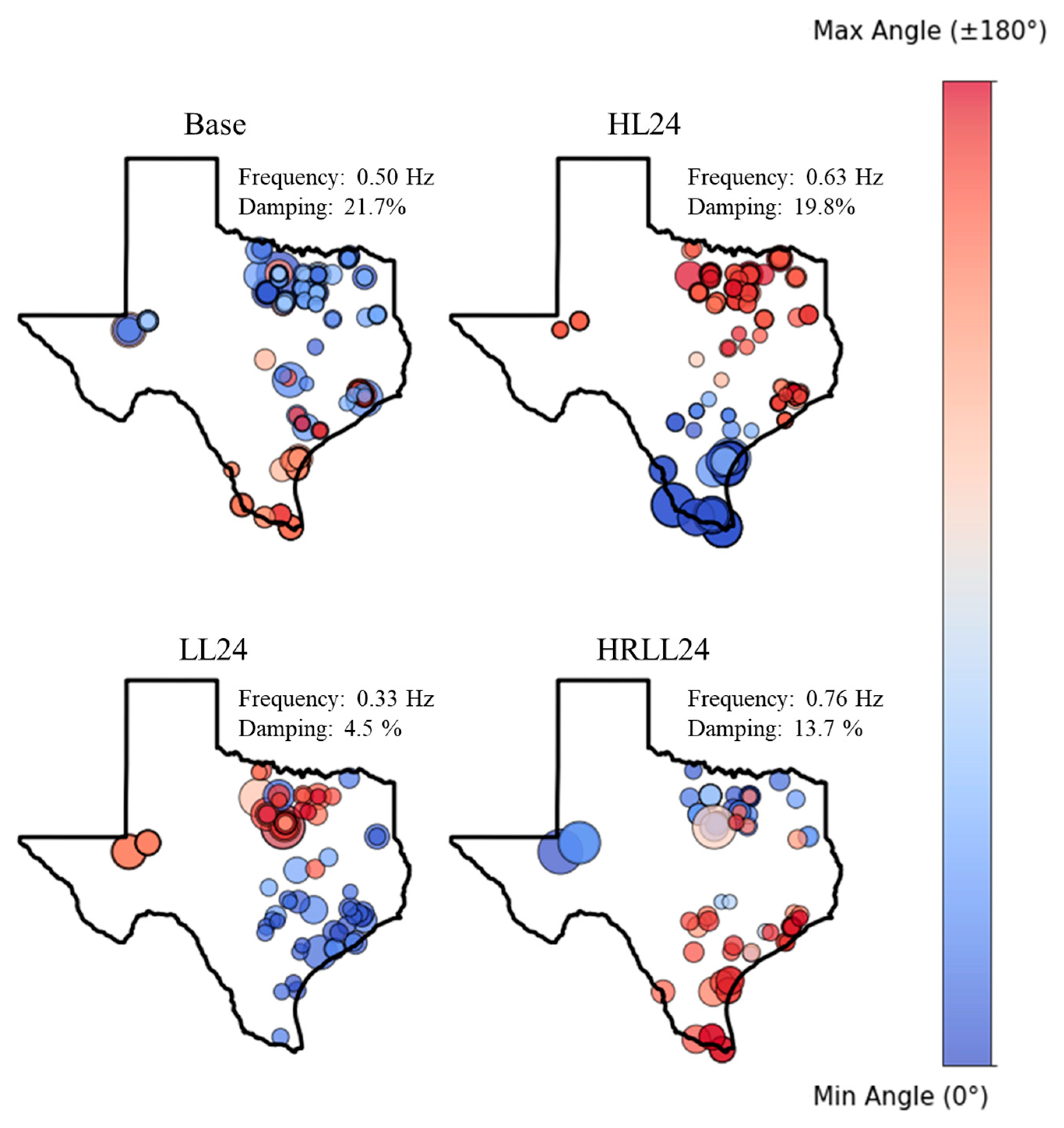
Using the test cases, inter-area oscillations in the Texas synthetic grids are studied. To extract the oscillatory modes, the Iterative Matrix Pencil method is employed within the PowerWorld Simulator. In LL16 case, there is no clear inter-area mode, but the other cases show a distinct inter-area mode related to the north and south areas. These inter-area modes are illustrated in Figure 20. The size of the circle represents the relative magnitude of the mode, while the color indicates the angle of the mode. LL24 case’s inter-area mode has the smallest damping at 4.5% with a frequency of 0.33 Hz, while the other cases have sufficient damping, greater than 10%.

5. Discussion and Conclusions

This paper introduces a comprehensive framework for designing and validating the dynamic performance of SGs and IBRs in synthetic power grids. To achieve realistic dynamic performance, the statistical relationship of parameters within the generator dynamic model is derived from benchmark actual grid models. Additionally, characteristics of power system stability—including frequency, voltage, and oscillations—and control system theory are considered in the overall parameter determination process. Furthermore, a concept of system-wide governor design is used in this paper to simplify the adjustment of the governor parameters. The processes introduced in this paper are integrated into an automated algorithm.

The process of designing comprehensive SGs and IBRs to achieve dynamic performance enhances the performance of synthetic grids, making them more realistic. Introducing system-wide governor design improves controllability in the frequency response of synthetic grids. Furthermore, automated algorithms increase flexibility in generating synthetic dynamics across various transmission networks. To reduce the need for manual adjustments in achieving a reasonably stable response, this paper proposes a structured and modular validation framework comprising three levels: individual model validation, individual generator validation, and overall system performance validation. This framework enables the systematic design of a stable dynamic response at each level. These benefits lead to the development of test cases to validate performance under different conditions, including high/low-load and high/low-inertia scenarios. In all cases, dynamic performances demonstrate stable responses converging to equilibrium points in all N-1 contingencies and a largest N-2 generator event. In the case, characterized by IBR-heavy and low-inertia systems, high frequency oscillations are observed. Installation of GFMs in IBR-heavy areas effectively mitigates these oscillations. Additionally, studying inter-area oscillations demonstrates that IBR-heavy and low-inertia conditions worsen the damping of inter-area modes.

This paper generates diverse, realistic synthetic grid cases. Through advanced synthetic grids, researchers and engineers can freely explore envisioned future power grids, and they can share the results for cross-validation. Consequently, this paper supports grid planning by identifying the potential impacts of the transition to future power grids.