Model Predictive Control for Charging Management Considering Mobile Charging Robots

Abstract

Mobile Charging Robots (MCRs), essentially high-voltage batteries mounted on mobile platforms, offer a flexible solution for electric vehicle (EV) charging, particularly in environments like supermarket parking lots with photovoltaic (PV) generation. Unlike fixed charging stations, MCRs must be strategically dispatched and recharged to maximize operational efficiency and revenue. This study investigates a Model Predictive Control (MPC) approach using Mixed-Integer Linear Programming (MILP) to coordinate MCR charging and movement, accounting for the additional complexity that EVs can park at arbitrary locations. The performance impact of EV arrival and demand forecasts is evaluated, comparing perfect foresight with data-driven predictions using long short-term memory (LSTM) networks. A slack variable method is also introduced to ensure timely recharging of the MCRs. Results show that incorporating forecasts significantly improves performance compared to no prediction, with perfect forecasts outperforming LSTM-based ones due to better-timed recharging decisions. The study highlights that inaccurate forecasts—especially in the evening—can lead to suboptimal MCR utilization and reduced profitability. These findings demonstrate that combining MPC with predictive models enhances MCR-based EV charging strategies and underlines the importance of accurate forecasting for future smart charging systems.

1. Introduction

Mitigating greenhouse gas emissions is essential to achieving the climate targets set out in the Paris Agreement. This necessitates a fundamental transformation of the mobility, transport, and energy sectors. The growing relevance of electric mobility (E-mobility) is already becoming apparent [1]. A central challenge in this context is the planning, deployment, and operation of charging infrastructure. Users expect charging solutions to be reliable, user-friendly, and fast, whereas charge point operators (CPOs) aim to maximize the profitability and efficiency of their infrastructure investments. At the same time, grid operators are tasked with maintaining grid stability amid increasing electricity demand. The growing adoption of electric vehicles (EVs) highlights the significance of public charging infrastructure. According to the International Energy Agency [2], public charging solutions are expected to play a crucial role to establish E-mobility and enhance user acceptance. These solutions are designed to complement existing home and fleet charging options, catering to the needs of EV users in urban and high-traffic areas. Various approaches have been proposed to account for the diverse interests of stakeholders. Intelligent charging strategies (such as smart and bidirectional charging) are gaining prominence in fleet management and home charging scenarios. In public and semi-public settings, battery storage concepts are increasingly utilized to minimize the need for grid reinforcement while still delivering high charging power and fast charging capabilities. However, a fundamental challenge remains: although charging solutions supported by stationary storage provide flexibility to the grid, they do not offer the same level of flexibility to users. In the event that all charging ports are in use, users may be required to return at a later time.

The implementation of Mobile Charging Robots, such as the GINI robot presented by Wessel et al. [3], offers numerous benefits when compared to stationary solutions. These mobile robots enhance flexibility in charging location, potentially improving user satisfaction by reducing wait times and optimizing charging infrastructure utilization. Furthermore, they can assist in balancing the load by charging their own batteries during off-peak hours and discharging stored energy during periods of high demand, thereby reducing grid strain. On the downside, deployment of MCRs increases investment and operation costs in comparison to stationary alternatives. While such systems have the potential to increase revenue by serving a greater number of vehicles, the financial viability of these systems must be carefully assessed.

Faßbender et al. [4] introduced a simulation environment that models charging infrastructure, grid connections, and user behavior. This environment facilitates the evaluation of MCRs within a public charging context. Built upon the OpenAI Gym framework [5], the simulation environment is modular and extensible, incorporating a rule-based charging controller as a baseline for comparison with advanced charging strategies. In this work, an advanced charging strategy is presented. For this purpose, optimization-based approaches are considered as they are able to provide a systematic and efficient solution to the charging management problem by taking into account the objective and constraints of the system.

To highlight how this work advances upon the identified literature, the identified literature is summarized in Table 1. The most relevant aspects, which distinguish this work from the state of the art, are shown within the table’s columns. A review of optimization-based approaches for EV charging management reveals two predominant methodologies. The first models the system as a stochastic problem, often using constrained Markov Decision Processes (MDPs). Huang et al. [6] decompose the EV charging management problem in a microgrid and solve it via stochastic programming. Huang et al. [7] and Huang et al. [8] apply MDP formulations with dedicated solution methods. Similarly, Fallah-Mehrjardi et al. [9] employs multi-stage stochastic programming, while Yang et al. [10] propose a stochastic MPC based on multi-scenario sampling. Nguyen and Choi [11] introduce a distributionally robust MPC for energy management with V2G and V2V capabilities. These methods often lead to high computational costs, necessitating scenario-based reformulations that require offline pre-computation.

The second predominant approach involves the implementation of deterministic optimization, frequently in conjunction with an MPC approach as presented by Ju et al. [12], Yang et al. [13,14] and D’Amore et al. [15]. The underlying problem is mostly formulated as MILP, if an optimization for individual EVs is desired [12,14]. The MPC approach requires accurate predictions, but only few publications such as [16,17] provide approaches for it. In addition to the initial forecasts, a comprehensive approach requires updates based on the actually observed EV charging demands and connection times.

Table 1. Optimization-based EV charging management—literature review. Gray highlighting indicates the contribution of this work.

Problem Formulation	Ref.	Uncertainty Handling	Uncertainty Update	Mobile Charging Robot
Stochastic	[7]	Stochastic formulation (MDP)	None	No
	[8]	MDP	None	No
	[6]	Stochastic formulation	None	No
	[9]	Stochastic formulation	None	No
	[18]	Kernel Density Estimation (KDE) + Bayesian inference	Yes	No
	[10]	Multi-scenario sampling	None	No
	[11]	Scenario-based prediction based on historical data	Unclear	No
Deterministic	[12]	None	None	Yes
	[13]	Perfect prediction assumed and sensitivity analysis performed	None	No
	[14]	Conservative prediction based on historical data	None	No
	[17]	XGBoost algorithm trained on historical data	Yes	No
	[19]	Perfect prediction assumed and sensitivity analysis performed	None	No
	[16]	Hybrid ML forecast	Yes	No
	[15]	Uniform distributions	None	No
	This work	LSTM prediction	Yes	Yes

Table 1. Optimization-based EV charging management—literature review. Gray highlighting indicates the contribution of this work.

Problem Formulation	Ref.	Uncertainty Handling	Uncertainty Update	Mobile Charging Robot
Stochastic	[7]	Stochastic formulation (MDP)	None	No
	[8]	MDP	None	No
	[6]	Stochastic formulation	None	No
	[9]	Stochastic formulation	None	No
	[18]	Kernel Density Estimation (KDE) + Bayesian inference	Yes	No
	[10]	Multi-scenario sampling	None	No
	[11]	Scenario-based prediction based on historical data	Unclear	No
Deterministic	[12]	None	None	Yes
	[13]	Perfect prediction assumed and sensitivity analysis performed	None	No
	[14]	Conservative prediction based on historical data	None	No
	[17]	XGBoost algorithm trained on historical data	Yes	No
	[19]	Perfect prediction assumed and sensitivity analysis performed	None	No
	[16]	Hybrid ML forecast	Yes	No
	[15]	Uniform distributions	None	No
	This work	LSTM prediction	Yes	Yes

The identified approach are categorized based on the predominat methodology in Table 1 (“Problem Formulation”). As described, the stochastic approaches work with stochastic formulations of the problem often based on MDP. The deterministic approaches handle it by relying on predictions, in the simplest case just based on historical data (“Uncertainty Handling”). Most of the stochastic formulations rely on the initially assumed distributions and hence do not allow for an update. Some prediction algorithms presented in the literature on deterministic approaches allow for an update based on the observations from environment (“Uncertainty Update”). An optimization under consideration of MCRs is presented only by Ju et al. [12] (“Mobile Charging Robot”). However, the optimization targets a cost analysis and not a real-time controller and hence is not conducted in a receding horizon fashion. Further, the robot considered is mobile in nature, but does not appear to carry a battery storage, which is a key feature of the MCRs considered here.

This work combines the deterministic MPC approach for MCR charging management with LSTM prediction and an updated prediction based on the observed arrival of EVs (see highlighted row in Table 1). Therefore, this work will provide the following contributions:

• Adaption of optimization problem for MPC-based charging management with Mobile Charging Robots (MCRs).
• Forecast model based on long short-term memory (LSTM) networks for EV arrivals.
• Evaluation of the MPC controller in the simulation environment and comparison of performance with perfect forecast, LSTM based forecast and terminal penalty.

2. Materials and Methods

In this section, the methodology is presented. Firstly, the formulation of the mixed-integer linear optimization problem for the MPC controller is introduced. Consecutively, the limitations of the basic formulation, without considering an explicit forecast model, are highlighted. Two approaches are presented for how to deal with the limitations. Firstly, the optimization formulation is extended to provide a motivation to recharge during idling times for the MCRs. Secondly, the forecast model is introduced and the training process is elaborated.

All preliminary analysis within this section and a comparison within the Results Section are conducted within the simulation environment presented by Faßbender et al. [4]. The simulation environment considers a parking area and the grid connection point with a building load, photovoltaic stations and charging stations. The MCRs are able to recharge at the charging stations. All arriving EVs park at a parking spot and request an MCR for charging. An overview of the key elements of the simulation environment is provided in Figure 1.

The parking area is modeled as a grid of parking fields, where the EVs can park. The MCRs are able to move between the parking fields and the charging station. The power balance is shown in Figure 1b. The building load is supplied by the grid and the PV array. The charging stations are connected to the grid and the MCRs are able to charge at them. The MCRs are also able to discharge their stored energy into the grid. The controller (in this case the MPC) can be used to provide set points for the charging power at the charging stations and for the power with which the MCRs charge an EV. Further, the controller can set target fields for the MCRs to move to. In the given setup, only MCRs are recharged at CSs, and EVs are only recharged by the MCRs. Depending on the simulation framework’s configuration, an EV could also be charged directly at the CS. However, this case is not considered in this work. The configuration used throughout this work can be found in

Table 2. Environment configuration for analysis.

Parameter	Description	Value
$N_{\mathrm{CS}}$	Number of CS on parking area	1
$P_{\mathrm{CS},\max }$	Maximum charging power of the CS	50 kW
$E_{\mathrm{Building},\mathrm{yearly}}$	Yearly consumption of supermarket building	200,000 $\mathrm{kWh}$
$P_{\mathrm{PV},\mathrm{peak}}$	Peak power of installed PV array	20 $\mathrm{kW}$
${\overline{n}}_{\mathrm{EV},\mathrm{hourly}}$	Average arriving EVs per hour	1
$N_{\mathrm{MCR}}$	Number of MCRs in the environment	1
$N_{\mathrm{PF}}$	Number of parking fields in environment	8

.

2.1. Optimization Problem for MPC

To formally define the optimization problem, we first introduce the following indices, variables and conventions:

• Prediction horizon index $k_p\in [0,N_{\mathrm{Horizon}}]$, denoting the discrete step within the prediction horizon $N_{\mathrm{Horizon}}$. The “absolute” time step index based on the current time $t_{k}in[0,T_{sim}]$ would be $k+k_p$.
• Mobile Charging Robot (MCR) index $r\in [1,N_{\mathrm{MCR}}]$, identifying the specific MCR under consideration.
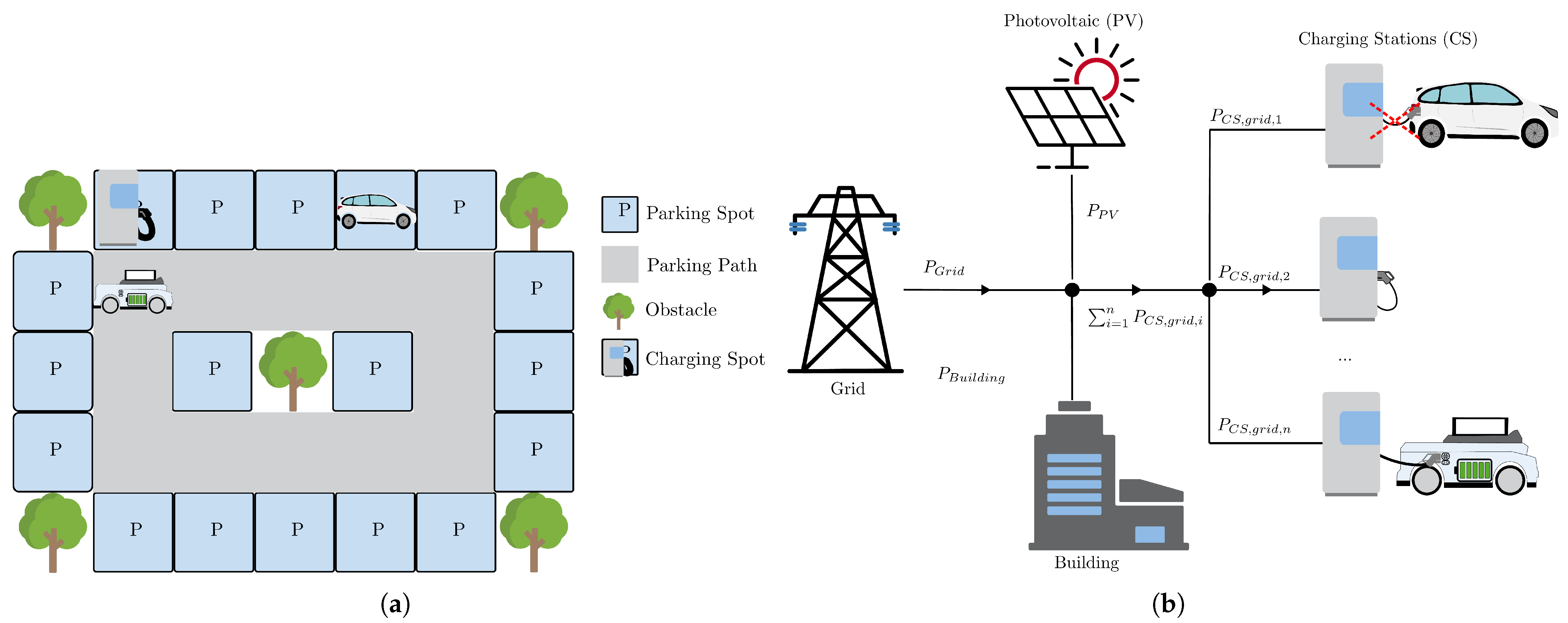
• Charging station index $c\in [1,N_{\mathrm{CS}}]$, referring to a specific charging station or charger location.
• Parking field index $f\in [1,N_{\mathrm{PF}}]$, indicating the designated parking field under consideration.
• Binary variables: All binary variables are indicated by use of the symbol $\delta$. ${\delta }_{\mathrm{mtc},r,c}$ indicates the MCR r is located at CS c. The abbreviation “mtc” is used to denote “move to charger”. ${\delta }_{\mathrm{mtp},r,f}$ indicates the MCR r is located at parking field f. The abbreviation “mtp” is used to denote “move to parking field”.
• Sign convention for continuous variables: The continuous variables describing power satisfy $P_x\in {\mathbb{R}}_{\ge 0}$.

The OP formulation is implemented using Pyomo v.6.9.2 [20]. Pyomo is an open source software package for formulating and solving large-scale optimization problems.

The optimization objective is defined through a cost function that may incorporate terminal costs, state-dependent penalties, control efforts, and costs associated with continuous control variables. In this specific application, the primary goal is to maximize profit. Consequently, the revenue generated by charging EVs using MCRs is taken into account, as described in Equation (1), where the fixed selling price $p_{\mathrm{sell}}$ is multiplied by the total energy delivered by the MCRs. Conversely, the energy procurement cost is based on the time-varying electricity price $p_{\mathrm{buy},k_p}$ and the amount of energy obtained from the grid, as shown in Equation (2). It is assumed that the price profile across the optimization horizon is known in advance. Since the formulation requires a minimization problem, the profit—being the difference between revenue and cost—is represented by multiplying the net cost term by $-1$ (see Equation (3)).

$$\begin{array}{cc}\hfill & f_{revenue}=(\sum _{k_p}(p_{\mathrm{sell}}·\sum _r{P}_{\mathrm{MCR},\mathrm{dchrg},r,k_p}·\Delta t)\hfill \end{array}$$

(1)

$$\begin{array}{cc}\hfill & f_{cost}=\sum _{k_p}{p}_{\mathrm{buy},k_p}·P_{grid,draw,k_p}·\Delta t\hfill \end{array}$$

(2)

$$\begin{array}{cc}\hfill & f_{MPC}=-(f_{revenue}-f_{cost})\hfill \end{array}$$

(3)

The cost function is subject to a set of constraints and the system’s dynamic behavior, which will be detailed in the subsequent sections. All constraints presented are enforced at each time step within the prediction horizon, i.e., for every $k_p\in [0,N_{\mathrm{Horizon}}]$. For readability, the time index $k_p$ will be omitted in the notation unless its inclusion enhances clarity.

As a first constraint, the system must satisfy the power balance at the grid connection point. At each time step $t_{k_p}$, this balance is enforced as defined in Equation (4). To properly account for the direction of energy flow in the cost formulation, it is necessary to distinguish between the power drawn from the grid $P_{\mathrm{grid},\mathrm{draw}}$ and the power fed into the grid $P_{\mathrm{grid},\mathrm{feed}}$. For this purpose, a binary variable ${\delta }_{\mathrm{grid}}$ and corresponding auxiliary equations are introduced, as shown in Equations (5)–(7).

$$\begin{array}{cc}\hfill & P_{\mathrm{grid}}=P_{Building}+\sum _r{P}_{\mathrm{MCR},\mathrm{chrg},r}-P_{\mathrm{PV}}\hfill \end{array}$$

(4)

$$\begin{array}{cc}\hfill & P_{\mathrm{grid}}=P_{\mathrm{grid},\mathrm{draw}}-P_{\mathrm{grid},\mathrm{feed}}\hfill \end{array}$$

(5)

$$\begin{array}{cc}\hfill & P_{\mathrm{grid},\mathrm{draw}}\le M_{\mathrm{big},\mathrm{grid}}·{\delta }_{\mathrm{grid}}\hfill \end{array}$$

(6)

$$\begin{array}{cc}\hfill & P_{\mathrm{grid},\mathrm{feed}}\le M_{\mathrm{big},\mathrm{grid}}·(1-{\delta }_{\mathrm{grid}})\hfill \end{array}$$

(7)

Simultaneous charging from and feeding power back to the grid is not permitted. A direct modeling of this behavior using the binary variable ${\delta }_{\mathrm{grid}}$ in Equation (5) would, however, introduce nonlinearity into the system. To preserve linearity, the big-M formulation is adopted, as proposed in [21]. By incorporating Equations (6) and (7) with a sufficiently large constant $M_{\mathrm{big},\mathrm{grid}}$ (set here to $M_{\mathrm{big},\mathrm{grid}}=1000\mathrm{kW}$), it is guaranteed that only one of the two auxiliary variables representing grid power flow is active at any time step. This approach ensures that the model remains a mixed-integer linear program.

Each MCR must be located at exactly one field, which can either be a parking spot or a charging spot, as stated in Equation (8). Furthermore, each field can only be occupied by a single robot at any given time, as enforced by the constraints in Equations (9) and (10).

$$\begin{array}{cc}\hfill & \sum _c{\delta }_{\mathrm{mtc},r,c}+\sum _f{\delta }_{\mathrm{mtp},r,f}=1\forall r\hfill \end{array}$$

(8)

$$\begin{array}{cc}\hfill & \sum _r{\delta }_{\mathrm{mtc},r,c}\le 1\forall c\hfill \end{array}$$

(9)

$$\begin{array}{cc}\hfill & \sum _r{\delta }_{\mathrm{mtp},r,f}\le 1\forall f\hfill \end{array}$$

(10)

The power capabilities of both the MCRs and the EVs are also bounded and subject to their respective location. Accordingly, the following constraints apply for each MCR r:

$$\begin{array}{cc}\hfill & P_{\mathrm{MCR},\mathrm{chrg},r}\le \sum _c{\delta }_{\mathrm{mtc},r,c}·P_{\max ,\mathrm{charger}}\hfill \end{array}$$

(11)

$$\begin{array}{cc}\hfill & P_{\mathrm{MCR},\mathrm{chrg},r}\le P_{\mathrm{MCR},\mathrm{chrg},\max ,r}\hfill \end{array}$$

(12)

$$\begin{array}{cc}\hfill & P_{\mathrm{MCR},\mathrm{dchrg},r}\le (1-\sum _c{\delta }_{\mathrm{mtc},r,c})·P_{\mathrm{MCR},\mathrm{dchrg},\max ,r}\hfill \end{array}$$

(13)

If an MCR is connected to a charger, its charging power is constrained by the charger’s maximum capability, as defined in Equation (11). Additionally, the MCR’s own maximum charging capability $P_{\mathrm{MCR},\mathrm{chrg},\max ,r}$ imposes a further limit, as given in Equation (12). When not connected to a charger, the discharging power of the MCR, denoted by $P_{\mathrm{MCR},\mathrm{dchrg},r}$, must not exceed its maximum discharging power $P_{\mathrm{MCR},\mathrm{dchrg},\max ,r}$ (see Equation (13)).

Discharging by an MCR is only meaningful if it is co-located with an EV on a parking field. This relationship is modeled using Equations (14) and (15). Specifically, Equation (14) allows the total discharging power to be distributed across all parking locations, while Equation (15) ensures that discharging occurs exclusively at the location where both the MCR and an EV are present.

$$\begin{array}{cc}\hfill & P_{\mathrm{MCR},\mathrm{dchrg},r}=\sum _f{P}_{\mathrm{MCR},\mathrm{dchrg},\mathrm{aux},r,f},\forall r\hfill \end{array}$$

(14)

$$\begin{array}{cc}\hfill & P_{\mathrm{MCR},\mathrm{dchrg},\mathrm{aux},r,f}={\delta }_{\mathrm{mtp},r,f}·P_{\mathrm{EV},f}\hfill \end{array}$$

(15)

Since Equation (15) introduces a nonlinear relationship, it is relaxed using the Big-M technique. This yields a set of linear constraints, given in Equations (16)–(18), which approximate the original condition while preserving the problem’s linear structure.

$$\begin{array}{cc}\hfill & P_{\mathrm{MCR},\mathrm{dchrg},\mathrm{aux},r,f}\le M_{\mathrm{dchrg}}·{\delta }_{\mathrm{mtp},r,f},\forall r,f\hfill \end{array}$$

(16)

$$\begin{array}{cc}\hfill & P_{\mathrm{MCR},\mathrm{dchrg},\mathrm{aux},r,f}\le P_{\mathrm{EV},f},\forall r,f\hfill \end{array}$$

(17)

$$\begin{array}{cc}\hfill & P_{\mathrm{MCR},\mathrm{dchrg},\mathrm{aux},r,f}\ge P_{\mathrm{EV},f}-M_{\mathrm{dchrg}}(1-{\delta }_{\mathrm{mtp},r,f}),\forall r,f\hfill \end{array}$$

(18)

Power delivery to an EV is only permitted if an EV is currently present or is expected to arrive at a given prediction step $k_p$. This condition is enforced through Equation (19).

$$\begin{array}{cc}\hfill & P_{\mathrm{EV},k,f}\le {\delta }_{EV,avail,f}\sum _r({\delta }_{\mathrm{MCR},\mathrm{field},r,f}·P_{\mathrm{MCR},\mathrm{dchrg},\max ,r})\forall f\hfill \end{array}$$

(19)

$$\begin{array}{cc}\hfill & P_{\mathrm{EV},f}\ge 0\hfill \end{array}$$

(20)

The change in the energy state $E_{\mathrm{MCR},k,r}$ of the MCRs is determined by the difference between the charging power $P_{\mathrm{MCR},\mathrm{chrg},k,r}$ and the discharging power $P_{\mathrm{MCR},\mathrm{dchrg},k,r}$, integrated over time, and added to the previous energy state $E_{\mathrm{MCR},k-1,r}$, as described in Equation (22).

For the EVs, a similar approach is applied, but only the charging power $P_{\mathrm{EV},f}$ is considered. The energy requirement $\Delta E_{\mathrm{EV},\mathrm{req},k_p,f}$ represents the difference in energy needed at field f to reach the desired state of charge.

$$\begin{array}{cc}\hfill & E_{\mathrm{MCR},k_p=0,r}=E_{\mathrm{MCR},\mathrm{obs},r}\hfill \end{array}$$

(21)

$$\begin{array}{cc}\hfill & E_{\mathrm{MCR},k_p>0,r}=E_{\mathrm{MCR},k_p-1,r}+(P_{\mathrm{MCR},\mathrm{chrg},k_p,r}-P_{\mathrm{MCR},\mathrm{dchrg},k_p,r})·\Delta t\hfill \end{array}$$

(22)

$$\begin{array}{cc}\hfill & \Delta E_{\mathrm{EV},\mathrm{req},k_p=0,f}=\Delta E_{\mathrm{EV},\mathrm{obs},f}\hfill \end{array}$$

(23)

$$\begin{array}{cc}\hfill & \Delta E_{\mathrm{EV},\mathrm{req},k_p>0,f}=\Delta E_{\mathrm{EV},k_p-1,f}-P_{\mathrm{EV},k_p,f}·\Delta t\hfill \end{array}$$

(24)

As part of the receding horizon optimization approach, at each time step $t_k$, an observation o is received from the environment. This observation serves as the basis for updating the optimization problem formulation. As indicated in Equation (23), the energy request $\Delta E_{\mathrm{EV},\mathrm{req},k_p,f}$ for an EV at the current time step k (i.e., $k_p=0$) depends on this state. Additionally, the availability of EVs ${\delta }_{\mathrm{EV},\mathrm{avail},k,f}$ must also be updated. While the requested energy $\Delta E_{\mathrm{EV},\mathrm{obs},f}$ can be directly obtained from the environment, the availability for the current time step ${\delta }_{\mathrm{EV},\mathrm{avail},k_p=0,f}$ is known. The future availability—and therefore the duration of stay—is estimated based on the average historical stay duration. It is important to note that, in this initial version of the MPC controller, no explicit forecasting is applied. Only the EVs currently present in the parking area are considered in the optimization problem, and no assumptions are made regarding the arrival of new EVs within the prediction horizon.

2.2. Limitations of the Initial Approach

The proposed MPC will be tested over a representative two-day period, from 00:00 on 2nd June 2023 to 24:00 on 3rd June 2023. The results will be analyzed, and strategies for improving and extending the MPC will be derived.

For solving the OP, the Gurobi solver [22] is used. It should be noted that, particularly when dealing with multiple MCRs and longer prediction horizons, solving the problem exactly using the default solver settings is not feasible due to the large problem size and complexity. Consequently, less stringent settings have been applied, as summarized in Appendix A.

The resulting trajectory from applying the MPC controller outlined in Section 2.1 to the simulation environment is shown in Figure 2. A prediction horizon of 96 steps, each lasting 5 min, was applied.

In the top graph (a), the power balance, including contributions from the charging stations (CSs), the building, and the PV array, is shown. Over the two-day period, 26 recharging events are identified by the spikes in $P_{\mathrm{CS}}$, which also affect the grid power $P_{\mathrm{Grid}}$. In the bottom graph (e), the number of EVs present in the parking area is depicted. It can be observed that a maximum of five EVs are present at any given time, with the highest occupancy occurring between 12:00 h and 18:00 h on both days. Notably, EV arrivals are sparse during the nighttime hours. In graph (c), the state of charge (SoC) of the MCR is shown. Upon the arrival of the first EVs, the MCR discharges down to 20% SoC. Subsequently, the SoC fluctuates between 10% and 50%, reflecting the brief charging and discharging periods. Even during the night, when no EVs arrive for several hours, the SoC remains around 40%. The cost structure, based on accumulated revenue from energy sold $c_{\mathrm{energy},\mathrm{sold}}$ and electricity costs $c_{\mathrm{energy},\mathrm{bought}}$, is displayed in plot (b). It is observed that during the first day, $c_{\mathrm{energy},\mathrm{sold}}$ temporarily exceeds $c_{\mathrm{energy},\mathrm{bought}}$; however, after 19:00 h, as EVs are no longer present and building power $P_{\mathrm{Building}}$ persists through the night, $c_{\mathrm{energy},\mathrm{bought}}$ remains above $c_{\mathrm{energy},\mathrm{sold}}$. The increase in $c_{\mathrm{energy},\mathrm{sold}}$ is significantly higher on the first day compared to the second day, primarily due to the starting SoC of 100% and higher, more stable PV power. By the end of the second day, the difference between $c_{\mathrm{energy},\mathrm{sold}}$ and $c_{\mathrm{energy},\mathrm{bought}}$ results in a profit of EUR −15.29.

Several aspects of the strategy implemented by the MPC controller are unsatisfactory. The following key observations should be highlighted:

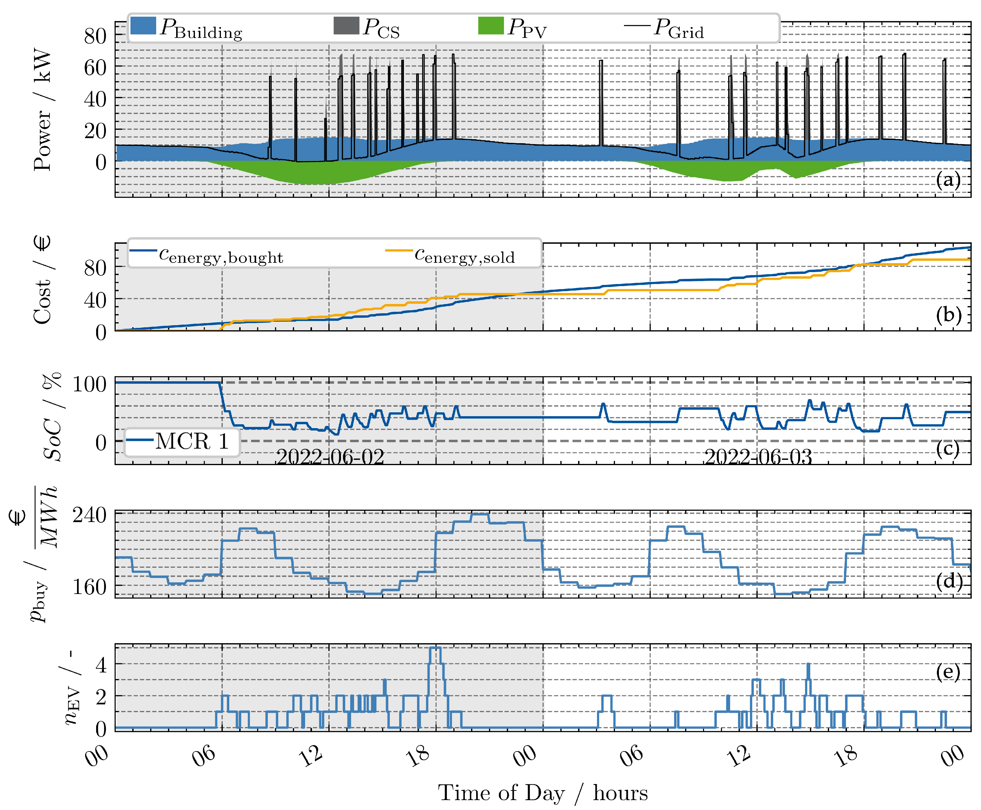
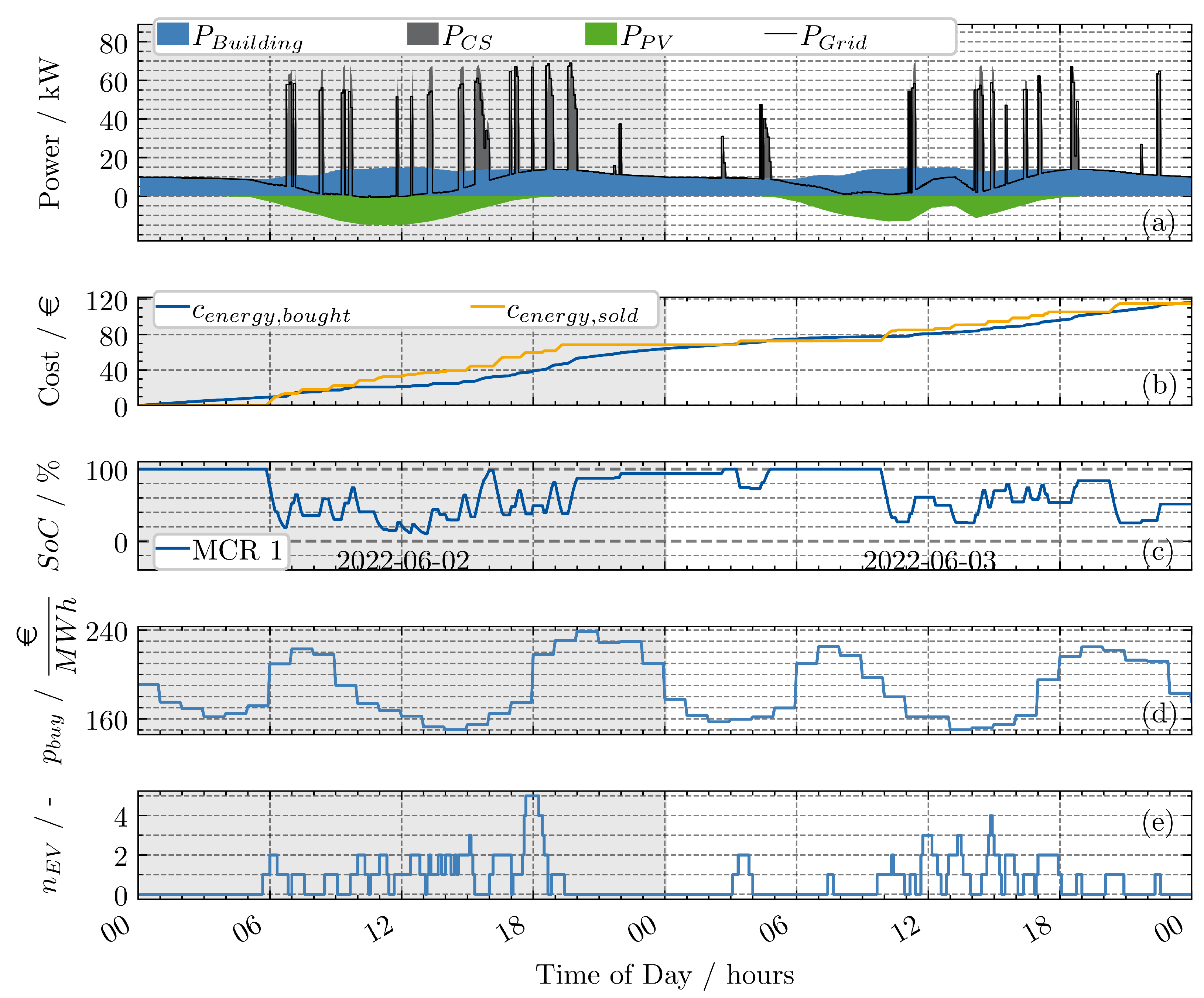
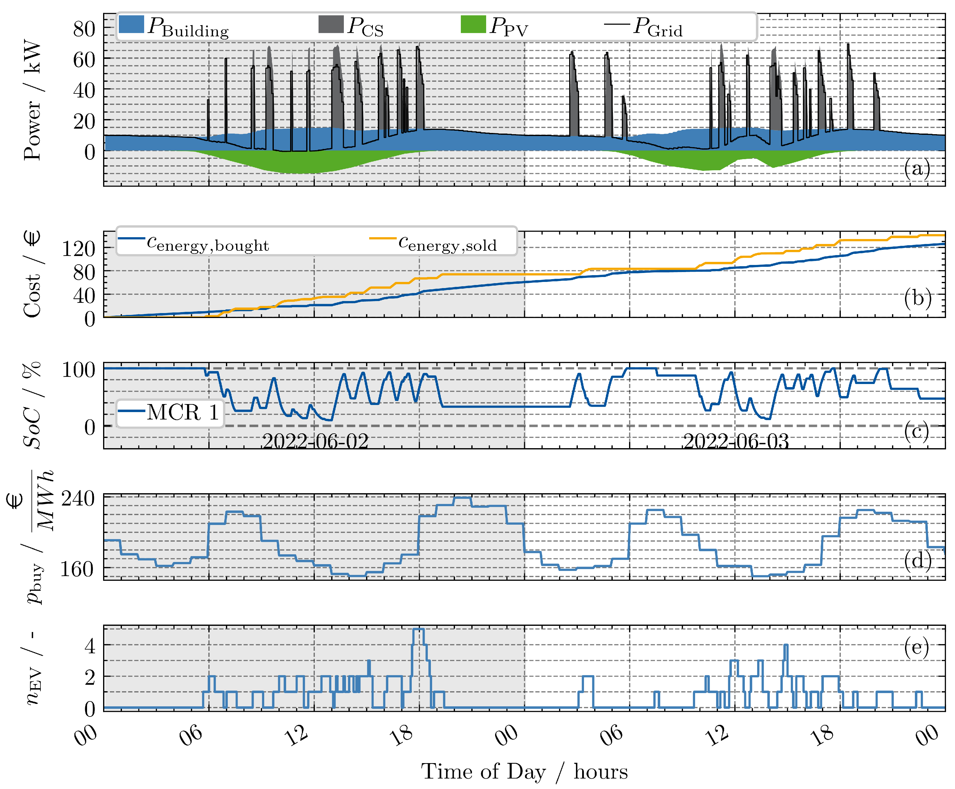
• No recharging without EVs being present: In general, the MCR only recharges if EVs are present, which is strategically not a good time, because the EVs might already be gone until the MCR is recharged. Especially during the period between 20:00 h and 04:00 h, there are no EVs at the parking area. Therefore, the MCR could be recharged. Due to the structure of the optimization problem, where recharging is only a viable option if an EV is present to which the charged energy could be sold, this does not happen.
• No “smart” charging: It is observed that, in most cases, the MCR operates at a high power level of approximately 50 kW. However, the charging times do not correspond to periods of low energy costs (refer to plot (d)) or periods of high PV power. It is hypothesized that if charging times and power were to be synchronized with electricity prices and PV power, costs could be reduced.

In summary, the observations suggest that the MPC controller is limited in its ability to anticipate future revenue, primarily due to its inability to account for the potential revenue from EVs not currently present at the parking area.

To address these shortcomings, two alternative approaches are proposed. The first approach introduces a penalty for not recharging during idle periods, incentivizing more consistent operation. The second approach incorporates a forecasting model to predict future EV arrivals, utilizing long short-term memory (LSTM) networks. The training process and integration of this forecasting model into the MPC controller are described in detail.

2.3. Penalty for Not Recharging

One of the main drawbacks identified in the basic MPC approach is its inability to recharge during extended periods of inactivity. To address this, the OP formulation is extended to encourage the controller to initiate recharging, ideally during times when no EVs are present at the parking area.

The solution implementation requires the following specifications:

• Mobile Charging Robots (MCRs) should recharge even if there are no EVs present at the parking area currently or within the prediction horizon. Thus, not recharging should incur higher (virtual) costs compared to recharging.
• The charging of an EV should still take priority over the MCR recharging itself.

In light of the specified requirements, a penalty term (Equations (25) and (26)) is introduced, which extends the cost function outlined in Equation (3).

$$\begin{array}{cc}\hfill & f_{\mathrm{Penalty}}=p_{\mathrm{penalty},\mathrm{slack}}·{ϵ}_{\mathrm{slack},\mathrm{MCR},\mathrm{SoC}}\hfill \end{array}$$

(25)

$$\begin{array}{cc}\hfill & f_{\mathrm{MPC},\mathrm{pen}}=f_{\mathrm{MPC}}+f_{\mathrm{Penalty}}\hfill \end{array}$$

(26)

The penalty term $f_{\mathrm{Penalty}}$ is added to the original cost function $f_{\mathrm{MPC}}$. It is computed based on the slack variable ${ϵ}_{\mathrm{slack},\mathrm{MCR},\mathrm{SoC}}$ and a penalty parameter $p_{\mathrm{penalty},\mathrm{slack},\mathrm{k}}$. The slack variable ${ϵ}_{\mathrm{slack},\mathrm{MCR},\mathrm{SoC}}$ is incorporated into Equation (27).

$$\begin{array}{c}\hfill E_{\mathrm{MCR},k_p=N_{\mathrm{Horizon}},r}\ge E_{\mathrm{MCR},\mathrm{total}}-{ϵ}_{\mathrm{slack},\mathrm{MCR},\mathrm{SoC}}\end{array}$$

(27)

The slack variable ${ϵ}_{\mathrm{slack},\mathrm{MCR},\mathrm{SoC}}$ represents the difference between the total energy of the MCR battery $E_{\mathrm{MCR},\mathrm{total}}$ and the actual energy of the MCR at the end of the prediction horizon $E_{\mathrm{MCR},k_p=N_{\mathrm{Horizon}},r}$. This variable, in conjunction with the cost function, penalizes not reaching a 100% SoC by the end of the horizon. It is important to carefully consider the value of $p_{\mathrm{penalty},\mathrm{slack}}$. If the penalty for deviation from 100% SoC is set too high, the MCR would prioritize charging even when EVs are available that could be charged. Conversely, if the penalty is set too low, the cost of purchasing energy from the grid would remain the dominant factor. Therefore, the parameter is defined dynamically based on the current electricity price $p_{\mathrm{buy},k_p}$ and the selling price $p_{\mathrm{sell}}$, as shown in Equations (28)–(30).

$$\begin{array}{cc}\hfill p_{\mathrm{buy},\max ,\mathrm{horizon}}& =\underset{k_p\in [0,N_{\mathrm{Horizon}}]}{max}{p}_{\mathrm{buy},k_p}\hfill \end{array}$$

(28)

$$\begin{array}{cc}\hfill {\overline{p}}_{\mathrm{penalty},\mathrm{slack}}& =p_{\mathrm{buy},\max ,\mathrm{horizon}}+{\epsilon }_{\mathrm{buy},\max }\hfill \end{array}$$

(29)

$$\begin{array}{cc}\hfill p_{\mathrm{penalty},\mathrm{slack}}& =\left\{\begin{array}{cc}{p}_{\mathrm{sell}}·0.8,\hfill & \mathrm{if}{\overline{p}}_{\mathrm{penalty},\mathrm{slack}}\ge p_{\mathrm{sell}}\hfill \\ {\overline{p}}_{\mathrm{penalty},\mathrm{slack}},\hfill & \mathrm{otherwise}\hfill \end{array}\right.\hfill \end{array}$$

(30)

First, it is ensured that the penalty is greater than the maximum price over the horizon, $p_{\mathrm{buy},\max ,\mathrm{horizon}}$, as shown in Equations (28) and (29). Here, ${\epsilon }_{\mathrm{buy},\max }$ can be chosen as a very small value relative to $p_{\mathrm{buy},\max ,\mathrm{horizon}}$, for example, EUR 0.01. Next, Equation (30) ensures that the penalty does not exceed the potential revenue from charging EVs. Thus, it is set below the selling price in case the preliminary calculated penalty cost ${\overline{p}}_{\mathrm{penalty},\mathrm{slack}}$ is greater $p_{\mathrm{sell}}$.

The terminal penalty method implicitly assumes that if no EV is present, recharging the MCR is the best possible strategy. While this is typically the case in practice, this method does not account for smart charging with (forecasted) knowledge of future EV arrivals. Therefore, the following section introduces a second approach that incorporates forecasting.

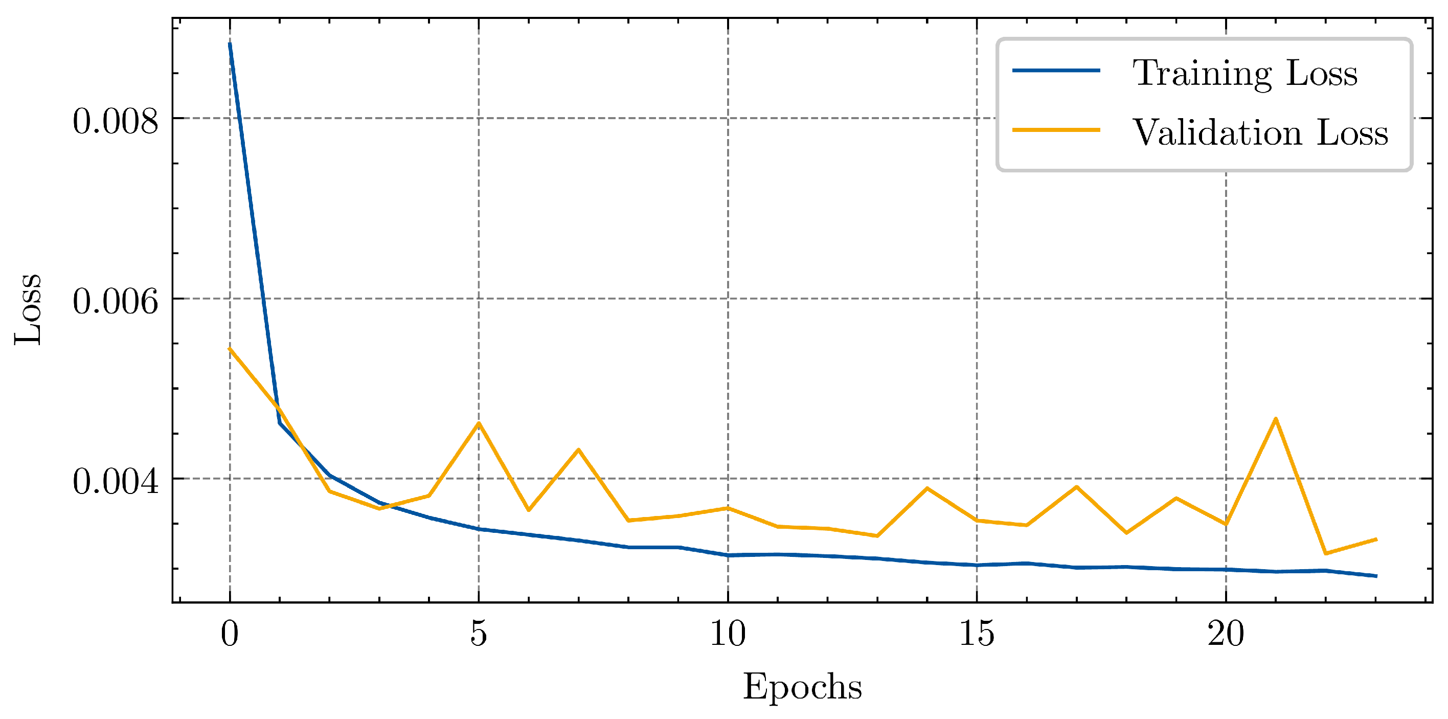
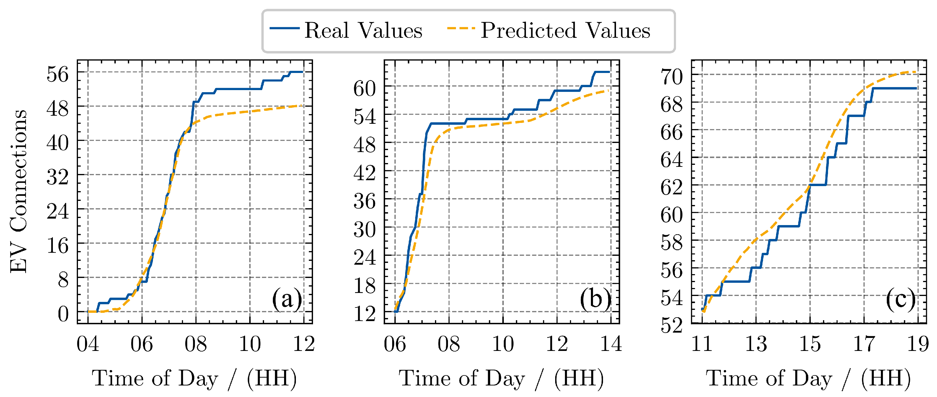
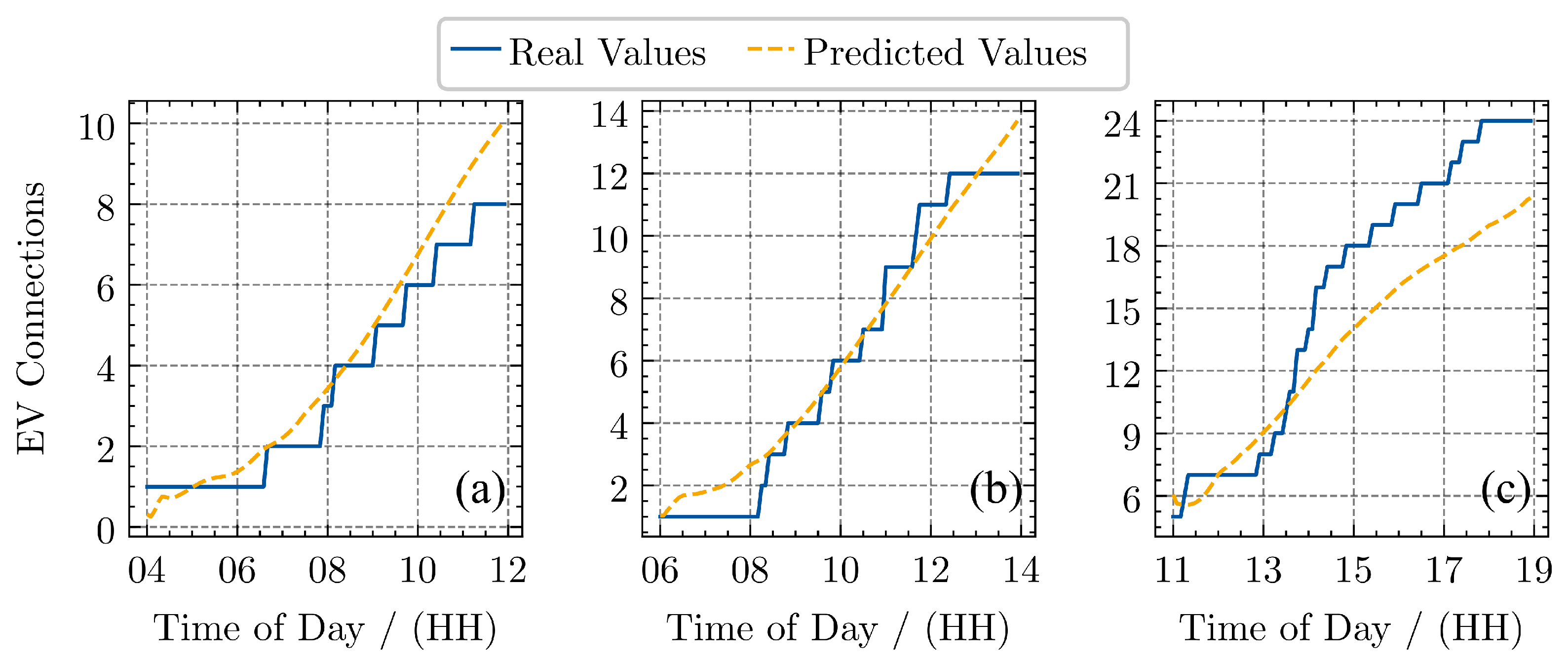
2.4. LSTM Forecasting for MPC

The following section outlines the methodology for forecasting EV arrivals over a prediction horizon. Long short-term memory (LSTM) networks are commonly used for forecasting EV behavior, and they are well suited for this application since they can continuously update predictions based on the observed input. A significant challenge in this context is the lack of real-world data from charge points with actual MCRs. The available dataset from a supermarket parking area is limited and does not fully align with the simulated use case. To address this, a two-step approach is applied. First, an LSTM model is trained using a large dataset from a different use case (an office building with numerous charging stations) to demonstrate the general applicability of the approach. Then, an artificial dataset is generated from the available supermarket dataset to further train the model.

The LSTM forecasting model is designed to make predictions for a large time period based on a single input step. In this case, the prediction horizon of the MPC is set to 8 h, corresponding to 96 steps, with a time step size of 5 min. At each input step, five pre-processed features are provided, derived from three raw values. The date-related data are encoded using sin/cos encoding to maintain continuity and avoid artificial “jumps”. In sin/cos encoding, for instance, days of the week (ranging from zero to six, representing Monday to Sunday) are mapped to a sine and cosine period. An overview of the input features and outputs is provided in

Table 3. Input (x) and output ($\widehat{y}$) from LSTM.

Variable	Raw Value	Processing	Processed Variable
$x_{ToD}$	Time of Day (ToD)	Sin/Cos Encoding:	${\overline{x}}_{\mathrm{ToD},\sin }$, ${\overline{x}}_{\mathrm{ToD},\cos }$
$x_{DoW}$	Day of Week (DoW)	Sin/Cos Encoding	${\overline{x}}_{\mathrm{DoW},\sin }$, ${\overline{x}}_{\mathrm{DoW},\cos }$
$x_{\mathrm{accum}}$	Accumulated arrived EVs	normalized accumulated arrived EVs	${\overline{x}}_{\mathrm{accum}}$
${\widehat{y}}_{\mathrm{accum}}$	Accumulated arrived EVs	normalized accumulated arrived EVs	${\widehat{y}}_{\mathrm{accum}}\in [0,N_{\mathrm{Horizon}}]$

.

In Figure 3, the results from training with the ACN dataset [23] are displayed. Although the training loss decreases more significantly and steadily compared to the validation loss, improvements can be observed in both sets.

The prediction performance on the test set is illustrated in Figure 4, where results for three different days and three different starting times are shown.

In graph (a), the prediction is conducted at 04:00 h on 24 February 2020. The input consists of the sin/cos encoded day of the week and time of day. Additionally, the input for the accumulated EVs $x_{\mathrm{accum}}$ is zero, as no EVs have connected to the charging stations up to that point. At around 05:00 h, EVs begin to arrive, and between 06:00 h and 08:00 h, there is a sharp increase in the number of connected EVs. The forecast tracks this increase very precisely; however, the final value of 56 EVs at 12:00 h is slightly underestimated (48 EVs predicted). For the second date, between 06:00 h and 14:00 h, the prediction quality improves further, though a slight underestimation persists. For the third day, where the prediction is made at 11:00 h for the following 8 h, the forecast slightly overestimates the number of connected EVs.

Overall, the performance of the model appears satisfactory for the examined cases. However, performance could likely improve by adding more input features, such as a label for holidays or the time of year. As this work focuses on investigating potential improvements to the base MPC controller, the approach is now applied to the supermarket parking area with an MCR.

For the transfer of the approach, a synthetic dataset is created. To achieve this, the distribution of arrivals from a real-world charging location dataset is considered, and a standard deviation is applied to this distribution. Subsequently, the distribution is scaled, and data are sampled for a whole year from this distribution.

Exemplary results on a test dataset, which is not part of the training data, are shown in Figure 5. In graph (c), for the third prediction interval, the value at the end of the prediction horizon is slightly underestimated (24 real and 20 in forecast). However, in general, the forecasting performance appears to be satisfactory.

Note that the applied approach should only serve as a reference to investigate how the base MPC controller can be improved. For a comprehensive forecasting approach, at least two shortcomings have to be investigated further:

• Dataset: Within the synthetic dataset, there is an assumption regarding how the data are distributed, which might not account for the actual distribution observed in a real dataset. This would need careful investigation and suitable data, ideally coming from an actual field trial with MCRs.
• Input Features: The input features of the LSTM are selected as a minimum set. For comprehensive forecasting, more input features would need to be applied. For example, it can be assumed that during holidays, fewer people charge at supermarkets.

In this part, the MPC controller was introduced with a focus on the formulation of the OP. The limitations of the base approach were analyzed. Subsequently, two approaches to improve the base MPC controller were presented. The first approach introduces a terminal penalty to incentivize recharging of the MCR even if no EVs are present. The second approach incorporates a forecasting model based on LSTM networks to predict future EV arrivals. The next section will present the results from applying these two approaches to the simulation environment and compare them with the base MPC controller and an MPC controller with perfect forecast.

3. Results

In the last section, an MPC with an underlying MILP was introduced. The limitations of applying the raw MPC controller were discussed, and two approaches to improve the controller were presented. Consequently, in this section, the results from applying the different approaches are compared. In order to understand the limitations of the two approaches, especially looking at the sensitivity to unprecise forecasts, a run with a perfect forecast is presented as well. In this context, a perfect forecast means that the MPC controller has full insights about the arrival and departure time of all EVs within the prediction horizon. Further, the requested energy by these EVs is assumed to be known. Oppositely, with the LSTM forecast model, only the arrival time is forecasted. The stay duration is forecasted as the historical average and corrected if an EV leaves earlier or stays longer. The requested energy is assumed to be known precisely, once an EV arrives. This assumption is considered reasonable, as the European DC charging communication standard [24] specifies that the EV is responsible for communicating its requested energy for the initiated charging session. The section is concluded with a comparative simulation study, including the MPC LSTM approach and the approach with terminal penalty. The analysis comprises multiple runs for different seasons in order to consider the sensitivity with regard to PV share, electricity prices and EV arrival schemes.

3.1. Terminal Penalty

The results from adding this penalty to the OP are depicted in Figure 6.

It can be observed that the desired behavior of recharging during night is achieved, which also leads to a less negative profit. Due to $p_{\mathrm{penalty},\mathrm{slack}}$, which enforces recharging, no smart charging behavior can be observed. For example, if the MCR had recharged after 02:00 h instead of already fully recharging at 20:00 h on the previous day, the price and hence the overall cost would have been reduced. Nevertheless, results indicate that for the given problem, the approach with using a terminal penalty can be a viable option, especially in cases where the focus is one availability rather than smart charging capabilities.

3.2. Perfect Forecast as Reference

In order to obtain an understanding of how a strategy with full foresight would operate, another simulation run is performed, where the MPC controller is provided with a perfect forecast. The run with a perfect forecast is shown in Figure 7. It can be observed that the MPC controller now charges extensively during the night, right before the first EVs arrive at 4:00 h and the electricity price is very low. Similarly, this can be observed on the first day before the price rises at 18:00 h and on the second day at 14:00 h, where the price is low.

The final revenue with the perfect forecast is significantly higher compared to the base strategy (EUR 140.70 compared to RU 88.27), and a positive net profit of EUR 14.64 is received.

3.3. LSTM Forecasting

In Figure 8, the base MPC controller was extended with the LSTM forecasting and applied to the simulation environment.

The same configuration as in the previous runs was selected. The major difference compared to the perfect forecast reference is that at the first day after 18:00 h, it is not discharged as much as seen with the perfect forecast; moreover, the SoC stays at 100% SoC during night. This is due to a misprediction of an EV arriving late. Nevertheless, the performance is significantly improved compared to the base approach and also shows higher profit compared to the penalty strategy (EUR 7.85 vs. EUR −1.15).

It can be concluded that both presented approaches improve upon the base approach. The LSTM-based approach offers more potential for charging during times with a low cost or high PV penetration, but relies on the forecast quality.

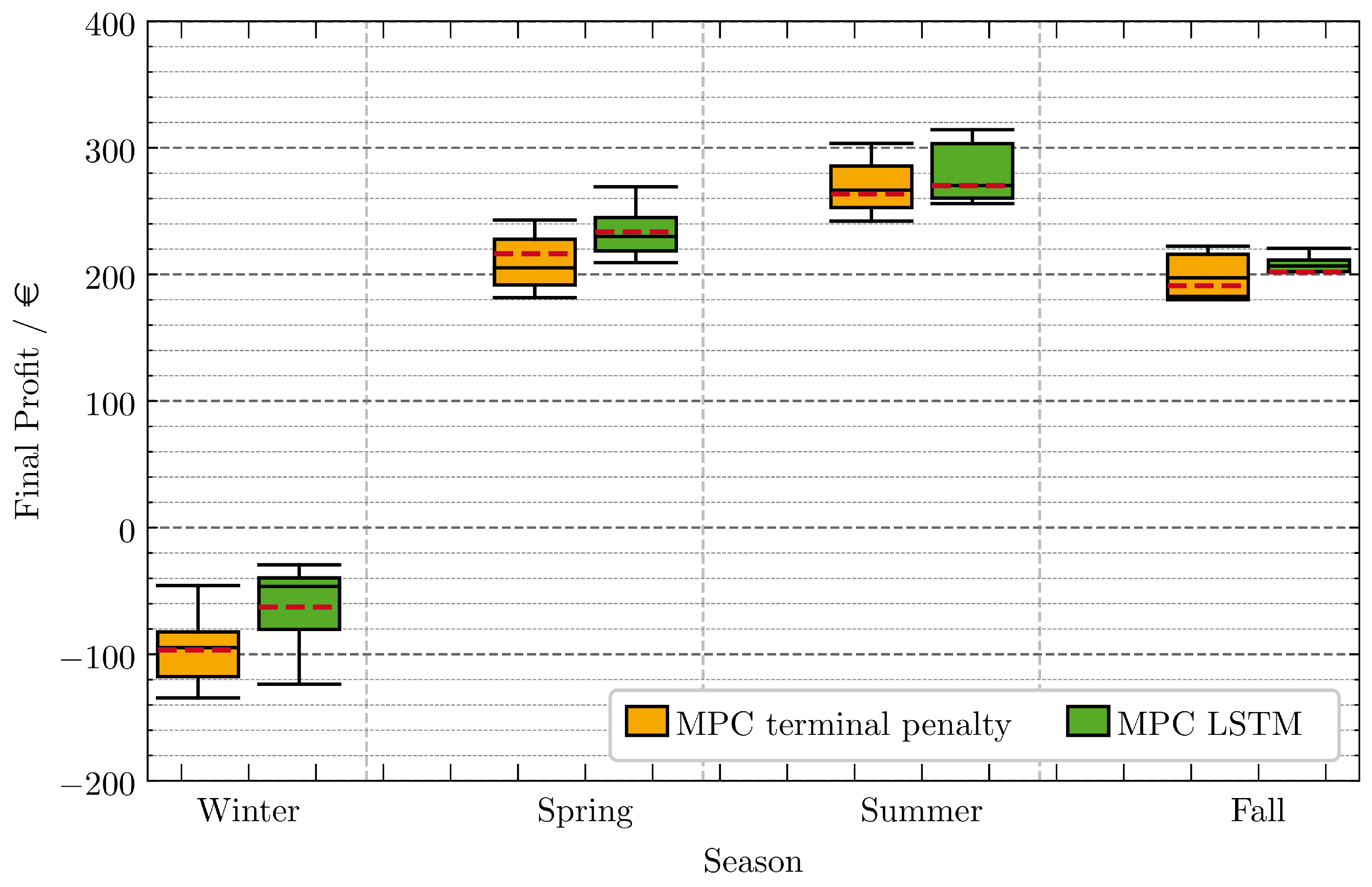
3.4. Comparative Analysis Study

In the following sections, a comparative analysis of the MPC LSTM and the MPC approach with a terminal penalty will be provided in terms of their performance in achieving the objective of an operating strategy that maximizes profit. To perform the comparative simulation study, the configuration in

Table 4. Environment configuration for analysis.

Parameter	Description	Value
$N_{\mathrm{CS}}$	Number of CSs on parking area	1
$P_{\mathrm{CS},\max }$	Maximum charging power of the CSs	50 kW
$E_{\mathrm{building},\mathrm{yearly}}$	Yearly consumption of supermarket building	200,000 $\mathrm{kWh}$
$P_{\mathrm{PV},\mathrm{peak}}$	Peak power of installed PV array	40 $\mathrm{kW}$
$n_{\mathrm{avg},\mathrm{EV},\mathrm{hourly}}$	Average arriving EVs per hour	1
$N_{\mathrm{MCR}}$	Number of MCR in the environment	2

is utilized.

As defined in the configuration, two MCRs will be present in the environment, but only one CS will be recharged. On average, one EV will arrive per hour. Most EVs will arrive between noon and early evening. The annual building consumption and PV peak power are configured to be within typical ranges, with the potential to provide a slight PV surplus under ideal conditions.

Four scenarios are selected, each spanning a duration of one week. For each scenario, multiple runs are performed with EV arrivals sampled from a probability distribution provided by the simulation environment. As these scenarios represent a week in the respective season of the year, they are named accordingly as follows:

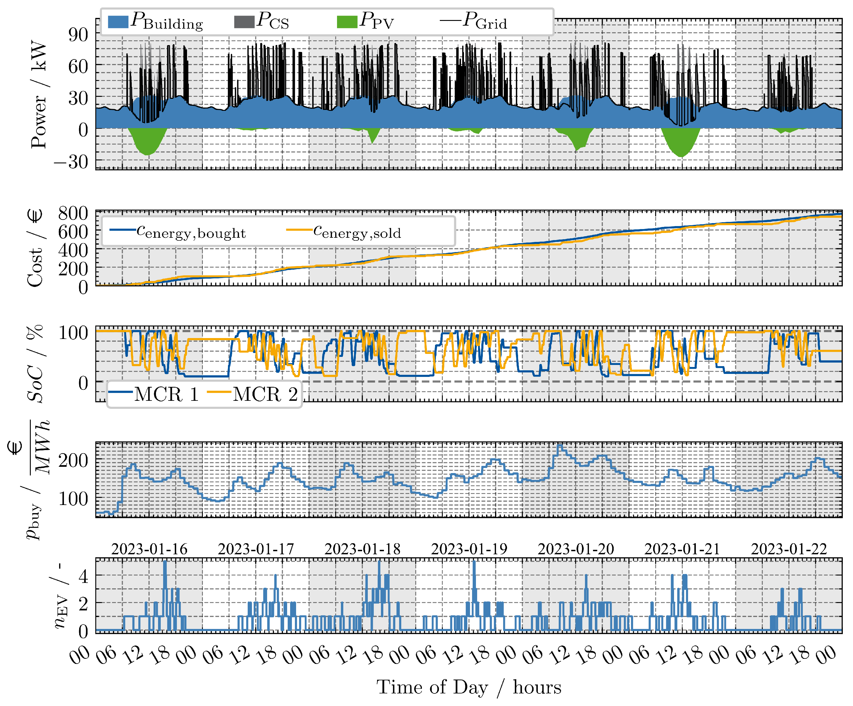
• Winter: 19 January 2023 00:00 h to 25 January 2023 24:00 h (7 runs).
• Spring: 3 April 2023 00:00 h to 9 April 2023 24:00 h (7 runs).
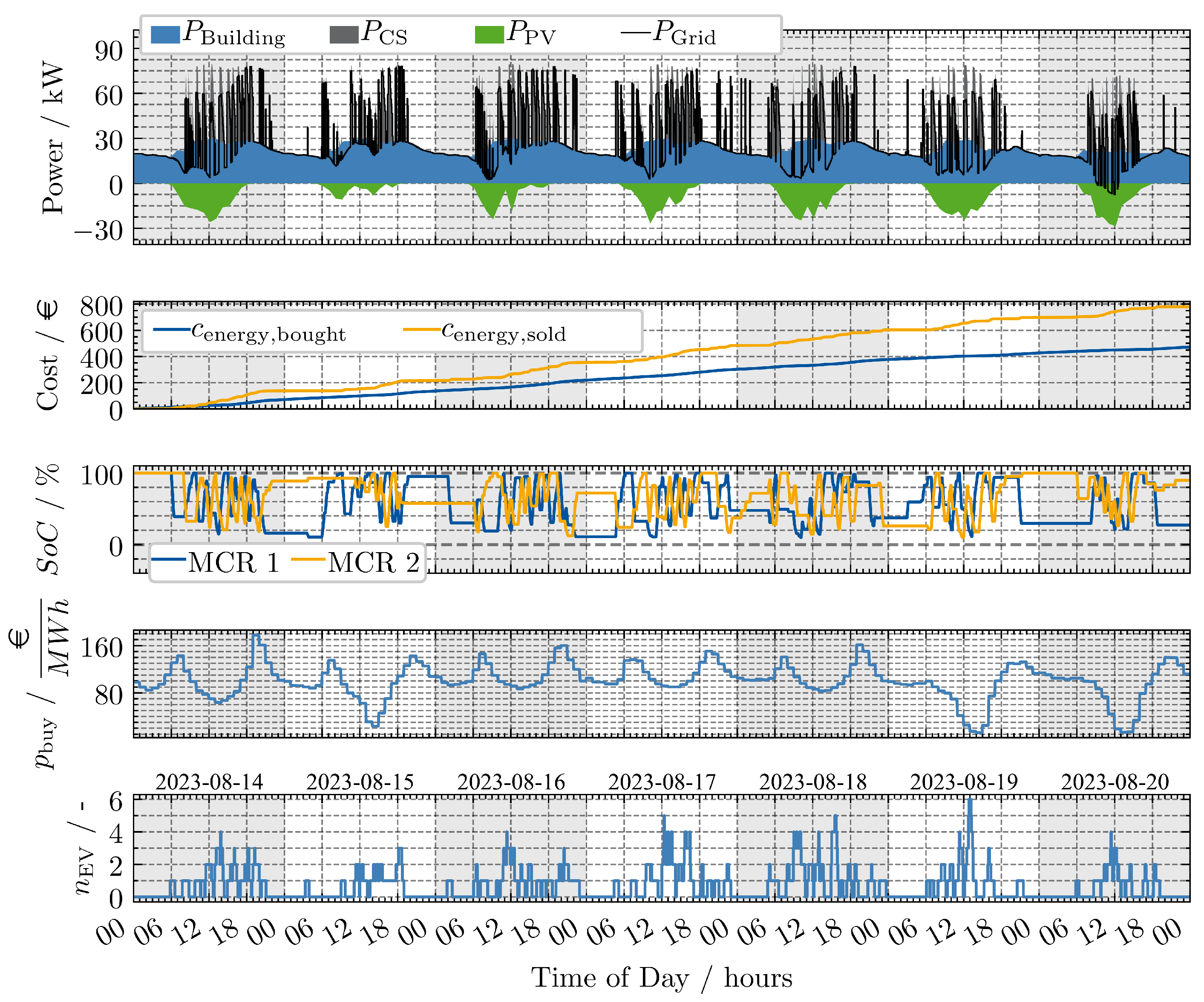
• Summer: 14 August 2023 00:00 h to 20 August 2023 24:00 h (7 runs).
• Fall: 16 October 2023 00:00 h to 22 October 2023 24:00 h (6 runs).

For the MPC approach with a terminal penalty, the horizon is kept at 10 steps with a 5 min step width, as presented in the previous section. The prediction horizon for the MPC LSTM approach is reduced to 24 steps in order to avoid overly long computation times, as these scale already due to the longer simulated time period duration (one week vs. 2 days) and the increased number of MCRs (two vs. one).

In Figure 9, the profit for the two approaches for every scenario is depicted. The figure shows the statistics of the performed runs as box plots. In contrast to classic box plots, the mean value is added in a dashed red line in addition to the median. The boundaries of the box represent the upper and lower quantiles, meaning that 25% of the data are greater/lower than this value. The whiskers represent the least and greatest values excluding outliers. To be concise in the analysis, comparative statements will refer to the mean value if not further specified. The traces of a single run with the MPC LSTM approach are shown in Appendix B to obtain an understanding of the variance in the electricity price and EV arrival schemes. Generally, it can be observed that the winter scenario shows the lowest profits, with values around EUR 0 (hence losses). Conversely, the summer scenario shows the highest mean profits. This is in accordance with the expectation that higher PV power due to more sunny hours in the summer leads to a lower energy cost compared to the winter. Additionally, the summer scenario shows lower and more fluctuating energy prices (see Appendix B).

By comparing the two approaches, it can be observed that the mean profit is highest for the MPC LSTM throughout all seasons. However, especially for the summer and fall scenarios, the difference between the summer and the fall scenario is not significant. In the fall scenario, the best run with a terminal penalty shows an even higher profit than the MPC LSTM approaches’ corresponding run.

This study confirms the comparison performed in the previous section based on a single scenario: The MPC LSTM performs, on average, better compared to the approach with an added terminal penalty. However, for the given study, the difference appears not to be very significant, which could be attributed to the reliance on forecast quality and the shorter prediction horizon necessary to allow for reasonable computation times. Further, the supermarket setting involves a lot of charging demand during mid-day, lowering the chances for smart recharging with PV power.

4. Discussion

The presented methodology allows extending MPC-based charging management to the utilization of MCRs. In contrast to charging management with stationary charging infrastructure, not only the CSs are considered; the model considers all parking spot fields. Hence, the model allows us not only to control the charging power but also to control the movement of the MCRs in an optimized fashion. For a computationally feasible model, the nonlinearities are linearized and the big-M method is used. As a suitable strategy requires some assumptions about the future, especially the arrival of EVs, two approaches were proposed.

The first approach relies on a terminal penalty. It performs better than the base approach, but has still some limitations. These become apparent when comparing the results with the perfect forecast. It can be seen that with the perfect forecast, major recharging of the MCR is performed at times when the electricity price is low (first day at 14:00 h; second day at 03:00 h and 14:00 h). This is not the case with the terminal penalty. The recharging here is performed as soon as the MCR is not needed for charging EVs, but not necessarily at the times when the electricity price is low.

The approach with the LSTM forecast shows a further improvement compared to the terminal penalty approach; however, due to the mispredictions, the performance is still not as good as the perfect forecast. At the lowest electricity prices during noon of the first and second days, the MCR is recharged; however, with the LSTM approach, recharging is carried out in the evening of the first day instead of during the night, at the time when the price is lowest. This highlights that the LSTM approach is still sensitive to mispredictions, especially in regard to the EVs arriving in the evening.

As the exact number of EVs and the time of arrival of the last EV of the corresponding day is impossible to forecast precisely, this limitation is difficult to overcome. However, it might be feasible to optimize this over a number of scenarios. For example, when having adequate statistics of the likelihood of more EVs arriving after a current time (e.g., 19:00), the MPC could optimize over the scenarios with weighted probabilities. This would increase the complexity of the problem but could lead to a more robust solution. Additionally, allowing for bidirectional charging of the MCRs could improve the performance. In case of a misprediction in the evening, the MCR could still feed back the energy later at a high price level and recharge at a low price.

According to the findings of the literature, the LSTM prediction model in our study was applied to a charging management problem that includes MCRs for the first time. Other charging management problems, where LSTMs have usually been applied, target more regular distributions as they focus, for example, on office parking areas [16]. Further, the sensitivity to the forecast of the last EV of the day is mainly due to the inclusion of MCRs, which has not yet investigated in the literature. Therefore, it is recommended that the prediction accuracy and the impact of prediction accuracy on MPC performance is further investigated for the presented problem.

The comparative analysis performed in Section 3.4 confirms the improved performance of MPC LSTM compared to the approach with a terminal penalty but suggests that there are some limitations remaining as the differences are not as significant as could be expected.

The presented MPC framework effectively integrates forecasting with real-time updates; however, certain limitations remain, which are summarized here. The accuracy of energy request and stay duration predictions is constrained by the reliance on historical averages. Additionally, the MILP formulation requires simplifications to maintain computational efficiency, leading to the omission of SoC-dependent efficiencies and power limits. The exclusion of field distances may result in suboptimal MCR positioning in large parking areas. Furthermore, the AI-based forecast model was validated using a dataset that differs from the actual MCR use case, necessitating further validation with more representative data. The profit results are subject to the assumptions made in regard to the buying and selling prices of energy. For the selling price, a typical price for the German market for the corresponding power range was chosen (EUR 0.5). Considering the EV user as not price-sensitive, the profit would of course be higher with a higher assumed selling price. Therefore, the selling price is deemed suitable for comparative purposes, but price sensitivity of EV users and even dynamic selling prices are not considered. For the buying price, the German electricity trade fair price from 2023 is considered. With the rapidly increasing share of renewables in Germany (as well as in many other countries), the price structure throughout the day changes as well. While there were 301 h with negative prices in 2023, there were already 459 h in 2024. At the same time, the average price fluctuation during one day increased from 98 €$/\mathrm{MWh}$ to 118 €$/\mathrm{MWh}$ (derived from [25]). Both makes flexibility options more attractive and promotes higher profits for smart charging applications. Therefore, the overall profits presented are highly sensitive in regard to the examined year.

Despite these limitations, the developed methods provide a strong foundation for further advancements, such as extending MCR functionalities for grid support and refining prediction models with more tailored datasets.

The methodology of MPC charging management presented in this work focuses on MRCs. However, the methodology can be applied to analogous fields in which the recharging process must be synchronized with the movement of rechargeable (robotic) devices. In recent years, Unmanned Aerial Vehicles (UAVs), also known as drones, have been the focus of extensive research for various applications, including the inspection of power grids, pipelines, and renewable power plants [26]. For these applications, sophisticated in-flight charging algorithms have been proposed by [26,27]. In the future, research should be conducted based on integrating these in-flight charging algorithms into a high-level charging management system by applying the presented approach.

References

1. Europeans Are Generally Positive Towards e-Mobility. 2024. Available online: https://transport.ec.europa.eu/news-events/news/europeans-are-generally-positive-towards-e-mobility-2024-06-20_en (accessed on 17 July 2025).
2. International Energy Agency. Global EV Outlook 2024. 2024. Available online: https://www.iea.org/reports/global-ev-outlook-2024 (accessed on 23 July 2025).
3. Wessel, P.; Faßbender, M.; Gerz, J.; Andert, J. Designing a Prototype of a Mobile Charging Robot for Charging of Electric Vehicles; SAE Technical Paper Series; SAE International400 Commonwealth Drive: Warrendale, PA, USA, 2024. [Google Scholar] [CrossRef]
4. Faßbender, M.; Rößler, N.; Eisenbarth, M.; Andert, J. An Electric Vehicle Charging Simulation to Investigate the Potential of Intelligent Charging Strategies. Energies 2025, 18, 2778. [Google Scholar] [CrossRef]
5. Towers, M.; Kwiatkowski, A.; Terry, J.; Balis, J.U.; de Cola, G.; Deleu, T.; Goulão, M.; Kallinteris, A.; Krimmel, M.; KG, A.; et al. Gymnasium: A Standard Interface for Reinforcement Learning Environments. arXiv 2024, arXiv:2407.17032. [Google Scholar]
6. Huang, Q.; Yang, L.; Jia, Q.S.; Qi, Y.; Zhou, C.; Guan, X. A Simulation-Based Primal-Dual Approach for Constrained V2G Scheduling in a Microgrid of Building. IEEE Trans. Autom. Sci. Eng. 2023, 20, 1851–1863. [Google Scholar] [CrossRef]
7. Huang, Q.; Yang, L.; Hou, C.; Zeng, Z.; Qi, Y. Event-Based EV Charging Scheduling in a Microgrid of Buildings. IEEE Trans. Transp. Electrif. 2023, 9, 1784–1796. [Google Scholar] [CrossRef]
8. Huang, Q.; Jia, Q.S.; Guan, X. A Multi-Timescale and Bilevel Coordination Approach for Matching Uncertain Wind Supply With EV Charging Demand. IEEE Trans. Autom. Sci. Eng. 2017, 14, 694–704. [Google Scholar] [CrossRef]
9. Fallah-Mehrjardi, O.; Yaghmaee, M.H.; Leon-Garcia, A. Charge Scheduling of Electric Vehicles in Smart Parking-Lot Under Future Demands Uncertainty. IEEE Trans. Smart Grid 2020, 11, 4949–4959. [Google Scholar] [CrossRef]
10. Yang, W.; Fang, H.; Xu, D.; Jiang, B.; Shi, P. A Stochastic Model Predictive Control Based Energy Management Approach for Microgrids with Electric Vehicles. IEEE Trans. Transp. Electrif. 2024, 11, 3137–3145. [Google Scholar] [CrossRef]
11. Nguyen, H.T.; Choi, D.H. Distributionally Robust Model Predictive Control for Smart Electric Vehicle Charging Station with V2G/V2V Capability. IEEE Trans. Smart Grid 2023, 14, 4621–4633. [Google Scholar] [CrossRef]
12. Ju, Y.; Zeng, T.; Allybokus, Z.; Moura, S. Robo-Chargers: Optimal Operation and Planning of a Robotic Charging System to Alleviate Overstay. IEEE Trans. Smart Grid 2024, 15, 770–782. [Google Scholar] [CrossRef]
13. Yang, L.; Geng, X.; Guan, X.; Tong, L. EV Charging Scheduling Under Demand Charge: A Block Model Predictive Control Approach. IEEE Trans. Autom. Sci. Eng. 2024, 21, 2125–2138. [Google Scholar] [CrossRef]
14. Yang, Y.; Yeh, H.G.; Nguyen, R. A Robust Model Predictive Control-Based Scheduling Approach for Electric Vehicle Charging With Photovoltaic Systems. IEEE Syst. J. 2023, 17, 111–121. [Google Scholar] [CrossRef]
15. D’Amore, G.; Cabrera-Tobar, A.; Petrone, G.; Pavan, A.M.; Spagnuolo, G. Integrating model predictive control and deep learning for the management of an EV charging station. Math. Comput. Simul. 2024, 224, 33–48. [Google Scholar] [CrossRef]
16. McClone, G.; Ghosh, A.; Khurram, A.; Washom, B.; Kleissl, J. Hybrid Machine Learning Forecasting for Online MPC of Work Place Electric Vehicle Charging. IEEE Trans. Smart Grid 2024, 15, 1891–1901. [Google Scholar] [CrossRef]
17. Hermans, B.; Walker, S.; Ludlage, J.; Özkan, L. Model predictive control of vehicle charging stations in grid-connected microgrids: An implementation study. Appl. Energy 2024, 368, 123210. [Google Scholar] [CrossRef]
18. Dante, A.W.; Kelouwani, S.; Agbossou, K.; Henao, N.; Bouchard, J.; Hosseini, S.S. A Stochastic Approach to Designing Plug-In Electric Vehicle Charging Controller for Residential Applications. IEEE Access 2022, 10, 52876–52889. [Google Scholar] [CrossRef]
19. Li, W.; Zhang, T.; Wang, R. Energy Management Model of Charging Station Micro-Grid Considering Random Arrival of Electric Vehicles. In Proceedings of the 2018 IEEE International Conference on Energy Internet (ICEI), Beijing, China, 21–25 May 2018; pp. 29–34. [Google Scholar] [CrossRef]
20. Bynum, M.L.; Hackebeil, G.A.; Hart, W.E.; Laird, C.D.; Nicholson, B.L.; Siirola, J.D.; Watson, J.P.; Woodruff, D.L. Pyomo—Optimization Modeling in Python; Springer International Publishing: Cham, Switzerland, 2021; Volume 67. [Google Scholar] [CrossRef]
21. Bertsimas, D.; Tsitsiklis, J.N. Introduction to Linear Optimization; Athena Scientific Books; Dynamic Ideas and Athena Scientific: Belmont, MA, USA, 1997; Volume 7. [Google Scholar]
22. Gurobi Optimization, LLC. Gurobi Optimizer Reference Manual; 2023. Available online: https://www.gurobi.com (accessed on 23 July 2025).
23. Lee, Z.J.; Li, T.; Low, S.H. ACN-Data: Analysis and Applications of an Open EV Charging Dataset. In Proceedings of the Tenth International Conference on Future Energy Systems (e-Energy ’19), Phoenix, AZ, USA, 25–28 June 2019. [Google Scholar] [CrossRef]
24. ISO 15118-2:2014; Road Vehicles—Vehicle to Grid Communication Interface—Part 2: Network and Application Protocol Requirements. International Organization for Standardization: Geneva, Switzerland, 2014. Available online: https://www.iso.org/standard/55366.html (accessed on 23 July 2025).
25. Burger, B. Spot Market Prices|Energy-Charts. 2025. Available online: https://www.energy-charts.info/charts/price_spot_market/chart.htm?l=de&c=DE (accessed on 17 July 2025).
26. Gu, Y.; Wang, J.; Liang, Z.; Zhang, Z. Flexible Constant-Power Range Extension of Self-Oscillating System for Wireless In-Flight Charging of Drones. IEEE Trans. Power Electron. 2024, 39, 15342–15355. [Google Scholar] [CrossRef]
27. Gu, Y.; Wang, J.; Liang, Z.; Zhang, Z. Mutual-Inductance-Dynamic-Predicted Constant Current Control of LCC-P Compensation Network for Drone Wireless In-Flight Charging. IEEE Trans. Ind. Electron. 2022, 69, 12710–12719. [Google Scholar] [CrossRef]
Figure 1. Overview of simulation environment: (a) Parking area where MCRs and EVs are located. (b) Power balance within the simulation environment.
Energies 18 03948 g001
Figure 2. MPC controller without forecast model and horizon of 96 steps (8 h): (a) power contributions at charge point; (b) accumulated cost and revenue; (c) SoC of MCR; (d) electricity price; (e) number of EVs at charge point. Final profit: EUR −15.29 (cost: EUR 103.56; revenue: EUR 88.27).
Energies 18 03948 g002
Figure 3. Training loss LSTM.
Energies 18 03948 g003
Figure 4. Exemplary prediction with test set for ACN dataset with 8 h of prediction horizon: (a) Mo 24 February 2020 4:00 h–12:00 h; (b) Mo 3 February 2020 06:00 h–14:00 h; (c) Tu 21 January 2020 11:00 h–19:00 h.
Energies 18 03948 g004
Figure 5. Exemplary prediction with test set for synthetic supermarket dataset with 8 h of prediction horizon: (a) Fr 1 December 2023 4:00 h–12:00 h; (b) Mo 7 December 2023 06:00 h–14:00 h; (c) Sa 12 December 2023 11:00 h–19:00 h.
Energies 18 03948 g005
Figure 6. Without explicit prediction, terminal cost—horizon 10 steps (50 min): (a) power contributions at charge point; (b) accumulated cost and revenue; (c) SoC of MCR; (d) electricity price; (e) number of EVs at charge point. Final profit: EUR −1.15 (cost: EUR 116.26; revenue: EUR 115.11 ).
Energies 18 03948 g006
Figure 7. MPC with perfect forecast and horizon of 96 steps (8 h): (a) power contributions at charge point; (b) accumulated cost and revenue; (c) SoC of MCR; (d) electricity price; (e) number of EVs at charge point. Final profit: EUR 14.64 (cost: EUR 126.06; revenue: EUR 140.70).
Energies 18 03948 g007
Figure 8. LSTM prediction with horizon of 96 steps (8 h): (a) power contributions at charge point; (b) accumulated cost and revenue; (c) SoC of MCR; (d) electricity price; (e) number of EVs at charge point. Final profit: EUR 7.85 (cost: EUR 124.71; revenue: EUR 132.56).
Energies 18 03948 g008
Figure 9. Profit comparison for MPC LSTM and MPC terminal penalty approach for different scenarios.
Energies 18 03948 g009